Modelling Pluvial Flooding in Urban Areas Coupling the Models Iber and SWMM


Department of Civil Engineering, Water and Environmental Engineering Group, Universidade da Coruña, Elviña, 15071 A Coruña, Spain
*
Author to whom correspondence should be addressed.
Water 2020, 12(9), 2647; https://doi.org/10.3390/w12092647
Submission received: 31 July 2020
/
Revised: 17 September 2020
/
Accepted: 18 September 2020
/
Published: 22 September 2020
(This article belongs to the Special Issue Modelling of Floods in Urban Areas)
Abstract
:Dual urban drainage models allow users to simulate pluvial urban flooding by analysing the interaction between the sewer network (minor drainage system) and the overland flow (major drainage system). This work presents a free distribution dual drainage model linking the models Iber and Storm Water Management Model (SWMM), which are a 2D overland flow model and a 1D sewer network model, respectively. The linking methodology consists in a step by step calling process from Iber to a Dynamic-link Library (DLL) that contains the functions in which the SWMM code is split. The work involves the validation of the model in a simplified urban street, in a full-scale urban drainage physical model and in a real urban settlement. The three study cases have been carefully chosen to show and validate the main capabilities of the model. Therefore, the model is developed as a tool that considers the main hydrological and hydraulic processes during a rainfall event in an urban basin, allowing the user to plan, evaluate and design new or existing urban drainage systems in a realistic way.
1. Introduction
The rise of impervious areas in cities due to urbanization has increased the occurrence of flooding and its consequences during extreme rainfall events. In order to mitigate flood impacts it is essential for cities to have a drainage network properly planned and designed. Urban drainage systems are made of two clearly different subsystems: the sewer (minor) network and the surface (major) network. During a rainfall event, the water exchange between both subsystems can be in both directions through inlets and manholes. The surface overland flow, the sewer flow and the exchange between both of them are commonly computed using dual drainage models that solve all the processes in an integrated and realistic way [1,2,3,4].
The first dual drainage approaches were 1D/1D models that simplify the surface flow as open channels or ponds, solving the 1D Saint-Venant equations [5]. Modelling a street as an open channel is a sensible approach as long as the water velocities presents a preferent direction [6]. However, the flow in urban districts has a significant two-dimensional behaviour that is necessary to consider in the numerical modelling in order to achieve truthful results. Therefore, 1D/2D dual drainage models were developed, that solve the two-dimensional shallow water equations on the surface while maintaining the one-dimensional approach in the sewer network [7,8,9]. These 1D/2D approaches, combined with accurate digital elevation models (DEM), allow modellers to obtain more realistic results. There are different 1D/2D dual drainage models, some of them developed on research works [10], others with licensed software such as Infoworks ICM or Mike-Urban. To date, there are some free distribution 1D/2D drainage models that solve surface and sewer flow and their interaction but there are not usually used in real projects of engineering with guarantee and user-friendliness.
Storm Water Management Model (SWMM) [11] model is used frequently as 1D sewer network engine in 1D/2D urban drainage models. Thus, coupling SWMM with overland flows models solves the limitation of SWMM to simulate and visualise the flood area. There exist multiple methods of coupling SWMM with overland flows models [9,12,13,14,15,16,17,18,19,20,21] in which different coupling methodologies are used. Some models modify or adapt the SWMM code [12] while others call SWMM libraries and functions without editing the engine code [9]. Regarding the flow exchange, there are models that considerer only a unidirectional exchange from sewer network to the surface [13,15] and others that consider a bidirectional exchange that allows flow enter to the sewer [14]. The election of the overland flow model determines the complexity of the dual model and its computation time. In this way, for overland flow, there is a wide variety of models based on the equations of fully dynamic shallow water and others based on simplified models as the local inertial model, diffusive wave model or the kinematic wave [16].
In addition, there is commercial software such as XP-SWMM [20], PCSWMM [22], Mike-Urban [21] or FLO-2D Pro that couple SWMM engine with 2D overland flow models.
In this work, a 1D/2D dual urban drainage model is developed linking two free distributed hydraulic models: Iber [23] and SWMM [11]. The model links the Iber source code with the SWMM Dynamic-link Library (DLL), which contains functions that allow simulation data to be exchanged between SWMM and other software. The SWMM dynamics libraries used here were developed in [24], and up to now, they have not been implemented in any 1D/2D dual drainage model. The model presented here is therefore a new free tool that allows an accurate and complete analysis of the flood area extension and its duration due to the bidirectional exchange implemented. The validation of the model is shown in three different test cases that demonstrate its capabilities.
2. Materials and Methods
2.1. Hydraulic Models
2.1.1. Iber
Iber is a 2D numerical model for simulating turbulent free surface flow and transport processes in shallow waters [23,25]. It is a free distribution software that can be downloaded at www.iberaula.com. The hydrodynamics module of Iber solves the 2D depth-averaged shallow water equations, also known as dynamic wave equations to distinguish them from simpler diffusive and kinematic wave models. The model also incorporates several hydrological processes, and its application to rainfall-runoff and overland flow computations has been validated in previous works [26,27,28,29]. The mass and momentum conservation equations solved by the model can be written as follows:
where is the water depth, , and are the two components of the unit discharge and its modulus, is the bed elevation, is the Manning coefficient, is the gravity acceleration, is the rainfall intensity, and is the infiltration rate.
The hydrodynamic equations are solved with an unstructured finite volume solver, including a specific numerical scheme for hydrological applications, the so-called DHD scheme [26]. The use of this scheme is strongly recommended in rainfall-runoff computations.
2.1.2. SWMM 5.1
The Storm Water Management Model (SWMM) is a 1D dynamic sewer network model developed for the simulation of rainfall-runoff processes and the conveyance of water flows through drainage systems. The sewer network is modelled as a network of links (pipes) connected by nodes (manholes). The hydrodynamics module of SWMM solves the 1D Saint-Venant equations for gradually varied, unsteady flow. These are referred to as dynamic wave analysis and are implemented in the module EXTRAN (Extended Transport) [30].
2.2. Linking Methodology
The structure of SWMM5 allows its interaction and linking with the source code of Iber. The SWMM5-DLL is built from the source code of the OWA-SWMM Open-Source Library [24]. The OWA-SWMM source code is written in C++ and includes a Toolkit API that allows to get and set all the model parameters and hydraulic variables before, during and after the simulation. Once the SWMM-DLL is built, it can be directly invoked from the source code of Iber, and no further actions are needed. Despite new GPU-parallelized releases of Iber are coded in C++ [27], in this work we have used the standard Iber code, which is written in FORTRAN. Therefore, as the OWA-SWMM is written in C++, a standard intrinsic module has been incorporated at the Iber code to stablish the interoperability between the two languages.
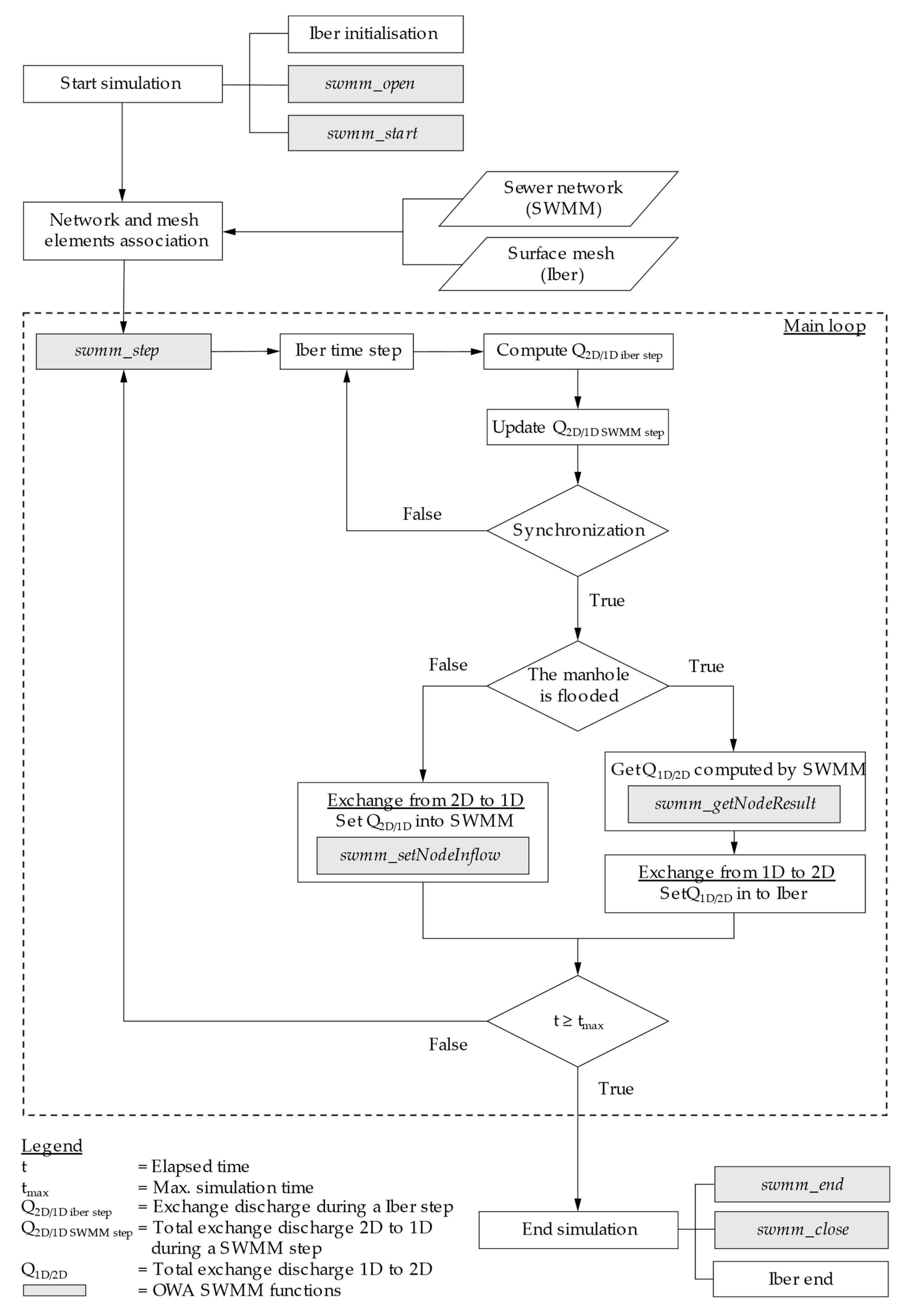
The linking methodology includes a set of subroutines that are added to the Iber source code, in order to invoke the SWMM functions and other related operations. In Figure 1, a flow diagram of the 1D/2D linking methodology is presented. Before starting the simulation, each inlet and manhole defined in SWMM must be associated to a surface mesh element in Iber. This can be done automatically (nearest neighbour) or manually by the user. Each inlet and manhole can be assigned to one or more surface elements. This might be appropriate depending on the spatial scale of the study case and the mesh resolution, as it will be shown in the next section.
In a similar way, before the simulation starts, the roof elements defined in Iber are associated to the nearest manhole in SWMM.
Once the simulation starts, at each time step the model solves the surface and sewer flow equations. The surface and sewer network equations are computed by the two solvers in an independent way, using different time steps. The time step in Iber depends on a Courant–Friedrichs–Lewy (CFL) stability constraint that relates the maximum permissible computational time step, the grid size, the flow velocity and the water depth [26]. Similarly, the time step in SWMM is computed by a Courant condition that limited the time step to the time needed for a wave to propagate through the entire pipe [30]. Therefore, a time step synchronization is necessary to guarantee a correct coupling between models and to do the water exchange between minor and major drainage networks at the same elapsed time. The time step of SWMM is usually larger than the Iber time step; thus, the SWMM elapsed time is considered as the synchronization time. The synchronization implies that, at certain computation steps, the Iber time step must be adjusted in order to avoid to exceed the elapsed time of SWMM [9,31]. In order to do so, the computational time step in Iber is defined as follows:
where is the time step of Iber for the step n + 1, adjusted to the synchronization with SWMM if it was necessary, and are the SWMM and Iber time steps computed independently in both models for the step n + 1 (i.e., without considering synchronization), is the time of the last synchronization, and is the elapsed time of Iber.
The water exchange is done every time at which the models are synchronized, assuming a constant water discharge during the whole time step. The interaction between the overland flow and the sewer drainage system occurs only through inlets and manholes. The surface water can only enter the sewer network through the inlets, while the water can only return to the surface through the manholes. This last assumption is reasonable due to when the system is surcharged, the volume of water returned through the inlets is negligible respect the volume returned through the manholes. However, if a manhole is flooded, all the inlets associated to it will not caught any surface flow.
The inlets are directly connected to manholes. In the present version, the conveyance time between the inlet and the manhole is not considered, i.e., the water that enters an inlet is instantaneously directed to the manhole associated to that inlet. This assumption is reasonable since in real applications the conveyance time between inlets and manholes is usually negligible compared to the conveyance time through the major and minor drainage networks. Furthermore, even if detailed studies about the flow in inlets have been performed in the last years [32,33], information about the conduits that link inlets and manholes is usually not available in real case studies.
Roofs are also directly connected to manholes. Thus, all the rain that falls in a roof element is automatically added to the associate manhole regardless the roof height and its conveyance time. Moreover, the roofs will add flow to the manhole node regardless of whether it is flooded or not. It is highlighted that the conveyance time can be included to the model if the information of the roof is available. In addition, the official version will also include the possibility of modelling SuDS (Sustainable Drainage System) techniques such as green roofs or permeable pavements, among others.
To compute the aforementioned interactions between Iber and SWMM, the exchanged discharge introduced in the sewer network is calculated in Iber. Thus, as Iber has a time step smaller than SWMM, for each of the n Iber time steps that are needed to complete a SWMM time step, the cumulative volume of water exchanged is evaluated. Then, when the synchronization occurs, the functions of SWMM are invoked to introduce the volume caught by the inlets in the sewer between the previous and the current synchronization time as a manhole discharge. Free weir, submerged weir and orifice equations used in previous studies [9,10,31] have been implemented to compute the flow interchange depending on the water level at the surface mesh element, the mesh element elevation and the hydraulic head at the manhole. On the other hand, if a manhole is flooding, the node flood discharge is computed by SWMM and transferred to the surface as an Iber source. It is highlighted that the same water volume that is extracted from Iber is introduced in SWMM and, vice versa. Finally, SWMM step is computed establishing the next synchronization time and it will not run again until Iber reaches this synchronization time and new exchange occurs.
3. Case Studies and Results
In order to validate the dual drainage model presented in Section 2 and to show its capabilities, three case studies have been modelled. The case studies were chosen in order to assess numerical aspects such as mass conservation and numerical stability, to validate model output against laboratory experimental data and to show the workflow methodology to set up a model in a real application. The study cases include free surface and surcharged flow conditions in the drainage network as well as water discharge exchanges in both directions, i.e., from major to minor network and vice versa. All the tests have been solved using the DHD scheme of Iber and a wet-dry threshold of 0.1 mm.
3.1. Simplified Urban Street
3.1.1. Case Study Description
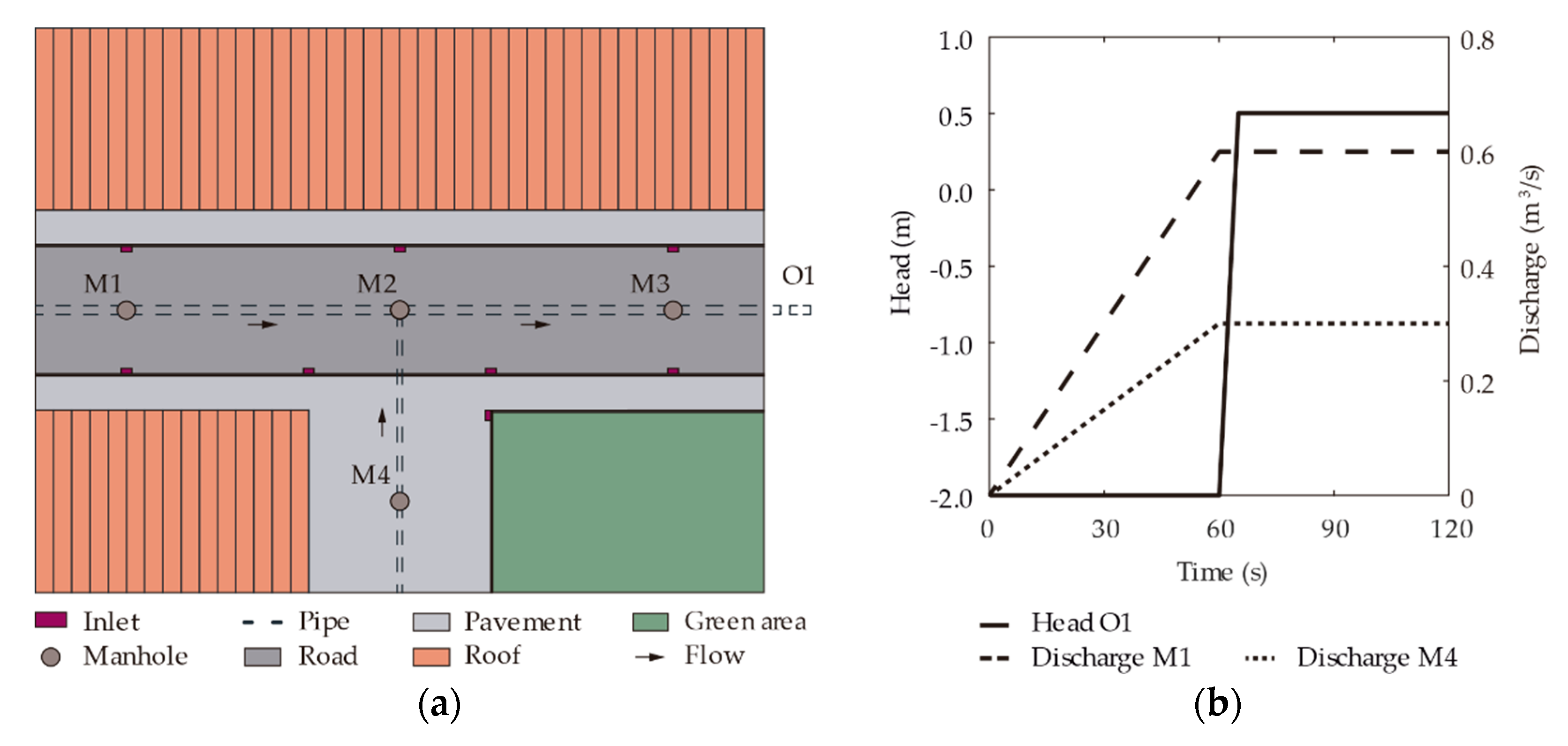
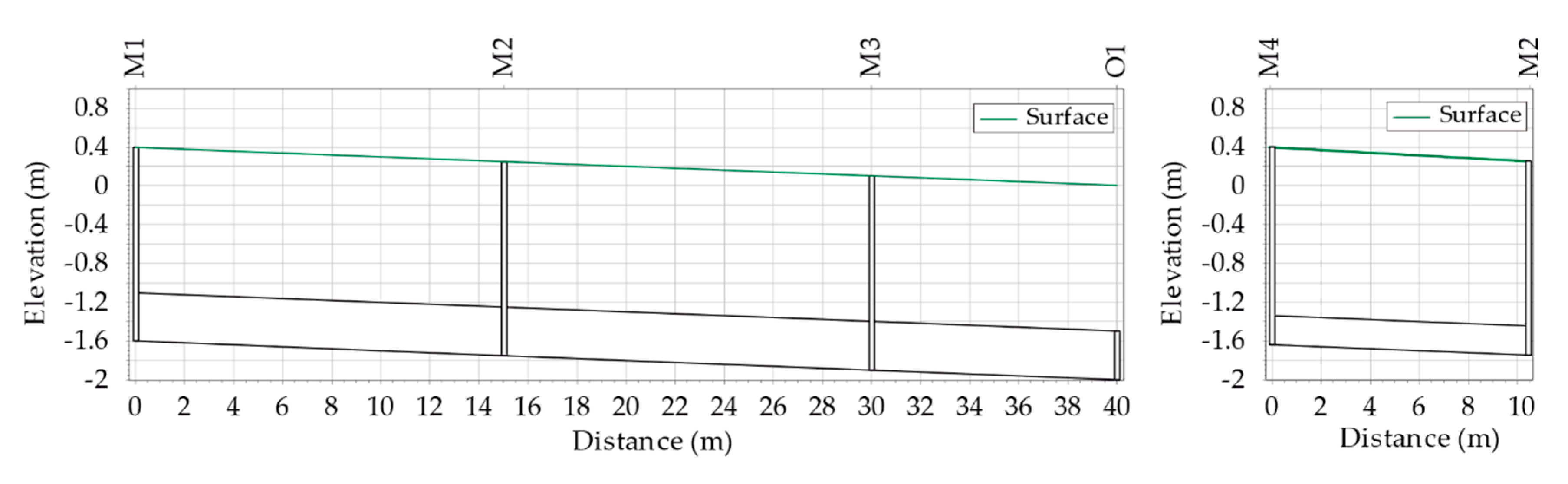
This case study consists in a synthetic urban street, and it is aimed to verify some numerical aspects and basic capabilities of the model. The spatial domain includes a roadway with pavements at both sides, a pedestrian area, a green area and buildings (Figure 2a). The roadway is 40 m in length and 7 m in width, and it is separated from the 2-m wide pavements by a 15-cm high curb. The roadway and pavements have 2% and 1% slopes in the transversal direction, respectively, and 1% longitudinal slope. The buildings are 10 m in width and are directly connected to the manholes. The sewer system and the surface are connected by 8 inlets and 4 manholes. Each inlet is connected to its nearest manhole. Manholes M1, M2 and M3 are connected by a pipe with an inner diameter of 500 mm, while the pipe that connects manholes M4 and M2 has in inner diameter of 300 mm. Both pipes have a slope of 1%. The network outlet (O1) is located 10 m downstream from manhole M3, following the pipe slope, and its invert elevation is −2 m (Figure 3). The invert manhole relative depth regarding the surface is −2 m for M1, M2 and M3 and −2.05 m for M4. At O1, the reference elevation for the head is the surface elevation, 0 m in this location.
In order to simulate surcharged flow and surface flood conditions, two inlet hydrographs were imposed at manholes M1 and M4, and a hydraulic head condition was fixed at the outlet O1, as shown in Figure 2b. A constant rainfall intensity of 80 mm/h was imposed in all the spatial domain. The surface domain was discretized with an unstructured mesh with an average element size of 0.3 m and approximately 32,000 elements. The Manning coefficient was set to 0.016 for the pavement and road surfaces, which are both considered impervious (no infiltration), and 0.032 for the green area. In the green area, a constant infiltration rate of 10 mm/h was considered after an initial abstraction of 10 mm.
3.1.2. Results
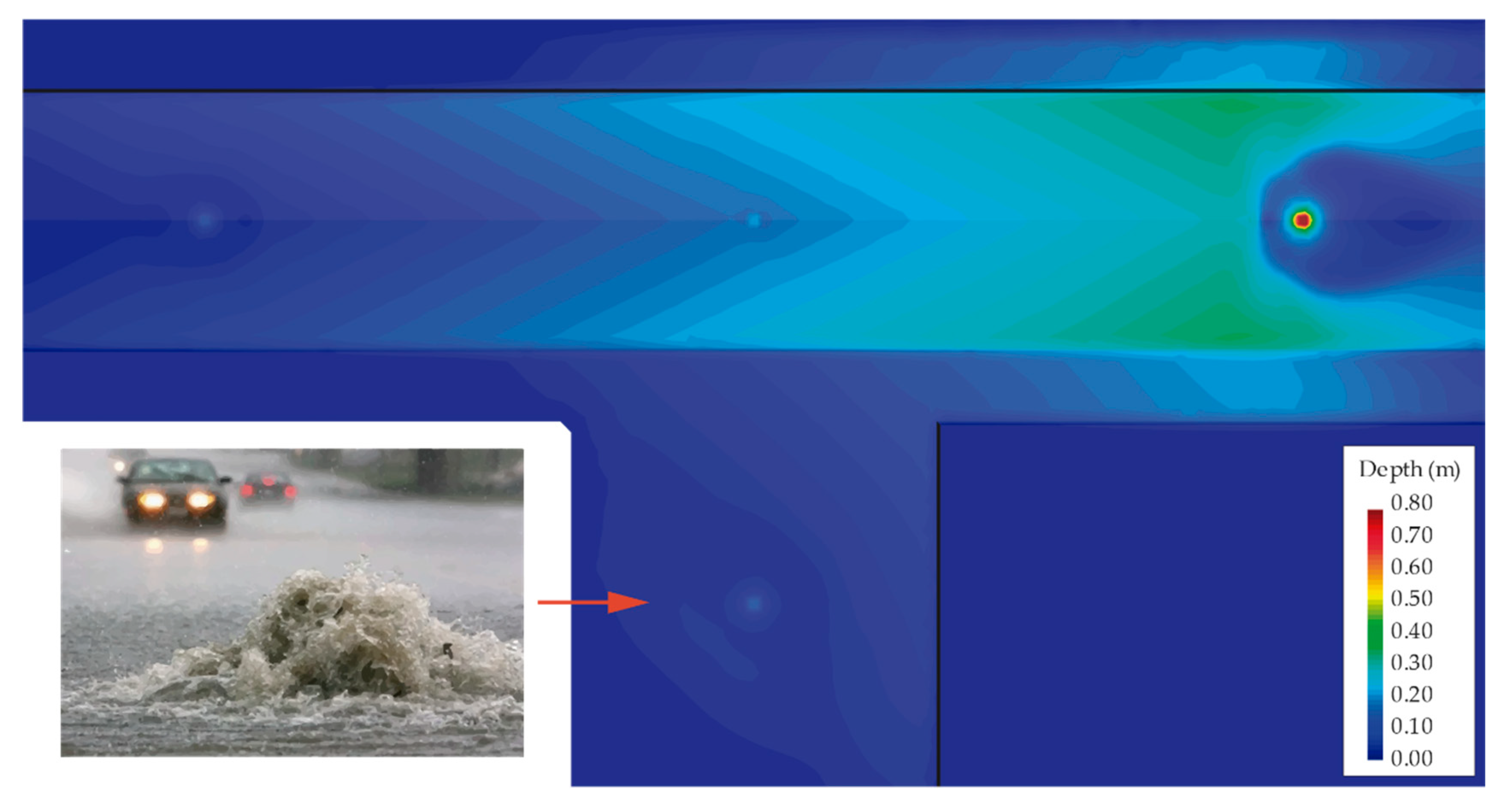
Figure 4 shows the evolution of water depths and discharges at the four manholes. At all the manholes, the water depth increases slowly during the first 60 min, due to the rainfall input and to the water coming from the imposed hydrographs at manholes M1 and M4. At that time, the sudden rise of the downstream boundary hydraulic head condition triggers a sharp increase in the manhole depths. Once their maximum depth is exceeded, the water flows outside the manhole and into the street surface. Figure 5 shows the computed maximum water depths in the street surface. It can be seen the water column that typically occurs when flooding from manholes.
The effect of rainfall alone is not enough to trigger the surface flooding in this case. However, the rainfall runoff allows to check for this case study the behaviour of the inlets before the flooding occurs. Figure 6a shows the volume of water intercepted by inlets and roofs. It can be noticed how, once the flooding occurs (approximately at minute 60), the inlets stop catching water.
In order to verify the global mass conservation of the coupled model, including the surface and sewer models as well as the linking methodology, the mass balance error was computed at each time step of the simulation as
where is the precipitation volume, is the overland flow storage, is the volume intercepted by the inlets, is the volume intercepted by the roofs, is the outlet volume through the domain boundaries, is the infiltration volume, and is the volume that returns to the surface through the manholes. The relative accumulated mass balance error in relation with the outlet boundary volume is at every time step lower than 1% (Figure 6b).
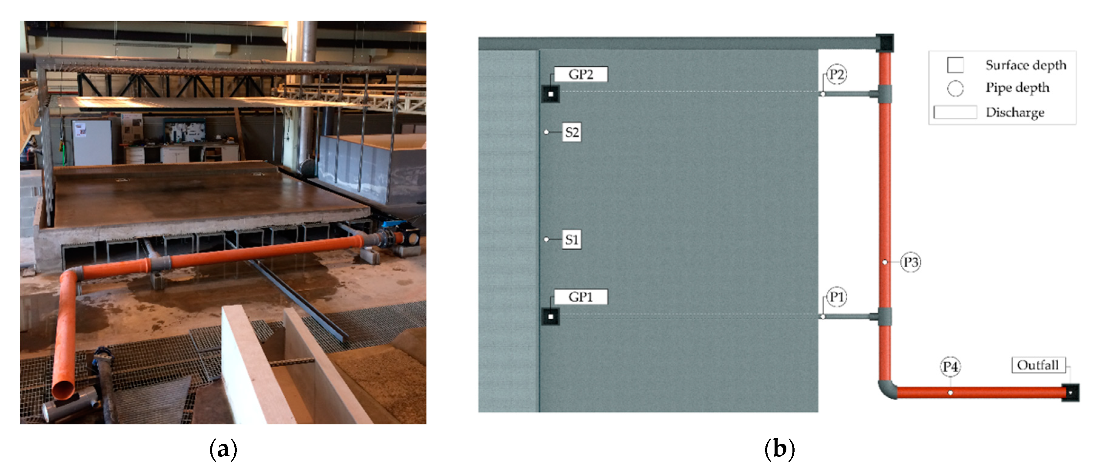
3.2. Full-Scale Urban Drainage Physical Model
3.2.1. Case Study Description
This case presents the experimental validation of the dual drainage model using a set of laboratory data obtained in a real scale physical model. The physical model consists of a full-scale street section of 36 m2 with a sewer system and a rainfall simulator. This facility was used in previous studies [10,35,36,37] to validate urban drainage models and to measure wash-off and sediment transport in urban environments. The street consists of a concrete roadway and a concrete pavement separated by a 15-cm high curb. The roadway has 2% and 0.5% transversal and longitudinal slopes, respectively. Surface runoff is drained through two inlets and through a lateral channel that ends into a third inlet. From there, water is conveyed through the sewer system to a downstream outfall (Figure 7). The street geometry and experimental data presented in WASHTREET [38] were used to build the numerical model.
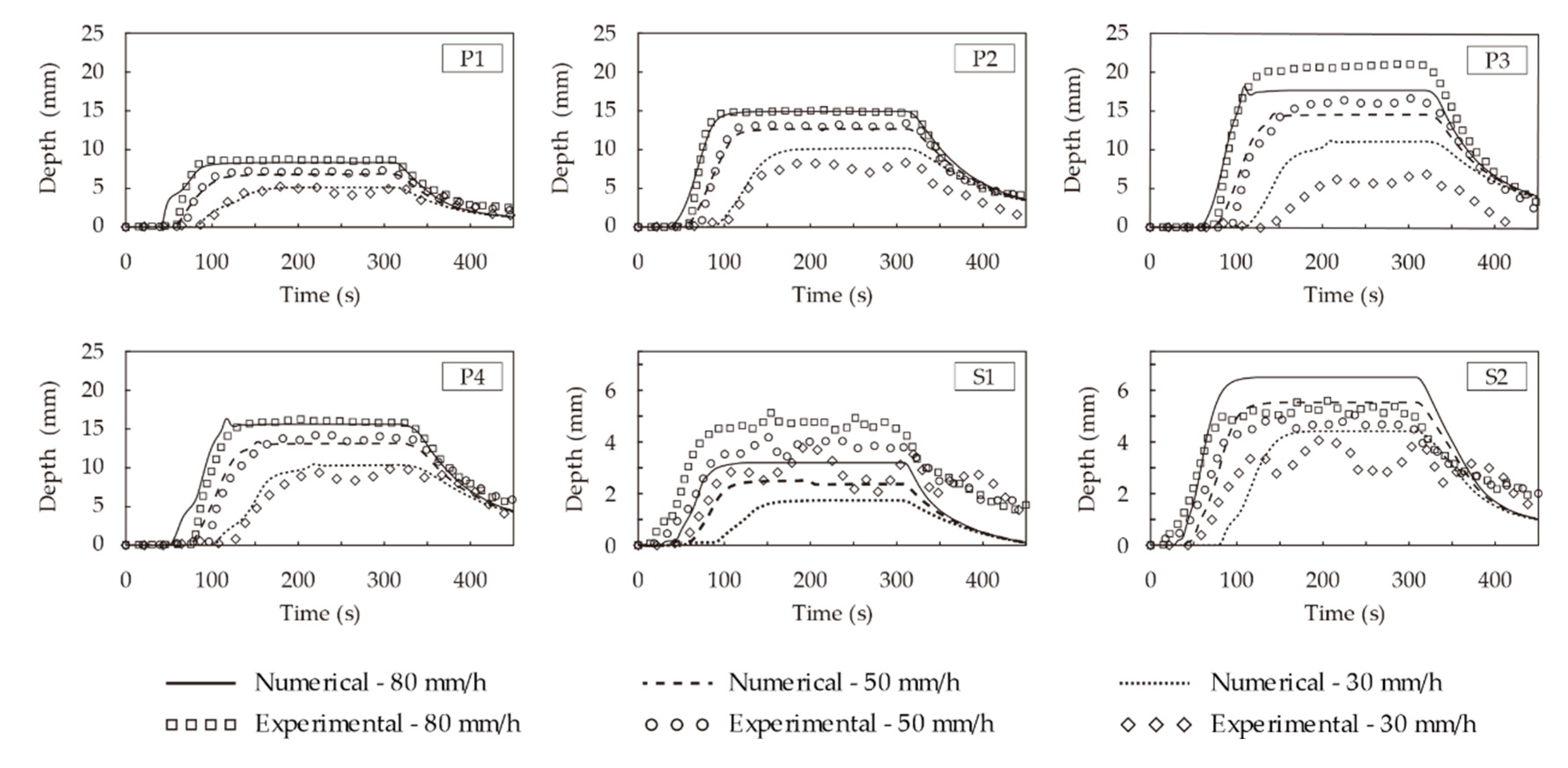
Three different rainfall intensities of 30, 50 and 80 mm/h were simulated. In order to compare the experimental data with the numerical results, the hydraulic variables in a set of control points were analysed (Figure 7b). The water discharges through the two inner inlets and at the outfall were compared. In addition, the water depth at 6 locations within the pipes and at 3 surface control points were compared.
The surface domain was discretized using an unstructured mesh with an average element size of 0.06 m and approximately 20,000 elements. From previous studies in this laboratory facility [36], the Manning coefficient was set to 0.016, and an initial abstraction of 0.6 mm was established in the whole surface. In the lateral plastic channel and in all the pipes of the sewer network, the Manning coefficient was set to 0.008 [10].
3.2.2. Results
Figure 8 shows the experimental and numerical hydrographs computed at the two inlets and at the outfall for the three rainfall intensities. The numerical and experimental data present a good agreement at both inlets being the mean absolute error (MAE) less than 0.01 L/s for all the rainfall intensities. Regarding the agreement at the outfall, a small-time lag between the numerical and experimental data can be observed during the rising limb of the hydrographs (MAE less than 0.09 L/s). This difference is due to the way in which the outfall discharge was measured in the experimental tests. Experimental discharge was measured in a deposit located at the end of the sewer network that produced a slight lamination of the experimental hydrograph [37].
Figure 9 shows the water depths at pipes and at the surface. The results present a reasonable agreement at all the control points, specially at P1, P2 and P4, being the MAE less than 1 mm for all the rainfall intensities except for P2 and intensity 30 mm/h that is 2 mm. P3 present less agreement being the maximum MAE 3.5 mm. Notice that the water depth at those control points is very low in relation to the diameter of the pipe, so a minimum difference between the real and modelled geometry can significantly affect the results. The same happens at the surface control points, where the measured water depths are extremely small, and thus, the effect of the microtopography and other physical phenomena that are no considerer in the numerical model, such as drop impacts, can have an effect on the numerical-experimental agreement. Nonetheless, the numerical model simulates the surface water depths and its temporal dynamics with a reasonable agreement (MAE always less than 1.5 mm).
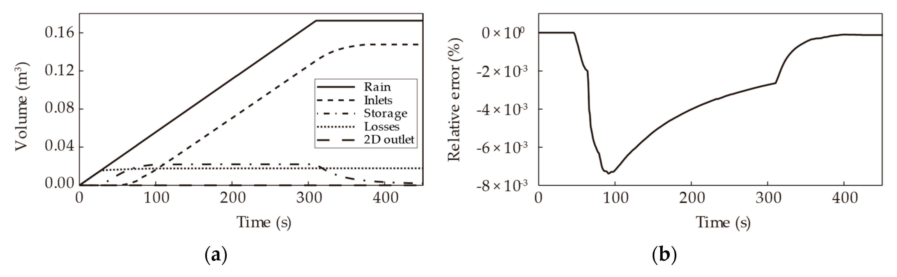
Finally, Figure 10a shows the water volumes computed during the simulation. Most of the rainfall volume is drained through the inlets. Using the mass conservation Equation (5), the mean mass conservation error during the whole simulation in relation with the precipitation volume is 0.003% and tends to zero at the end of simulation (Figure 10b).
3.3. Real Urban Settlement
3.3.1. Case Study Description
The last case study shows the application of the dual drainage model to El Rubio, an urban settlement located in Andalucía (Spain) with a population of 3500 inhabitants. The workflow needed to import the sewer network from a GIS data base using external free tools is also detailed.
The urban area was split in two different regions according to the different land uses: an urban impervious region and a pervious region. The available digital terrain model (DTM), which has a resolution of 2 m, and other geometric information such as the layout of buildings and infiltration areas are shown in Figure 11. Due to the lack of field data that could be used to calibrate the model parameters, the Manning coefficient was set to 0.016 in the urban area and to 0.20 in the rest of the domain [39,40]. The SCS Curve Number Method was used to compute infiltration losses. Based on the GCN250 dataset [41], a curve-number (CN) of 75 was imposed for all the pervious areas, while the urban domain was considered to be completely impervious. The spatial domain included in the computations includes all the surrounding terrains that drain into the urban region, in order to consider the surface runoff coming from upstream areas.
The sewer system (Figure 11b) is composed of 727 manholes, 753 links and 3 outfalls. The information of the sewer system was provided in GIS data format, so it was necessary to convert it to the SWMM input format. To do so, the R software package swmmr was used. The R package swmmr is a free tool that contains specific functions to read and write SWMM files, run SWMM simulations from R and convert SWMM input files to and from GIS data [42]. The inlets were not included in the SWMM input file. Thus, all the inlets that do not have an associated manhole in the GIS data are automatically assigned by the model to the nearest manhole. Unlike in the two previous case studies, the DTM available for this case has a limited resolution (2 m), which means that the pathlines of water at the streets could not be resolved with an enough resolution to direct the water towards the inlets. Other methodologies to catch overland flow when the topography does not have enough resolution, such as the definition of a density of inlets in a micro-catchment that drains into a manhole [33], will be analysed in future works.
In order to evaluate the effect of the numerical discretisation on the results, two different computational meshes with different spatial resolution were used to discretize the domain. The coarse mesh has 100,000 elements and an average element size of 10 m, while the fine mesh has 1,000,000 elements, with an average element size of 2 m inside the urban area and of 20 m in the rest of the domain.
3.3.2. Results
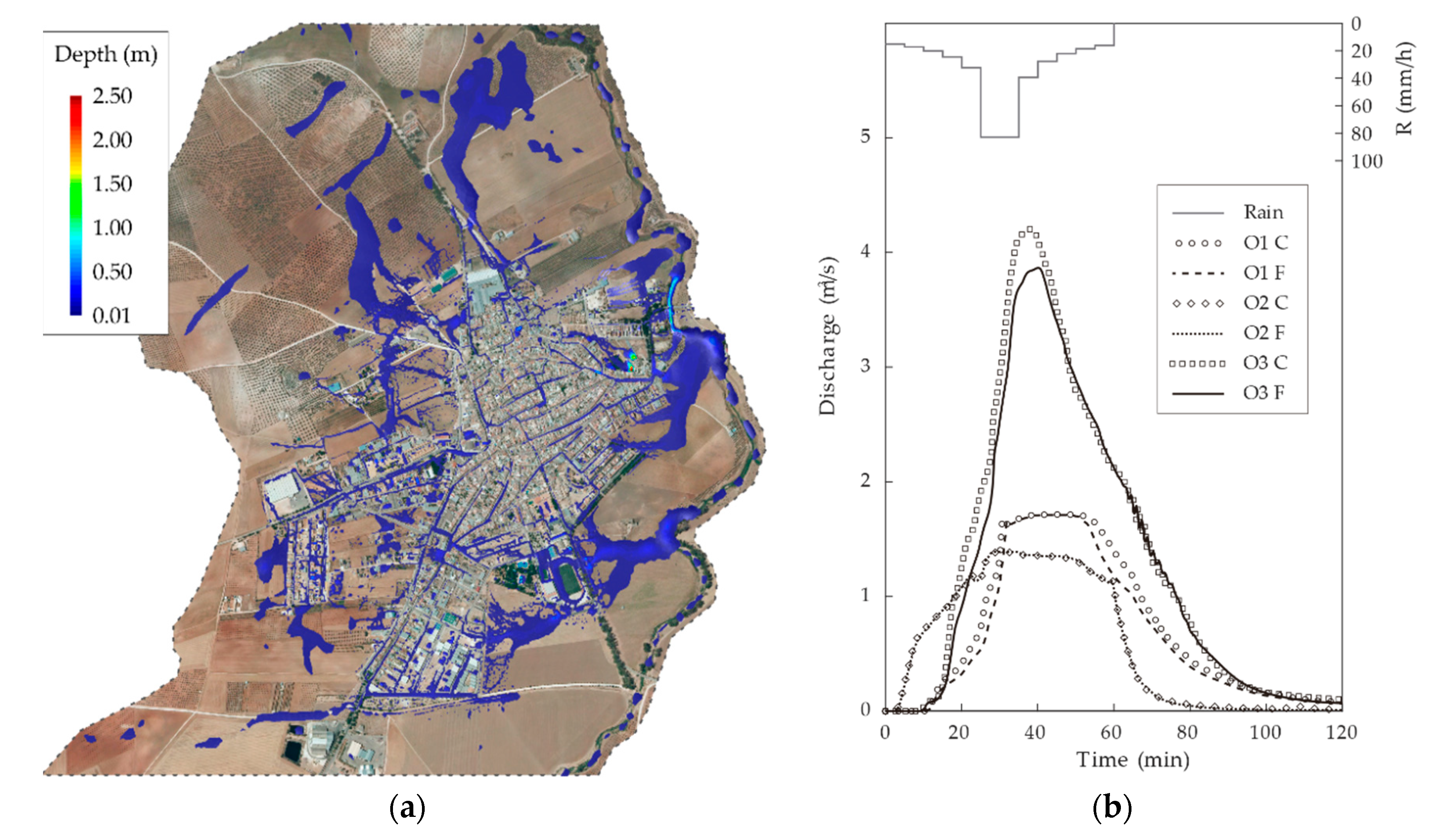
Figure 12a shows the spatial distribution of the maximum water depth computed during the simulation with the fine mesh. To facilitate the visualization of the results, water depths lower than 0.01 m are not represented. The results obtained with the coarse mesh are very similar and are therefore not shown in the figure.
Figure 12b shows the discharges at the three outfalls (see location in Figure 11b) computed with the fine and coarse meshes. The hydrographs computed at outfall O2 with both meshes are virtually the same (MAE of 0.01 m3/s). At outfall O1, there are some minor differences at some time steps, but those are not significant for practical purposes (MAE of 0.06 m3/s), and the peak discharge computed with both meshes is the same. Regarding outfall O3, the MAE increases to 0.11 m3/s, and the difference in peak discharge is around 8%. While these differences are larger than in the case of O1 and O2, they are still small for the analysis of sewer networks in real applications, where the uncertainties on input data are in general larger than those values. Moreover, it should be considered that the CPU time was 15 times larger when using the fine mesh in relation to the coarse mesh.
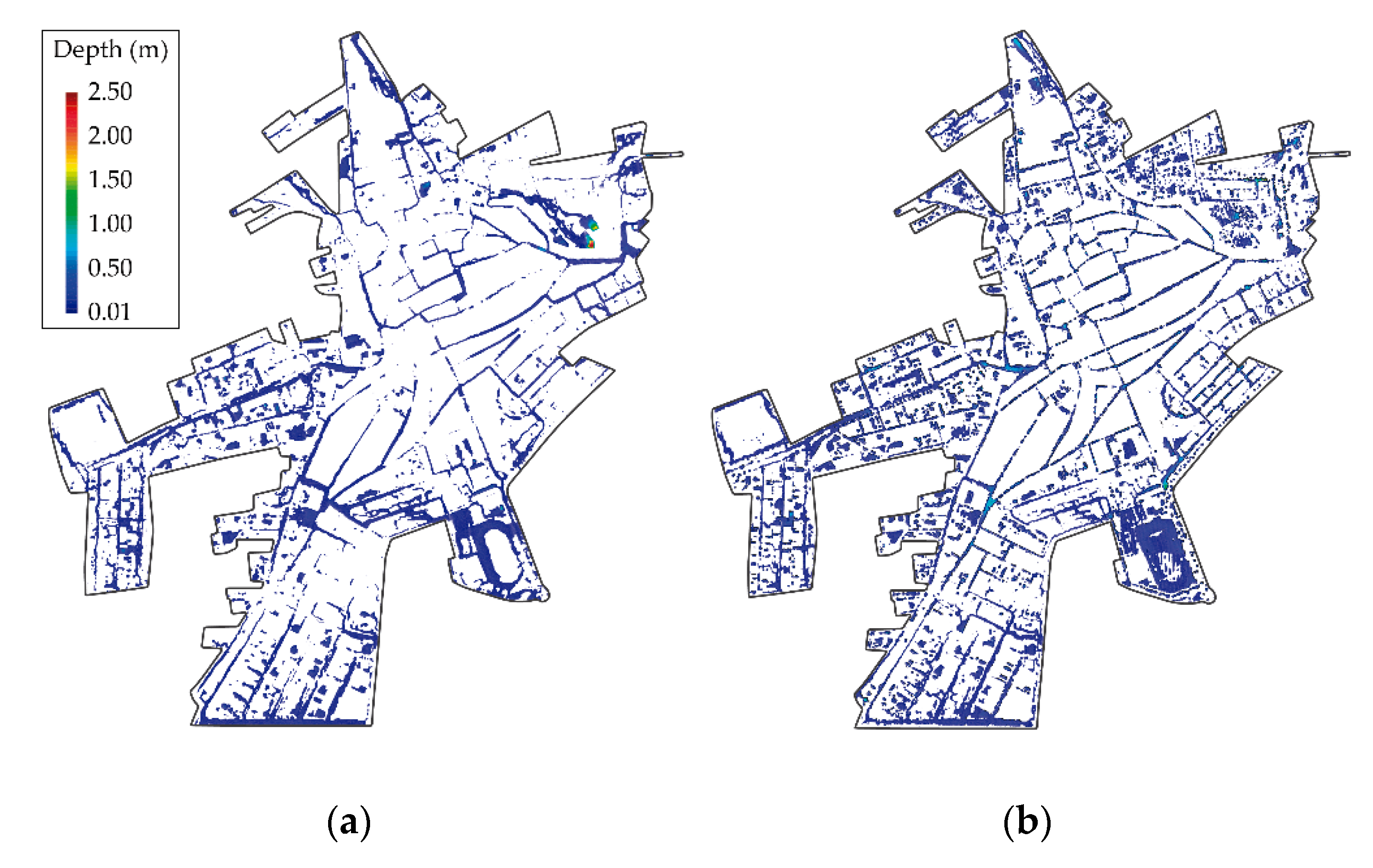
A simulation without the sewer network was carried out in order to highlight the role of the sewer drainage system during a rainfall event. Figure 13 shows the maps of maximum depth during the rainfall event considering and not considering the sewer network in the model. The results are shown only in the urban impervious area, and the building shapes were removed from the figure in order to facilitate the visualization. The extension of the flood is significantly different, being, as expected, bigger for the case without sewer network, which corroborates the essential role that play the sewer network systems during extreme rainfall events. Thus, the no consideration of the sewer network implies a 10% and 35% of increase in the depths and in the flood extension, respectively.
4. Conclusions
A 1D/2D dual drainage model linking two free distributed hydraulic models (Iber and SWMM) was presented. The model allows the simulation of water flow in the surface and sewer drainage networks, including their bidirectional interaction. The linking methodology computes the discharge transferred from the surface to the sewer network, and vice versa, at each computational time step and is based in a SWMM-DLL library that contains different functions to interact with SWMM before, during and after the simulation.
The capabilities of the model were shown in three case studies at different spatial scales. The first case study was used to validate the basic capabilities of the model and to show its suitability to compute surface flooding conditions caused by the surcharge of the sewer network. In the second case study, the numerical results are compared against experimental data obtained in a full-scale urban drainage physical model. Finally, the third case was used to show the capability of the model to simulate pluvial floods in real urban settlements, incorporating the available GIS data of the sewer system.
Further developments of the model will include different methodologies to compute the transfers of water captured by inlets and roofs, the implementation of SuDS (Sustainable Drainage System) techniques and the enhancement of the computational time. In addition, future works will also compare the present model with other well-known dual drainage models, in order to analyse its capabilities and its advantages and disadvantages against these.
Author Contributions
Conceptualization, L.C., J.P. and E.S.; methodology, L.C., J.P. and E.S.; software development, E.S.; supervision software development, L.C. and J.P.; validation, E.S.; writing—original draft preparation, E.S.; writing—review and editing, L.C. and J.P.; supervision, L.C. and J.P. All authors have read and agreed to the published version of the manuscript.
Funding
The contract of the first author is funded by the INTERREG ATLANTIC AREA program through the project AA-FLOODS Enhanced Prevention, Warning, Coordination and Emergency Management Tools for Floods at Local Scales (EAPA_45/2018).
Acknowledgments
The authors acknowledge ARECIAR and CMAOT for supplying, respectively, the sewer network information and the topographic data of the third test case.
Conflicts of Interest
The authors declare no conflict of interest. The funders had no role in the design of the study; in the collection, analyses or interpretation of data; in the writing of the manuscript or in the decision to publish the results.
References
- Cea, L.; Garrido, M.; Puertas, J.; Jácome, A.; Del Río, H.; Suárez, J. Overland flow computations in urban and industrial catchments from direct precipitation data using a two-dimensional shallow water model. Water Sci. Technol. 2010, 62, 1998–2008. [Google Scholar] [CrossRef]
- Fraga, I.; Cea, L.; Puertas, J.; Suarez, J.; Jimenez, V.; Jacome, A. Global sensitivity and GLUE-Based uncertainty analysis of a 2D-1D dual urban drainage model. J. Hydrol. Eng. 2016, 21. [Google Scholar] [CrossRef]
- Chen, A.S.; Leandro, J.; Djordjević, S. Modelling sewer discharge via displacement of manhole covers during flood events using 1D/2D SIPSON/P-DWave dual drainage simulations. Urban Water J. 2016, 13, 830–840. [Google Scholar] [CrossRef] [Green Version]
- Martins, R.; Leandro, J.; Chen, A.S.; Djordjević, S. A comparison of three dual drainage models: Shallow water vs local inertial vs diffusive wave. J. Hydroinform. 2017, 19, 331–348. [Google Scholar] [CrossRef] [Green Version]
- Djordjević, S.; Prodanović, D.; Maksimović, Č. An approach to simulation of dual drainage. Water Sci. Technol. 1999, 39, 95–103. [Google Scholar] [CrossRef]
- Leandro, J.; Chen, A.S.; Djordjevi, S.; Savi, D.A. Comparison of 1D/1D and 1D/2D coupled (Sewer/Surface) hydraulic models for urban flood simulation. J. Hydraul. Eng. 2009, 135, 495–504. [Google Scholar] [CrossRef]
- Fraga Cadórniga, I. Desarrollo de un modelo dual 1D/2D para el cálculo del drenaje urbano: Modelo numérico y validación experimental. Ph.D. Thesis, Universidade da Coruña, A Coruña, Spain, 2015. [Google Scholar]
- Aragón-Hernández, J.L. Modelación numérica integrada de los procesos hidráulicos en el drenaje urbano. Ph.D. Thesis, Universitat Politècnica de Catalunya, Barcelona, Spain, 2013. [Google Scholar]
- Leandro, J.; Martins, R. A methodology for linking 2D overland flow models with the sewer network model SWMM 5.1 based on dynamic link libraries. Water Sci. Technol. 2016, 73, 3017–3026. [Google Scholar] [CrossRef]
- Fraga, I.; Cea, L.; Puertas, J. Validation of a 1D-2D dual drainage model under unsteady part-full and surcharged sewer conditions. Urban Water J. 2017, 14, 74–84. [Google Scholar] [CrossRef]
- Rossman, L.A. Storm Water Management Model User’s Manual Version 5.1.; EPA/600/R-14/413b; National Risk Management Research Laboratory, Office of Research and Development, U.S. Environmental Protection Agency: Cincinnati, OH, USA, 2015; p. 352.
- Hsu, M.H.; Chen, S.H.; Chang, T.J. Dynamic inundation simulation of storm water interaction between sewer system and overland flows. J. Chin. Inst. Eng. Trans. Chin. Inst. Eng. Ser. A Chung Kuo K. Ch’eng Hsuch K’an 2002, 25, 171–177. [Google Scholar] [CrossRef] [Green Version]
- Pathirana, A.; Tsegaye, S.; Gersonius, B.; Vairavamoorthy, K. A simple 2-D inundation model for incorporating flood damage in urban drainage planning. Hydrol. Earth Syst. Sci. 2011, 15, 2747–2761. [Google Scholar] [CrossRef] [Green Version]
- Jahanbazi, M.; Egger, U. Application and comparison of two different dual drainage models to assess urban flooding. Urban Water J. 2014, 11, 584–595. [Google Scholar] [CrossRef]
- Kim, S.E.; Lee, S.; Kim, D.; Song, C.G. Stormwater inundation analysis in small and medium cities for the climate change using EPA-SWMM and HDM-2D. J. Coast. Res. 2018, 85, 991–995. [Google Scholar] [CrossRef]
- Martins, R.; Leandro, J.; Djordjević, S. Influence of sewer network models on urban flood damage assessment based on coupled 1D/2D models. J. Flood Risk Manag. 2018, 11, S717–S728. [Google Scholar] [CrossRef]
- Adeogun, A.G.; Pathirana, A.; Daramola, M.O. Others 1D-2D hydrodynamic model coupling for inundation analysis of sewer overflow. JEAS J. Eng. Appl. Sci. 2012, 7, 356–362. [Google Scholar] [CrossRef] [Green Version]
- Delelegn, S.W.; Pathirana, A.; Gersonius, B.; Adeogun, A.G.; Vairavamoorthy, K. Multi-objective optimisation of cost-benefit of urban flood management using a 1D2D coupled model. Water Sci. Technol. 2011, 63, 1053–1059. [Google Scholar] [CrossRef] [PubMed]
- Seyoum, S.D.; Vojinovic, Z.; Price, R.K.; Weesakul, S. Coupled 1D and noninertia 2D flood inundation model for simulation of urban flooding. J. Hydraul. Eng. 2012, 138, 23–34. [Google Scholar] [CrossRef]
- Phillips, B.C.; Yu, S.; Thompson, G.R.; Silva, N. De 1D and 2D Modelling of Urban Drainage Systems using XP-SWMM and TUFLOW. In Proceedings of the 10th International Conference on Urban Drainage, Copenhagen, Denmark, 21–26 August 2005. [Google Scholar]
- Bisht, D.S.; Chatterjee, C.; Kalakoti, S.; Upadhyay, P.; Sahoo, M.; Panda, A. Modeling urban floods and drainage using SWMM and MIKE URBAN: A case study. Nat. Hazards 2016, 84, 749–776. [Google Scholar] [CrossRef]
- SWMM5 Modeling with PCSWMM. Available online: https://www.pcswmm.com/ (accessed on 6 September 2020).
- Bladé, E.; Cea, L.; Corestein, G.; Escolano, E.; Puertas, J.; Vázquez-Cendón, E.; Dolz, J.; Coll, A. Iber: Herramienta de simulación numérica del flujo en ríos. Rev. Int. Metod. Numer. Calc. Disen. Ing. 2014, 30, 1–10. [Google Scholar] [CrossRef] [Green Version]
- SWMM-Docs: Open Water Analytics Stormwater Management Model. Available online: http://wateranalytics.org/Stormwater-Management-Model/index.html (accessed on 17 July 2020).
- Bladé Castellet, E.; Cea, L.; Corestein, G. Numerical modelling of river inundations. Ing. Agua 2014, 18, 68. [Google Scholar] [CrossRef]
- Cea, L.; Bladé, E. A simple and efficient unstructured finite volume scheme for solving the shallow water equations in overland flow applications. J. Am. Water Resour. Assoc. 2015, 5, 2. [Google Scholar] [CrossRef] [Green Version]
- García-Feal, O.; González-Cao, J.; Gómez-Gesteira, M.; Cea, L.; Domínguez, J.M.; Formella, A. An accelerated tool for flood modelling based on Iber. Water 2018, 10, 1459. [Google Scholar] [CrossRef] [Green Version]
- Fraga, I.; Cea, L.; Puertas, J. Effect of rainfall uncertainty on the performance of physically based rainfall–runoff models. Hydrol. Process. 2019, 33, 160–173. [Google Scholar] [CrossRef] [Green Version]
- Cea, L.; Legout, C.; Darboux, F.; Esteves, M.; Nord, G. Experimental validation of a 2D overland flow model using high resolution water depth and velocity data. J. Hydrol. 2014, 513, 142–153. [Google Scholar] [CrossRef]
- Rossman, L.A. Storm Water Management Model Reference Manual Volume II—Hydraulics; U.S. Environmental Protection Agency: Washington, DC, USA, 2017.
- Chen, A.S.; Djordjević, S.; Leandro, J.; Savić, D.A. The urban inundation model with bidirectional flow interaction between 2D overland surface and 1D sewer networks. Novatech 2007 2007, 465–472. [Google Scholar]
- Lopes, P.; Leandro, J.; Carvalho, R.F.; Páscoa, P.; Martins, R. Numerical and experimental investigation of a gully under surcharge conditions. Urban Water J. 2015, 12, 468–476. [Google Scholar] [CrossRef]
- Gómez, M.; Russo, B. Methodology to estimate hydraulic efficiency of drain inlets. Proc. Inst. Civ. Eng. Water Manag. 2011, 164, 81–90. [Google Scholar] [CrossRef]
- Flood risk management. Engineering. University of Exeter. Available online: https://emps.exeter.ac.uk/engineering/research/cws/research/flood-risk/rapids.html (accessed on 30 July 2020).
- Naves, J. Wash-off and Sediment Transport Experiments in a Full-Scale Urban Drainage Physical Model. Ph.D. Thesis, Universidade da Coruña, A Coruña, Spain, 2019. [Google Scholar]
- Naves, J.; Anta, J.; Puertas, J.; Regueiro-Picallo, M.; Suárez, J. Using a 2D shallow water model to assess Large-Scale Particle Image Velocimetry (LSPIV) and Structure from Motion (SfM) techniques in a street-scale urban drainage physical model. J. Hydrol. 2019, 575, 54–65. [Google Scholar] [CrossRef]
- Naves, J.; Anta, J.; Suárez, J.; Puertas, J. Hydraulic, wash-off and sediment transport experiments in a full-scale urban drainage physical model. Sci. Data 2020, 7, 1–13. [Google Scholar] [CrossRef]
- Naves, J.; Anta, J.; Suárez, J.; Puertas, J. Washtreet—Hydraulic, wash-off and sediment transport experimental data obtained in an urban drainage physical model. Sci. Data 2019. [Google Scholar] [CrossRef]
- Cea, L.; Legout, C.; Grangeon, T.; Nord, G. Impact of model simplifications on soil erosion predictions: Application of the GLUE methodology to a distributed event-based model at the hillslope scale. Hydrol. Process. 2016, 30, 1096–1113. [Google Scholar] [CrossRef]
- Fraga, I.; Cea, L.; Puertas, J. Experimental study of the water depth and rainfall intensity effects on the bed roughness coefficient used in distributed urban drainage models. J. Hydrol. 2013, 505, 266–275. [Google Scholar] [CrossRef]
- Jaafar, H.H.; Ahmad, F.A.; Beyrouthy, N. El GCN250, new global gridded curve numbers for hydrologic modeling and design. Sci. Data 2019, 1–9. [Google Scholar] [CrossRef] [Green Version]
- Leutnant, D.; Döring, A.; Uhl, M. Swmmr—An R package to interface SWMM. Urban Water J. 2019, 16, 68–76. [Google Scholar] [CrossRef] [Green Version]
- Arias, J.S. Máximas Lluvias Diarias en España Peninsular; Seria Monográfica del Ministerio de Fomento: Madrid, Spain, 1999; p. 55. [Google Scholar]
Figure 1.
Flow diagram of the 1D/2D urban drainage model.

Figure 2.
(a) Scheme of the urban street; (b) boundary conditions at manholes and outfall.

Figure 3.
Longitudinal profile of the drainage network.

Figure 4.
Results of depths and discharges at manholes and maximum water depth for manholes.

Figure 5.
Results of maximum depths at surface and photography of a manhole flooding [34] that justifies the assumption that the main returned flow to the surface occurs through the manholes.
Figure 5.
Results of maximum depths at surface and photography of a manhole flooding [34] that justifies the assumption that the main returned flow to the surface occurs through the manholes.

Figure 6.
(a) Time series evolution of accumulative volumes; (b) mass balance error during the simulation for the simplified urban street.
Figure 6.
(a) Time series evolution of accumulative volumes; (b) mass balance error during the simulation for the simplified urban street.

Figure 7.
(a) Physical model facility and (b) measuring points in inlets, pipes and surfaces used for results validation.
Figure 7.
(a) Physical model facility and (b) measuring points in inlets, pipes and surfaces used for results validation.

Figure 8.
Experimental and numerical profiles of discharges at inlets GP1 (left) and GP2 (middle) and at the outfall (right).
Figure 8.
Experimental and numerical profiles of discharges at inlets GP1 (left) and GP2 (middle) and at the outfall (right).

Figure 9.
Experimental and numerical profiles of depths in pipes at control points P1 (top-left), P2 (top-middle), P3 (top-right) and P4 (bottom-left) and in surface at control points S1 (bottom-middle) and S2 (bottom-right).
Figure 9.
Experimental and numerical profiles of depths in pipes at control points P1 (top-left), P2 (top-middle), P3 (top-right) and P4 (bottom-left) and in surface at control points S1 (bottom-middle) and S2 (bottom-right).

Figure 10.
(a) Time series evolution of accumulative volumes; (b) mass balance error during the simulation for full-scale urban drainage physical model.
Figure 10.
(a) Time series evolution of accumulative volumes; (b) mass balance error during the simulation for full-scale urban drainage physical model.

Figure 11.
(a) DEM of the study area; (b) sewer network of the urban settlement.

Figure 12.
(a) Maximum depths at surface; (b) numerical hydrographs computed at outfalls for a 1 h design storm with a 25-year return period for coarse (C) and fine (F) mesh.
Figure 12.
(a) Maximum depths at surface; (b) numerical hydrographs computed at outfalls for a 1 h design storm with a 25-year return period for coarse (C) and fine (F) mesh.

Figure 13.
Maximum depths on the surface: (a) with and (b) without considering the sewer network.

© 2020 by the authors. Licensee MDPI, Basel, Switzerland. This article is an open access article distributed under the terms and conditions of the Creative Commons Attribution (CC BY) license (http://creativecommons.org/licenses/by/4.0/).
Share and Cite
MDPI and ACS Style
Sañudo, E.; Cea, L.; Puertas, J. Modelling Pluvial Flooding in Urban Areas Coupling the Models Iber and SWMM. Water 2020, 12, 2647. https://doi.org/10.3390/w12092647
AMA Style
Sañudo E, Cea L, Puertas J. Modelling Pluvial Flooding in Urban Areas Coupling the Models Iber and SWMM. Water. 2020; 12(9):2647. https://doi.org/10.3390/w12092647
Chicago/Turabian StyleSañudo, Esteban, Luis Cea, and Jerónimo Puertas. 2020. "Modelling Pluvial Flooding in Urban Areas Coupling the Models Iber and SWMM" Water 12, no. 9: 2647. https://doi.org/10.3390/w12092647
Note that from the first issue of 2016, this journal uses article numbers instead of page numbers. See further details here.