Dynamic Evaluation of Sustainable Water Resource Systems in Metropolitan Areas: A Case Study of the Beijing Megacity

Abstract

Increasing water scarcity has made it difficult to meet global water demands, so the sustainable use of water resources is an important issue. In this study, the sustainable water resource system (SWRS) operating mechanism is discussed, considering three components: dynamics, resistance and coordination. According to the SWRS operating mechanism, a universal indicator system with three layers, including goal, criterion, and index layers, is constructed for SWRS evaluation. Additionally, considering the fuzziness of threshold values for grading standards, an SWRS evaluation model is constructed based on the set pair analysis (SPA), analytic hierarchy process (AHP) and attribute interval recognition methods. This model is conceptually simple and convenient. An evaluation indicator system is constructed for the SWRS in Beijing, and evaluation standards with five grades are established. The dynamics of the sustainability of the Beijing SWRS and corresponding operating mechanism are analyzed using the SPA evaluation model. The results suggest that the three components of the operating mechanism all have positive effects on the Beijing SWRS state, but the SWRS state has not yet been fundamentally changed. Therefore, considerable improvements can be achieved regarding the sustainability of the Beijing SWRS.

1. Introduction

Economic growth, industrial development, human health, food security and ecosystems are all water-dependent [1]. Since the 1980s, global water use has been growing by approximately 1% yearly, and this trend has been mainly caused by population growth, socioeconomic development and evolving consumption patterns [2,3]. The global water demand is forecasted to continue to increase at a similar rate until 2050, accounting for an increase of 20 to 30% overall [4], mainly due to the increases in demand of the industrial and domestic sectors [4,5,6]. The water stress level will continue to increase as the demand for water growth, the uncertainty of the water supply and the effects of climate change intensify. Therefore, sustainable development and the management of water resources are very important and for human survival and development.

Studies on the sustainability of water development and management have been popular since the concept of sustainable development was first proposed in a World Commission on the Environment and Development report [7]. Sustainability is a concept that describes the dynamic conditions of complex systems, in particular, the biosphere of the Earth and the socioeconomic systems within it [8]. Initially, many studies focused on the sustainability of hydrological systems. Concepts such as renewability and the carrying capacity of the hydrological cycle in a basin were adopted to measure the relative sustainability of water resources for human appropriation [9,10,11]. Fresh water in nature has become a resource associated with socioeconomic development. Water resources have not only natural value but also social, economic and ecological functions. Hence, a water resource system is a complex system of coupled natural hydrological systems, ecosystems and socioeconomic systems [12]. Scholars have studied this complex water resource system, defined the sustainability of water resource system, and assessed the sustainability criteria, measured the extent to which systems are sustainable, developed evaluation index systems and methods, and established management policies and regulations. For example, Feng (1991) defined a water resource system as being composed of a number of interrelated and interactive water resources components associated with different management and technical units [13]. Loucks (1997) defined sustainable water resource systems (SWRSs) as those that are designed and managed to contribute to societal objectives at present and at the future while maintaining ecological, environmental and hydrological integrity [10]. In the book “Sustainable Criteria for Water Resources Systems”, Loucks (1999) illustrated the economic, ecological and environmental sustainability criteria related to water resource management and planning and offered possible solutions for achieving sustainable development with respect to water resource systems [14]. To assess the sustainability of water resources, a conceptual framework and practical tools for integrated assessment have been outlined in some studies. Water sustainability indexes (reliability, resilience and vulnerability) are used to assess the sustainability of a water resource system and identify key factors for improving the sustainability of the system [15,16,17,18]. Koop and van Leeuwen (2015) used the city blueprint indicators to assess the sustainability of the city water resources [19]. Zhang et al. (2018) proposed an assessment method based on relative entropy in information entropy theory to accurately reflect the sustainability of regional water resources in various areas [20]. A system dynamics approach was employed to simulate the sustainability of a water resource system to provide a basis for management policy and decision-making [21,22]. Sun et al. (2016) established indicators to evaluate the sustainability of water utilization based on the Drive–Pressure–Status–Impact–Response (DPSIR) model [23]. Later, many scholars constructed indicator systems at different levels by using multicriteria methods to evaluate the sustainability of water resource systems in many basins, regions and cities [24,25,26,27,28,29,30]. Although these methods define a water resource system as a complex system composed of different subsystems (e.g., the water subsystem, socioeconomic subsystem, and ecological subsystem), these subsystems are treated independently in the construction of evaluation indicator systems, thus lacking the interlinkages among different subsystems with different mechanisms.

The United Nations World Water Development Report 2019 indicated that more than 2 billion people live in areas of high water stress [31]. Nearly all net population growth takes place in urban areas and increasing urbanization has generated new and difficult challenges for city water resource management. Currently, over half (54%) of the global population lives in cities and the global urban population is expected to increase to two-thirds of the global population [32]. Sustainable water development challenges will therefore continue in cities. In this context, the Beijing megacity is used as an example, and the operating mechanisms and dynamics of the water resource system (SWRS), are investigated. This study attempts to (1) analyze an SWRS and the corresponding operating mechanism based on sustainability theory and system science perspectives, (2) establish an universal evaluation indicator system for the SWRS based on the operating mechanism, (3) construct an assessment model with an SWRS based on the set pair analysis (SPA) method and analytic hierarchy process (AHP) method and (4) analyze the sustainability and dynamics of the SWRS in the Beijing megacity. This study provides new insights into the operating mechanisms and sustainability of water resource systems in megacities.

2. Study Area

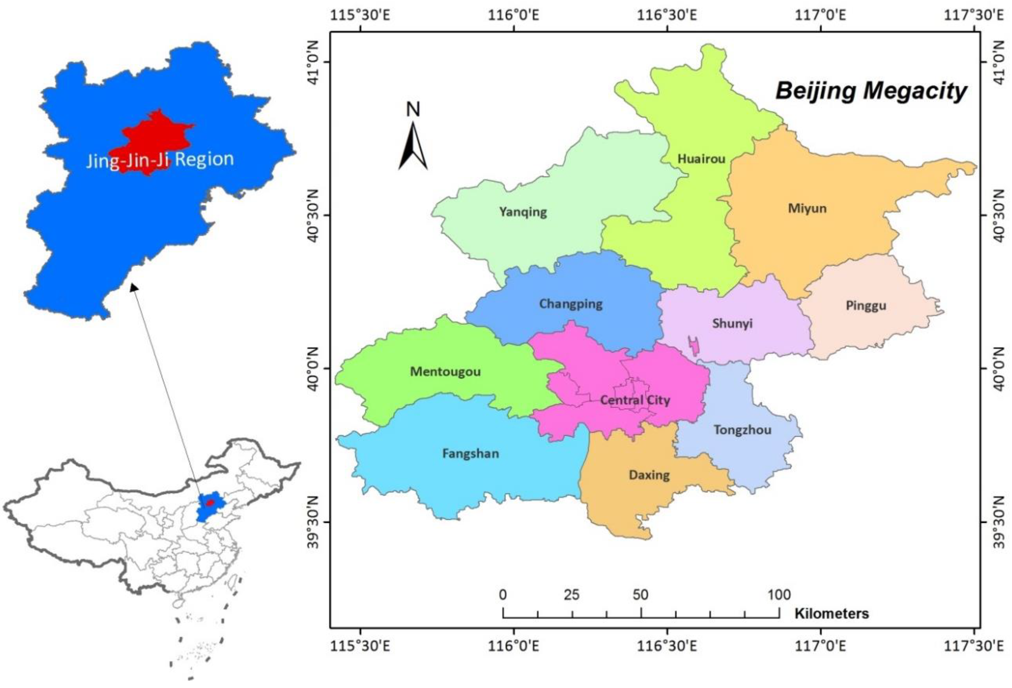
Beijing is the capital of the People’s Republic of China and is one of the four province-level municipalities in China. The Beijing municipality consists of 16 districts, which cover an area of 16,410.54 km² (Figure 1). Nestled on the north of the North China Plain, Beijing borders Tianjin Municipality to the east and Hebei Province in all other directions. Beijing, Tianjin and Hebei have formed a new economic community called the Jing-Jin-Ji region (Figure 1). In 2019, Beijing’s GDP was greater than CNY 3500 billion, an increase of 6.1% over that in the previous year. Additionally, as of 2019, the permanent resident population of the city was 21.536 million, the urban population was 18.65 million and the rural population was 2.886 million. The urban population accounted for 86.6% of the city’s permanent residents.

Beijing is high in the northwest and low in the southeast. The city is surrounded by mountains to the west, north and northeast. To the southeast, the North China Plain gradually descends towards the Bohai Sea. Mountain areas occupy approximately 62% of the municipality’s total area. Five major waterways flow from west to east through the municipality: the Juma, Yongding, Beiyun, Chaobai and Jiyun Rivers. Beijing has a temperate, continental monsoonal climate, characterized by short spring and autumn seasons, hot and rainy summers, and cold and dry winters. The average annual temperature is 11 to 14 °C. The average annual precipitation in the area is 585 mm, and the heaviest rainfall occurs in June, July and August, accounting for approximately 80% of the total annual precipitation.

Although Beijing’s per capita GDP is very high, reaching approximately CNY 165,000/person (or USD 24,000/person) in 2019, the per capita local water resources in Beijing are very low at only ~140 m³/person. Water resource shortages have become one of the critical factors hindering the sustainable development of the Beijing megacity. Therefore, evaluations of water resources sustainability in Beijing can be used to diagnose and understand SWRS conditions and dynamics in Beijing in terms of the operating mechanisms.

3. Theory and Methods

3.1. Operating Mechanism of an SWRS

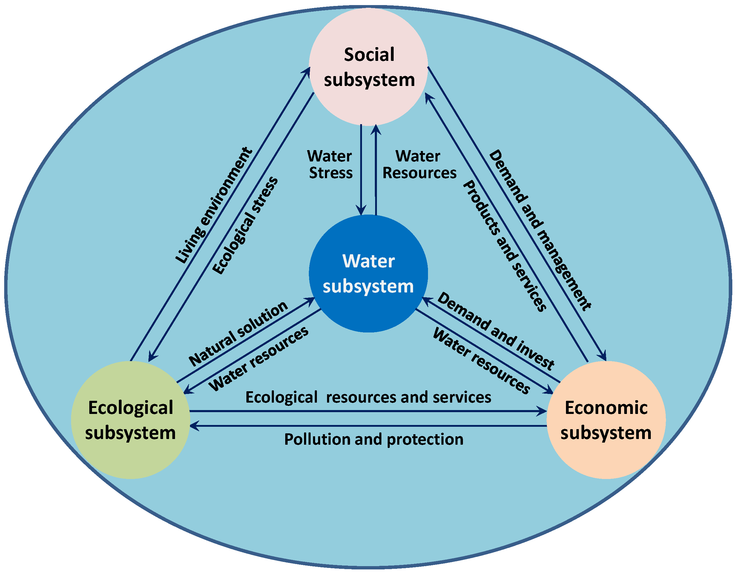
An SWRS is an open and complex megasystem involving natural water systems (e.g., the hydrological cycle subsystem and ecological subsystem), human social systems (e.g., the social subsystem, economic subsystem, and hydraulic engineering subsystem) and management and service systems (e.g., the water conservancy technology subsystem, evaluation and criterion subsystem, and management and regulation subsystem). Water sustainability has been defined as a dynamic state of water supply and use that meets societal needs without compromising the long-term capacity of the water system to meet the needs of future generations [33]. An SWRS is a complex coupled system with a water resource system as the core; such a system integrates social, economic and eco-environment subsystems that interact with each other and continuously evolve in time and space. An SWRS can maintain an environmental balance, promote the integrity of hydrological processes and meets the current and future needs of sustainable socioeconomic development by using hydraulic engineering, technological and other measures to protect and allocate water resources in a way that establishes harmony among humans, water and nature. An SWRS is controlled and affected by the water resource system, social system, economic system and eco-environmental system (Figure 2).

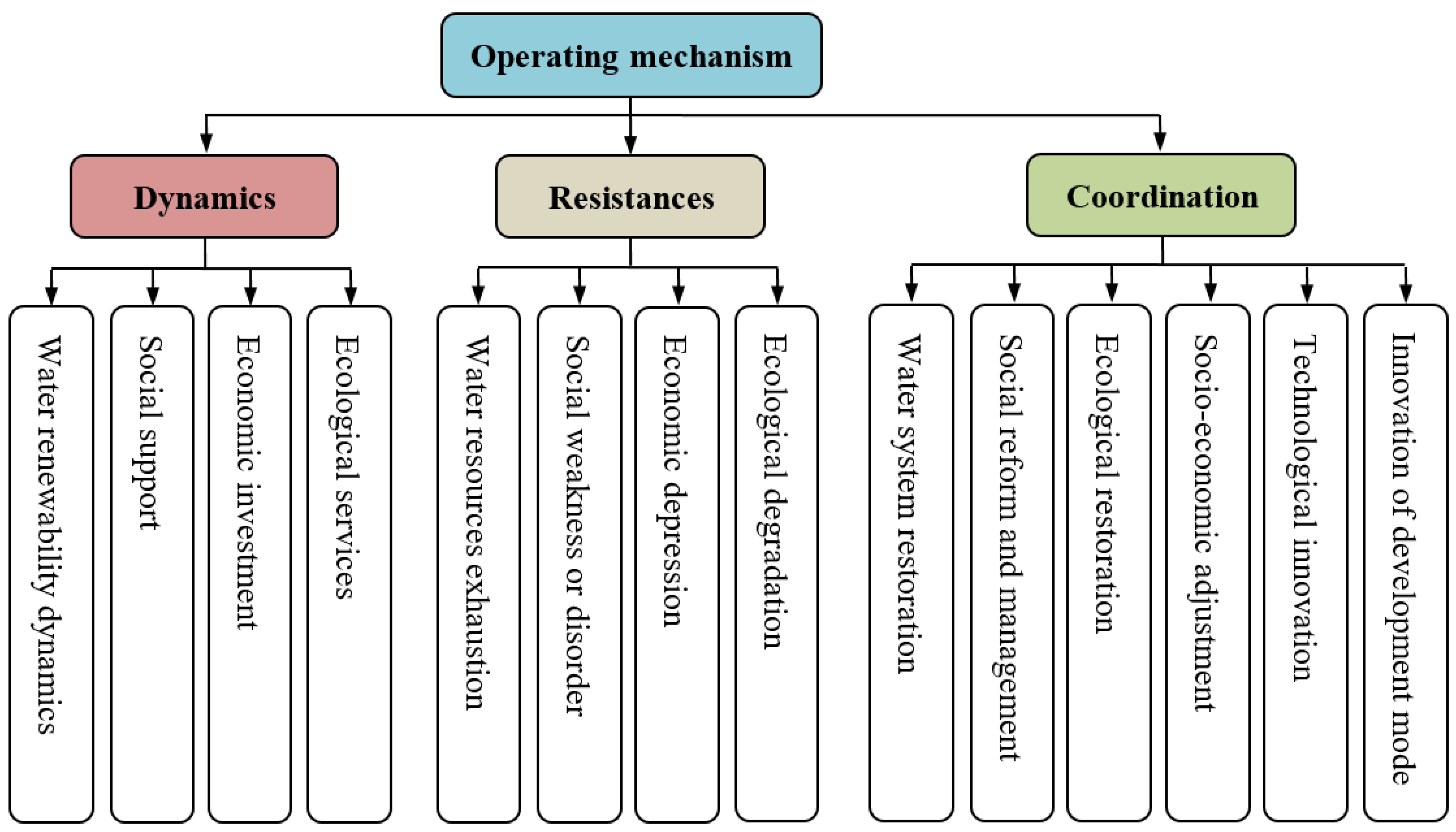
Mechanisms are the interactions and interlinkages among the specific elements (society, economy, resources, and environment) and abstract elements (information, interests, rights, and goals) of a system and they maintain order and coordination among subsystems [35]. Driving forces are necessary to maintain the operation of a system. However, every coin has two sides, and there must be a resistance factor to hinder the development of a system. For a system to overcome resistance factors and maintain healthily and sustainably operations, a system must have coordinated functionality. Similarly, for a sustainable water resource system to operate in a sustainable and healthy way, dynamic, resistant and coordinated attributes are necessary: these factors represent the three major operating mechanisms of an SWRS (Figure 3). The dynamic mechanism provides driving forces for the continuous development of an SWRS. The resistance mechanism hinders the positive evolution of an SWRS via interference or consumption. The coordination mechanism plays an important role in adjusting or correcting the operating direction of an SWRS via feedback. These three mechanisms are mutually restricted and coordinated, and all are important.

For an SWRS, the dynamic mechanism includes three components: the renewable dynamics of water resources, the socioeconomic support dynamics and the dynamics of ecological services. The resistance mechanism includes the resistances related to water scarcity, economic depression, social instability and ecological degradation, and the coordination mechanism involves water system restoration, socioeconomic adjustment and ecological restoration. These mechanisms together determine the direction and modes of an SWRS.

3.2. Indicator System of an SWRS

In the past, sustainable indexes (e.g., the carrying capacity, vulnerability and reliability) were often used to measure the sustainability of water resource development and utilization [10,11,30,36]. However, these indexes can only be used to describe the state of an SWRS and fail to explain the causes of SWRS changes in terms of the corresponding mechanism. This study attempts to construct a universal indicator system according to the operation mechanism of an SWRS and its components. The indicator system is divided into three layers: goal, criterion and index layers. The indicator in a goal layer is the SWRS condition. The criterion layer contains indicators for the dynamic condition, resistance condition and coordination condition, which correspond to the three major mechanisms of the SWRS. The indicators in the index layer are generated according to the system dynamics, resistance and coordination.

In

Table 1. Universal evaluation indicator system for an SWRS.

Goal Layer (A)	Criterion Layer (B)	Index Layer (C)	Unit
SWRS conditions	B1. Dynamic conditions	C1. Drought index	(-)
		C2. Annual precipitation	mm/year
		C3. Runoff depth	mm
		C4. Runoff yield modulus	m3/km2
		C5. Groundwater modulus	m3/km2
		C6. Per capita water resources	m3/person
		C7. Population density	person/km2
		C8. Urbanization rate	%
		C9. Per capita gross domestic product (GDP)	CNY/person
		C10. Proportion of investment in water projects	%
		C11. Industrialization rate	%
		C12. Forest coverage	%
		C13. Stream connectivity	(-)
	B2. Resistance conditions	C14. Water resource development ratio	%
		C15. Per capita water use	m3/person
		C16. Proportion of agricultural water use	%
		C17. Proportion of industrial water use	%
		C18. Proportion of ecological water use	%
		C19. Leakage rate of municipal networks	%
		C20. Groundwater overexploitation ratio	%
		C21. Proportion of saltwater intrusion area	%
		C22. Proportion of soil erosion area	%
		C23. Desertification rate	%
		C24. Proportion of sewage discharge	%
	B3. Coordination conditions	C25. Water consumption in GDP per 10,000 CNY	m3/CNY
		C26. Irrigation water per unit area	m3/hm2
		C27. Wastewater treatment ratio	%
		C28. Groundwater recharge ratio	%
		C29. Proportion of water transfer	%
		C30. Proportion of rainwater utilization	%
		C31. Proportion of water supply by reclaimed water	%
		C32. Water price	CNY/m3
		C33. Investment ratio of ecological restoration	%

, the indicators corresponding to each index in the criterion layer all involve the water subsystem, social subsystem, economic subsystem and ecological subsystem, and they correspond to the components of each mechanism of an SWRS. Indicators C1–C33 have physical meaning and are available. Due to space limitations, the meaning of and measurement method for each indicator are not explained individually here. This indicator system is applicable to SWRS evaluation in most regions. However, an indicator system for a certain region needs to be modified considering the actual situation in and features of the region.

According to the operation mechanism of an SWRS and the corresponding universal indicator system, the evaluation indicator system of the Beijing SWRS was divided into three layers, namely, the goal, criterion and index layers, as shown in

Table 2. Evaluation indicator system for the Beijing SWRS.

Goal Layer (A)	Criterion Layer (B)	Index Layer (C)	Unit	Symbol
SWR Cconditions	B1. Dynamic conditions	C11. Annual precipitation	mm	+
		C12. Per capita local water resources	m3/P	+
		C13. Per capita GDP	CNY/P	+
		C14. Urbanization rate	%	+
		C15. Forest coverage	%	+
	B2. Resistance conditions	C21. Water resource development ratio	%	-
		C22. Proportion of domestic water consumption	%	-
		C23. Proportion of agricultural water use	%	-
		C24. Proportion of industrial water use	%	-
		C25. Proportion of water supply to eco-environment	%	+
		C26. Proportion of sewage discharge	%	+
	B3. Coordination conditions	C31. Proportion of water consumption in the GDP per 10,000 CNY	m3/CNY	-
		C32. Per capita daily domestic water use	L/(P·d)	-
		C33. Water use in Industry value added per 10,000 CNY	m3/CNY	-
		C34. Irrigation water per unit area	m3/hm2	-
		C35. Wastewater treatment ratio	%	+
		C36. Proportion of water supplied by water transfer projects	%	+
		C37. Proportion of water supplied by reclaimed water	%	+
		C38. Urban greenery coverage	%	+

Note: “+” means that the greater the indicator value is, the better the performance is, and “-” has the opposite meaning.

. The goal layer only includes one indicator, The Beijing SWRS condition (A), which is described by the goal connection degree calculated based on the weighted connection degrees of indicators for the criterion layer. The criterion layer includes three indicators, namely, the dynamic conditions (B1), resistance conditions (B2) and coordination conditions (B3), which correspond to the dynamic, resistance and coordination components of the operating mechanism of the Beijing SWRS.

In the index layer, five indicators are used to describe the dynamic component of the operating mechanism of the Beijing SWRS; annual precipitation (C11), the per capita local water resources (C12), the per capita GDP (C13), the urbanization rate (C14) and forest coverage (C15). C11 reflects the status and renewability of water resources in the Beijing region. C12 reflects the extent to which the Beijing megacity has access to freshwater resources. C13 indicates the potential economic support for the available water resources. C14 reflects the social development level, which affects the mode and efficiency of water resource utilization. C15 represents the positive support of ecological conditions for water resource conservation in the Beijing region.

Six indicators that encompass the resistance mechanism are selected in the index layer and they include the water resource development rate (C21), proportion of domestic water consumption (C22), proportion of agricultural water use (C23), proportion of industrial water use (C24), proportion of water supply to the eco-environment (C25), and proportion of sewage discharge (C26). C21 describes the overall extent of water resources in the Beijing megacity. C22, C23 and C24 represent the extent of water consumption and the increased pressure on the water subsystem caused by the socioeconomic development in Beijing, respectively. C25 and C26 represent the eco-environmental pressure caused by water resource exploitation and conservation activities.

Eight indicators are selected to evaluate the coordination performance of the Beijing SWRS. The proportion of water consumption in the GDP per 10,000 CNY (C31) is a comprehensive indicator that represents the socioeconomic outcome directly tied to water resources, and the overall efficiency of water resource utilization increases with this indicator. C32, C33 C34 and C35 are indicators that reflect the efficiency of water consumption for different industries. Because the water transferred to Beijing and available rainwater resources increases, the pressure on the water supply system decreases. Hence, proportions of the south to north water diversion project (C36) and reclaimed water (C37) are considered to coordinate the contradiction between water consumption and the supply of the water subsystem. C38 (urban greenery coverage) is selected to describe the contribution of urban ecological conservation to water system restoration and a healthy living environment.

3.3. Set Pair Analysis Model of an SWRS

Generally, specific index values are used as grade standards to evaluate problems related to water resources. For example, a water reuse rate of 90% is used as the dividing value of evaluation grades 1 and 2. If the measured water reuse is 91%, the evaluation is classified as grade 1. However, if the value is 89%, the result is classified as grade 2. Obviously, the rigid evaluation standard fails to consider the fuzzy problem of indicator values and ignores the identity, discrepancy and contradistinction relations between two neighboring grades. This study adopts a new SPA method to the above issues; the SPA method was originally proposed by Zhao (2000) [37].

The principle of SPA assumes that (i) the set pair for two relative sets in an uncertain system is constructed; (ii) the properties of the two sets are expressed by the identity, discrepancy and contradistinction; (iii) the connection degree of a set pair can be calculated. Set pair construction is the basis of SPA, and the connection degree is the key results in this method [38].

Set A and relative set B form a set pair H = (A, B); n terms in A = (a₁, a₂, …, a_n) and in B = (b₁, b₂, …, b_n) are used to show the characteristics of set A and set B, respectively. s is the number of identical terms for a given characteristic, p is the number of contradictory terms, and f = n-s-p is the number of discrepant terms [37].

$${\mu }_{A-B}=\frac{s}{n}+\frac{f}{n}i+\frac{p}{n}j$$

(1)

where μ_A−B ∈ [−1,1] is the connection degree of H = (A, B). Let a = s/n, b = f/n, and c = p/n, a, b, c ∈ [0, 1] are the identity degree, discrepancy degree and contradistinction degree, respectively, where a + b + c = 1. i is the uncertainty coefficient of the discrepancy, and this value ranges between −1 and 1. j is the uncertainty coefficient of the contradistinction degree, which has a value of −1 or can be considered a marker of contradistinction in some cases.

Equation (1) is the general expression of the three-element connection degree. A new expression for an n-element connection degree can be obtained by expanding the discrepancy degree (b) in Equation (1) to b₁i₁ + b₂i₂ + … + b_n−2i_n−2. The n-element connection degree can be obtained as

$${\mu }_{A-B}=a+b_1{i}_1+b_2{i}_2+\cdots +b_{n-2}{i}_{n-2}+cj$$

(2)

where a + b₁ + b₂ + … + b_n−2 + c = 1 and b₁, b₂ … b_n−2 are the components of the discrepancy degree corresponding to different grades. i₁, i₂ … i_n−2 are the uncertainty variables and coefficients of the discrepancy degree.

In this study, the indicator system is divided into three layers. Parameter A represents the indicator (SWRS condition) in the goal layer. B_p represents the p-th indicator in the criterion layer. C_pq represents the q-th evaluation index of the p-th criterion index. If the evaluation standard values for the indicator system are classified into n grades, the n-element connection degree of each indicator can be calculated using Equation (2). The specific expressions of connection degrees for each layer are detailed in Appendix A. It should be noted that the weight of indicators should be considered for the criterion layer and the goal layer. In this study, the indicator weights are determined by using the AHP method.

3.4. Indicator Weight Determination

The contributions and influences of different indicators to the SWRS are different. Hence, each indicator needs to be assigned a weight to describe its role in the SWRS. This study adopts the AHP method to determine the weights of indicators in the criterion layer and the index layer [39]. The steps of the method are (1) to determine the importance of the indicators to the overall objective by pairwise comparison; (2) to estimate the relative weights of indicators using the “eigenvalue” method; (3) to assess the consistency of the comparison matrix using the consistency index.

In this case, indicators C11–C15 in Table 2 are used as an example to illustrate the weight calculation. First, a comparison matrix used to describe the relative importance of each indicator is constructed by assigning an objective or subjective assignment of preference weights based on a pairwise comparison scale (1–9) (

Table 3. The analytic hierarchy process (AHP) pairwise comparison scale.

Degree of Importance	Definition
1	Both indicators equally important
3	Very slight importance of one indicator over the other
5	Moderate importance of one indicator over the other
7	Demonstrated importance of one indicator over the other
9	Extreme or absolute importance of one indicator over the other
2, 4, 6, and 8	Intermediate values between two adjacent judgments

). For example, if indicator C11 is moderately important compared to indicator C12, the relative importance of C11 over C12 is valued at 5 and that of C12 over C11 is valued at 1/5. The comparison matrix A = (a_ij) is obtained by a pairwise comparison of indicators C11–C15, as shown in

Table 4. Pairwise comparisons of indicators C11–C15.

	C11	C12	C13	C14	C15
C11	1	5	7	7	3
C12	1/5	1	5	5	2
C13	1/7	1/5	1	1	1/3
C14	1/7	1/5	1	1	1/3
C15	1/3	1/2	3	3	1

. The principal diagonal of the matrix contains entries of 1 because each factor is as important as itself.

The next step is to calculate the maximum eigenvalue of the comparison matrix and the corresponding eigenvector. The entries in each column of the matrix are summed (A_j = ∑_i(a_ij), where i and j are the row and column labels, respectively). Each entry of a column is divided by that sum, namely a_ij/A_j, and a new normalized matrix is obtained (A’ = (a’_ij) = (a_ij/A_j), where i, j = 1, 2, 3, 4, and 5). The entries in each row of matrix A’ are summed to obtain a column vector (A’_i = ∑_j(a’_ij)). The eigenvector ω of the comparison matrix A is calculated by dividing A’_i by the sum of the entries of the normalized matrix (∑a’_ij). The normalized matrix and the eigenvector are listed in

Table 5. The normalized matrix and the eigenvector.

	C11	C12	C13	C14	C15	ω
C11	0.55	0.72	0.41	0.41	0.45	0.51
C12	0.11	0.14	0.29	0.29	0.3	0.23
C13	0.08	0.03	0.06	0.06	0.05	0.06
C14	0.08	0.03	0.06	0.06	0.05	0.06
C15	0.18	0.07	0.18	0.18	0.15	0.15

. According to A ω = λ_max ω, the maximum eigenvalue (λ_max) of the comparison matrix A is determined, namely λ_max = A ω/ω = 5.20.

Finally, the consistency index (CI) and consistency ratio (CR) are employed to assess the consistency of the comparison matrix. The consistency index for an n × n matrix with maximum eigenvalue λ_max is CI = (λ_max − n)/(n − 1). RI is the consistency index for a randomly generated n × n matrix. Using the CI and RI, the consistency ratio is defined as CR = CI/RI. Values of CR ≤ 0.1 are desired. High CR values imply unacceptable inconsistency, and respondents were asked to revise their pairwise comparison ratings in such cases. In this example, the order (n) of matrix A is 5, and CI = (λ_max − n)/(n−1) = (5.20 − 5)/(5 − 1) = 0.05. The RI for 5 × 5 matrix A is 1.12, and CR = 0.05/1.12 = 0.046 < 0.1, which is acceptable for the consistency test of the comparison matrix. Hence, the eigenvector corresponding to λ_max contains the weights of C11–C15, namely, ω = (0.51, 0.23, 0.06, 0.06, 0.15).

4. Results and Discussions

4.1. Evaluation Results for the Index Layer

The values of these indicators (C11–C38) in Table 2 are available from the Beijing Water Resources Bulletin (2000–2018) [40], Beijing Water Statistical Yearbook (2016–2018) [41] and Beijing Statistical Yearbook (2019) [42], as shown in

Table 6. The indicator values in the index layer of the indicator system of the Beijing SWRS.

Indicator	2000	2001	2002	2003	2004	2005	2006	2007	2008	2009	2010	2011	2012	2013	2014	2015	2016	2017	2018
C11 (mm)	438	462	413	453	539	468	448	499	638	448	524	552	708	501	439	583	660	592	590
C12 (m3/P)	123.6	138.6	113.2	126.3	143.0	150.7	137.9	142.1	193.2	117.4	117.6	132.8	190.9	117.3	94.1	123.3	161.4	137.1	164.6
C13 (CNY/P)	24,518	27,430	31,307	35,450	41,809	47,127	52,964	61,470	66,098	68,406	75,573	83,547	89,778	97,178	102,869	109,603	118,198	128,994	140,211
C14 (%)	77.5	78.1	78.6	79.1	79.5	83.6	84.3	84.5	84.9	85.0	86.0	86.2	86.2	86.3	86.4	86.5	86.5	86.5	86.5
C15 (%)	29.0	30.5	31.6	33.1	34.5	35.3	35.9	36.5	36.5	36.7	37.0	37.6	38.6	40.1	41.0	41.6	42.3	43.0	43.5
C21 (%)	240.2	202.8	214.9	183.4	152.3	137.6	139.1	125.4	83.0	120.9	111.8	98.5	64.8	100.4	138.8	78.8	58.2	67.9	54.1
C22 (%)	32.1	31.0	31.3	36.3	37.0	38.8	39.9	39.9	41.9	41.4	41.8	43.3	44.6	44.8	45.3	45.8	45.9	46.3	46.8
C23 (%)	40.8	44.7	44.6	38.5	39.1	38.3	37.3	35.7	34.2	33.8	32.4	30.3	25.9	25.0	21.9	17.0	15.7	12.9	10.7
C24 (%)	26.0	23.6	21.8	23.5	22.2	19.7	18.1	16.5	14.8	14.6	14.5	13.9	13.6	14.0	13.6	9.9	9.8	8.9	8.4
C25 (%)	1.1	0.8	2.3	1.7	1.8	3.2	4.7	7.8	9.1	10.1	11.4	12.5	15.9	16.2	19.2	27.2	28.6	31.9	34.1
C26 (%)	57.7	64.2	74.4	61.3	62.6	56.0	64.8	66.1	66.3	68.6	71.6	70.6	72.7	72.6	73.1	77.0	78.7	85.9	94.0
C31 (m3/CNY)	125.7	103.3	78.8	70.1	56.0	48.3	41.3	34.6	30.8	28.6	24.4	21.7	19.6	17.9	17.1	16.1	15.1	14.1	13.0
C32 (L/(P·d))	260.4	238.3	208.5	244.6	234.6	238.3	234.4	227.1	227.4	216.5	205.3	211.7	211.8	211.2	216.5	220.9	224.4	231.0	234.0
C33 (m3/CNY)	123.2	96.9	73.0	67.9	48.7	39.3	33.4	27.2	23.9	22.1	18.1	16.1	14.5	13.9	13.2	9.9	9.4	8.2	7.4
C34 (m3/hm2)	3632.2	4578.9	4611.9	4584.7	4440.8	4292.2	3993.8	4216.9	3726.7	3750.0	3593.2	3597.4	3286.2	3760.3	4100.8	3680.0	4039.7	4047.6	3962.3
C35 (%)	39.4	42	45	50.1	53.9	62.4	73.2	76.2	78.9	80.3	81	82	83	84.6	86.1	87.9	90	92.4	93.4
C36 (%)	0.0	0.0	0.0	0.0	0.0	0.0	0.0	0.0	2.1	11.9	11.3	9.7	7.1	14.8	4.1	32.9	30.3	36.2	33.6
C37 (%)	0.0	0.0	0.0	11.1	9.6	10.3	16.4	20.8	17.5	29.8	29.5	26.5	19.0	32.3	42.8	35.4	28.6	35.3	30.4
C38 (%)	36.5	38.2	40.2	40.87	41.91	42	42.5	43	43.5	44.4	45	45.6	46.2	46.8	47.4	48	48.4	48.42	48.44

.

The rationality of the indicator standards directly affects the accuracy of the Beijing SWRS evaluation. For the principle of grading, a five-grade standard division is adopted based on the relevant regulations of the state (

Table 7. The grading standards for the indicators in the index layer for the Beijing SWRS.

Indicator	Grade 1 (Very Poor)	Grade 2 (Poor)	Grade 3 (Medium)	Grade 4 (Good)	Grade 5 (Excellent)
C11 (mm)	200	400	800	1600	3000
C12 (m3/P)	500	1000	2000	3000	5000
C13 (CNY/P)	5000	15,000	40,000	120,000	300,000
C14 (%)	20	40	50	60	80
C15 (%)	10	20	35	50	60
C21 (%)	60	40	30	20	10
C22 (%)	50	40	25	15	8
C23 (%)	80	70	50	40	20
C24 (%)	30	25	20	15	10
C25 (%)	1	2	3.5	10	20
C26 (%)	20	30	50	70	90
C31 (m3/CNY)	300	150	60	40	20
C32 (L/(P·d))	200	180	150	120	100
C33 (m3/CNY)	250	200	120	80	60
C34 (%)	6500	6000	5500	4500	3000
C35 (m3/hm2)	20	40	60	80	90
C36 (%)	10	20	30	40	60
C37 (%)	10	20	30	40	50
C38 (%)	10	20	30	50	70

). In general, the standards for these indicators are identified with reference to (1) the oval global situation and (2) the overall situation in China. Here, only indicators C11–C15 are used as an example to illustrate how the standards are determined. The annual precipitation distribution in China varies from below 50 to above 3000 mm [43], and the standards of C11 are determined to have five grades. According to the internationally recognized water shortage standards (<3000 m³, mild; <2000 m³, moderate; <1000 m³, severe, and <500 m³, extreme) and the per capita water resources in China (~2000 m³), the five grades of C12 are divided as shown in Table 7. According to the global per capita water resources in the Word Bank dataset [44], the dividing point values for the grades 1–5 for C13 are set as 300,000, 120,000, 40,000, 15,000, and 5000. The C14 and C15 standards are set based on the urbanization levels in developing and developed countries around the world [32] and the forest coverage of the countries [44]. Due to space limitations, other indicators will not be described in detail here. The grading standards are shown in Table 4.

According to the principle of SPA, the values of indicators for the index, criterion and goal layers form set A, and the standard values of the five grades for these indicators form set B. These two sets are combined to obtain the set pair H(A, B). The connection degrees of the set pair H(A, B) can be calculated using Equations (2), (A1) and (A2). Since the connectivity degree ranges from −1 to 1, a different grading scale is used to effectively depict the evaluation results. According to the SPA model, the connection degrees approaching 1 indicate excellent evaluation results. In contrast, the evaluation is poor when the connection degree is close to −1. Corresponding to the standard of the indicators in the index system of the SWRS (five grades), the evaluation standard for the connection degrees of the three layers is divided into five grades: very poor (grade 1), poor (grade 2), medium (grade 3), good (grade 4), and excellent (grade 5). The connection degree values in the range of [−1,1] and the corresponding evaluation layers are shown in

Table 8. The grading of evaluation results corresponding to the connection degree.

Connection Degree	[−1,−0.6]	[−0.6,−0.2]	[−0.2,0.2]	[0.2,0.6]	[0.6,1]
Evaluation grade	1	2	3	4	5
Evaluation level	very poor	poor	medium	good	excellent

.

The connection degrees for the index layer are the basis of the evaluation of the goal and criterion layers and the analysis of the operating mechanism of the Beijing SWRS. According to the indicator values (Table 6) and the grading standards (Table 7), the identity, discrepancy and contradistinction degrees (r_pq1, r_pq2, r_pq3, r_pq4, and r_pq5) are determined using Equation (A4).

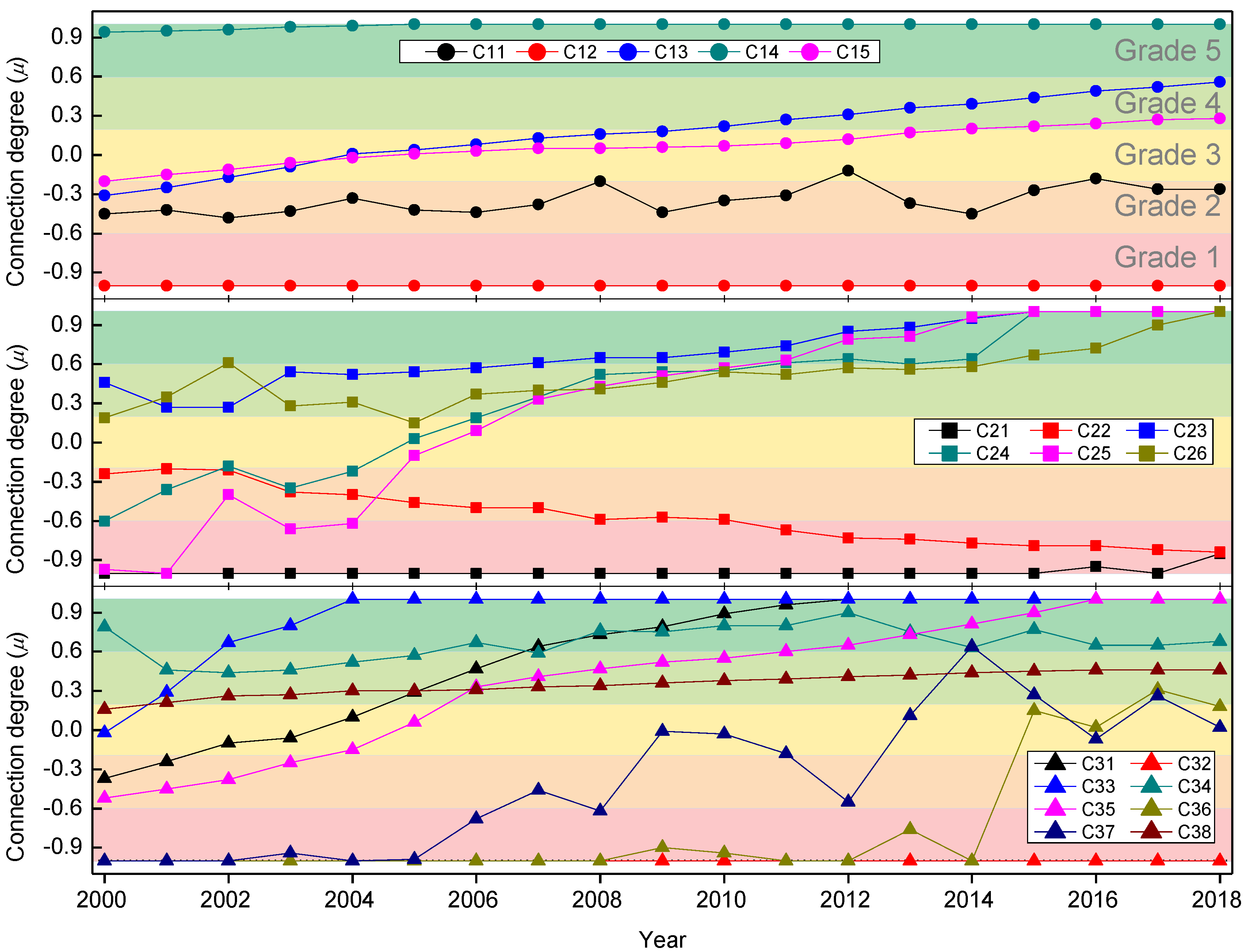
A value of −1 is set for the contradistinction degree, indicating that the indicator condition is extremely poor. According to the principle of equal division, the discrepancy degree coefficients (i₁, i₂, and i₃) are determined based on the equally dividing the interval of [−1,1]. Specifically, i₁ = 0.5, i₂ = 0, and i₃ = −0.5. The variations in the connection degrees of indicators C11–C38 and the corresponding grades are depicted in Figure 4.

The top panel of Figure 4 shows the variations in the connection degree of the indicators related to the dynamic component of the SWRS. C12 is the per capita local water resources in Beijing. The connection degree was −1 from 2000 to 2018 (red circles), belonging to grade 1, reflecting a poor performance. During this period, the per capita local water resources in Beijing varied between 90 and 165 m³/person, which is much lower than the international standard of severe water scarcity (<500 m³/person). Such a high population pressure on the water subsystem of Beijing could severely weaken the dynamics of the SWRS, negatively affect the sustainable utilization of water resources and hinder the development of socioeconomic status of the Beijing megacity. However, C14 (urbanization rate) displays an excellent performance. The urbanization rate of Beijing increased from 77.5 to 86.5%, reflecting rapid growth. The connection degree varied from 0.94 in 2000 to 1 in 2005 and remained at grade 5 during this period (dark cyan circles in Figure 4). Therefore, rapid and high-level urbanization has greatly promoted the socioeconomic development of Beijing and is very favorable to the conservation, efficient utilization, and integrated management of water resources. The black circles (Figure 4) indicate the variations in the connection degree of C11 (annual precipitation). Although the connection degree lightly increases overall, it fluctuates near grade 2, which reflects a poor situation. This result illustrates that the annual precipitation in Beijing, although relatively limited, has a stable influence on the SWRS among all the dynamic indicators. For indicators C13 (per capita GDP) and C15 (forest coverage), the connection degrees exhibit a similar trend. From 2000 to 2018, the per capita GDP of Beijing increased by a factor of nearly five, and the forest coverage increased by 50%. The connection degree of C13 varied from −0.31 in 2000 to 0.56 in 2018, and the corresponding grade increased from 2 (poor) to 4 (good). The connection degree of C15 ranged from −0.20 in 2000 to 0.28 in 2018 and the grade of this indicator changed from medium to good. Therefore, these two indicators were major factors improving the dynamic conditions of the SWRS in Beijing.

The middle panel of Figure 4 depicts the variations in the connection degree of the indicators related to the resistance component of the SWRS. Although the water resource development ratio (C21) in Beijing decreased from 204 to 54%, it is still very high. Therefore, the connection degree (black squares) is still −1, and this indicator is at a very poor level. From 2000 to 2018, the proportion of domestic water consumption (C22) in Beijing increased due to the increase in the population. As a result, the connection degree decreased from grade 2 (poor) to grade 1 (very poor). The indicators other than C21 and C22 exhibited a good performance, and their connection degrees increased significantly. The change in the connection degree of C25 was the most significant, increasing from −1 to 1. The proportion of water supplied by the eco-environment in Beijing increased from 1.1% in 2000 to 34.1% in 2018, which fundamentally reversed the impact on the SWRS (i.e., shift from resistance to a driving force). C23 (proportion of domestic water consumption) and C26 (proportion of sewage discharge) also have a positive impact on the SWRS.

The final panel in Figure 4 shows the variations in the connection degrees of the indicator related to the coordination component of the SWRS. One indicator, namely, per capita daily domestic water use (C32), displays a very poor performance. The connection degree of C32 remained at −1 and is classified as grade 1. The per capita daily domestic water use is between 205 and 260 m³/(person day), which is far higher than the standard for urban residential use in China (85–140 L/(person day) in Beijing and other cities). In the early period, the connection degree of indicators C36 and C37 was −1, reflecting the very poor performance of the SWRS in Beijing. However, with the increase in water supply provided by the South to North Project and reclaimed water, the connection degrees of these two indicators increased significantly in the later period. The connection degree for C37 was excellent in 2014 and those for C36 and C37 have been stable at medium and good levels in recent years. The proportion of agriculture in Beijing is very small, and agricultural products have accounted for less than 1% of the total GDP since 2007. Additionally, the agricultural water use efficiency in Beijing is very high at between 3000 and ~4500 m³/hm⁻². Hence, the connection degree of C34 is good to excellent (between 0.4 and 0.9). The connection degrees of other indicators (C31, C33, C35 and C38) have been increasing and had positive coordination effects on the SWRS of Beijing.

4.2. Dynamic Analysis of the Operating Mechanism of the Beijing’s SWRS

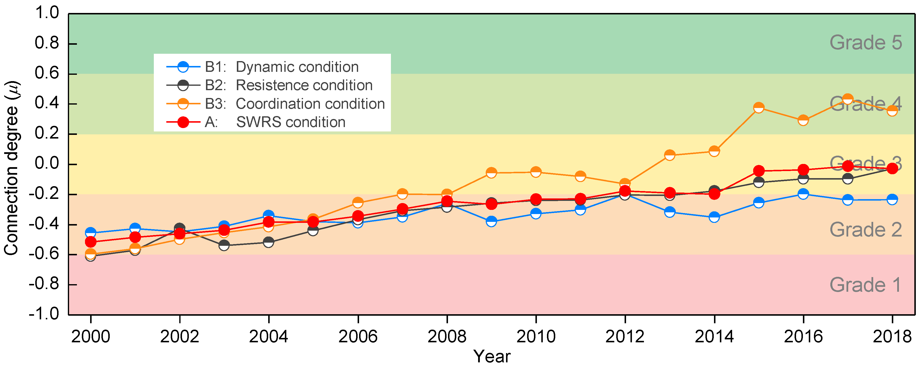
According to the steps in the AHP method, the weights of C22–C26, C31–C38 and B1–B3 can be determined. The weights of indicators in the index and criterion layers are shown in

Table 9. The indicator weights for the criterion layer and the index layer.

Criterion Layer (B)	Weight (ωm)	Index Layer (C)	Weight (ωpq)	Index Layer (C)	Weight (ωpq)	Index Layer (C)	Weight (ωpq)
B1	0.581	C11	0.510	C21	0.405	C31	0.075
B2	0.110	C12	0.229	C22	0.150	C32	0.086
B3	0.309	C13	0.055	C23	0.055	C33	0.094
		C14	0.055	C24	0.113	C34	0.045
		C15	0.152	C25	0.154	C35	0.140
				C26	0.123	C36	0.290
						C37	0.170
						C38	0.101

. Given the weights in Table 9 and the identity, discrepancy or contradistinction degrees of indicators in the index layer, the connection degrees of indicators in the criterion layer and the goal layer can be calculated using Equations (A2) and (A3), and the results are depicted in Figure 5.

As shown by the red solid dots and lines in Figure 5, the connection degree of the SWRS condition in Beijing annually increased from −0.52 in 2000 to −0.03 in 2018. However, the corresponding indicator grade only changed from grade 2 to grade 3, namely, from poor to medium. In addition, the connection degree was negative until 2018. These results illustrate that the sustainability of the Beijing SWRS is improving, but this improvement has not been very significant and the sustainability of the Beijing SWRS has not yet fundamentally changed.

The dynamic conditions (B1), resistance conditions (B2) and coordination conditions (B3) are the components of the goal layer (SWRS conditions (A)). The connection degrees of these three indicators increased overall, indicating that these indicators all have a positive influence on improving the sustainability of the Beijing SWRS. Figure 5 shows that the rates of change of the connection degrees of these three indicators were relatively consistent in the former period (2000–2008) and began to diverge after 2008, with the coordination indicator increasing fastest, the dynamic conditions indicator increasing slowest and resistance conditions indicator increasing at a medium rate. Table 9 shows that the indicator weight of the dynamic conditions indicators is 0.58, which is higher than those of the other two indictors. Therefore, the variations in the dynamic conditions mainly determine the overall trend of the SWRS conditions.

As shown by the blue half-filled dots and lines in Figure 5, the connection degree of the dynamic conditions indicator slowly increases from −0.45 to −0.23, thus remaining at the grade 2 level (i.e., poor level). This finding suggests that although the dynamic conditions of the Beijing SWRS are gradually improving, this improvement is very slow and influences variations in the SWRS conditions. For the resistance conditions indicator, the connection degree annually increased from −0.61 to −0.03, and the indicator grade rose from grade 2 to 3 (i.e., from poor to medium). Thus, the negative influence of the resistance factors on the Beijing SWRS decreased, and the positive effect increased. For the three factors that influence the operating mechanism of the SWRS, the coordination conditions indicator has the most positive effect; notably, the corresponding connection degree significantly increases from −0.60 to 0.35, and the corresponding grade rises from 2 (poor) to 4 (good). This significant change from negative to positive is fundamental to the overall improvement in sustainability. As the indicators related to the coordination mechanism have improved, the effects of the coordination mechanism on the SWRS have become increasingly important.

4.3. Discussion on the Grading Threshold of Indicators

The selection and grading of indicators are subjective in the comprehensive evaluation of water resources, environment or disasters. This subjectivity has become a controversial issue that causes the objectivity of the evaluation results and is also a question that is often asked. It is important to look at this issue from two perspectives. On the one hand, this issue is influenced by many factors and is also very complex, which poses many difficulties and challenges to understanding and the accurately quantitative evaluation. On the other hand, a comprehensive evaluation is a study that involves the interdisciplinarity of social and natural sciences. It has its unique features, and requires a novel horizon and novel thinking to answer the faced questions.

There are many factors that make the selection and grading of indicators subjective, such as different geographical regions, different ecological protective objectives, different development stages and changes in management policies, etc. The existence and influence of these factors are objective and unavoidable. For example, the focus of an indicator system in selecting indicators is different in different geographical regions for the evaluation of water resources sustainability. In regions with abundant precipitation, water quality is a major factor influencing water shortages and indicators related to water quality should be selected. However, in arid and semiarid regions, precipitation may be a critical factor causing water shortage, so indicators related to precipitation are the focus of consideration. In addition, the grading of the same indicator should be different in different regions. For example, vegetation type and coverage degree in desert and rainforest regions are significantly different according to the laws of zoning in physical geography—desert vegetation is sparse and rainforest vegetation is dense. If the indicator grading of rainforest vegetation is employed to measure the vegetation in desert regions, the evaluation result is definitely very bad, which is not realistic. Under national conditions, desert vegetation should be sparse and is very healthy, which is determined by the local hydrothermal conditions. Therefore, the grading of vegetation indicator in the two geographical regions should be different and adapted based on the local conditions. The grading of indicators should vary with different evaluation objectives for the same topic. For example, the proportion of agricultural areas in a country may vary from 5 to 30% according to different nature protection goals [45]. In addition, the allowable values of some indicators vary with different stages of socioeconomic development. For example, generally, in the early stage of economic development for a country, sewage treatment may not be the performance assess index of the local government. Environmental problems become more and more serious with economic development, and the government will demand higher and higher sewage treatment rates. In China, the urban sewage treatment rate has increased from 75.25% in 2009 to 91.90% in 2015 [46]. If the sewage treatment rate of a city is 70% in China, ten years ago it would have been evaluated as a very good environmental performance, but now it would be a very poor rating. These subjectivity (or uncertainties), caused by the regions, objectives and development stages, can be controlled or increased by constructing a causal or overall framework for the selection and grading of indicators based on some general guidelines and they can be also corrected according to practical experience.

The rationality or explanation of the grading thresholds of some indicators has been studied. For example, a 20 and 40% annual water withdrawal to availability are generally categorized as the accepted thresholds for medium and high water stress, respectively [47]. However, the rationale for these two thresholds has not been fully explained. Hanasaki et al. [48] quantitatively investigated the empirical water stress thresholds using a state-of-the-art global hydrological model and addressed two well-known questions—(1) under what hydrological conditions do conventional water scarcity indicators represent water stress; (2) are there alternative methods to set the thresholds to reflect regional variations? In addition, more and more methods, such as a socio-ecohydrological thresholds framework, spatial statistical method, geostatistics model, etc., are being employed to study or determine the grading thresholds for some evaluation indicators [49,50]. Therefore, more and more studies on the rationale of the grading thresholds of evaluation indictors will enhance the accuracy and objectivity of the evaluation results.

5. Conclusions

To explore the sustainability of water resource development in megacities, according to the definition of an SWRS, this paper analyzed the operation mechanism of an SWRS with dynamic, resistance and coordination mechanisms. A universal indicator system for SWRS evaluation was constructed based on three major operating mechanisms. This universal indicator system was divided into three layers: goal, criterion and index layers. The SWRS condition was the goal indicator. The criterion layer contained three indicators for dynamic conditions, resistance conditions and coordination conditions. The indicators of the index layer corresponding to each of the three criterion indicators are related to the water subsystem, ecological subsystem, social subsystem and economic subsystem. To solve the problem of the fuzziness of threshold values for the grading standards, a model for SWRS evaluation was constructed based on the SPA method, the AHP method and the attribute interval recognition method. This model is conceptually simple and convenient to apply. Finally, as a case study, this paper constructed an evaluation indicator system of the Beijing SWRS and evaluated the dynamics of the sustainability of this SWRS and the corresponding operating mechanism during periods beginning in 2000 and 2008. The results show that the three operating mechanisms all play a positive role improving the sustainability of water resource development in the Beijing megacity, but their variations have generally been limited, except those for the coordination conditions. Therefore, the sustainability of the Beijing SWRS can be considerably improved.

References

- WWAP, (UNESCO World Water Assessment Programme). The United Nations World Water Development Report 2020: Water and Climate Change; UNESCO: Paris, France, 2020; p. 235. Available online: https://en.unesco.org/themes/water-security/wwap/wwdr/2020 (accessed on 14 June 2020).
- AQUASTAT. FAO’s Global Information System on Water and Agriculture. Available online: http://www.fao.org/aquastat/en/overview/methodology/water-use/ (accessed on 22 June 2020).
- WWAP, (UNESCO World Water Assessment Programme). The United Nations World Water Development Report 2016: Water and Jobs; UNESCO: Paris, France, 2016; p. 164. Available online: https://www.unwater.org/publications/world-water-development-report-2016/ (accessed on 22 June 2020).
- Burek, P.; Satoh, Y.; Fischer, G.; Kahil, T.; Jimenez, L.; Scherzer, A.; Tramberend, S.; Wada, Y.; Eisner, S.; Flörke, M.; et al. Water Futures and Solution—Fast Track Initiative (Final Report); International Institute for Applied Systems Analysis (IIASA): Luxemburg, 2016; p. 113. Available online: http://pure.iiasa.ac.at/id/eprint/13008/ (accessed on 22 June 2020).
- OECD (Organization for Economic Co-Operation and Development). OECD Environmental Outlook to 2050: The Consequences of Inaction; OECD: Paris, France, 2012; p. 350. Available online: https://doi.org/10.1787/9789264122246-en (accessed on 25 June 2020).
- IEA (International Energy Agency). Excerpt from the World Energy Outlook 2016; IEA: Paris, France, 2016. Available online: https://www.iea.org/reports/world-energy-outlook-2016 (accessed on 25 June 2020).
- Brundtland, G.H. Our Common Future: Report of the World Commission on Environment and Development; Oxford University Press: Oxford, UK, 1987; p. 383. [Google Scholar]
- Hermanowicz, S.W. Sustainability in water resources management: Changes in meaning and perception. Sustain. Sci. 2008, 3, 181–188. [Google Scholar] [CrossRef] [Green Version]
- Postel, S.L.; Daily, G.C.; Ehrlich, P.R. Human Appropriation of Renewable Fresh Water. Science 1996, 271, 785–788. [Google Scholar] [CrossRef]
- Loucks, D.P. Quantifying trends in system sustainability. Hydrol. Sci. J. 1997, 42, 513–530. [Google Scholar] [CrossRef]
- Dai, D.; Sun, M.; Lv, X.; Lei, K. Evaluating water resource sustainability from the perspective of water resource carrying capacity, a case study of the Yongding River watershed in Beijing-Tianjin-Hebei region, China. Environ. Sci. Pollut. Res. 2020, 27, 21590–21603. [Google Scholar] [CrossRef] [PubMed]
- Chaturvedi, M.C.; Srivastava, D.K. Study of a complex water resources system with screening and simulation models. Water Resour. Res. 1981, 17, 783–794. [Google Scholar] [CrossRef]
- Feng, S.Y. The Water Resources System Engineering; Hubei Scienc and Technology Press: Wuhan, China, 1991. (In Chinese) [Google Scholar]
- Loucks, D.P. Sustainability Criteria for Water Resource Systems; Cambridge University Press: Cambridge, UK, 1999. [Google Scholar]
- Sandoval-Solis, S.; McKinney, D.C.; Loucks, D.P. Sustainability Index for Water Resources Planning and Management. J. Water Resour. Plan. Manag. 2011, 137, 381–390. [Google Scholar] [CrossRef] [Green Version]
- Fowler, H.J.; Kilsby, C.G.; O’Connell, P.E. Modeling the impacts of climatic change and variability on the reliability, resilience, and vulnerability of a water resource system. Water Resour. Res. 2003, 39, 39. [Google Scholar] [CrossRef] [Green Version]
- Khranovich, I.L. Stability of functioning of water resource systems. Water Resour. 2007, 34, 485–495. [Google Scholar] [CrossRef]
- Li, Y.; Lence, B.J. Estimating resilience for water resources systems. Water Resour. Res. 2007, 43, W07422. [Google Scholar] [CrossRef]
- Koop, S.H.A.; van Leeuwen, C.J. Assessment of the Sustainability of Water Resources Management: A Critical Review of the City Blueprint Approach. Water Resour. Manag. 2015, 29, 5649–5670. [Google Scholar] [CrossRef] [Green Version]
- Zhang, M.; Zhou, J.; Zhou, R. Evaluating Sustainability of Regional Water Resources Based on Improved Generalized Entropy Method. Entropy 2018, 20, 715. [Google Scholar] [CrossRef] [Green Version]
- Ghasemi, A.; Saghafian, B.; Golian, S. System dynamics approach for simulating water resources of an urban water system with emphasis on sustainability of groundwater. Environ. Earth Sci. 2017, 76, 637. [Google Scholar] [CrossRef]
- Ryu, J.H.; Contor, B.; Johnson, G.; Allen, R.; Tracy, J. System Dynamics to Sustainable Water Resources Management in the Eastern Snake Plain Aquifer Under Water Supply Uncertainty1. J. Am. Water Resour. Assoc. 2012, 48, 1204–1220. [Google Scholar] [CrossRef]
- Sun, S.; Wang, Y.; Liu, J.; Cai, H.; Wu, P.; Geng, Q.; Xu, L. Sustainability assessment of regional water resources under the DPSIR framework. J. Hydrol. 2016, 532, 140–148. [Google Scholar] [CrossRef]
- Terasaki, S.; Nagasawa, S.Y. An Evaluation of the Sustainability of the Past and Current Management of the Water Resources in the Yellow River Basin. In Proceedings of the 2011 Aasri Conference on Environmental Management and Engineering, Wuhan, China, 26–27 November 2011; pp. 12–20. [Google Scholar]
- Vieira, E.D.O.; Sandoval-Solis, S. Water resources sustainability index for a water-stressed basin in Brazil. J. Hydrol. Reg. Stud. 2018, 19, 97–109. [Google Scholar] [CrossRef]
- Xu, Z. Urban Water Resources Management in the Yellow River Basin: Perspectives of Sustainability. In Proceedings of the 2nd International Yellow River Forum on Keeping Healthy Life of the River, Vol I, Zhengzhou, China, 16–21 October 2005; pp. 253–260. [Google Scholar]
- Yan, Y.; Feng, C.; Hu, B. Sustainability assessment of water resource in Guangxi Xijiang river basin based on composite index method. In Proceedings of the 2017 3rd International Forum on Energy, Environment Science and Materials, Shenzhen, China, 25–26 November 2017; pp. 1176–1181. [Google Scholar]
- Zhou, J.; Xu, Q.; Zhang, X. Water Resources and Sustainability Assessment Based on Group AHP-PCA Method: A Case Study in the Jinsha River Basin. Water 2018, 10, 1880. [Google Scholar] [CrossRef] [Green Version]
- Li, Y.; Wei, Y.; Li, G.; Wang, W.; Bai, Z. Sustainability evaluation of water resource system in Beijing City from a synergized perspective. China Popul. Resour. Environ. 2019, 29, 71–80. (In Chinese) [Google Scholar]
- Srdjevic, Z.; Srdjevic, B. An Extension of the Sustainability Index Definition in Water Resources Planning and Management. Water Resour. Manag. 2017, 31, 1695–1712. [Google Scholar] [CrossRef]
- WWAP, (UNESCO World Water Assessment Programme). The United Nations World Water Development Report 2019: Leaving No One Behind; UNESCO: Paris, France, 2019; p. 201. Available online: https://en.unesco.org/themes/water-security/wwap/wwdr/2019 (accessed on 5 August 2020).
- UNICEF (United Nations Children’s Fund). Country Urbanization Profiles: A Review of National Health or Immunization Policies and Immunization Strategies; UNICEF: New York, NY, USA, 2017; Available online: http://www.unicef.org/health/files/Urban_profile_discussion_paper_vJune28.pdf (accessed on 5 August 2020).
- Smith, E.T. Water Resources Criteria and Indicators. Water Resour. Update 2004, 127, 59–67. [Google Scholar]
- Du, C.; Yu, J.; Zhong, H.; Wang, D. Operating mechanism and set pair analysis model of a sustainable water resources system. Front. Environ. Sci. Eng. 2015, 9, 288–297. [Google Scholar] [CrossRef]
- Wang, H. Theory and Method on Sustainable Development System of Basin; Hohai University Press: Nanjing, China, 2000. (In Chinese) [Google Scholar]
- Jun, K.S.; Chung, E.-S.; Sung, J.-Y.; Lee, K.S. Development of spatial water resources vulnerability index considering climate change impacts. Sci. Total Environ. 2011, 409, 5228–5242. [Google Scholar] [CrossRef] [PubMed]
- Zhao, K. Set Pair Analysis Method and its Preliminary Application; Zhejiang Science and Technology Press: Hangzhou, China, 2000; pp. 1–200. (In Chinese) [Google Scholar]
- Wang, W.; Jin, J.; Ding, J.; Li, Y. A new approach to water resources system assessment—Set pair analysis method. Sci. China Ser. E Technol. Sci. 2009, 52, 3017–3023. [Google Scholar] [CrossRef]
- Srdjevic, B. Linking analytic hierarchy process and social choice methods to support group decision-making in water management. Decis. Support Syst. 2007, 42, 2261–2273. [Google Scholar] [CrossRef]
- Beijing-Water-Authority. Beijing Water Resources Bulletin (2000–2018). Available online: http://swj.beijing.gov.cn/zwgk/szygb/ (accessed on 5 August 2020).
- Beijing-Water-Authority. Beijing Water Statistical Yearbook (2016–2018). Available online: http://swj.beijing.gov.cn/zwgk/swtjnj/ (accessed on 5 August 2020).
- Beijing-Municipal-Bureau-Statistics. Survey-Office-of-the-National-Bureau-of-Statistics-in-Beijing. Beijing Statistical Yearbook (2019). Available online: http://nj.tjj.beijing.gov.cn/nj/main/2019-tjnj/zk/indexch.htm (accessed on 5 August 2020).
- The Annual Precipitation Distribution in China. Available online: http://ditu.ps123.net/china/11466.html (accessed on 5 August 2020).
- World Development Indicators. Available online: http://wdi.worldbank.org/tables (accessed on 8 August 2020).
- Herrmann, S.; Dabbert, S.; Schwarz-von Raumer, H.-G. Threshold values for nature protection areas as indicators for bio-diversity—A regional evaluation of economic and ecological consequences. Agric. Ecosyst. Environ. 2003, 98, 493–506. [Google Scholar] [CrossRef]
- Group, Z.C. Development Status and Competitive Pattern of China Sewage Treatment Industry in 2016. Available online: http://www.chyxx.com/industry/201702/496142.html (accessed on 11 September 2020).
- Shiklomanov, I.A. Comprehensive Assessment of the Freshwater Resources of the World: Assessment of Water Resources and Water Availability in the World; World Meteorological Organization: Geneva, Switzerland, 1997; p. 88. [Google Scholar]
- Hanasaki, N.; Yoshikawa, S.; Pokhrel, Y.; Kanae, S. A Quantitative Investigation of the Thresholds for Two Conventional Water Scarcity Indicators Using a State-of-the-Art Global Hydrological Model With Human Activities. Water Resour. Res. 2018, 54, 8279–8294. [Google Scholar] [CrossRef] [Green Version]
- Hough, M.; Pavao-Zuckerman, M.A.; Scott, C.A. Connecting plant traits and social perceptions in riparian systems: Ecosystem services as indicators of thresholds in social-ecohydrological systems. J. Hydrol. 2018, 566, 860–871. [Google Scholar] [CrossRef]
- Buelo, C.D.; Carpenter, S.R.; Pace, M.L. A modeling analysis of spatial statistical indicators of thresholds for algal blooms. Limnol. Oceanogr. Lett. 2018, 3, 384–392. [Google Scholar] [CrossRef]
- Li, Q.; Ning, L. Attribute Interval Recognition Theoretical Model with Application. Math. Pract. Theory 2002, 32, 50–54. (In Chinese) [Google Scholar]
Figure 1.
The geographical location and administrative map of the Beijing megacity in China.
Figure 2.
Relationships among subsystems in a sustainable water resource system (SWRS) (revised from Du et al., 2015 [34]).
Figure 3.
Operating mechanisms of an SWRS and its components.
Figure 4.
Variations in the connection degrees for indicators C11–C38 and their grades.
Figure 5.
Dynamics of the connection degree of the SWRS condition and its components.