A Molecular-Level Picture of Electrospinning


1
Department of Chemistry, Faculty of Science, Jan Evangelista Purkyně University in Ústí nad Labem, Pasteurova 3632/15, 400 96 Ústí nad Labem, Czech Republic
2
Department of Membrane Separation Processes, Institute of Chemical Process Fundamentals, Czech Academy of Sciences, Rozvojová 135/2, 165 02 Praha 6, Czech Republic
3
Department of Nonwovens and Nanofibrous Materials, Faculty of Textile Engineering, Technical University of Liberec, Studentská 1402/2, 461 17 Liberec 1, Czech Republic
*
Author to whom correspondence should be addressed.
Water 2020, 12(9), 2577; https://doi.org/10.3390/w12092577
Submission received: 14 August 2020
/
Revised: 9 September 2020
/
Accepted: 12 September 2020
/
Published: 15 September 2020
(This article belongs to the Special Issue Experiments in a Floating Water Bridge and Electrified Water)
Abstract
:Electrospinning is a modern and versatile method of producing nanofibers from polymer solutions or melts by the action of strong electric fields. The complex, multiscale nature of the process hinders its theoretical understanding, especially at the molecular level. The present article aims to contribute to the fundamental picture of the process by the molecular modeling of its nanoscale analogue and complements the picture by laboratory experiments at macroscale. Special attention is given to how the process is influenced by ions. Molecular dynamics (MD) is employed to model the time evolution of a nanodroplet of aqueous poly(ethylene glycol) (PEG) solution on a solid surface in a strong electric field. Two molecular weights of PEG are used, each in 12 aqueous solutions differing by the weight fraction of the polymer and the concentration of added NaCl. Various structural and dynamic quantities are monitored in production trajectories to characterize important features of the process and the effect of ions on it. Complementary experiments are carried out with macroscopic droplets of compositions similar to those used in MD. The behavior of droplets in a strong electric field is monitored using an oscilloscopic method and high-speed camera recording. Oscilloscopic records of voltage and current are used to determine the characteristic onset times of the instability of the meniscus as the times of the first discharge. The results of simulations indicate that, at the molecular level, the process is primarily driven by polarization forces and the role of ionic charge is only minor. Ions enhance the evaporation of solvent and the transport of polymer into the jet. Experimentally measured instability onset times weakly decrease with increasing ionic concentration in solutions with low polymer content. High-speed photography coupled with oscilloscopic measurement shows that the measured instability onset corresponds to the formation of a sharp tip of the Taylor cone. Molecular-scale and macroscopic views of the process are confronted, and challenges for their reconciliation are presented as a route to a true understanding of electrospinning.
Keywords:
electrospinning; polymer solution; molecular dynamics; ions; electric field; Taylor cone; liquid jet
1. Introduction
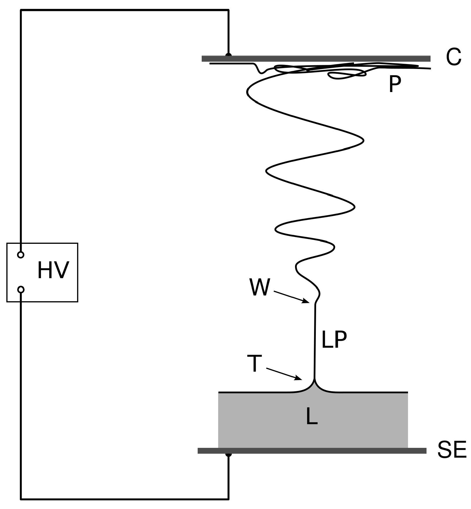
Electrospinning is a technique utilizing high-voltage (HV) electric fields to produce nanofibrous materials from polymer solutions or, less commonly, polymer melts [1]. In the electrospinning device (for a schematics see Figure 1), the strong electric field destabilizes the surface of the liquid connected to a terminal of a high-voltage power supply, and the liquid subsequently forms a pointed meniscus, the Taylor cone. A discharge in the form of a thin liquid jet then emanates from the tip of the cone. The liquid jet is not always stable and may disintegrate into liquid aerosol leading to an electrospray, which is itself an important phenomenon in applied physics [2,3]. When the jet arrives at the counter-electrode, a collector, it deposits as a solid nanofiber. In the case of solution spinning (which is the most common one), solidification is facilitated by rapid evaporation of the solvent. Bending, or whipping, instability occurring after a short linear path of the jet significantly contributes to elongation and thinning of the jet [4,5]. By depositing many layers of nanofibers, a non-woven fabric is created on the collector showing exceptional porosity and surface-area-to-volume ratio [6]. Owing to their unique properties and versatility of their preparation, electrospun nanofabrics find a wide variety of applications, such as air filtration [7,8], oil/water separation [9], drug delivery [10,11], or tissue engineering [12]. With the outbreak of the novel coronavirus pandemic (COVID-19) in 2020, electrospun materials have gained attention as a promising active layer for protective face masks [13].
The theoretical description of electrospinning and related phenomena has predominantly relied on electrohydrodynamic models formulated within continuum mechanics [5,15,16]. The fundamentals of theoretical understanding of the field-induced phenomena at liquid interfaces related to electrospray and electrospinning were laid by Lord Rayleigh [17], John Zeleny [18], and most notably sir Geoffrey Ingram Taylor [19,20,21], who studied a conical formation occurring on liquid surfaces in strong electric fields, the formation which today bears his name: the Taylor cone. Conventional electrohydrodynamic approach to weakly conducting fluids in electric fields, the Taylor–Melcher leaky dielectric model [16], incorporates both dielectric polarization and ionic conduction in terms of the Maxwell stress tensor and conservation equations. If the charge relaxation time, , is much lower than the hydrodynamic relaxation time, , the behavior of a leaky dielectric liquid approaches that of a perfect conductor, and when the opposite is true, i.e., , the liquid behaves as an insulator. The former situation is assumed to take place when the Taylor cone builds, whereas the latter is believed to exist in a flying jet [5]. For a modern review on continuum modeling of electrospinning, we refer the reader to the monograph of Ko and Wan [22] or the chapter by Rafiei [23].
Apart from the conventional continuum modeling one can also find reports on methods involving discrete macro- or mesoscopic elements. The entire jet can be modeled as a chain of charged particles connected by visco-elastic links with one another as, e.g., in works of Reneker et al. [4] or Lauricella et al. [24,25]. Mesoscopic modeling incorporating individual polymer chains was performed by Liu et al. [26,27,28,29], who employed the dissipative particle dynamics to model polymer melt electrospinning using a coarse-grained model of chains. The dissipative particle dynamics was also applied by Joulaian et al. [30] to model the initial stages of the formation of the Taylor cone.
Truly atomistic simulations of electrospinning with explicit solvent are scarce in the literature. Jirsák et al. published several works [31,32,33,34,35] developing and applying an approach to model electrospinning by atomistic molecular simulations in several geometries of the simulation cell using the rigid water model, simple sodium chloride ions and model poly(ethylene glycol) (PEG) chains. Jirsák et al. concluded that even a perfect dielectric (model water) was able to jet in electric field and revealed a link between liquid jetting and bridging. In a similar, independent study, Wang et al. [36] investigated the behavior of a polymer solution droplet in the electric field and the influence of ions on spinnability.
The above-mentioned previous works [31,32,33,34,35] co-authored by the first author represent a continuing effort to tackle the atomistic modeling of electrospinning methodologically and to understand the process on a fundamental, molecular level. In the first article [31], Jirsák et al. partitioned the process of electrospinning into zones accessible to modeling (free liquid surface, the tip of the Taylor cone, and the linear segment of the liquid jet) and proposed several strategies for implementation of molecular simulation in the respective zones. Application of the developed methodology to pure water and aqueous sodium chloride revealed that at atomic scale ions play only a marginal role in jet initiation; nevertheless, their presence destabilizes the jet. In the subsequent paper [32], the authors noticed an interesting analogy between the liquid jet in electrospinning and a cylindrical structure created by water in electric field, the ‘floating water bridge’ [37]. In paper [33], the authors further investigated the influence of ions on the stability of field-induced liquid cylinders, monitored the mass flow in jets and added a model of polymer to the system (PEG). In Ref. [34], Jirsák et al. analyzed polymer conformation and solvation during jetting. They concluded that polymer chains unfolded when entering the jet and that they remained well solvated despite progressing fragmentation of the solvent. The invited chapter [35] presented an comprehensive overview of the developed methodology and summarized the achieved results.
In the present contribution, the authors work further towards understanding the molecular mechanism of electrospinning, especially its initial stages: formation of the Taylor cone and the onset of jetting. Following the methodology developed earlier [31,32,33,34,35], systematic simulations of saline aqueous solutions of PEG are performed and analyzed with respect to a wide range of dynamic and structural properties. Unlike the previous studies, the present work adds laboratory experiments performed on the solutions of composition comparable to that used in simulations. An oscilloscopic method developed by P. Pokorný and coworkers at the Technical University of Liberec [38,39] is used to measure the latency time before the first Taylor cone builds and discharges.
The remaining part of the article is organized as follows. In the next section, methods utilized in molecular simulations and experiments are described along with all parameters necessary for reproduction. The following section, Results and Discussion, compiles the data produced by simulations and experiments, offers the interpretation of the data, and finally discusses how molecular and macroscopic observations might be related. Limitations of the present study are also discussed. The last section, Conclusions, summarizes main findings of the work and outlines challenges for future research.
2. Methods
2.1. Computational
2.1.1. Molecular Simulations
Classical molecular dynamics simulations of a nanodroplet of polymer solution on a solid underlay in strong electric fields were performed. GROMACS 4 package [40,41] was employed for all simulations, using the GROMOS 53A6 force field [42] with simple point-charge (SPC) water model [43]. The leap-frog integrator with time step 2 fs was used. Bond lengths in polymer chains were constrained by P-LINCS [44] algorithm, SETTLE [45] was used to constrain a rigid water geometry.
The simulated polymer solutions comprised of three components: water, sodium chloride, and hydroxyl-terminated poly(ethylene glycol). Two different numbers of –O–CH–CH– monomer units, 119 and 239, were used, corresponding to PEG molecular weights 5260 Da and 10,547 Da, respectively. The number of water molecules in all solutions was around 23,700, whereas the population of other components varied. For sodium chloride, , 18, 36, or 72 of Na Cl ion pairs were used. For 5260-Da polymer, , 12, or 16 chains were used, while for 10,547-Da polymer, , 6, or 8 chains were used. Initial configurations were prepared in a cubic cell using the highest concentrations of ions and polymer. The cube of the solution was then left to adhere to the surface of an underlay during a pre-equilibration stage until it formed a hemispherical droplet. Samples with lower concentrations were built by deleting excess solute molecules from the initial droplet of concentrated solution. The initial configurations resulting from the pre-equilibration step were then used for equilibration described later.
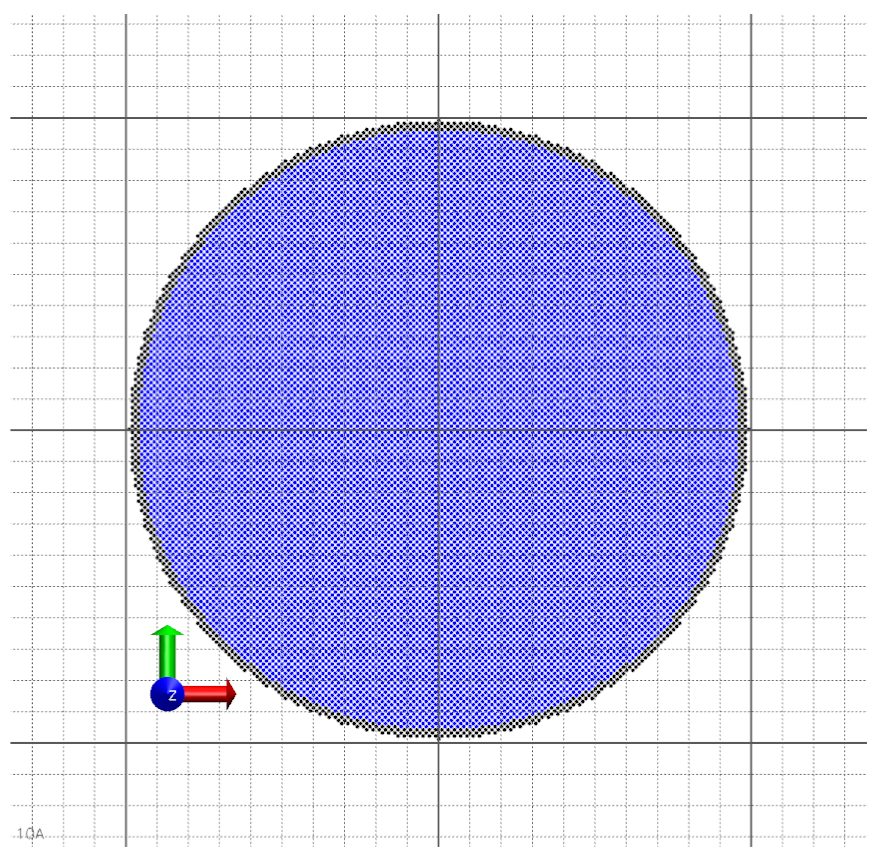
The support of a droplet was formed by a planar disc, ca. 20 nm in diameter, made of 15,384 Lennard-Jones (LJ) sites with positions fixed onto a square grid at with spacing 0.14142 nm. The LJ parameters of the underlay sites, kJ mol nm and kJ mol nm, were adjusted to maintain a reasonable contact angle of the droplet close to 90. Geometric combination rules were applied for cross-interactions of the underlay with other components. In order to prevent accidental ‘spilling’ of the liquid over the rim to the other side of the disc, the parameters of 912 sites of the rim (two outermost circles) of the underlay were modified to render a purely repulsive interaction by zeroing , keeping unchanged. See Figure 2 for a graphical representation of the underlay. Figure 3 shows the underlay with a droplet.
A typical simulation protocol involved (i) a long 10-ns equilibration under periodic boundary conditions (PBC) in all directions at constant temperature K maintained by the Berendsen thermostat [47] with time constant ps, (ii) a short 1-ns equilibration without PBC using the stochastic velocity-rescaling thermostat of Bussi et al. [48] with the same T and , and finally (iii) a non-thermostated production run without PBC under a stationary and uniform electric field applied in the normal direction to the underlay plane (positive z-axis). The production run lasted tens to hundreds of picoseconds. Between stages (i) and (ii), water molecules with oxygens located farther than 10 nm from the center of the disc were deleted to limit the number of molecules initially present in vapor phase.
In simulations with PBC, a cubic simulation box with edge length 25 nm was used. Electrostatic forces in an infinite periodic system were treated by the particle-mesh Ewald method [49] with cut-off 2 nm, grid spacing 0.3 nm, cubic interpolation, and the relative strength of the direct potential at cut-off [41]. Lennard-Jones forces were neglected beyond a cut-off distance of 1.5 nm. In production runs without PBC, all site–site interactions were included in the calculation of the force, i.e., there was no potential cut-off applied.
Most of the production simulations were done with the external field intensity of 1.5 V/nm, but the effect of the strength of the field was also studied, using a series of simulation under 1.0, 1.5, 2.0, and 2.5 V/nm for selected systems. For each composition and field strength used, a single production trajectory was generated.
The national network of computer clusters Metacentrum [50] was used for all simulations, and typical computation on 32 CPU cores (AMD Opteron 6274 at 2.5 GHz) took over 11 days to equilibrate the system and another 14 hours to generate 100 ps of production trajectory.
2.1.2. Analysis of Trajectories
During the production runs, configurations of all sites were stored after each 1000 integration steps, i.e., every 2 ps, for subsequent analysis. Precision of the saved configurations was nm. For selected systems also velocities were stored to determine the kinetic energy of ions.
The cumulative net mass transfer through a plane at nm was calculated as the total mass of atoms with nm by the given time instant minus the mass of atoms with nm at the start of production (to correct for the offset caused by initially present water vapor). The time of the jetting onset was determined as the time when the cumulative mass transfer through nm overcame the threshold of 2000 Da. The mass transfer through nm of PEG chains alone was also calculated and for the corresponding onset time the threshold of 500 Da was used.
The z-position of the center of mass of all PEG chains, , was numerically differentiated with respect to time to estimate the z-component of the velocity, , of the center of mass of PEG at time instant t, i.e.,
where ps is the trajectory sampling timestep.
The evolution of the dipole moment of the whole system was calculated during production run. Two components of the dipole moment were monitored: (i) the ‘dielectric’ dipole moment of water and PEG and (ii) the ‘ionic’ dipole moment arising from sodium cations and chloride anions.
The evaporation rate of water solvent was estimated based on counting one-particle water clusters at different time instants along the trajectory. Simple criterion of oxygen–oxygen distance less than 0.35 nm was used to define a cluster bond between particles. Water molecules not having any other water molecules bound to them by a cluster bond were considered to be a part of the vapor phase. The average evaporation rate in a given time interval was determined as the change of the number of vapor molecules divided by the length of the time interval. For all samples, three evaporation rates were systematically monitored: the average rate in the first 36 ps of production, the average rate in the second 36 ps of production, and the average rate in the first 72 ps of production (i.e., a mean value of the two preceding 36-ps rates).
In order to characterize the effect of ions on the evaporation of solvent, an attempt was made to evaluate the amount of energy dissipated from the ions (accelerated by the field) to the rest of the system. The dissipated ionic energy, , was defined as the loss of the energy of ions between two chosen time instants :
The total ionic energy includes the kinetic energy of ions and the potential energy of both ion–field and ion–ion interactions:
where is the mass of the i-th ion, its velocity, its charge, and its position vector. For electrostatic potential it holds . Therefore, with we have
where the term arising from the constant vanishes in Equation (3) due to electroneutrality.
2.2. Experimental
2.2.1. Materials and Solution Preparation
The following chemicals were used for the preparation of solutions:
- Ultrapure water (18.2 M cm) was prepared by Purelab Flex 2 system (Veolia Water Systems, Ltd., High Wycombe, UK).
- Poly(ethylene glycol), = 6000 Da, was purchased from Sigma-Aldrich (Prague, Czech Republic).
- Sodium chloride p. a. was purchased from Penta (Prague, Czech Republic).
A total of 12 solutions were prepared using several different concentrations of PEG and NaCl in water. All solutions were based on ca. 100 g of water. The 12 solutions resulted from the combination of three different amounts of added PEG: 9.9, 14.8, and 19.7 g (denoted as a, b, and c PEG series, respectively), and four different amounts of added NaCl: 0.00, 0.25, 0.49, and 0.99 g (0, 1, 2, and 3 NaCl series). The above masses are only approximate, actual masses were determined to four or five significant digits for each solution. For the precise concentrations of PEG and NaCl in the prepared solutions, see Results and Discussion. Conductivities of all prepared solutions were measured by a conductivity meter (COND 51+ with 2301T cell, XS Instruments, Carpi, MO, Italy).
2.2.2. Instrumentation
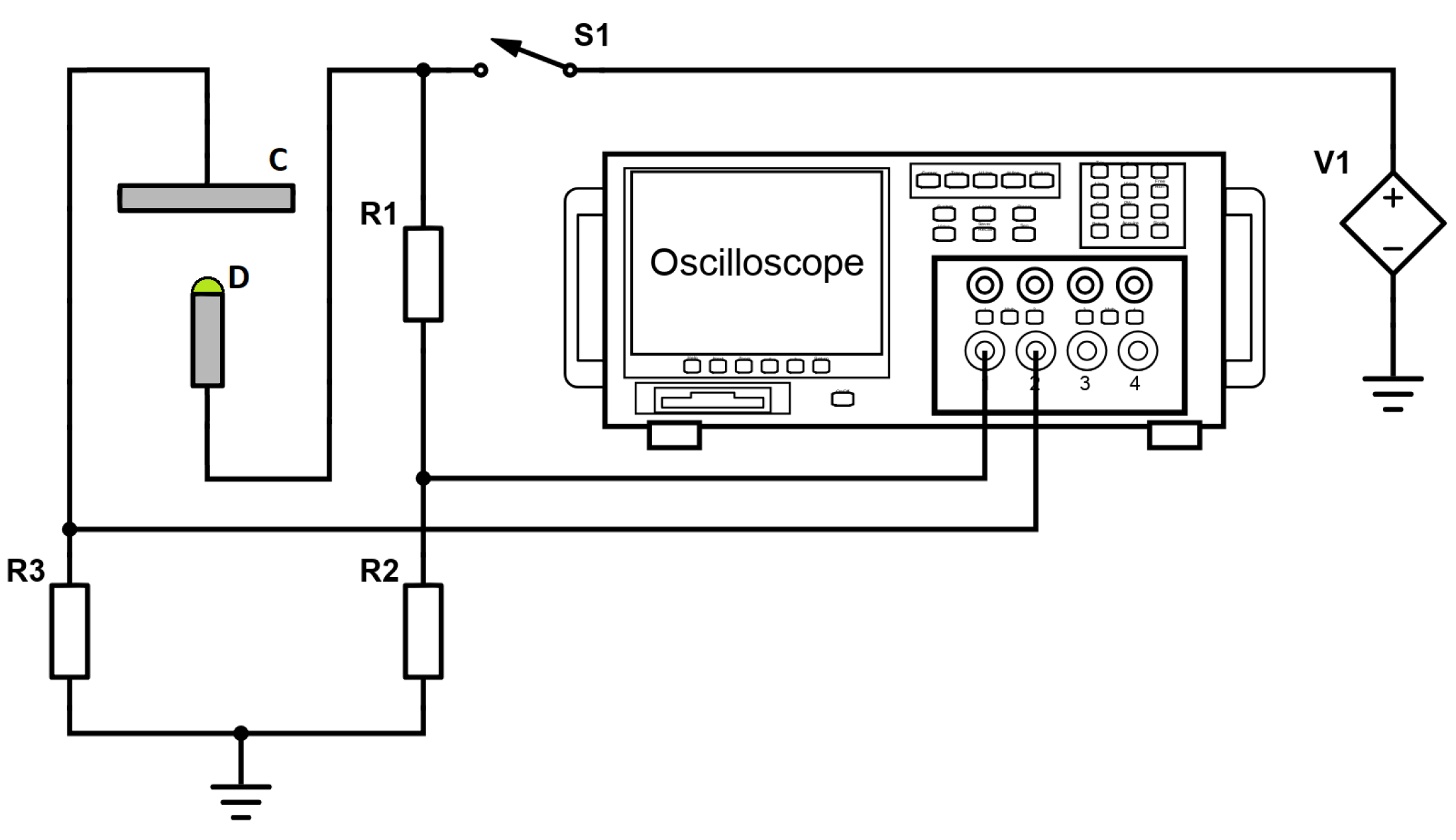
In order to monitor the instability onset, a circuit was built as shown on Figure 4. A steel working electrode was connected, through a fast-acting mechanical switch, to the positive terminal of a high-voltage direct-current power supply (AU-60P0.5-L, Matsusada Precision, Inc., Kusatsu, Japan), while the ground terminal of the supply was connected to a plate-like collector electrode. A digital oscilloscope (DS1102CD, RIGOL Technologies, Inc., Munich, Germany) was used to monitor voltage and current through the electrodes. Working electrode with a droplet was recorded by a high-speed camera (i-SPEED 720, Olympus Europa SE & Co. KG, Hamburg, Germany) with framerate 20,000 fps. For high-speed camera recording, the working electrode was illuminated by a light source (ILP-1, Olympus Europa SE & Co. KG, Hamburg, Germany) with color temperature 8200 K. The wiring of the oscilloscope to the circuit, see Figure 4, allowed for monitoring electrode voltage on channel 1 (through R1–R2 voltage divider) and electrode current directly proportional to voltage on channel 2. The delay of the rise of the current signal behind the rise of the voltage signal (at closing the switch) was considered the time of the first discharge marking the onset of the instability of the meniscus.
Two slightly different experimental setups I and II, were used, see Table 1. Setup I was used for both voltage–current delay measurement and high-speed camera recording, whereas setup II was used only for the high-speed camera recording. Figure 5 shows droplets placed on working electrodes in both setups. The high-speed camera was coupled with multifunction IO device (USB-6216-BNC, National Instruments, Austin, TX, USA) with two analog inputs (AI0 and AI1) connected to the same points as the channels of the oscilloscope in order to acquire voltage and current data synchronized with camera recording (5 data samples per frame).
Experiments were conducted according to the following protocol:
- The working electrode was briefly connected to the ground terminal to neutralize any residual charge.
- A droplet of polymer solution was placed onto the working electrode by a pipette.
- With switch S1 open, the HV power supply connected to the circuit was turned on.
- Switch S1 was closed, voltage and current signals were recorded by the oscilloscope. The behavior of the droplet was captured by the high-speed camera.
- HV supply was turned off. The working electrode was again discharged with a grounded wire.
In the case of voltage–current delay measurement, all experiments were repeated a minimum of 10 times. The droplet was placed so that it covered the whole upper surface of the rod electrode. The experiments where the droplet spilled over the edge before or during measurement were discarded. After each measurement, the electrode was carefully cleaned of the solution before placing a new droplet. Solutions with lower concentrations of ions were always placed prior to the more concentrated ones to minimize the influence of ions left adsorbed on the electrode surface.
2.2.3. Analysis of Data
Oscilloscopic records were analyzed directly in the oscilloscope. The time difference between the crests of the rising edges of voltage (channel 1) and current (channel 2) signals was considered to be the time of the instability onset, see Figure 6. High-speed camera recordings were processed by i-SPEED Software Suite (Olympus) [52].
3. Results and Discussion
3.1. Computational
3.1.1. Composition of Systems
Compositions of all systems used for MD simulations are summarized in Table 2, Table 3 and Table 4. The number of water molecules, Table 2, was around 23,700, slightly varying between samples, mainly due to vapor deletion after the first equilibration phase. Concentrations of PEG, expressed as weight fractions, are given in Table 3. Finally, Table 4 lists molalities of sodium chloride, expressed as the number of moles of NaCl per 1 kg of water. Polymer concentrations were chosen in from the range where poly(ethylene oxide) of higher molecular weights (hundreds of kDa) spins [53,54], but correspondingly long chains could not be conveniently modeled by atomistic simulation. Thus, much lower molecular weight PEG was used, such as in our previous studies [33,34,35].
3.1.2. Visual Observation
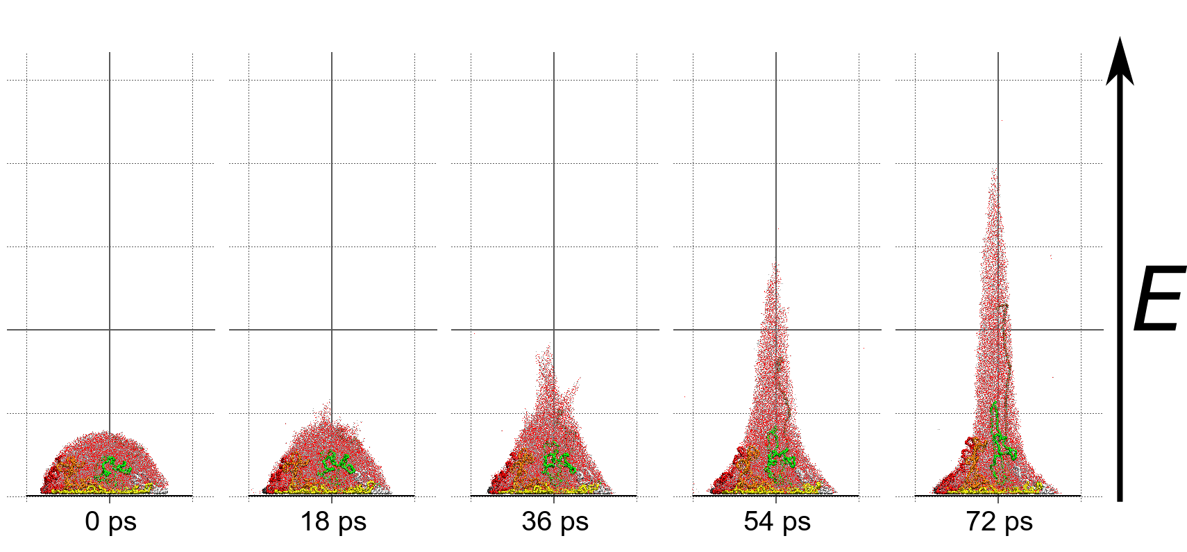
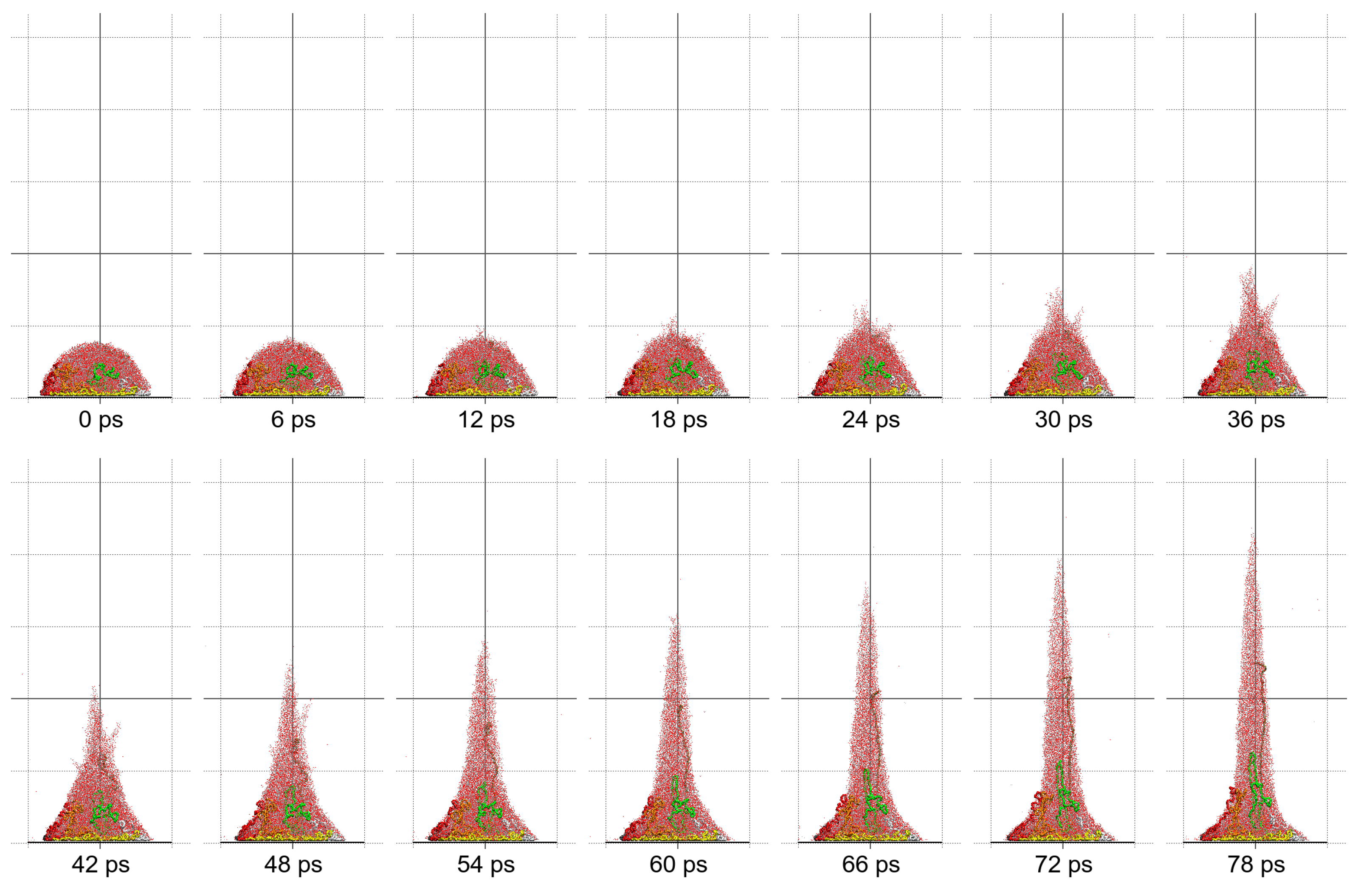
Molecular dynamics simulations performed in the present study showed the key features of the electrospinning onset, namely the Taylor cone formation and jetting. The time evolution of the simulated systems under the field of 1.5 V/nm is illustrated by the sequence of sample frames along MD trajectories of two selected systems with eight 10.55-kDa chains: one without ions, see Figure 7, and the other with 72 NaCl ion pairs, see Figure 8. Both sequences show gradual deformation of the initially spherical droplet surface, progressing to the formation of the Taylor cone at ca. 30 ps followed by ejection of mass from the cone’s tip. Before a single, well-formed jet appears, several ‘tentacles’ of solvent molecules randomly protrude from the disrupted surface.
There are some notable differences between the systems with and without ions. At first glance, samples without ions appear to be more compact, while ions seem to increase surface roughness and to enhance the fragmentation of the liquid as the process advances. Sodium cations often enter the tentacles of the solvent described in the previous paragraph and cause them to break, escaping the droplet together with a number of water molecules around them. Figure 9 shows the comparison of a system without ions and a system with ions at the same time instant—escaping sodium ions accompanied by a number of solvent molecules are clearly visible. Another interesting observation can be made concerning the interaction of ions with PEG chains. It seems ions assist the unfolding of the chains and their transport to the jet. This might be caused by the coordination of PEG ether oxygens to Na ions which are dragged by the electric field, as suggested by Wang et al. [36].
3.1.3. Transfer of Mass and Jetting Onset Times
The total net mass transport in the direction of the field through the plane at nm by the given time instant in the production runs with the applied field strength of 1.5 V/nm is plotted in Figure 10 and Figure 11 for 5.26-kDa and 10.55-kDa chains, respectively. Figure 12 shows the mass transport of the system with eight 5.26-kDa PEG chains and different number of ions for different field strengths. Figure 13 and Figure 14 show the mass transport of PEG chains alone for systems with 5.26-kDa and 10.55-kDa PEG, respectively.
The onset of jetting was characterized by the production time at which mass transfer exceeded a certain threshold. Table 5 and Figure 15 show the times when total mass transported through nm exceeded 2000 Da, whereas Table 6 and Figure 16 show the times when mass of PEG alone transported through nm exceeded 500 Da The dependence of the times when total mass transfer exceeded 2000 Da on the intensity of the field is shown in Table 7 and Figure 17 for the system with eight 5.26-kDa chains and different numbers of NaCl ion pairs.
An interesting observation is that the presence of ions had no significant impact on the total mass transfer and the corresponding onset times, while in most cases there was a discernible pattern of ions facilitating the transport of PEG chains alone, in accord with the visual observations presented above and the conclusion of Wang et al. [36]. This finding is further corroborated by Figure 18 and Figure 19 showing the velocity of PEG’s center of mass in the direction of the field, determined as a numerical derivative of the z-coordinate of the center of mass, see Equation (1). The accelerating effect of ions on PEG chains is clearly discernible, especially in the case of 10.55-kDa chains. As regards the effect of the electric field strength (Figure 17), the increase of mass transport and decrease of the corresponding onset times is not surprising and in agreement with findings at the macroscale [58].
3.1.4. Evolution of the Dipole Moment
Dielectric and ionic components of the total dipole moment under the field of 1.5 V/nm are plotted as functions of time in Figure 20 for 5.26-kDa PEG and Figure 21 for 10.55-kDa PEG. Curves for different field intensities are plotted in Figure 22 for selected systems. One can see that in all cases, dielectric polarization increased very steeply within the first 2 ps and then further moderately increased in contrast with ionic polarization, which is negligible in the beginning but takes off steeply in later stages of the process. The evolution of the dielectric dipole moment can be explained by fast dielectric saturation of molecules in the spherical droplet followed by further increase as the droplet deforms by polarization forces. The results on the dipole moment reinforce the findings that ions have little effect on mass transfer. It seems that at the molecular scale, ions play almost no role in the formation of the Taylor cone and the onset of jetting. In ion-containing systems, the same fundamental mechanisms apply as in systems with no ions at all, pointing to the clearly dielectric nature of the molecular-scale electrospinning onset.
3.1.5. Evaporation of Solvent
The rate of evaporation of solvent determined as an increase of the number of one-molecule water clusters through a chosen time period was evaluated for the periods 0–36 ps, 36–72 ps, and 0–72 ps of production time. Figure 23 shows the results for all 24 systems under 1.5 V/nm. The time 36 ps roughly corresponds to the instant when the Taylor cone has already fully developed and jetting starts under 1.5 V/nm, see Figure 7 and Figure 8. One can see that in the jetting phase (36–72 ps) and overall (0–72 ps) most simulations show the highest evaporation rate for the highest ionic concentration, but the trend is not always monotonous. Similarly to Wang et al. [36], the present authors suspect that the transfer of the kinetic energy from field-accelerated ions to the solvent is the main mechanism how the electrolyte contributes to the evaporation. In order to verify this assumption, the energy dissipated from ions was calculated for the given time periods and correlated with the evaporation rates, see bellow.
3.1.6. Energy Dissipation
The ionic energy dissipated from the beginning of production, , see Equation (2), as a function of time t, is shown in Figure 24 for selected systems, for which velocities along the trajectory were stored to allow for the evaluation of the kinetic energy.
In order to reveal a possible link between evaporation and energy dissipation, the evaporation rates in 0–36 ps, 36–72 ps, and 0–72 ps of production time were plotted against the energies dissipated through the same intervals, see Figure 25 and Figure 26. Linear regression was made and Pearson’s correlation coefficients, r, between the dissipated energy and the evaporation rate in the respective time intervals were also determined, separately for 5.26-kDa and 10.55-kDa PEG. For 5.26-kDa PEG, correlation coefficients were −0.3399, 0.9210, and 0.9125 for 0–36 ps, 36–72 ps, and 0–72 ps, respectively. For 10.55-kDa PEG, correlation coefficients were 0.3058, 0.7294, and 0.7307 for 0–36 ps, 36–72 ps, and 0–72 ps, respectively. The values of r in jetting phase and overall point to a clear correlation between the dissipated energy and the evaporation rate. Moreover, in all series of samples with the same number and length of PEG chains (same symbols in Figure 25 and Figure 26), there is always a non-decreasing trend in jetting phase and overall, unlike in the case of the dependency of the evaporation rate on the number of ion pairs, Figure 23.
3.2. Experimental
3.2.1. Preparation of Solutions
A total of 12 solutions were prepared using ultrapure water, PEG with number-average molecular weight 6000 Da, and NaCl. The composition of all solutions is summarized in Table 8 and Table 9 and roughly corresponds to the composition of solutions used in molecular simulations, see the previous subsection. Table 10 lists the measured conductivities of the solutions.
3.2.2. Oscilloscopic Measurements
Table 11 and Figure 27 summarize the results of voltage–current delay measurements used to characterize the onset of the instability of the meniscus. The measurements were done using setup I (see Table 1) at air temperature 24.0 C and relative humidity 60%. PEG series a and b show a weak tendency of the onset time to decrease with increasing ionic concentration, whereas the solutions with highest polymer concentration, PEG series c, do not show any trend.
Experimental onset times determined in this work show much weaker dependence on ionic concentration than expected for a process driven by the free charge density. For comparison, Yalcinkaya et al. [59,60] observed striking dependence of jet launching times on ionic concentration in needleless electrospinning of polyurethane and poly(ethylene oxide) solutions. Nevertheless, it should be pointed out that the instant of the first discharge measured in this work is not the same as the instant where jetting sets in. In order to elucidate what phenomena take place at the electrode, a high-speed camera coupled with oscilloscope was used.
3.2.3. High-Speed Photography
The progress of droplet deformation in setup I was recorded by a high-speed camera to complement the oscilloscopic data with visual image. Figure 28a shows the electrode current as a function of time for sample b0. The detail of the current onset phase is inserted. Figure 28b shows four photographs captured at the times marked in the detailed plot by vertical lines. Photographs show a well formed cone with an initially blunt apex, which sharpens when the first current peak is observed. No jet was visible during the onset phase, which could be caused by either the jet being too tiny to be captured in this setup or, more probably, by the absence of the jet. In the latter case, the authors believe that only the corona discharge [2] from a sharp tip of the Taylor cone was responsible for the current signal, but more data are needed to confirm this scenario. A visible jet was captured in later stages of the process with sample a0, see Figure 29. One can clearly see the ejection of a thin liquid jet from the tip of the Taylor cone and its eventual decay into visible droplets. From the time axis of Figure 29, one can get an idea how the launching of jets is delayed with respect to the first discharge, which occurred at ca. 35 ms for this particular measurement. The lateral position of the cone and the jet is caused by inhomogeneous electric field, which strengthens near the edge of the electrode.
In setup II, with the small-diameter electrode positioned horizontally, the first discharge was always accompanied by the detachment of a large portion of liquid in the form of a ‘spindle’ and large droplets. See Figure 30 for an example of the spindle observed with solution a0. Jetting was more prevalent than in setup I. A thin jet is also observable in Figure 30 at the tip of the spindle. Figure 31 and Figure 32 show cone-jet formations in later stages of the process. In Figure 31 the jet eventually transforms into visible droplets, whereas in Figure 32 no droplets are apparent. Noticeable splaying of the jet in Figure 32 might be caused by whipping instability prior to disintegration to aerosol.
3.3. Remarks on Scales
There seems to be a fundamental difference between macroscopic theories of electrospinning and the atomistic picture presented in this work. It is well established in macroscopic continuum models that electrospinning, especially in the Taylor cone formation stage, is governed by mobile (ionic) charges, and that even the fluids with the slightest concentrations of ions, unavoidable in any liquid, can be considered conducting in this regard [5]. A hypothetical pure dielectric fluid is also predicted to form a conical meniscus but not able to jet, though [61]. The above macroscopic findings seem to be in contradiction to what is observed in atomistic modeling, where ions play minor role and do not significantly affect the nature of the field-induced transformation of a dielectric liquid. An interesting analogy is offered by experiments with ferrofluids, which do jet in magnetic fields [62]. Ferrofluids can be viewed as purely dipolar in principle due to nonexistence of magnetic monopoles.
The above discussed disparity deserves some explanation. First we have to realize that in simulations we work at time scales many orders of magnitude smaller than in experiments. Simulation times in tens of picoseconds put the considerations on charge relaxation to completely different perspective. The length scales are also completely different from regular electrospinning. Ions do not have enough time to create a charged interface and much possibly enough space to rise proper capillary waves against surface tension. That might shift the jetting process to the one governed by polarization forces. Hartman et al. [63] calculated with their model that although the surface charge of jetting liquid predominantly comprised the free charge in most parts of the surface of the cone and the jet, the ratio of polarization charge sharply increased at the point of the cone–jet junction, suggesting at least some role of polarization forces in this region. This lends support to the interpretation of the content of the simulation cell as a very apex of the Taylor cone where the jet starts, in accord with the simulation methodology proposed by Jirsák et al. [31] and followed herein. Contracted time and length scales are also coupled with much higher electric fields needed to observe the process. The intensities of electric fields used in simulations of electrospinning and other related phenomena are usually much higher than the average values attainable in experiments [31]. We note in passing that there are reports on related phenomena which approach the typical size of the simulation, e.g., the water bridge between an AFM tip and a sample [64].
3.4. Limitations of the Study
The present study has several limitations that should be understood for correct interpretation of the results. Some results of MD simulations lack statistical power due to limited number of simulated trajectories. The authors preferred using computing resources to cover a broader concentration range rather than to obtain several independent runs for a limited number of systems. Only nonpolarizable models were used for all components, which could affect dynamic properties. It is known that nonpolarizable models of ions and water do not correctly reproduce water diffusivity in electrolyte solutions [65]. Similarly to all molecular simulation studies in electric fields, it is not clear how to exactly relate the field applied in simulation to the macroscopic one.
As regards laboratory experiments, it should be pointed out that they play only a complementary role in the present study and were mainly motivated by authors’ curiosity to learn how the solutions used in simulations would present themselves at macroscale. The solutions were expected to spray rather then spin, which showed to be the case. The most important information the authors wanted to extract from the experiments was the dependence of the characteristic time of the Taylor cone build-up on composition. In future studies, a search should be made for the set of conditions where jetting in simulations is more closely related to real fiber-producing experiments. The technique of measurements could also be improved. In the present study, the volume of droplets and their exact position with respect to the edge of the electrode were not precisely controlled for, which introduced additional scatter to the measured onset times, as the field intensity varies very steeply near the edges.
4. Conclusions
Molecular dynamics simulations of a nanosized droplet of polymer solution subjected to strong electric fields were performed. Formation of the Taylor cone and subsequent jetting accompanied by rapid evaporation of solvent was observed. The results indicate that at molecular scale, the formation of the cone and the onset of jetting is governed by dielectric forces, in apparent contrast with macroscopic continuum models. Ions do not significantly affected the nature of the process but facilitated the transport of polymer chains into the jet and enhanced the evaporation of solvent.
Experiments were performed with similar composition of solutions as in the simulations. A weaker-than-expected effect of ions on the time of formation of the Taylor cone was found—onset times slightly decreased with increasing ionic concentration, with the exception of the highest polymer concentration where no trend was discernible. High-speed photographs show that the solution did not actually spin, which was expected. The observations are consistent with electrospray in different modes (corona discharge, cone–jet, spindle). There is not enough data to assess the effect of ions on the morphology of the process.
Apparent discord between governing mechanisms, i.e., conductive in macroscale models vs. dielectric in molecular models might be upsetting, but creates an opportunity to grasp better understanding of the underlying physics in its full complexity. Simple considerations on the time and length scales involved in experiments and in simulations might bring a relief that there is nothing fundamentally wrong with either, but only after attempting to bridge the vast space between nano- and macroscale we may truly learn something new. That is the path the present authors strive to follow in future research.
Author Contributions
Conceptualization, J.J. and P.P.; Formal analysis, J.J. and P.P.; Funding acquisition, J.J.; Investigation, J.J., P.P. and P.H.; Methodology, J.J. and P.P.; Project administration, J.J.; Resources, J.J. and P.P.; Software, J.J.; Supervision, J.J.; Validation, J.J. and P.P.; Visualization, J.J., P.H. and Š.D.; Writing—original draft, J.J.; Writing—review & editing, J.J., P.H. and Š.D. All authors have read and agreed to the published version of the manuscript.
Funding
This research was funded by the Jan Evangelista Purkyně University in Ústí nad Labem within the Student Grant Competition under Project No. UJEP-SGS-2019-53-003-2. Computational resources were supplied by the project “e-Infrastruktura C” (e-INFRA LM2018140) provided within the program Projects of Large Research, Development and Innovations Infrastructures.
Acknowledgments
Authors thank Martin Bílek, Petr Žabka, and Martin Konečný (Department of Textile Machine Design, Faculty of Mechanical Engineering, Technical University of Liberec) for providing and operating the high-speed camera.
Conflicts of Interest
The authors declare no conflict of interest. The funders had no role in the design of the study; in the collection, analyses, or interpretation of data; in the writing of the manuscript, or in the decision to publish the results.
References
- Ding, B.; Wang, X.; Yu, J. (Eds.) Electrospinning: Nanofabrication and Applications; Elsevier: Amsterdam, The Netherlands, 2019. [Google Scholar]
- Rosell-Llompart, J.; Grifoll, J.; Loscertales, I.G. Electrosprays in the cone-jet mode: From Taylor cone formation to spray development. J. Aerosol Sci. 2018, 125, 2–31. [Google Scholar] [CrossRef]
- Ganan-Calvo, A.M.; Lopez-Herrera, J.M.; Herrada, M.A.; Ramos, A.; Montanero, J.M. Review on the physics of electrospray: From electrokinetics to the operating conditions of single and coaxial Taylor cone-jets, and AC electrospray. J. Aerosol. Sci. 2018, 125, 32–56. [Google Scholar] [CrossRef]
- Reneker, D.H.; Yarin, A.L.; Fong, H.; Koombhongse, S. Bending instability of electrically charged liquid jets of polymer solutions in electrospinning. J. Appl. Phys. 2000, 87, 4531–4547. [Google Scholar] [CrossRef] [Green Version]
- Yarin, A.L.; Pourdeyhimi, B.; Ramakrishna, S. Fundamentals and Applications of Micro- and Nanofibers; Cambridge University Press: Cambridge, UK, 2014. [Google Scholar]
- Babar, A.A.; Iqbal, N.; Wang, X.; Yu, J.; Ding, B. Chapter 1—Introduction and historical overview. In Electrospinning: Nanofabrication and Applications; Ding, B., Wang, X., Yu, J., Eds.; Micro and Nano Technologies; William Andrew Publishing: Norwich, NY, USA, 2019; pp. 3–20. [Google Scholar]
- Zhu, M.; Han, J.; Wang, F.; Shao, W.; Xiong, R.; Zhang, Q.; Pan, H.; Yang, Y.; Samal, S.K.; Zhang, F.; et al. Electrospun nanofibers membranes for effective air filtration. Macromol. Mater. Eng. 2017, 302, 1600353:1–1600353:27. [Google Scholar] [CrossRef]
- Lv, D.; Wang, R.; Tang, G.; Mou, Z.; Lei, J.; Han, J.; De Smedt, S.; Xiong, R.; Huang, C. Ecofriendly electrospun membranes loaded with visible-light responding nanoparticles for multifunctional usages: Highly efficient air filtration, dye scavenging, and bactericidal activity. ACS Appl. Mater. Interfaces 2019, 11, 12880–12889. [Google Scholar] [CrossRef] [PubMed] [Green Version]
- Ma, W.; Li, Y.; Zhang, M.; Gao, S.; Cui, J.; Huang, C.; Fu, G. Biomimetic durable multifunctional self-cleaning nanofibrous membrane with outstanding oil/water separation, photodegradation of organic contaminants, and antibacterial performances. ACS Appl. Mater. Interfaces 2020, 12, 34999–35010. [Google Scholar] [CrossRef]
- Hua, D.; Liu, Z.; Wang, F.; Gao, B.; Chen, F.; Zhang, Q.; Xiong, R.; Han, J.; Samal, S.K.; De Smedt, S.C.; et al. pH responsive polyurethane (core) and cellulose acetate phthalate (shell) electrospun fibers for intravaginal drug delivery. Carbohydr. Polym. 2016, 151, 1240–1244. [Google Scholar] [CrossRef] [Green Version]
- Gao, S.; Tang, G.; Hua, D.; Xiong, R.; Han, J.; Jiang, S.; Zhang, Q.; Huang, C. Stimuli-responsive bio-based polymeric systems and their applications. J. Mater. Chem. B 2019, 7, 709–729. [Google Scholar] [CrossRef]
- Jun, I.; Han, H.S.; Edwards, J.R.; Jeon, H. Electrospun fibrous scaffolds for tissue engineering: Viewpoints on architecture and fabrication. Int. J. Mol. Sci. 2018, 19, 745. [Google Scholar] [CrossRef] [Green Version]
- Tebyetekerwa, M.; Xu, Z.; Yang, S.; Ramakrishna, S. Electrospun nanofibers-based face masks. Adv. Fiber Mater. 2020, 2, 161–166. [Google Scholar] [CrossRef]
- Inkscape—Open Source Scalable Vector Graphics Editor, Version 1.0. 2020. Available online: https://inkscape.org (accessed on 1 May 2020).
- Landau, L.D.; Lifshitz, E.M. Volume 8: Electrodynamics of continuous media. In Course of Theoretical Physics, 2nd ed.; Pergamon Press: Oxford, UK, 1984. [Google Scholar]
- Saville, D.A. Electrohydrodynamics: The Taylor–Melcher leaky dielectric model. Annu. Rev. Fluid Mech. 1997, 29, 27–64. [Google Scholar] [CrossRef]
- Rayleigh, L. On the equilibrium of liquid conducting masses charged with electricity. Lond. Edinb. Dubl. Phil. Mag. 1882, 14, 184–186. [Google Scholar] [CrossRef] [Green Version]
- Zeleny, J. The electrical discharge from liquid points, and a hydrostatic method of measuring the electric intensity at their surfaces. Phys. Rev. 1914, 3, 69–91. [Google Scholar] [CrossRef] [Green Version]
- Taylor, G. Disintegration of water drops in an electric field. Proc. R. Soc. Lond. A Math. Phys. Sci. 1964, 280, 383–397. [Google Scholar]
- Taylor, G. The force exerted by an electric field on a long cylindrical conductor. Proc. R. Soc. Lond. A Math. Phys. Sci. 1966, 291, 145–158. [Google Scholar]
- Taylor, G. Electrically driven jets. Proc. R. Soc. Lond. A Math. Phys. Sci. 1969, 313, 453–475. [Google Scholar]
- Ko, F.K.; Wan, Y. Introduction to Nanofiber Materials; Cambridge University Press: New York, NY, USA, 2014. [Google Scholar]
- Rafiei, S. Electrospinning process: A comprehensive review and update. In Applied Methodologies in Polymer Research and Technology; Hamrang, A., Balköse, D., Eds.; Apple Academic Press: Toronto, ON, Canada, 2015; pp. 1–108. [Google Scholar]
- Lauricella, M.; Pontrelli, G.; Pisignano, D.; Succi, S. Nonlinear Langevin model for the early-stage dynamics of electrospinning jets. Mol. Phys. 2015, 113, 2435–2441. [Google Scholar] [CrossRef]
- Lauricella, M.; Pontrelli, G.; Coluzza, I.; Pisignano, D.; Succi, S. JETSPIN: A specific-purpose open-source software for simulations of nanofiber electrospinning. Comput. Phys. Commun. 2015, 197, 227–238. [Google Scholar] [CrossRef]
- Liu, Y.; Wang, X.; Yan, H.; Guan, C.F.; Yang, W.M. Dissipative particle dynamics simulation on the fiber dropping process of melt electrospinning. J. Mater. Sci. 2011, 46, 7877–7882. [Google Scholar] [CrossRef]
- Liu, Z.X.; Liu, Y.; Ding, Y.M.; Li, H.Y.; Chen, H.B.; Yang, W.M. Tug of war effect in melt electrospinning. J. Nonnewton. Fluid Mech. 2013, 202, 131–136. [Google Scholar] [CrossRef]
- Wang, X.; Liu, Y.; Zhang, C.; An, Y.; He, X.T.; Yang, W.M. Simulation on electrical field distribution and fiber falls in melt electrospinning. J. Nanosci. Nanotechnol. 2013, 13, 4680–4685. [Google Scholar] [CrossRef] [PubMed]
- Li, K.; Xu, Y.; Liu, Y.; Mohideen, M.M.; He, H.; Ramakrishna, S. Dissipative particle dynamics simulations of centrifugal melt electrospinning. J. Mater. Sci. 2019, 54, 9958–9968. [Google Scholar] [CrossRef]
- Joulaian, M.; Pishevar, A.; Khajepor, S.; Schmid, F.; Afshar, Y. A new algorithm for simulating flows of conducting fluids in the presence of electric fields. Comput. Phys. Commun. 2012, 183, 2405–2412. [Google Scholar] [CrossRef]
- Jirsák, J.; Moučka, F.; Nezbeda, I. Insight into electrospinning via molecular simulations. Ind. Eng. Chem. Res. 2014, 53, 8257–8264. [Google Scholar] [CrossRef]
- Jirsák, J.; Moučka, F.; Škvor, J.; Nezbeda, I. Aqueous electrolyte surfaces in strong electric fields: Molecular insight into nanoscale jets and bridges. Mol. Phys. 2015, 113, 848–853. [Google Scholar] [CrossRef]
- Nezbeda, I.; Jirsák, J.; Moučka, F.; Smith, W.R. Application of molecular simulations: Insight into liquid bridging and jetting phenomena. Condens. Matter Phys. 2015, 18, 13602:1–13602:10. [Google Scholar] [CrossRef] [Green Version]
- Jirsák, J.; Moučka, F.; Nezbeda, I. Molecular simulation of electrospinning. In Proceedings of the 7th International Conference on Nanomaterials—Research and Application (NANOCON 2015), Brno, Czech Republic, 14–16 October 2015; pp. 585–590. [Google Scholar]
- Nezbeda, I.; Jirsák, J.; Moučka, F. Molecular modeling and simulation. In Electrospun Nanofibers; Afshari, M., Ed.; Elsevier: Amsterdam, The Netherlands, 2017. [Google Scholar]
- Wang, B.B.; Wang, X.D.; Wang, T.H. Microscopic mechanism for the effect of adding salt on electrospinning by molecular dynamics simulations. Appl. Phys. Lett. 2014, 105, 121906. [Google Scholar] [CrossRef]
- Fuchs, E.C.; Woisetschläger, J.; Gatterer, K.; Maier, E.; Pecnik, R.; Holler, G.; Eisenkölbl, H. The floating water bridge. J. Phys. D Appl. Phys. 2007, 40, 6112. [Google Scholar] [CrossRef]
- Vysloužilová, L.; Pokorný, P.; Mikeš, P.; Bílek, M.; Deliu, R.; Kornev, K.G.; Lukáš, D. Onset of electrospinning. In Proceedings of the International Symposium on New Frontiers in Fiber Materials Science, Charleston, SC, USA, 11–13 October 2011; pp. 48–49. [Google Scholar]
- Deliu, R.; Sandu, I.G.; Butnaru, R.; Lukas, D.; Sandu, I. Needleless electrospinning relaxation time of the aqueous solutions of poly (vinyl alcohol). Mater. Plast. 2014, 51, 62–66. [Google Scholar]
- Hess, B.; Kutzner, C.; van der Spoel, D.; Lindahl, E. GROMACS 4: Algorithms for highly efficient, load-balanced, and scalable molecular simulation. J. Chem. Theory Comput. 2008, 4, 435–447. [Google Scholar] [CrossRef] [Green Version]
- van der Spoel, D.; Lindahl, E.; Hess, B.; The GROMACS Development Team. GROMACS User Manual Version 4.6.5; GROMACS: Groningen, The Netherlands, 2013. [Google Scholar]
- Fuchs, P.F.J.; Hansen, H.S.; Hünenberger, P.H.; Horta, B.A.C. A GROMOS parameter set for vicinal diether functions: Properties of polyethyleneoxide and polyethyleneglycol. J. Chem. Theory Comput. 2012, 8, 3943–3963. [Google Scholar] [CrossRef] [PubMed]
- Berendsen, H.J.C.; Postma, J.P.M.; van Gunsteren, W.F.; Hermans, J. Interaction models for water in relation to protein hydration. In Intermolecular Forces; Pullman, B., Ed.; Reidel: Dordrecht, The Netherlands, 1981; pp. 331–342. [Google Scholar]
- Hess, B. P-LINCS: A parallel linear constraint solver for molecular simulation. J. Chem. Theory Comput. 2008, 4, 116–122. [Google Scholar] [CrossRef] [PubMed]
- Miyamoto, S.; Kollman, P.A. SETTLE: An analytical version of the SHAKE and RATTLE algorithms for rigid water models. J. Comput. Chem. 1992, 13, 952–962. [Google Scholar] [CrossRef]
- Humphrey, W.; Dalke, A.; Schulten, K. VMD—Visual Molecular Dynamics. J. Mol. Graph. 1996, 14, 33–38. [Google Scholar] [CrossRef]
- Berendsen, H.J.C.; Postma, J.P.M.; van Gunsteren, W.F.; DiNola, A.R.H.J.; Haak, J.R. Molecular dynamics with coupling to an external bath. J. Chem. Phys. 1984, 81, 3684–3690. [Google Scholar] [CrossRef] [Green Version]
- Bussi, G.; Donadio, D.; Parrinello, M. Canonical sampling through velocity rescaling. J. Chem. Phys. 2007, 126, 014101. [Google Scholar] [CrossRef] [Green Version]
- Essmann, U.; Perera, L.; Berkowitz, M.L.; Darden, T.; Lee, H.; Pedersen, L.G. A smooth particle mesh Ewald method. J. Chem. Phys. 1995, 103, 8577–8593. [Google Scholar] [CrossRef] [Green Version]
- MetaCentrum NGI. Available online: https://metacentrum.cz (accessed on 12 August 2020).
- Scheme-it. Digi-Key Electronics. United States. Available online: https://www.digikey.com/schemeit/home (accessed on 29 June 2020).
- i-SPEED Software Suite, Version 3.0.2.9; Olympus Optical Co., Ltd.: Southend-on-sea, Essex, UK, 2008.
- Grothe, T.; Großerhode, C.; Hauser, T.; Kern, P.; Stute, K.; Ehrmann, A. Needleless electrospinning of PEO nanofiber mats. In Proceedings of the Second International Conference on Mechanics, Materials and Structural Engineering (ICMMSE 2017), Beijing, China, 14–16 April 2017; Kim, D.K., Hu, J.W., Ahn, J.K., Eds.; Atlantis Press: Amsterdam, The Netherlands, 2017; Volume 102, pp. 54–58. [Google Scholar] [CrossRef]
- Filip, P.; Peer, P. Characterization of poly(ethylene oxide) nanofibers—Mutual relations between mean diameter of electrospun nanofibers and solution characteristics. Processes 2019, 7, 948. [Google Scholar] [CrossRef] [Green Version]
- The ImageMagick Development Team. ImageMagick 7.0.10. 2020. Available online: https://imagemagick.org (accessed on 16 March 2020).
- Williams, T.; Kelley, C.; Merritt, E.A.; Bersch, C.; Bröker, H.-B.; Campbell, J.; Cunningham, R.; Denholm, D.; Elber, G.; Fearick, R.; et al. gnuplot 5.2: An Interactive Plotting Program. 2019. Available online: http://gnuplot.sourceforge.net/ (accessed on 1 January 2020).
- De Icaza, M.; Ashburner, H.; Atkinson, S.; Berkelaar, M.; Bréfort, J.; Celorio, G.C.; Chiulli, F.; Christiansen, K.; Chyla, Z.; Dassen, J.H.M.; et al. Gnumeric, version 1.12.46. 2019. Available online: http://gnumeric.org (accessed on 1 January 2020).
- Lukas, D.; Sarkar, A.; Pokorny, P. Self-organization of jets in electrospinning from free liquid surface: A generalized approach. J. Appl. Phys. 2008, 103, 084309. [Google Scholar] [CrossRef]
- Yalcinkaya, F. New Methods in the Study of Roller Electrospinning Mechanism. Ph.D. Thesis, Technical University of Liberec, Faculty of Textile Engineering, Liberec, Czech Republic, 2014. [Google Scholar]
- Yalcinkaya, F.; Yalcinkaya, B.; Jirsak, O. Dependent and independent parameters of needleless electrospinning. In Electrospinning; Haider, S., Haider, A., Eds.; IntechOpen: Rijeka, Croatia, 2016; Chapter 4. [Google Scholar]
- Subbotin, A.V.; Semenov, A.N. Volume-charged cones on a liquid interface in an electric field. JETP Lett. 2018, 107, 186–191. [Google Scholar] [CrossRef]
- Irajizad, P.; Farokhnia, N.; Ghasemi, H. Dispensing nano-pico droplets of ferrofluids. Appl. Phys. Lett. 2015, 107, 191601. [Google Scholar] [CrossRef]
- Hartman, R.; Brunner, D.; Camelot, D.; Marijnissen, J.; Scarlett, B. Electrohydrodynamic atomization in the cone-jet mode physical modeling of the liquid cone and jet. J. Aerosol Sci. 1999, 30, 823–849. [Google Scholar] [CrossRef]
- Gómez-Moñivas, S.; Sáenz, J.J.; Calleja, M.; García, R. Field-induced formation of nanometer-sized water bridges. Phys. Rev. Lett. 2003, 91, 056101. [Google Scholar] [CrossRef] [PubMed] [Green Version]
- Kann, Z.R.; Skinner, J.L. A scaled-ionic-charge simulation model that reproduces enhanced and suppressed water diffusion in aqueous salt solutions. J. Chem. Phys. 2014, 141, 104507. [Google Scholar] [CrossRef] [PubMed]
Figure 1.
A schematics of electrospinning. HV—high-voltage power supply, SE—spinning electrode, L—liquid to be spun, T—Taylor cone, LP—linear path of the jet, W—whipping instability, P—nanofibrous product, C—collector. Graphics created by Inkscape [14].
Figure 1.
A schematics of electrospinning. HV—high-voltage power supply, SE—spinning electrode, L—liquid to be spun, T—Taylor cone, LP—linear path of the jet, W—whipping instability, P—nanofibrous product, C—collector. Graphics created by Inkscape [14].

Figure 2.
A snapshot of the solid underlay. Lennard-Jones 12-6 sites (blue) and purely repulsive sites with (black). The spacing of minor grid lines (dotted) is 1 nm. The square lattice of the particles is rotated by 45 with respect to the line grid. Graphics made by Visual Molecular Dynamics [46].
Figure 2.
A snapshot of the solid underlay. Lennard-Jones 12-6 sites (blue) and purely repulsive sites with (black). The spacing of minor grid lines (dotted) is 1 nm. The square lattice of the particles is rotated by 45 with respect to the line grid. Graphics made by Visual Molecular Dynamics [46].

Figure 3.
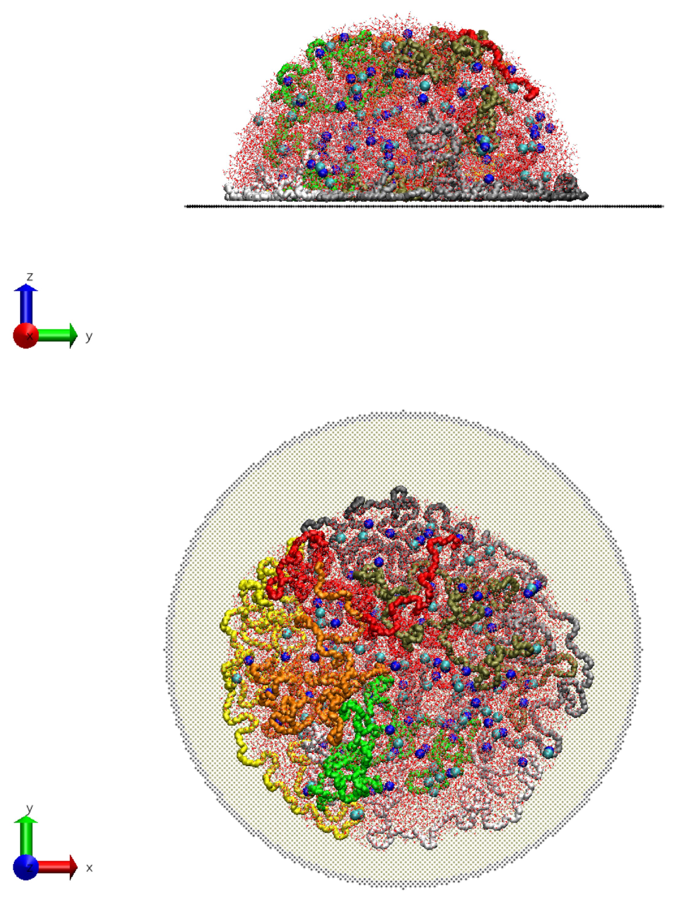
A droplet of polymer solution residing on the solid underlay before the electric field was applied (upper panel—side view, lower panel—top view). Composition of the particular system displayed is: 23,719 water molecules (O atoms red, H gray), eight 10.55-kDa poly(ethylene glycol) (PEG) chains (distinguished by different colors from one another), and 72 sodium chloride ion pairs (Na—blue spheres, Cl—cyan spheres). Graphics made by Visual Molecular Dynamics [46].
Figure 3.
A droplet of polymer solution residing on the solid underlay before the electric field was applied (upper panel—side view, lower panel—top view). Composition of the particular system displayed is: 23,719 water molecules (O atoms red, H gray), eight 10.55-kDa poly(ethylene glycol) (PEG) chains (distinguished by different colors from one another), and 72 sodium chloride ion pairs (Na—blue spheres, Cl—cyan spheres). Graphics made by Visual Molecular Dynamics [46].

Figure 4.
Schematics of the measuring device. V1—high-voltage direct-current power supply, S1—switch, D—droplet of polymer solution placed on a rod or needle metal electrode, C—collector electrode, R1—resistor (15 G), R2—resistor (1.1 M), R3—resistor (10 k). The schematics were made with Scheme-it [51].

Figure 5.
Photographs of initial droplets, just before the electric field was applied. (a) droplet at vertical working electrode in setup I. (b) A droplet at horizontal working electrode in setup II. Photographs were exported from the record of the Olympus i-SPEED 720 high-speed camera using i-SPEED Software Suite [52].

Figure 6.
(a) An example of a record from the oscilloscope and its analysis. Blue curve (channel 1)—raw voltage signal; Red curve (channel 2)—raw current signal measured as voltage on resistor R3 (see Figure 4). Tops of the rising edges of voltage and current signals are marked by vertical dashed lines. The reading 32.40 ms corresponds to their time difference. The high-amplitude damped oscillation of current accompanying the rise of voltage are merely the artifact of voltage discontinuity at closing the switch and do not indicate any response of the sample. Blank measurement without the droplet shows the same feature in the current signal, see (b) (voltage was not recorded). Setup I was used at air temperature 24.0 C and relative humidity 60%. Images were exported from the oscilloscope and edited by Inkscape [14]. Vertical offsets of the curves are arbitrarily adjusted for viewing purposes.

Figure 7.
Snapshots from a production trajectory of the system with eight 10.55-kDa chains and no ion pairs under the applied electric field of 1.5 V/nm—time evolution from 0 to 78 ps in 6-ps steps. As a visual aid, a 10-by-10-nm grid is displayed. For color scheme see Figure 3. Graphics made with Visual Molecular Dynamics [46] and ImageMagick [55].

Figure 8.
Snapshots from a production trajectory of the system with eight 10.55-kDa chains and 72 NaCl ion pairs under 1.5 V/nm—time evolution from 0 to 78 ps in 6-ps steps. As a visual aid, a 10-by-10-nm grid is displayed. For color scheme see Figure 3. Graphics made with Visual Molecular Dynamics [46] and ImageMagick [55].

Figure 9.
Snapshots from a production trajectory at 42 ps of the systems with eight 10.55-kDa chains without ions (left) and with 72 NaCl ion pairs (right) under 1.5 V/nm. In the right panel, the sodium ions (blue spheres) escaping the droplet are visible. As a visual aid, a 10-by-10-nm grid is displayed. For color scheme see Figure 3. Graphics made with Visual Molecular Dynamics [46].

Figure 10.
Mass transported through the plane at nm as a function of production time for samples with 5.26-kDa PEG chains under 1.5 V/nm. Curves correspond to different numbers of 5.26-kDa PEG chains and NaCl ion pairs, see the legend. Plotted with gnuplot [56].
Figure 10.
Mass transported through the plane at nm as a function of production time for samples with 5.26-kDa PEG chains under 1.5 V/nm. Curves correspond to different numbers of 5.26-kDa PEG chains and NaCl ion pairs, see the legend. Plotted with gnuplot [56].

Figure 11.
Mass transported through the plane at nm as a function of production time for samples with 10.55-kDa PEG chains under 1.5 V/nm. Curves correspond to different numbers of chains and NaCl ion pairs, see the legend. Plotted with gnuplot [56].
Figure 11.
Mass transported through the plane at nm as a function of production time for samples with 10.55-kDa PEG chains under 1.5 V/nm. Curves correspond to different numbers of chains and NaCl ion pairs, see the legend. Plotted with gnuplot [56].

Figure 12.
Mass transported through the plane at nm as a function of production time for different intensities of the applied electric field (color coded, see the legend). Samples with eight 5.26-kDa PEG chains and 0 (full line), 18 (short-dashed line), or 36 (long-dashed line) NaCl ion pairs are used. Plotted with gnuplot [56].

Figure 13.
Mass of PEG transported through the plane at nm as a function of production time for samples with 5.26-kDa PEG chains under 1.5 V/nm. Curves correspond to different numbers of 5.26-kDa PEG chains and NaCl ion pairs, see the legend. Plotted with gnuplot [56].
Figure 13.
Mass of PEG transported through the plane at nm as a function of production time for samples with 5.26-kDa PEG chains under 1.5 V/nm. Curves correspond to different numbers of 5.26-kDa PEG chains and NaCl ion pairs, see the legend. Plotted with gnuplot [56].

Figure 14.
Mass of PEG transported through the plane at nm as a function of production time for samples with 10.55-kDa PEG chains under 1.5 V/nm. Curves correspond to different numbers of chains and NaCl ion pairs, see the legend. Plotted with gnuplot [56].
Figure 14.
Mass of PEG transported through the plane at nm as a function of production time for samples with 10.55-kDa PEG chains under 1.5 V/nm. Curves correspond to different numbers of chains and NaCl ion pairs, see the legend. Plotted with gnuplot [56].

Figure 15.
Production times at which the total mass transfer through the plane at z = 20 nm exceeded 2000 Da vs. number of chains for different numbers of NaCl ion pairs (see the legend) under 1.5 V/nm. (a) 5.26-kDa PEG chains. (b) 10.55-kDa PEG chains. Graphs made by Gnumeric [57].
Figure 15.
Production times at which the total mass transfer through the plane at z = 20 nm exceeded 2000 Da vs. number of chains for different numbers of NaCl ion pairs (see the legend) under 1.5 V/nm. (a) 5.26-kDa PEG chains. (b) 10.55-kDa PEG chains. Graphs made by Gnumeric [57].

Figure 16.
Production times at which the mass transfer of PEG through the plane at z = 20 nm exceeded 500 Da vs. number of chains for different numbers of NaCl ion pairs (see the legend) under 1.5 V/nm. (a) 5.26-kDa PEG chains. (b) 10.55-kDa PEG chains. Graphs made by Gnumeric [57].
Figure 16.
Production times at which the mass transfer of PEG through the plane at z = 20 nm exceeded 500 Da vs. number of chains for different numbers of NaCl ion pairs (see the legend) under 1.5 V/nm. (a) 5.26-kDa PEG chains. (b) 10.55-kDa PEG chains. Graphs made by Gnumeric [57].

Figure 17.
Production times at which the total mass transfer through the plane at nm exceeded 2000 Da vs. the intensity of electric field for different numbers of NaCl ion pairs (see the legend). Systems with eight 5.26-kDa chains were used. Graph made by Gnumeric [57].
Figure 17.
Production times at which the total mass transfer through the plane at nm exceeded 2000 Da vs. the intensity of electric field for different numbers of NaCl ion pairs (see the legend). Systems with eight 5.26-kDa chains were used. Graph made by Gnumeric [57].

Figure 18.
The z-component of the velocity of PEG’s center of mass as a function of production time for samples with 5.26-kDa PEG chains under 1.5 V/nm. Curves correspond to different numbers of PEG chains and NaCl ion pairs, see the legend. Plotted with gnuplot [56].
Figure 18.
The z-component of the velocity of PEG’s center of mass as a function of production time for samples with 5.26-kDa PEG chains under 1.5 V/nm. Curves correspond to different numbers of PEG chains and NaCl ion pairs, see the legend. Plotted with gnuplot [56].

Figure 19.
The z-component of the velocity of PEG’s center of mass as a function of production time for samples with 10.55-kDa PEG chains under 1.5 V/nm. Curves correspond to different numbers of PEG chains and NaCl ion pairs, see the legend. Plotted with gnuplot [56].
Figure 19.
The z-component of the velocity of PEG’s center of mass as a function of production time for samples with 10.55-kDa PEG chains under 1.5 V/nm. Curves correspond to different numbers of PEG chains and NaCl ion pairs, see the legend. Plotted with gnuplot [56].

Figure 20.
The z-component, Mz, of dipole moments generated by PEG/water molecules (blue) and ions (magenta) for different numbers of NaCl ion pairs (distinguished by dashing patterns, see the legend) under 1.5 V/nm. Systems with (a) eight or (b) sixteen 5.26-kDa PEG chains were used. Plotted with gnuplot [56].

Figure 21.
The z-component, Mz, of dipole moments generated by molecules (blue) and ions (magenta) for different numbers of NaCl ion pairs (distinguished by dashing patterns, see the legend) under 1.5 V/nm. Systems with (a) four or (b) eight 10.55-kDa PEG chains were used. Plotted with gnuplot [56].

Figure 22.
The z-component, , of dipole moments generated by molecules (blue) and ions (magenta) for different intensities of the applied field (distinguished by line colors according to the legend). Results for the system with eight 5.26-kDa PEG chains and 18 NaCl ion pairs are shown. Plotted with gnuplot [56].

Figure 23.
The average rates of evaporation of water molecules under 1.5 V/nm through the indicated intervals of production time: 0–36 ps (first row), 36–72 ps (second row), and 0–72 ps (third row). Left column—5.26-kDa chains, right column—10.55-kDa chains. Results for different numbers of PEG chains (horizontal axis) and different numbers of NaCl ion pairs (colors in the legend) are shown. Each bar represents a result of a single production trajectory. Graphs made by Gnumeric [57].

Figure 24.
The energy dissipated from ions divided by the Boltzmann constant, kB, as a function of production time for samples with (a) 5.26-kDa and (b) 10.55-kDa PEG chains. Curves correspond to different numbers of PEG chains and NaCl ion pairs, see the legend. Plotted with gnuplot [56].
Figure 24.
The energy dissipated from ions divided by the Boltzmann constant, kB, as a function of production time for samples with (a) 5.26-kDa and (b) 10.55-kDa PEG chains. Curves correspond to different numbers of PEG chains and NaCl ion pairs, see the legend. Plotted with gnuplot [56].

Figure 25.
The solvent evaporation rate vs the dissipated energy divided by kB for (a) 0–36 ps and (b) 36–72 ps of production time. Simulation data (symbols) are shown along with a linear least-square regression (line). Pearson’s correlation coefficients, r, are also displayed alongside the regression lines. Results for 8 or 16 5.26-kDa PEG chains (open or filled blue circles), and for 4 or 8 10.55-kDa PEG chains (open or filled green squares) are shown. Plotted by Gnumeric [57] and edited with Inkscape [14].

Figure 26.
The solvent evaporation rate vs the dissipated energy divided by for 0–72 ps of production time. Simulation data (symbols) are shown along with a linear least-square regression (line). Pearson’s correlation coefficients, r, are also displayed alongside the regression lines. Results for 8 or 16 5.26-kDa PEG chains (open or filled blue circles), and for 4 or 8 10.55-kDa PEG chains (open or filled green squares) are shown. Plotted by Gnumeric [57] and edited with Inkscape [14].

Figure 27.
The experimental instability onset times determined from oscilloscopic voltage–current delays. Mean values of 10 measurements are plotted, error bars correspond to standard deviations of the mean. Graph made by Gnumeric [57].
Figure 27.
The experimental instability onset times determined from oscilloscopic voltage–current delays. Mean values of 10 measurements are plotted, error bars correspond to standard deviations of the mean. Graph made by Gnumeric [57].

Figure 28.
(a) Current through electrodes as a function of time measured from the introduction of voltage. The inset shows the details of the current onset. (b) A sequence of photographs taken at the times marked by blue vertical lines (with matching Roman numerals) in the inset above. Experiment was done in setup I with sample b0 at 24.6 C and relative humidity 41%. Photographs were exported from the record of the Olympus i-SPEED 720 high-speed camera using i-SPEED Software Suite [52].

Figure 29.
(a) Current through electrodes as a function of time measured from the introduction of voltage. (b) A sequence of photographs taken at the times corresponding to blue vertical lines (with matching Roman numerals) in the plot above. The experiment was done in setup I with sample a0 at 24.6 C and 41% relative humidity. Photographs were exported from the record of the Olympus i-SPEED 720 high-speed camera using i-SPEED Software Suite [52].

Figure 30.
A spindle-like formation before the detachment from the mother droplet. The jet emanating from a tip of the spindle is visible on the left. The experiment was done in setup II with solution a0 at 22.0 C and relative humidity 40%. Photographs were exported from the record of the Olympus i-SPEED 720 high-speed camera using i-SPEED Software Suite [52].

Figure 31.
Formation and decay of the jet. Photographs are taken 0.1 ms apart. The experiment was done in setup II with solution a0 at 22.0 C and relative humidity 40%. Photographs were exported from the record of the Olympus i-SPEED 720 high-speed camera using i-SPEED Software Suite [52].
Figure 31.
Formation and decay of the jet. Photographs are taken 0.1 ms apart. The experiment was done in setup II with solution a0 at 22.0 C and relative humidity 40%. Photographs were exported from the record of the Olympus i-SPEED 720 high-speed camera using i-SPEED Software Suite [52].

Figure 32.
Formation of a splaying jet and its decay. Photographs are taken 0.1 ms apart. The experiment was done in setup II with solution a0 at 22.0 C and relative humidity 40%. Photographs were exported from the record of the Olympus i-SPEED 720 high-speed camera using i-SPEED Software Suite [52].


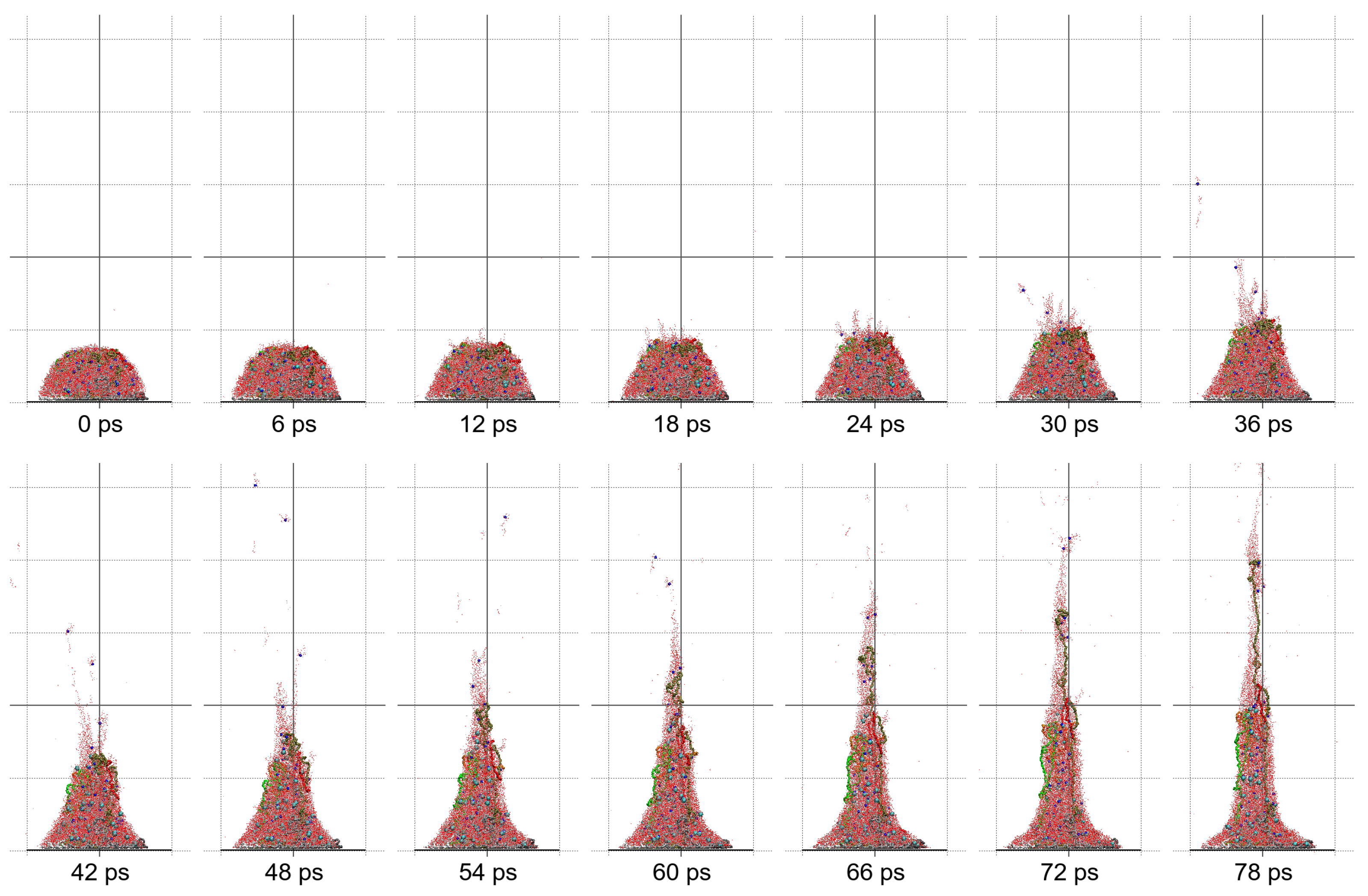
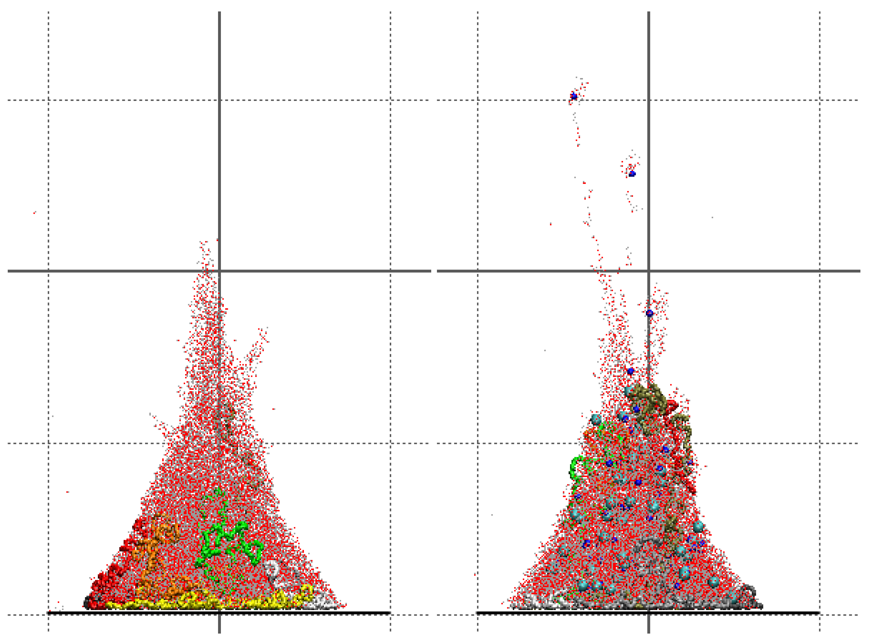
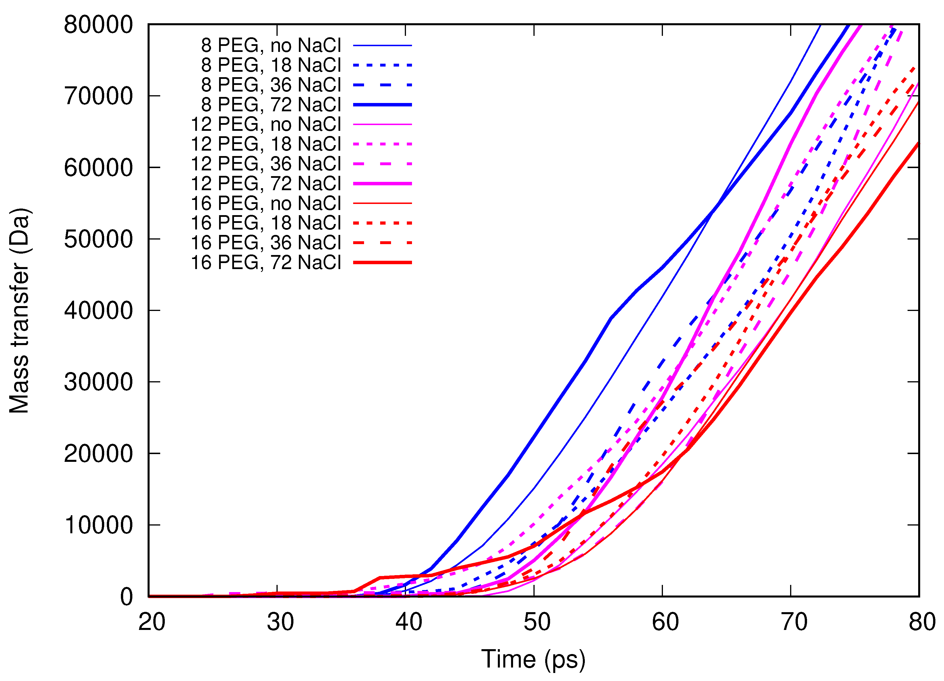
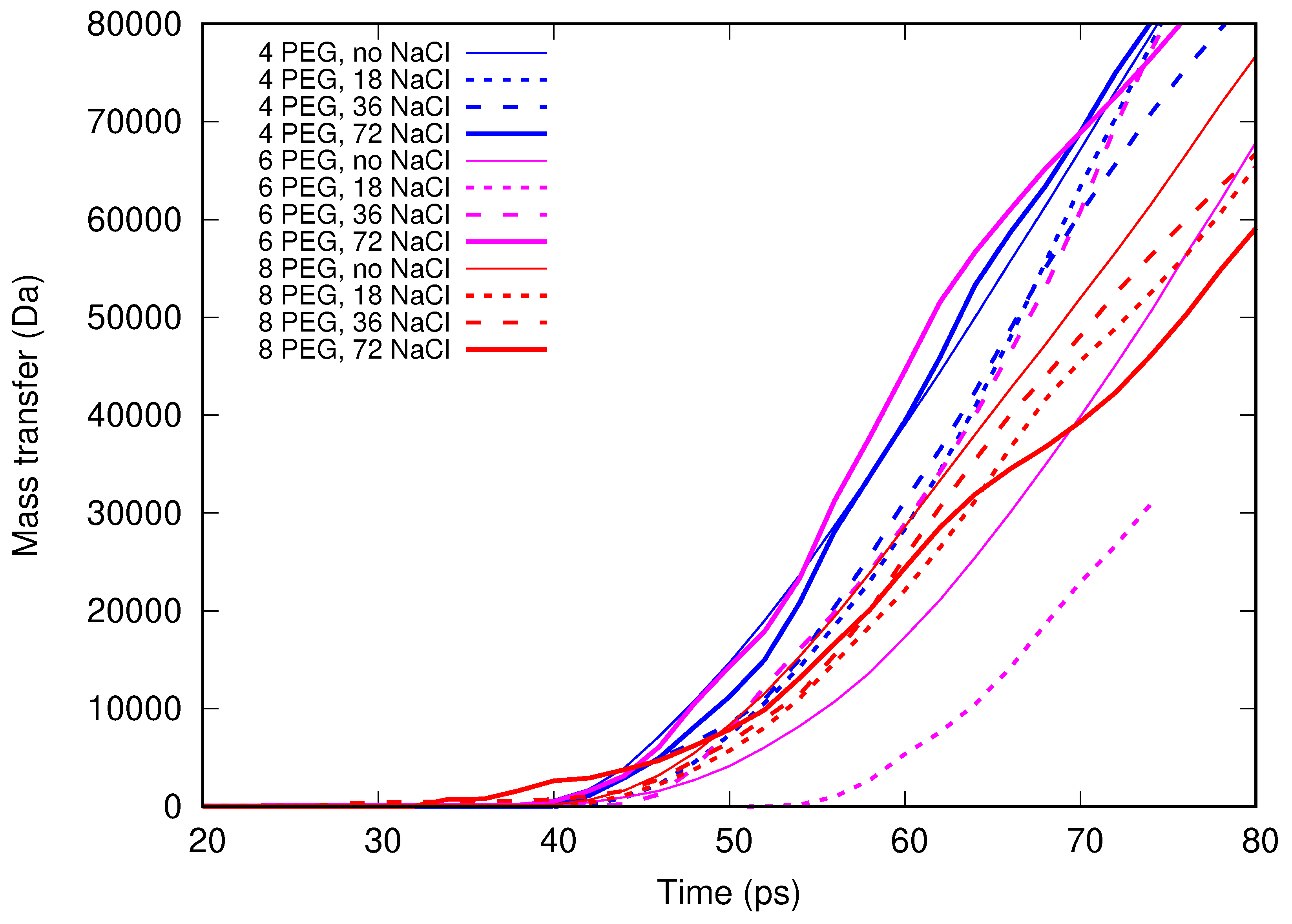
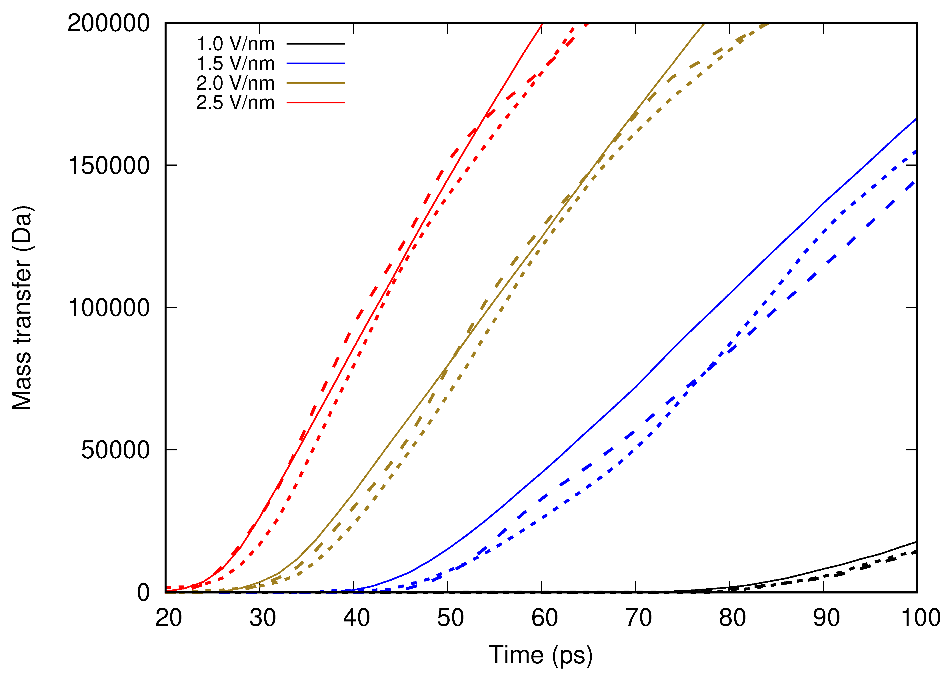
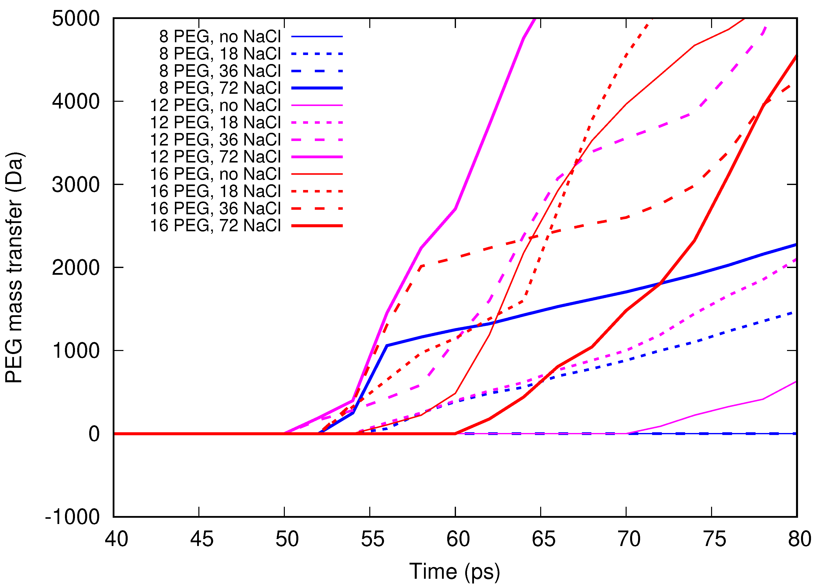
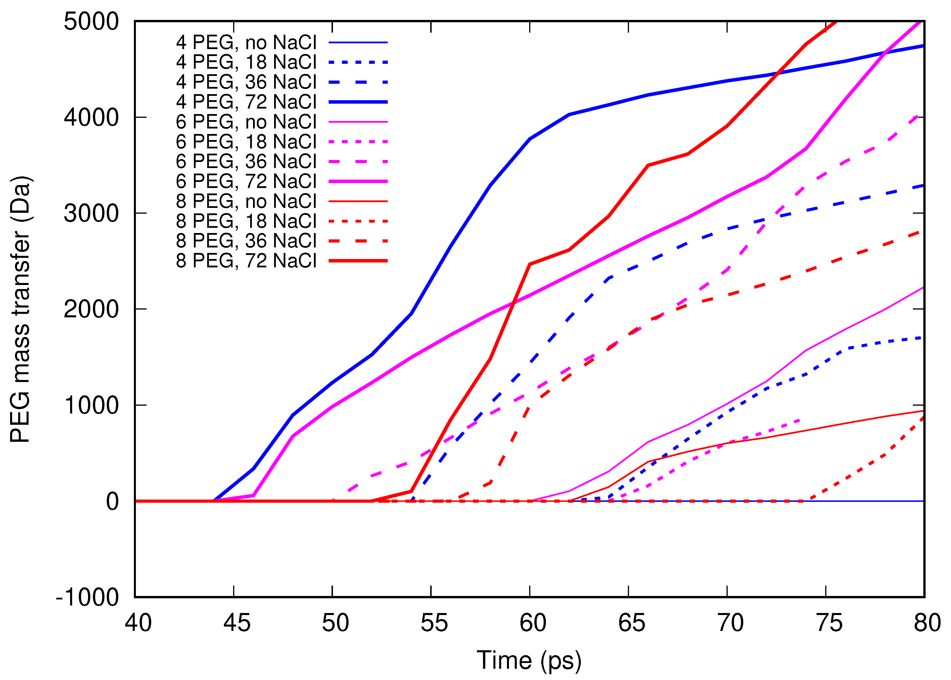
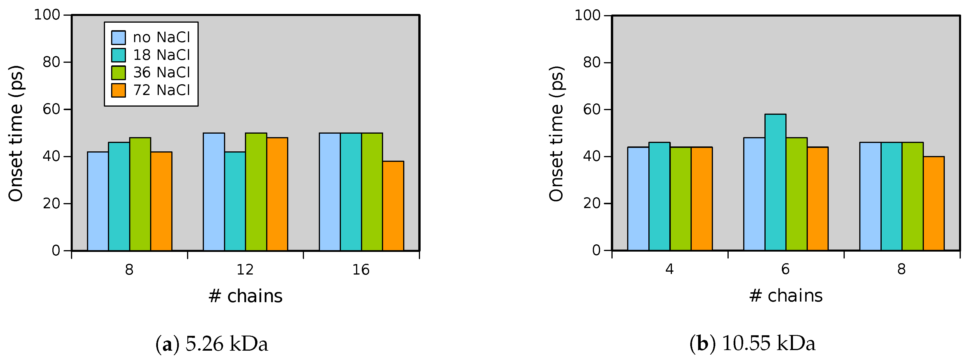
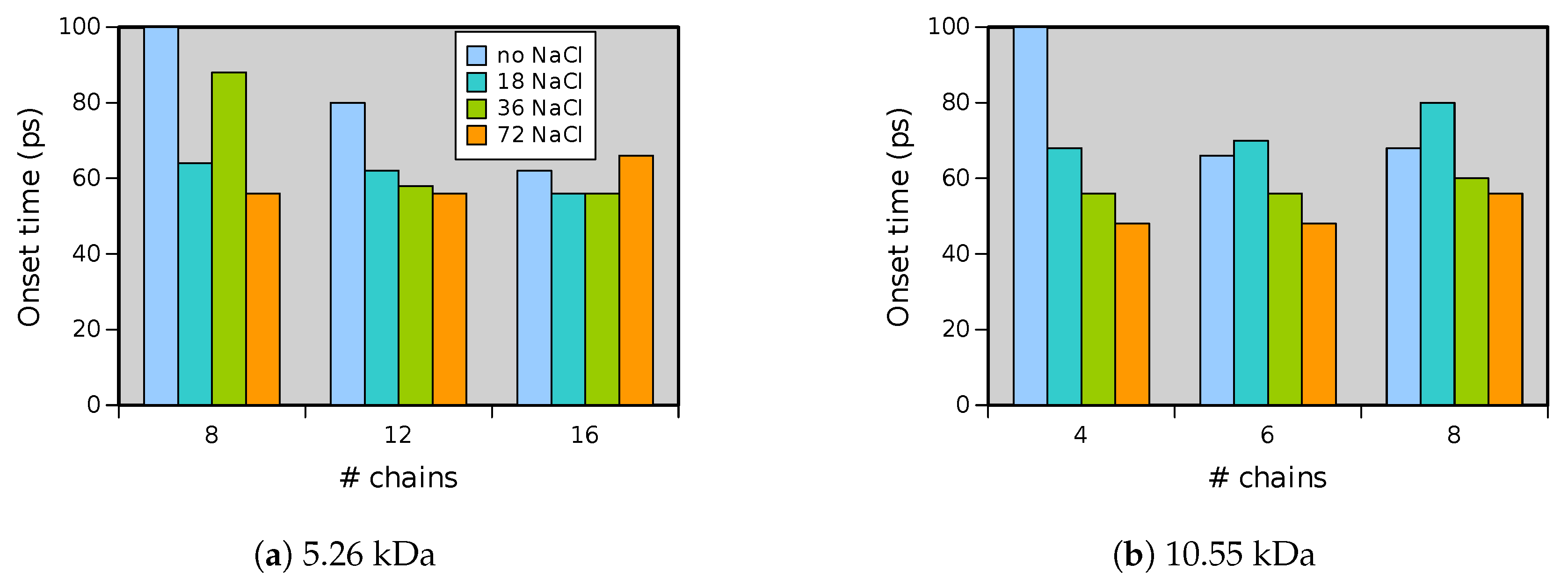
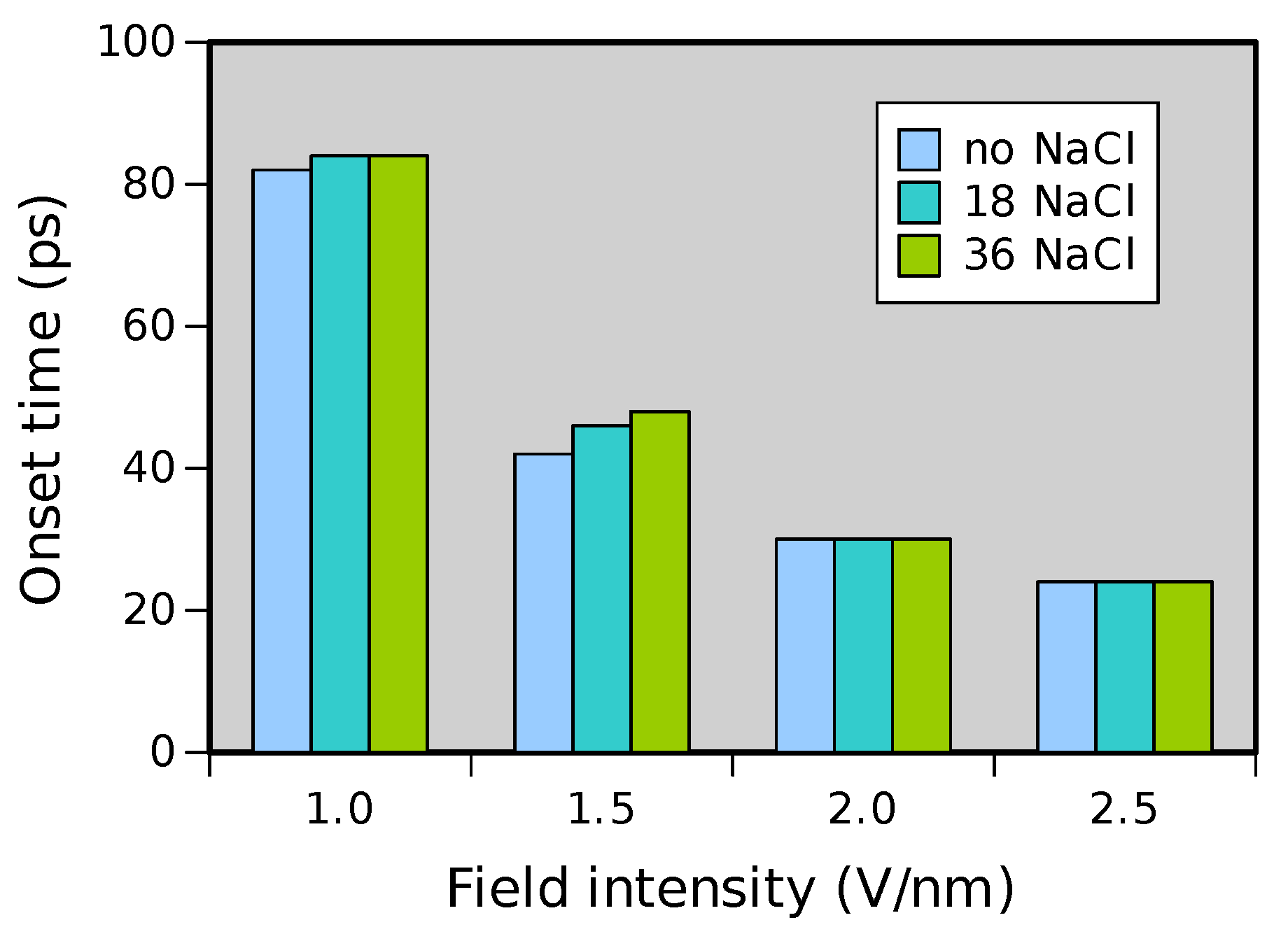
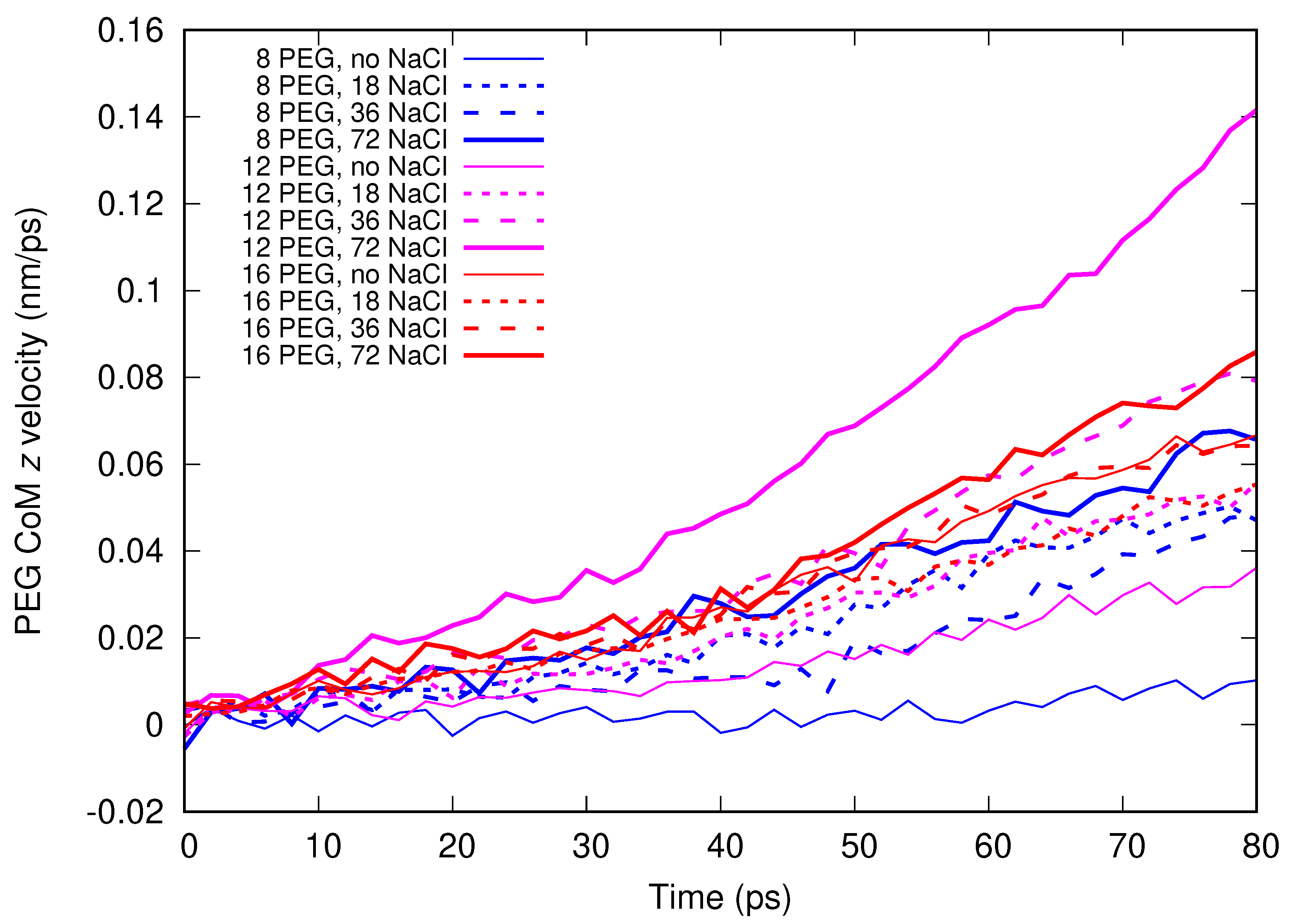
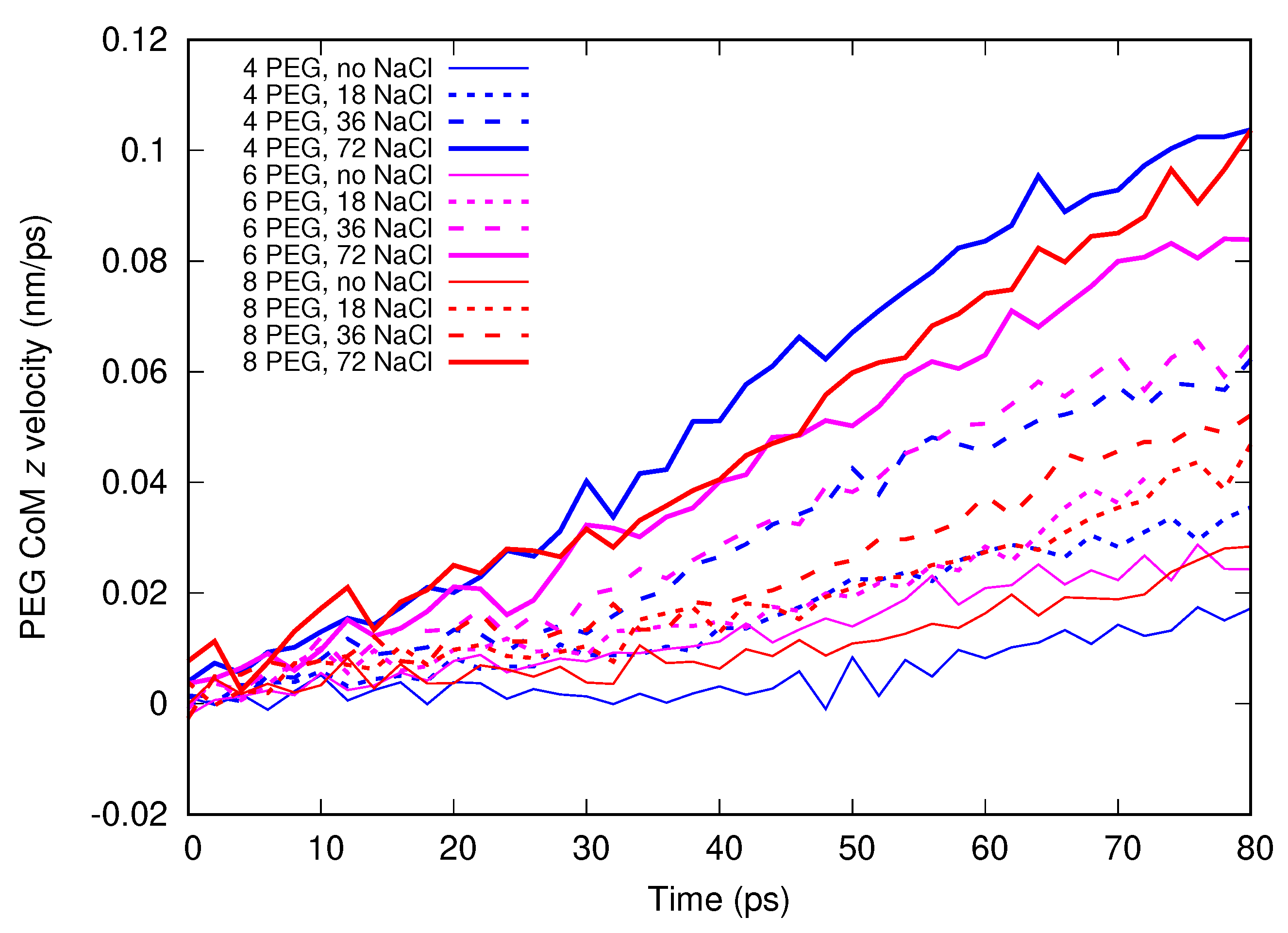
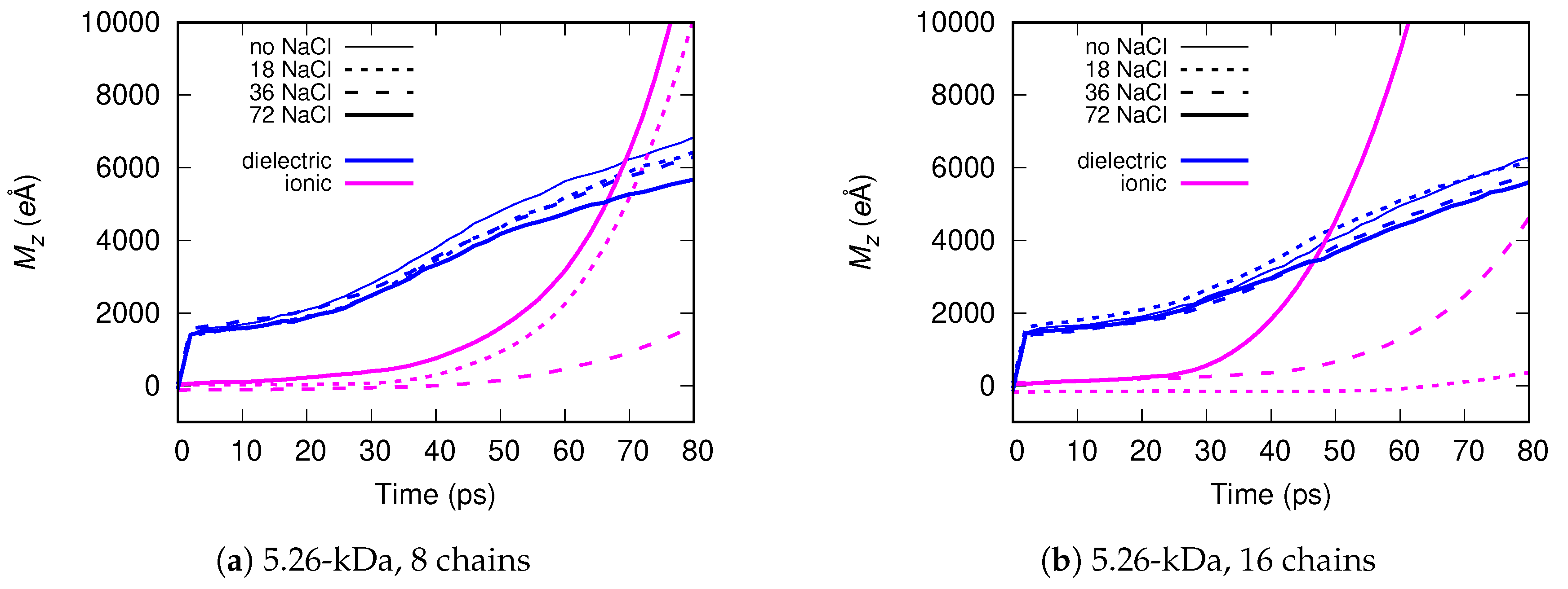
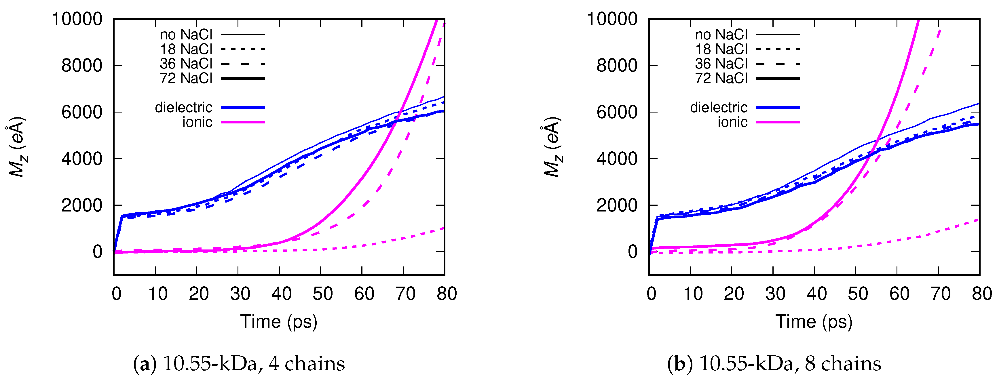
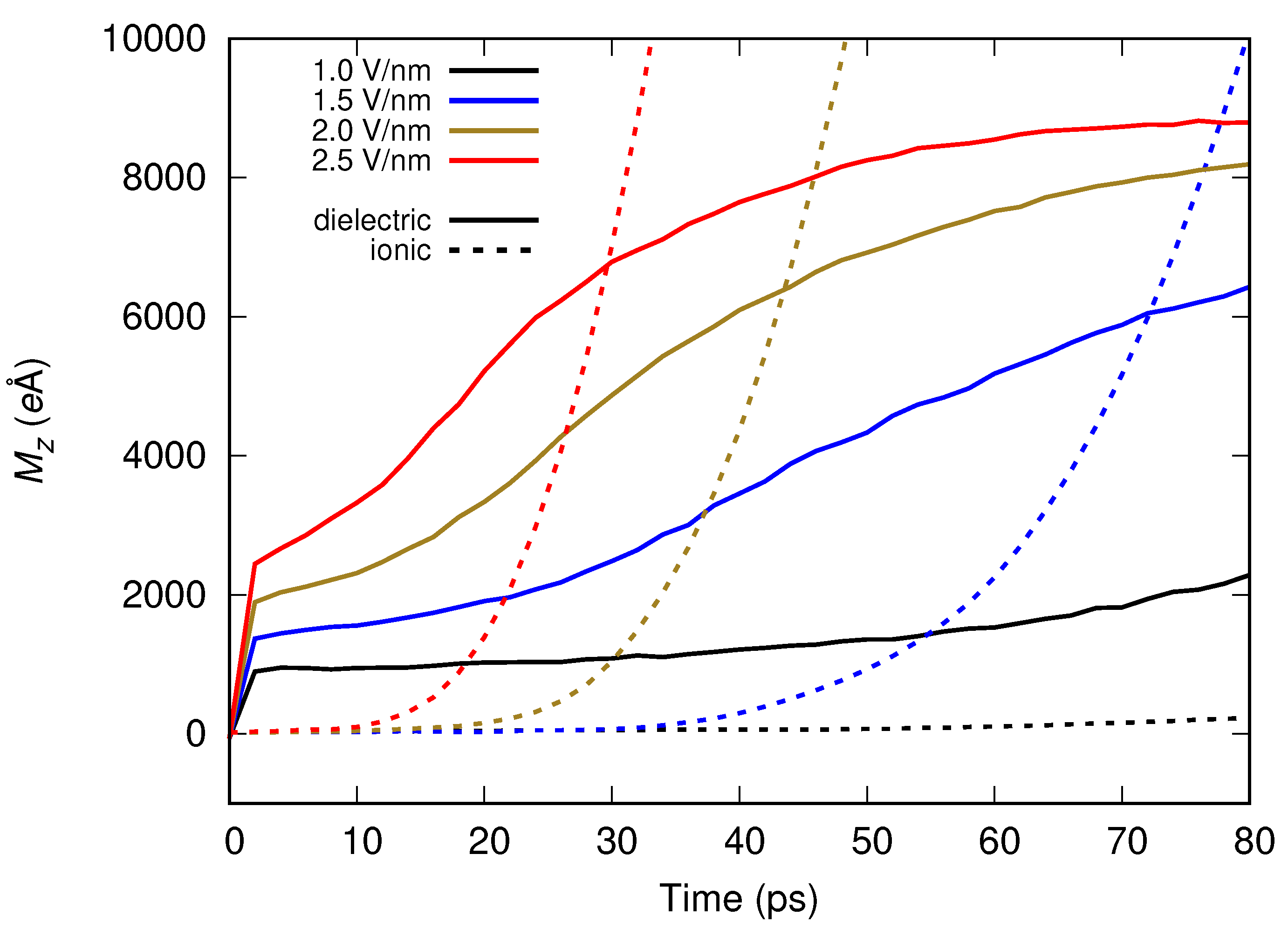
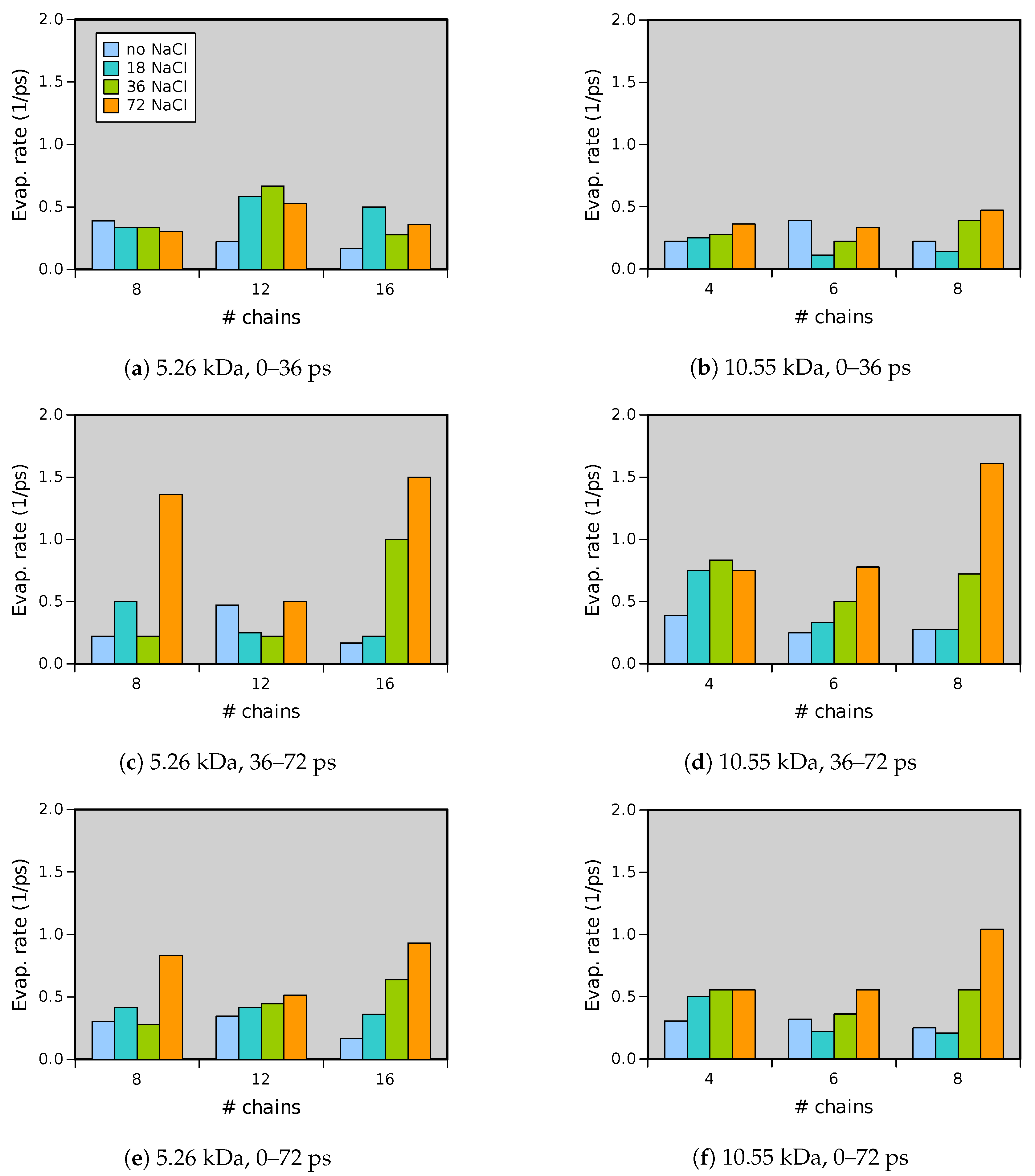
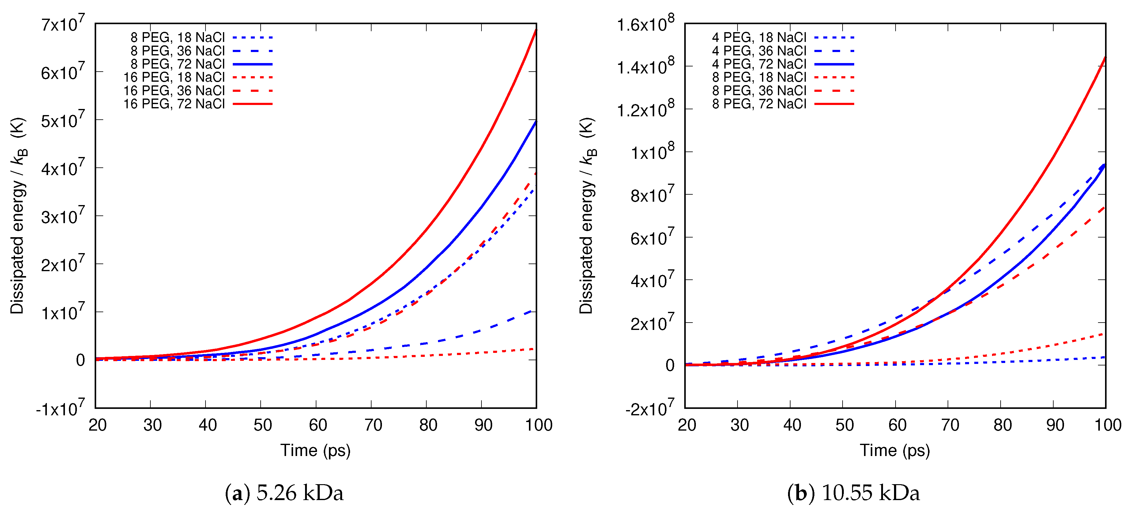
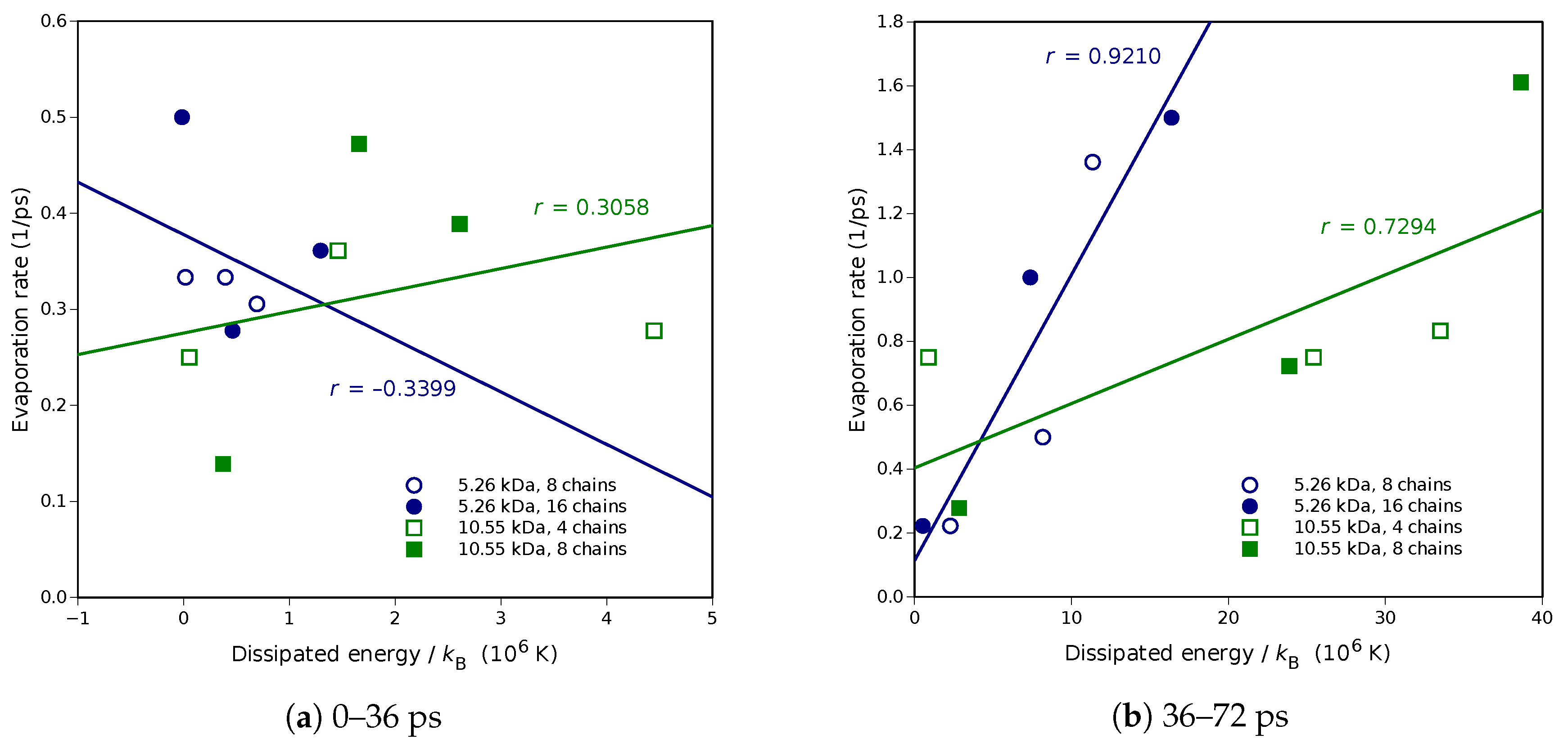
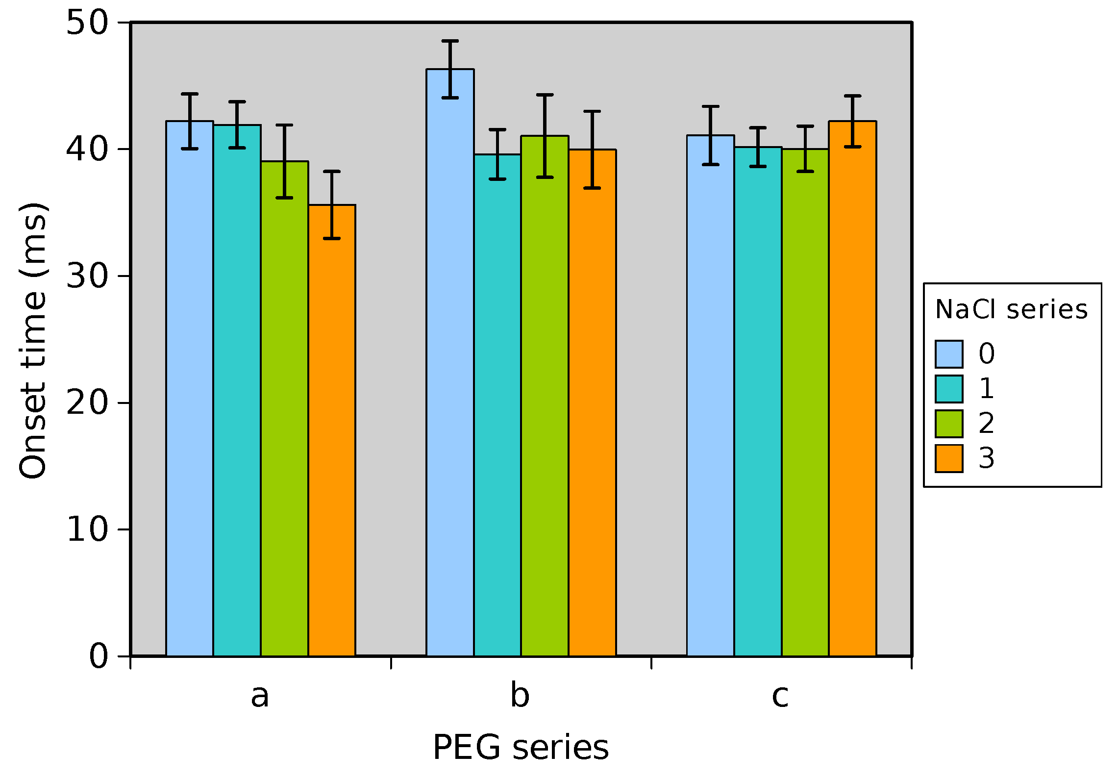
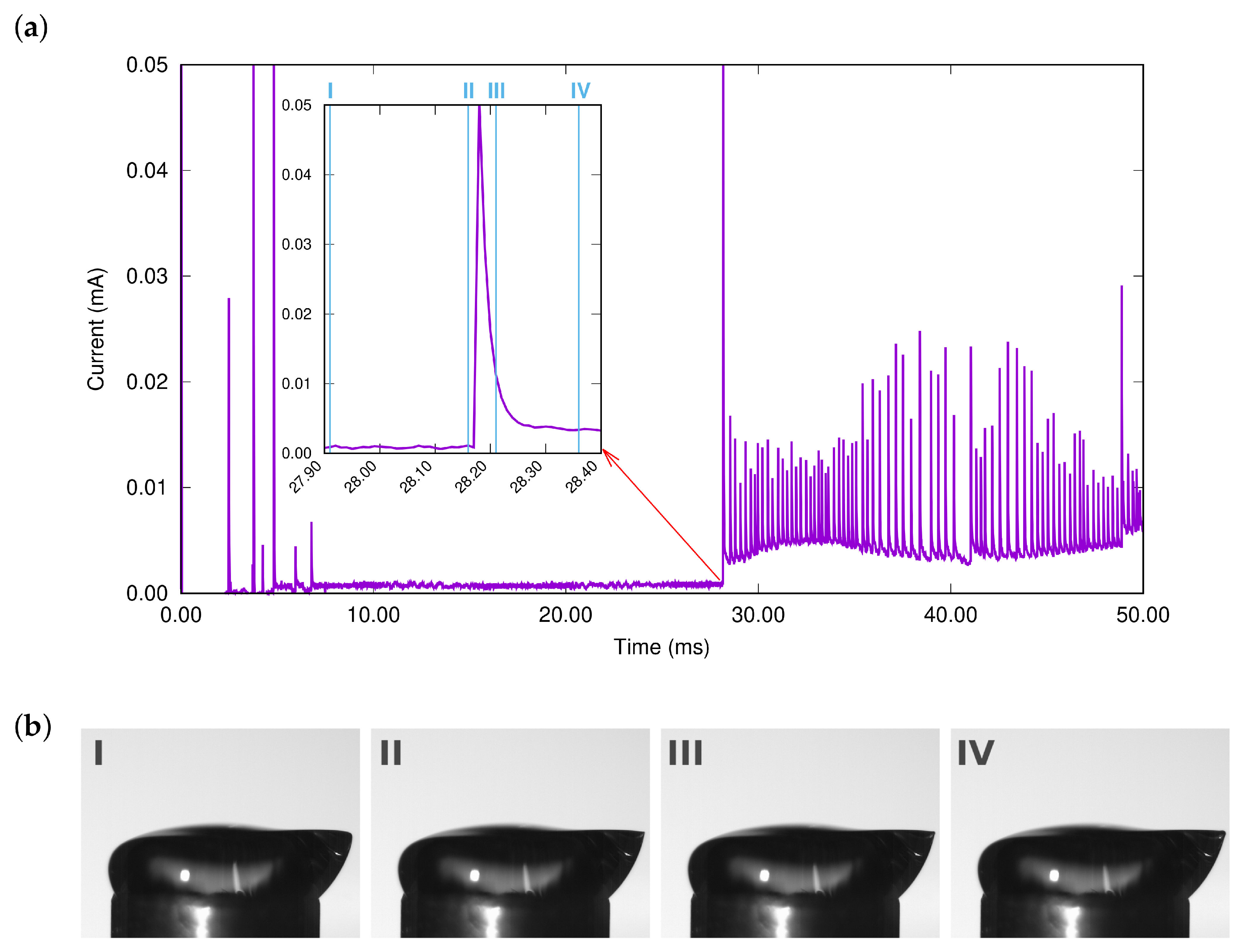
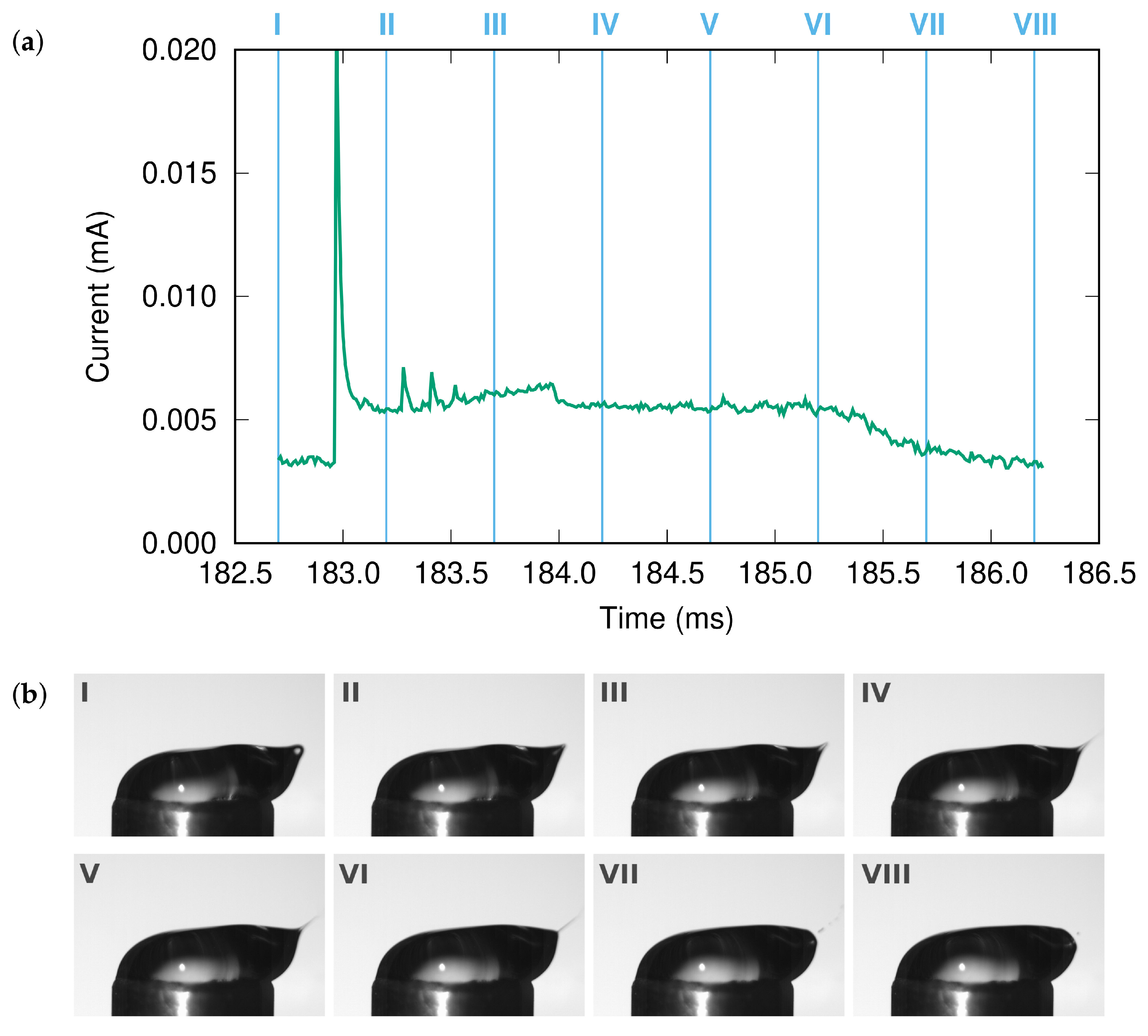
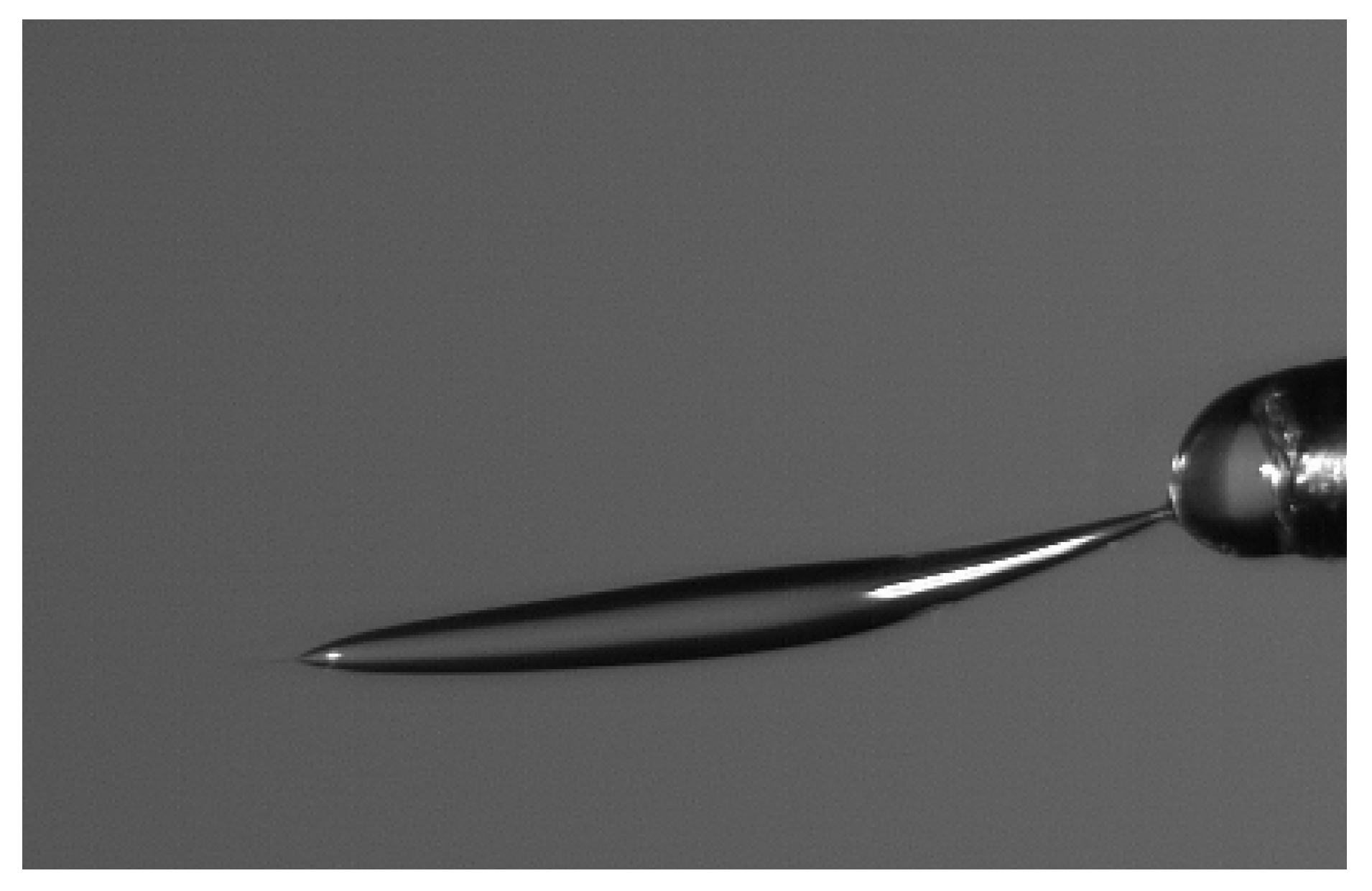
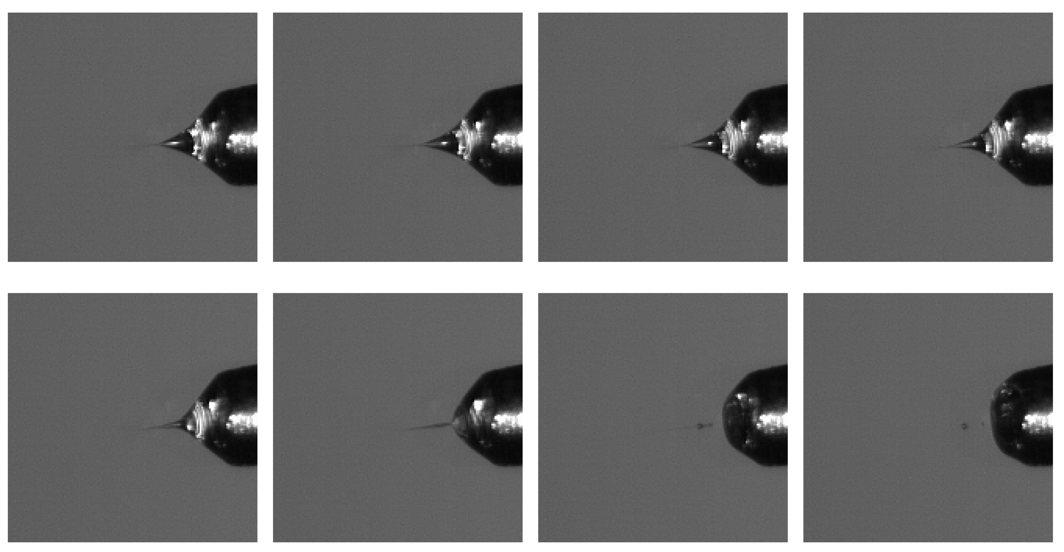
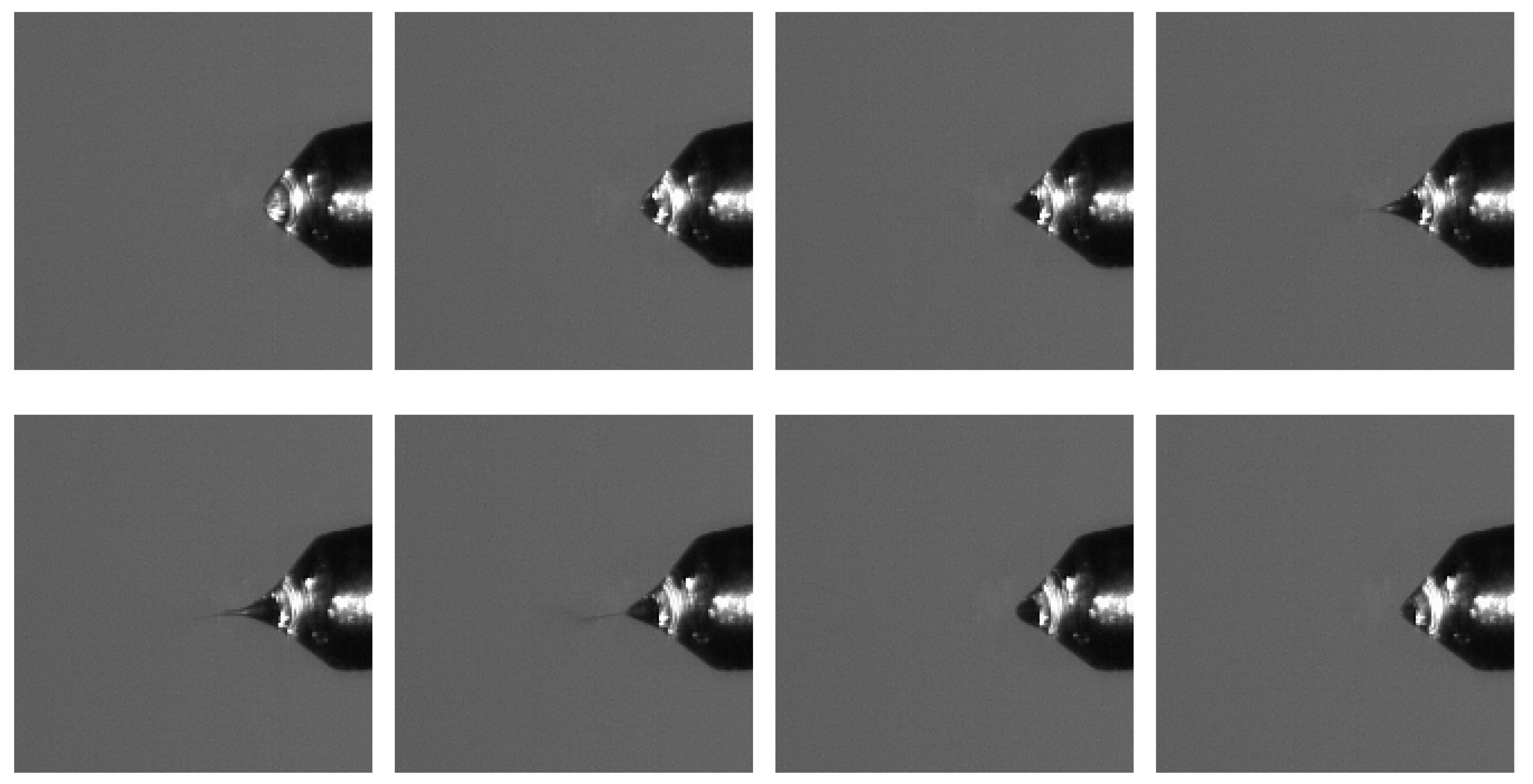
Table 1.
Technical parameters of experimental measurements.
| Parameter | Experimental Setup | |
|---|---|---|
| I | II | |
| working electrode diameter | 10 mm | 1.1 mm |
| working electrode axis | vertical | horizontal |
| est. droplet volume | 0.2 mL | 0.5 L |
| collector shape | disc | square |
| collector dimensions | ⌀ 120 mm | mm |
| collector material | aluminium | steel |
| electrode separation | 70 mm | 100 mm |
| voltage | 20 kV | 10 kV |
| current limit | 0.15 mA | 0.10 mA |
Table 2.
Numbers of water molecules in production runs of all the simulated systems.
| 0 | 18 | 36 | 72 | |
|---|---|---|---|---|
| 8 | 23,684 | 23,682 | 23,684 | 23,695 |
| 12 | 23,687 | 23,695 | 23,693 | 23,707 |
| 16 | 23,692 | 23,682 | 23,686 | 23,703 |
| 10,547 | ||||
| 4 | 23,703 | 23,708 | 23,704 | 23,718 |
| 6 | 23,722 | 23,717 | 23,713 | 23,730 |
| 8 | 23,706 | 23,709 | 23,700 | 23,719 |
Table 3.
Weight fractions (%) of PEG in production runs of all the simulated systems.
| 0 | 18 | 36 | 72 | |
|---|---|---|---|---|
| 8 | 8.98 | 8.96 | 8.94 | 8.89 |
| 12 | 12.89 | 12.85 | 12.83 | 12.77 |
| 16 | 16.47 | 16.44 | 16.41 | 16.33 |
| 10,547 | ||||
| 4 | 8.99 | 8.97 | 8.95 | 8.91 |
| 6 | 12.90 | 12.87 | 12.85 | 12.78 |
| 8 | 16.50 | 16.46 | 16.43 | 16.35 |
Table 4.
Molalities of sodium chloride (mol/kg) in production runs of all the simulated systems.
| 0 | 18 | 36 | 72 | |
|---|---|---|---|---|
| 8 | 0.00000 | 0.0422 | 0.0844 | 0.1687 |
| 12 | 0.00000 | 0.0422 | 0.0843 | 0.1686 |
| 16 | 0.00000 | 0.0422 | 0.0844 | 0.1686 |
| 10,547 | ||||
| 4 | 0.00000 | 0.0421 | 0.0843 | 0.1685 |
| 6 | 0.00000 | 0.0421 | 0.0843 | 0.1684 |
| 8 | 0.00000 | 0.0421 | 0.0843 | 0.1685 |
Table 5.
Production times (ps) at which the total mass transfer through the plane at nm exceeded 2000 Da under 1.5 V/nm.
Table 5.
Production times (ps) at which the total mass transfer through the plane at nm exceeded 2000 Da under 1.5 V/nm.
| 0 | 18 | 36 | 72 | |
|---|---|---|---|---|
| 8 | 42 | 46 | 48 | 42 |
| 12 | 50 | 42 | 50 | 48 |
| 16 | 50 | 50 | 50 | 38 |
| 10,547 | ||||
| 4 | 44 | 46 | 44 | 44 |
| 6 | 48 | 58 | 48 | 44 |
| 8 | 46 | 46 | 46 | 40 |
Table 6.
Production times (ps) at which the mass transfer of PEG through the plane at nm exceeded 500 Da under 1.5 V/nm.
Table 6.
Production times (ps) at which the mass transfer of PEG through the plane at nm exceeded 500 Da under 1.5 V/nm.
| 0 | 18 | 36 | 72 | |
|---|---|---|---|---|
| 8 | >100 | 64 | 88 | 56 |
| 12 | 80 | 62 | 58 | 56 |
| 16 | 62 | 56 | 56 | 66 |
| 10,547 | ||||
| 4 | >100 | 68 | 56 | 48 |
| 6 | 66 | 70 | 56 | 48 |
| 8 | 68 | 80 | 60 | 56 |
Table 7.
Production times (ps) at which the total mass transfer through the plane at nm exceeded 2000 Da for different field intensities, E. Systems with eight 5.26-kDa chains were used.
Table 7.
Production times (ps) at which the total mass transfer through the plane at nm exceeded 2000 Da for different field intensities, E. Systems with eight 5.26-kDa chains were used.
| E (V/nm) | |||
|---|---|---|---|
| 0 | 18 | 36 | |
| 1.0 | 82 | 84 | 84 |
| 1.5 | 42 | 46 | 48 |
| 2.0 | 30 | 30 | 30 |
| 2.5 | 24 | 24 | 24 |
Table 8.
Weight fractions (%) of PEG in the solutions used in experiments.
| PEG Series | NaCl Series | |||
|---|---|---|---|---|
| 0 | 1 | 2 | 3 | |
| a | 9.01 | 8.99 | 8.97 | 8.91 |
| b | 12.89 | 12.86 | 12.84 | 12.78 |
| c | 16.46 | 16.42 | 16.39 | 16.33 |
Table 9.
Molalities of sodium chloride (moles of NaCl per kg of water) in solutions used in experiments.
Table 9.
Molalities of sodium chloride (moles of NaCl per kg of water) in solutions used in experiments.
| PEG Series | NaCl Series | |||
|---|---|---|---|---|
| 0 | 1 | 2 | 3 | |
| a | 0.0000 | 0.0429 | 0.0838 | 0.1694 |
| b | 0.0000 | 0.0427 | 0.0838 | 0.1693 |
| c | 0.0000 | 0.0428 | 0.0839 | 0.1695 |
Table 10.
Conductivities of all samples (S/cm) at 21 C. Mean values calculated from 3 measurements are given along with standard deviations of the mean.
Table 10.
Conductivities of all samples (S/cm) at 21 C. Mean values calculated from 3 measurements are given along with standard deviations of the mean.
| PEG Series | NaCl Series | |||
|---|---|---|---|---|
| 0 | 1 | 2 | 3 | |
| a | 35 ± 1 | 2019 ± 54 | 3703 ± 25 | 6573 ± 31 |
| b | 37 ± 1 | 1845 ± 5 | 3343 ± 6 | 5923 ± 67 |
| c | 38 ± 1 | 1614 ± 4 | 2930 ± 10 | 5293 ± 21 |
Table 11.
The experimental instability onset times (ms) determined from oscilloscopic voltage–current delays. Mean values calculated from 10 measurements are given along with standard deviations of the mean. The air temperature was 24.0 C, and the relative humidity was 60%.
Table 11.
The experimental instability onset times (ms) determined from oscilloscopic voltage–current delays. Mean values calculated from 10 measurements are given along with standard deviations of the mean. The air temperature was 24.0 C, and the relative humidity was 60%.
| PEG Series | NaCl Series | |||
|---|---|---|---|---|
| 0 | 1 | 2 | 3 | |
| a | 42.20 ± 2.16 | 41.92 ± 1.82 | 39.04 ± 2.87 | 35.60 ± 2.64 |
| b | 46.30 ± 2.24 | 39.60 ± 1.95 | 41.04 ± 3.26 | 39.96 ± 3.03 |
| c | 41.08 ± 2.30 | 40.16 ± 1.52 | 40.03 ± 1.79 | 42.20 ± 2.00 |
© 2020 by the authors. Licensee MDPI, Basel, Switzerland. This article is an open access article distributed under the terms and conditions of the Creative Commons Attribution (CC BY) license (http://creativecommons.org/licenses/by/4.0/).
Share and Cite
MDPI and ACS Style
Jirsák, J.; Pokorný, P.; Holec, P.; Dědičová, Š. A Molecular-Level Picture of Electrospinning. Water 2020, 12, 2577. https://doi.org/10.3390/w12092577
AMA Style
Jirsák J, Pokorný P, Holec P, Dědičová Š. A Molecular-Level Picture of Electrospinning. Water. 2020; 12(9):2577. https://doi.org/10.3390/w12092577
Chicago/Turabian StyleJirsák, Jan, Pavel Pokorný, Pavel Holec, and Šárka Dědičová. 2020. "A Molecular-Level Picture of Electrospinning" Water 12, no. 9: 2577. https://doi.org/10.3390/w12092577
Note that from the first issue of 2016, this journal uses article numbers instead of page numbers. See further details here.