Article

Sea-Level Variability in the Gulf of Naples and the “Acqua Alta” Episodes in Ischia from Tide-Gauge Observations in the Period 2002–2019

Dipartimento di Scienze e Tecnologie, Università degli Studi di Napoli “Parthenope”, Ctr Direz Isola C4, 80143 Naples, Italy
*
Authors to whom correspondence should be addressed.
Water 2020, 12(9), 2466; https://doi.org/10.3390/w12092466
Submission received: 28 July 2020 / Revised: 30 August 2020 / Accepted: 31 August 2020 / Published: 2 September 2020
(This article belongs to the Special Issue Relative Sea-Level Changes and their Impact on Coastal Zones)

Abstract

:
This work presents an 18-year-long (2002–2019) tide-gauge dataset collected on the Island of Ischia (Gulf of Naples, Southern Tyrrhenian Sea) that can contribute to the analysis of the basic features of sea-level variability in this region. Analysis of tidal constituents shows that the Gulf of Naples is characterized by the absence of any amphidromic system. In this area, sea-level changes due to the astronomical component of the tide are generally limited to ±20 cm with respect to the mean sea level, but the impact of this variability is enhanced by global sea-level increase and the effect of regional atmospheric perturbations that might also triple sea-level variations. The effects of these events, whose frequency has increased in recent decades, has been dramatic in coastal areas where intense social and economic activity occurs, e.g., in Ischia. On interannual time scales, the results indicate that the relative sea-level rise in Ischia has a magnitude of 3.9 mm/year. Special attention is dedicated to the “acqua alta” episodes and to their linkage with long-term sea-level trends and atmospheric forcing.

1. Introduction

Sea level (SL) can change over a wide range of temporal and spatial scales. Even though available in situ observations are characterized by a sparse and uneven spatial distribution [1] that largely limits their use [2], tide-gauge records represent the main source of information about local SL variations from the last two centuries [3,4,5,6,7]. Previously, tide-gauges were mainly used for navigation issues, e.g., to observe and forecast SL variations associated with the tide, but nowadays they are also essential for evaluating oceanographic models, e.g., [8], validating satellite data [9,10], and performing instrumental calibration of satellite missions [11,12], as well as being used in the framework of long-term climatic studies. With growing comprehension of SL variation and its interaction with atmospheric variability, the importance of these records has then enlarged to coastal area management issues. A global SL rising trend has been associated with climate change and human-originated greenhouse effects, e.g., [13,14,15,16,17]. In its fifth assessment report (AR5), the Intergovernmental Panel on Climate Change (IPCC) estimated SL increases of 1.7, 2.0, and 3.2 mm/year in the periods 1901–2010, 1971–2010, and 1993–2010, respectively [18,19,20], with potential dramatic societal impacts on coastal regions [21]. In particular, AR5 indicates that the Mediterranean Sea is one of the most vulnerable regions in the world in terms of the impacts of climate change and SL rise.
The analysis of the longest tide-gauge series along the Mediterranean Sea coasts indicates a rate of SL rise of 1.1–1.3 mm/year over the 20th century [22]. This trend is not homogeneous, with a period of SL decrease after the 1960s [22] and a fast rise in SL observed since the late 1990s [23,24]. Furthermore, a high-resolution SL time series showed the existence of a seasonal signal superimposed on the long-term trend [19]. Finally, the presence of densely populated areas along the coasts and a high-value economic activity have enhanced these impacts. The Campania Region coast in the Southern Tyrrhenian Sea has been identified as one of the Italian coastal areas that is most susceptible to inundation risk [25,26,27].
Although estimations of SL trends have been retrieved on the basis of the longest tide-gauges records available, the temporal and spatial distributions of these instruments strongly affect the results. SL can significantly vary from one region to another, and a variety of processes cause local trends to deviate from the global mean rate of change [7,28]. Therefore, it is not straightforward to infer the rate of global ocean volume change from these data. It is necessary to study SL changes on a local or regional basis to determine both the long-term trend and the shorter wavelengths of the signals, as well as to understand the different geophysical processes associated with such changes [13]. These efforts could then help in distinguishing between natural and anthropogenic changes occurring in the Earth’s climate system and affecting the livelihoods of millions of people [29]. In this context, the availability of additional tide-gauge data in the Mediterranean Sea and detailed study of the Tyrrhenian sub-basins [30,31,32] is important to provide more accurate information on basin circulation and on the local SL variability and its trends.
In the Gulf of Naples (GON) in the Southern Tyrrhenian Sea (Figure 1), the University of Naples “Parthenope” manages a large weather and oceanographic monitoring network that includes weather stations, a weather radar, wave-buoys, oceanographic moorings, and a coastal high-frequency radar network. In this framework, since 2002, a tide-gauge has operated on the island of Ischia (IS). In this area, SL variability due to the purely theoretical astronomical component is ±20 cm with respect to the mean SL, but the impact of this variability is enhanced by the global SL increase and the effect of regional atmospheric perturbations that can even triple SL variations. A second tide-gauge is located in the GON at Castellammare di Stabia (CS), but it has only operated since 2011. The locations of both the instruments were planned according to the different geological histories and characteristics of the sites. Ischia is characterized by intense volcanic activity and a complex tectonic history [33], while CS is located next to the Monti Lattari carbonate reliefs that are characterized by greater stability [34].
Together with the Volturno coastal plain, Ischia and Castellammare are characterized by high economic and ecological value, due to the presence of tourist structures, farm activities, and wetland protected zones [27] that increase their vulnerability to sea level rise and storm surge.
In this study, the 18-year IS tide-gauge dataset was carefully analyzed to identify the basic features of SL variability and the interactions with the atmospheric variability and to describe the possible causes of the remarkable “acqua alta” (“high water”, hereafter AA) episodes in Ischia. To reach this aim, the IS SL data interannual variability was analyzed, and a comparison between IS tidal constants with nearby tide-gauges, including CS, was conducted. The frequency and amplitude of the AA events are discussed. The “Materials and Methods” section describes the tide-gauges, their locations, and the collected observations, as well as the air pressure data and the large scale atmospheric indices included in the analyses. Finally, future perspectives for the analysis of SL variability in the study area and improvements in the tide-gauge network are also described.

2. Materials and Methods

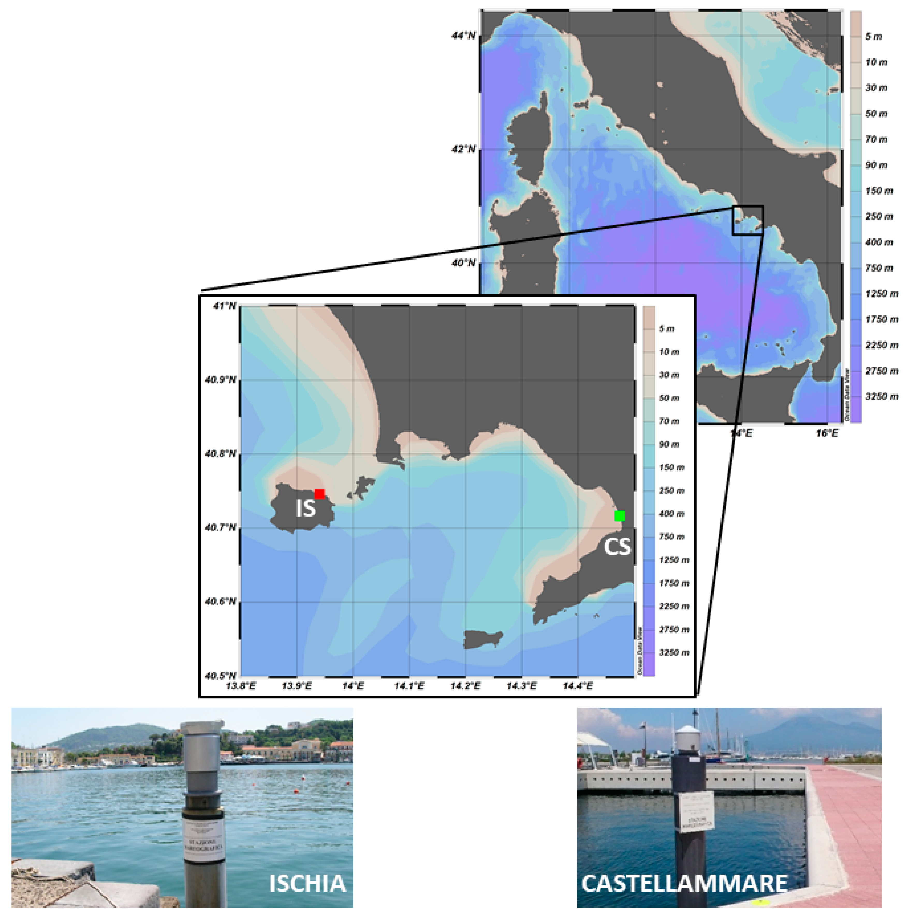
2.1. Tide-Gauge Data

A “Thalimedes” tide-gauge by OTT HydroMet (IS in Figure 1) was installed in 2002 on the island of Ischia (in the GON) by the Department of Science and Technology of the University of Naples “Parthenope.” The instrument is located and operates in the northeastern part of the island, inside its main harbor (Lat: 40.745833° N Lon: 13.940556° E) whose entrance faces winds coming from the North. The “Tahlimedes” is a float-operated tide-gauge suitable for continuous water level measurement in both ground and surface water (more details at www.ott.com/). The instrument is placed in a stilling well and SL measurements are made by referring to benchmarks placed on the dock that are not connected to the national leveling network. It is noteworthy that the location of the tide-gauge did not change throughout the entire study period (2002–2019). A regular maintenance plan has been applied on a 6-month basis and is still active.
It is worth noting that the IS tide-gauge is located on the side of the piers used by the Corps of the Port Captaincies from the Coast Guard of Ischia. This pier is 34 cm higher than the old piers located on the right side of the harbor where AA episodes are observed. For this reason, tide-gauge data collected at the Coast Guard pier can efficiently register the AA events.
As stated above, a second “Thalimedes” tide-gauge operated by the University “Parthenope” in the GON was installed more recently (2011) in Castellammare di Stabia (CS in Figure 1). This instrument is located in the touristic harbor of Marina di Stabia (Lat: 40.716111° N Lon: 14.474722° E) and data were used to complement the harmonic analysis of tide constituents derived from IS observations.
Data analysis and quality control procedures were performed in accordance with the guidelines of the Intergovernmental Oceanographic Commission (IOC) [35,36,37] and the Italian Istituto Superiore per la Protezione e la Ricerca Ambientale (ISPRA) [38,39]. After the removal of episodic spikes and errors, the Pugh filter [40] was used to retrieve the hourly data, and the Doodson filter [41] was used to obtain the daily values. According to the ISPRA guidelines, the “length”, “continuity”, and “completeness” of the time series were estimated.
The “Length” (L) of the time series is simply defined as the difference between the year of the last record and the year of the first record plus 1. The “Continuity” (Cy) parameter gives an indication of the length of the periods characterized by good data with respect to the length of the time series and is expressed as the maximum amount of collectible data. It is defined as
C y = 1 2 × n u m b e r   o f   d a t a   m i s s i n g   i n t e r v a l s m a x i m u m   n u m b e r   o f   c o l l e c t a b l e   d a t a
Cy values near 1 are then associated with time series containing all valid data without any gaps in the records.
The “Completeness” (Co) gives an indication of the general quality of the collected data, and its value is defined by the equation
C o = n u m b e r   o f   v a l i d   d a t a m a x i m u m   n u m b e r   o f   c o l l e c t a b l e   d a t a
The variability in the surface air pressure is one of the most important elements of meteorological forcing of SL variability over the open ocean as well as near the coast [42]. Due to the inverse barometer (IB) effect, an increase in air pressure of 1 mbar results in a decrease in SL of approximately 1 cm [43]. Furthermore, coastal SL variability on daily to monthly timescales departs significantly from the IB response to air pressure change due to the effect of winds on the coastal areas [42]. In order to remove the atmospheric pressure signal from the SL data, the following equation was used:
Δ h = Δ p ρ g
where Δh is the variation in SL due to the IB effect, Δp is the atmospheric pressure variation respect to the long-term local mean (1015.1 mbar) calculated on air pressure data collected in the framework of this work (see Section 2.2), ρ is the mean seawater density for the study area, and g is the gravity.

2.2. Atmospheric Pressure Data and Large Scale Atmospheric Variability Indices

The atmospheric pressure data used in this work for the period 2002–2019 were provided by the University of Naples “Parthenope.” Data, with a temporal resolution of 10 min, were collected at the Via Acton weather station for the period from January 2002 to September 2011 and in the new headquarters of the University in Centro Direzionale di Napoli for the period from October 2011 to December 2019. The distance between the two sites is about 3 km. Both weather stations are located in the metropolitan area of Naples and lie at a few meters above SL. The air pressure time series was analyzed and quality controlled according to standard procedures. Within the quality control phases, the air pressure values were related to the SL and compared with hourly data collected at the Napoli Capodichino Airport, located 6 km away from the Acton and 3 km from Centro Direzionale weather stations, which were provided by the Italian Air Force Weather Service.
Atmospheric data were complemented with wind direction data and speed observations from January to March 2010 collected by ISPRA through its weather station in Naples (Lat: 40.841389° N; Lon: 14.269167° E). These data are available through the webpage https://www.mareografico.it.
The atmospheric variability and its link with SL variation was also investigated through two available climate indices: the North Atlantic Oscillation Index (NAO) and the Mediterranean Oscillation Index (MOI).
The NAO index can be defined by the difference in surface sea-level pressure between the Subtropical High (at Ponta Delgada, Azores) and the Subpolar Low (at Akureyri, Iceland) [44,45]. The literature offers significant evidence of the relationships between NAO phases and the meteorological dynamics of the Mediterranean domain, e.g., [46,47,48,49,50]. The positive phase of the NAO reflects below-normal heights and pressures across the high latitudes of the North Atlantic and above-normal heights and pressure over the central North Atlantic, the eastern United States, and western Europe. The negative phase reflects an opposite pattern of height and pressure anomalies over these regions [51] and is synonymous with an increase in atmospheric transient activity over the western and central Mediterranean basins.
The NAO daily time series used in this study was provided by the Climate Prediction Centre of the National Oceanic and Atmospheric Administration (NOAA). The procedure used to calculate this daily NAO teleconnection index is indeed based on the rotated principal component analysis used by Barnston and Livezey [52]. This procedure isolates the primary teleconnection patterns for all months in order to allow the reconstruction of the time-series patterns. The technique was applied to monthly standardized 500 mbar height anomalies in the analysis region (20–90° N) between January 1950 and December 2000. The monthly teleconnection patterns were linearly interpolated to the day in question and therefore account for the seasonality inherent in the NAO patterns. The daily values were calculated using the same approach, thus representing the combination of teleconnection patterns that accounts for the most spatial variance in the observed anomaly map on any given day (https://www.cpc.ncep.noaa.gov/).
Since the NAO index is based on pressure and geopotential height values west of the European coast, a strong influence of this large-scale pattern on SL via changes in wind stress and sea-level pressure was expected [53]. In particular, NAO variability has been anticorrelated with the southern European mean SL variability through the IB effect and large-scale wind patterns [54] over the coastal areas of Europe and in the Mediterranean Sea, e.g., [54,55,56,57,58,59,60,61,62,63,64,65].
As highlighted by Brunetti et al. [66], the NAO index explains only a fraction of the central Mediterranean atmospheric variability. Therefore, in our analysis, we also considered the MOI [67,68,69,70], which is defined as the normalized pressure difference between Algiers (36.4° N, 3.1° E) and Cairo (30.1° N, 31.4° E). A second version of the index can be calculated from Gibraltar’s Northern Frontier (36.1° N, 5.3° W) and Lod Airport in Israel (32.0° N, 34.5° E) [71]. Here, data are presented for both variants, respectively named MOI1 and MOI2, using pressure interpolated (16-point Bessel) from the NCEP/NCAR reanalysis.
The negative phase of MOI is generally associated with an atmospheric pattern characterized by a low-pressure area over the central and western Mediterranean basins; therefore, it describes a general circulation supporting rainy events across a large part of the Italian peninsula. On the contrary, the atmospheric scenario associated with the positive phase of this index has very different features. In fact, a dipole anomaly pattern can be observed, i.e., a negative pressure anomaly on the eastern side of the Mediterranean region and a positive anomaly in the northwestern area. Because of this pattern, dry conditions are generally observed on the northern and western sides of the Italian peninsula during positive MOI events.

2.3. Trend Estimation Methods

SL variability occurs on a large set of temporal scales ranging from hours (minutes and seconds in the case of waves) to years. Several procedures have been developed to distinguish between random fluctuations and more persistent temporal changes. Tests for the detection of significant trends in long time series can be classified as parametric and non-parametric methods. Parametric trend tests require data to be independent and normally distributed, while non-parametric methods only require that the data are independent and can accommodate seasonal variation and serial dependence in a time series. The use of non-parametric methods is widely diffuse in environmental, e.g., [72], meteorological, e.g., [73], and oceanographic, e.g., [74] data.
In this study, the non-parametric Mann–Kendall test was used in order to detect the existence of long-term temporal trends in the IS time series, while the trend magnitude was evaluated by the non-parametric Sen’s method.
The basic principle of using Mann–Kendall tests to analyze trends is to examine the signs of all pairwise differences in observed values [75,76]. Through the calculation of the total sum of SL variations for each time step and the analysis of its variance, the Mann–Kendall tests provide an estimation of the so-called “Z” parameter. A positive (negative) value of Z indicates an upward (downward) trend. Z values are compared to a value of 1.96, which should be obtained for a confidence interval (upper and lower) of 95%, referring to a normal distribution.
In cases where a significant trend was detected, Sen’s non-parametric method [77] was used to estimate the true slope of the existing trend (as change per time step). To get the slope estimate “Q”, the slopes of all data value pairs were first computed, and then the median of the Q values was calculated. For this methodology, missing values are allowed, and the data need not conform to any particular distribution. Furthermore, Sen’s method is not greatly affected by single data errors or outliers.

3. Results and Discussion

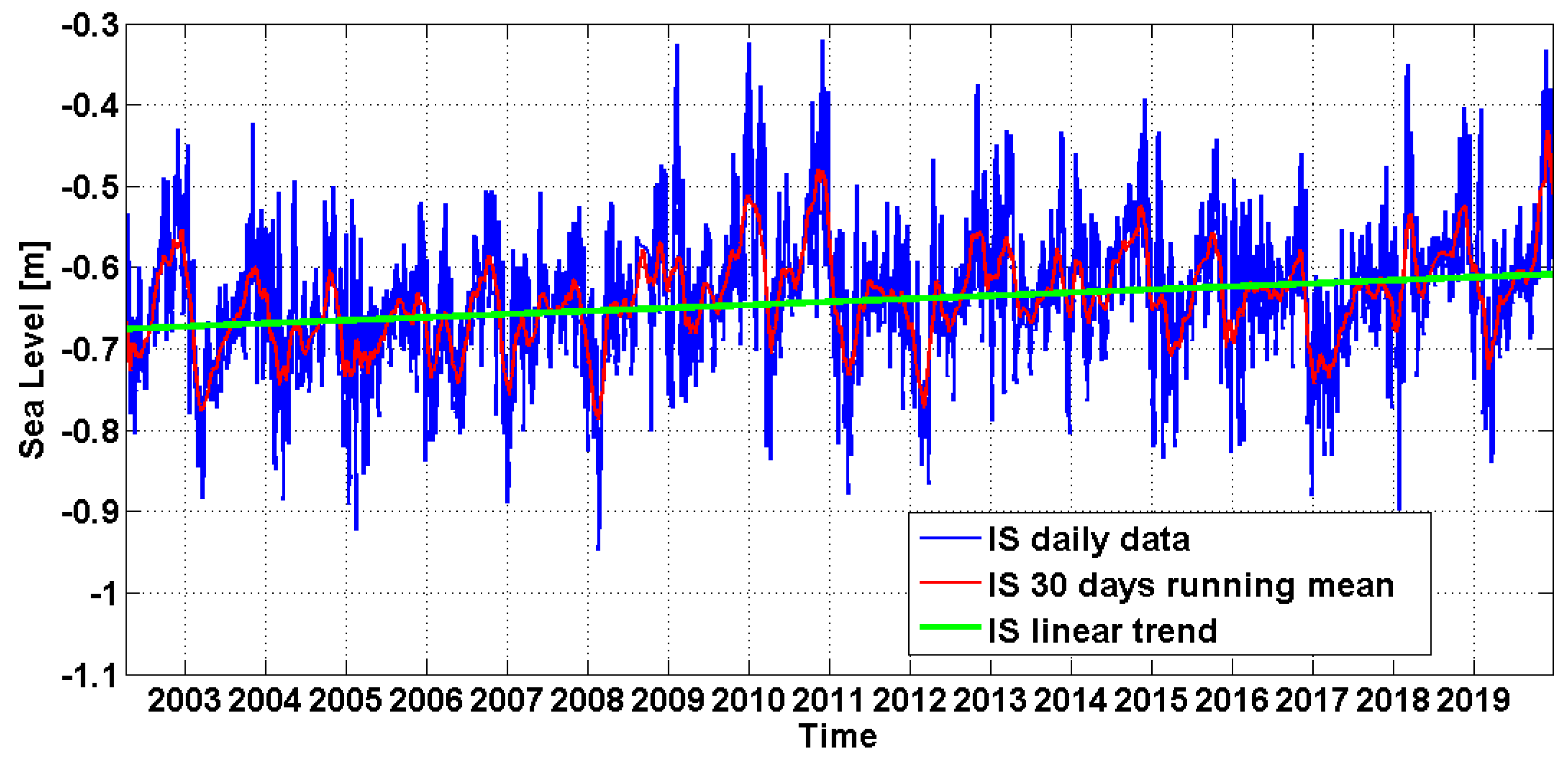
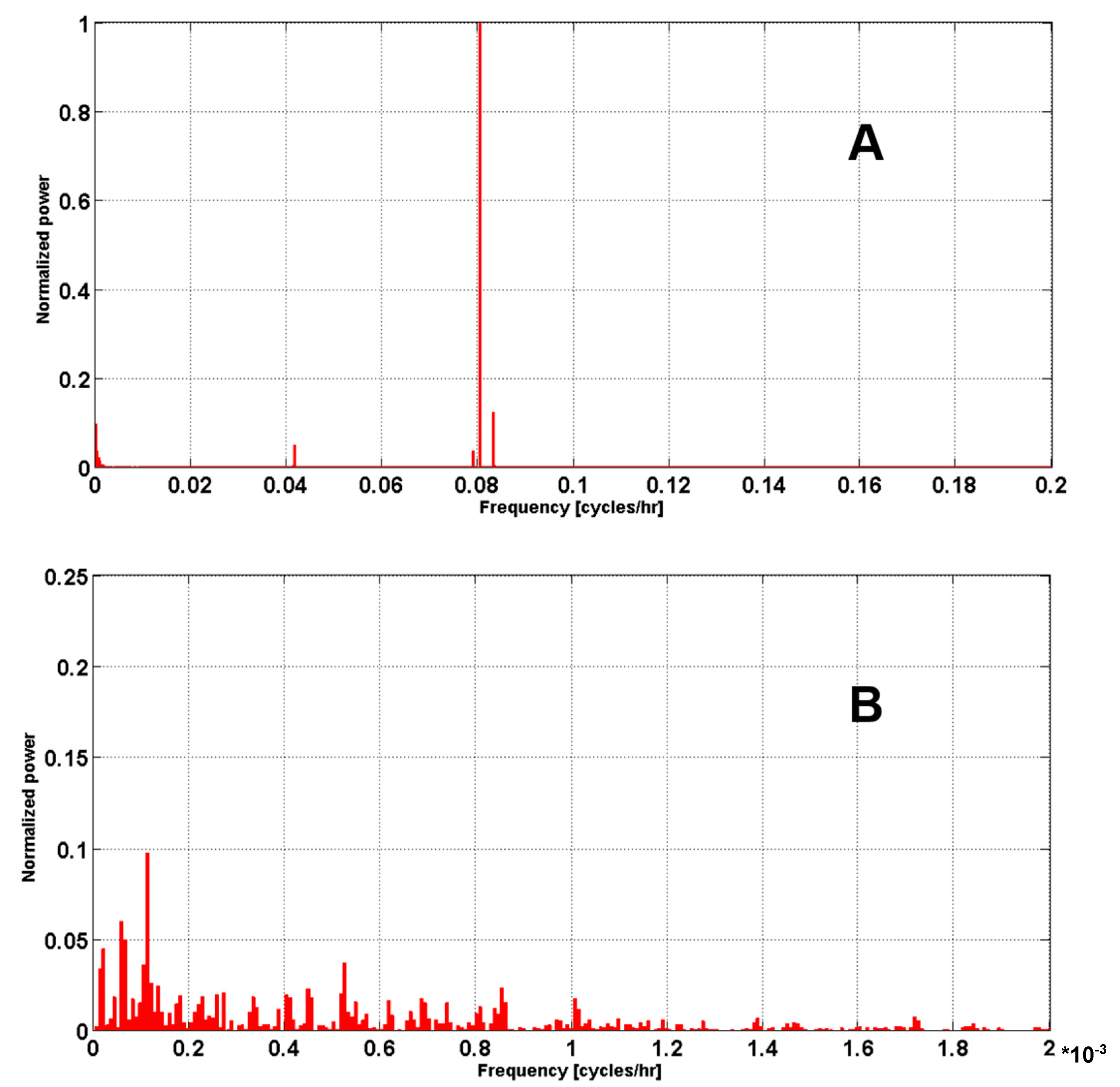
3.1. Tide-Gauge Data Preliminary Analysis and Tidal Constituents

The IS tide-gauge began operating on 26 March 2002. After quality control procedures were completed, its observations were analyzed in order to compute the “length”, “completeness”, and “continuity” of the 18 year time series (Figure 2). IS tide-gauge records were characterized by values of L = 18; Cy = 0.967, and Co = 0.983. This preliminary analysis was also carried out on the shorter (8 years) CS time series starting on 9 February 2011. The CS dataset was characterized by values of L = 8, Cy = 1, and Co = 1.
The IS tide-gauge data were used to calculate the tidal constants and estimate the power spectral density (PSD) of the IS timeseries. The calculation of tidal constants is particularly useful to analyze the tide at regional and local scales and to gain insight into their relationships with the dynamics of the basin. Furthermore, as satellite altimetry data are continuously improving their ability to investigate coastal areas, the tidal constants, and tide-gauge-data in IS could provide an important reference for remotely sensed data analysis and instrumental calibration [9,10,11,12,78].
In this work, the harmonic analysis of tides was carried out with the MATLAB “t-tide” tool [79]. Only tidal components with a signal to noise ratio of larger than 1 are reported (Table 1 and Table 2). Thanks to the 18-year-long timeseries of data, the IS tide-gauge makes an important contribution to the determination of tidal constants in the GON and offers well-established average values for the SL. Such a long time series—154,350 records, corresponding to about 6490 days of continuous data collection—allowed the calculation of the first 53 components of the astronomic tide at this site (Table 1).
To complement these results, a harmonic analysis of tide constituents was also carried out on the CS shorter tide-gauge dataset. The results from this site allowed us to estimate the tidal constants for 40 components to determine the astronomical tidal variability (Table 2).
Both the IS and CS values are in agreement with the estimations of the tidal constants based on data collected in Naples since 1986 by the Italian national tidal observation network (RMN—Rete Mareografica Nazionale) [80]. These results show that GON is characterized by the absence of any amphidromic system, with synchronous SL oscillation over the entire gulf. The regional dynamics are included in the larger spatial dynamics of the Tyrrhenian Sea that are characterized by synchronous variation in the SL over the entire basin [81]. According to the general Mediterranean circulation, the Tyrrhenian Sea is indeed characterized by a general cyclonic circulation along the boundaries and the presence of several quasi-permanent and intermittent cyclonic and anticyclonic structures across the basin, e.g., the strong and recurrent anticyclonic circulation that persists offshore of the GON [30]. The southern sector is also influenced by the recirculation processes occurring at its meridional openings, which are mainly driven by steric level gradients existing between this region and the adjacent basins.
The PSD analysis on IS data (Figure 3) shows, as expected, energy peaks corresponding to 12 and 24 h tidal cycles. Nevertheless, the length of the IS timeseries allows the determination of energy peaks at lower frequencies. The longest period observed in the IS data is 8 × 10⁻⁶ cycles per hour, corresponding to about 14.2 years. Similar results were achieved for CS (not shown), but the limited duration of this time series discouraged additional in-depth analysis of the CS dataset.
A PSD analysis on the mean sea level pressure data was also performed to evaluate the contribution of the meteorological variability to the computed power spectrum. The results show the presence of an energy peak at about 0.08 cycles per hour (Figure 4), which is probably due to the effects of the breeze regime on the tide gauge-site. However, most of the energy was found across longer time scales and was possibly associated with seasonal and interannual variations.

3.2. Trend Analysis

The IS area is characterized by seismic and volcanic phenomena affecting the ground elevation that cannot be ignored. In particular, low-intensity shallow seismicity, bradyseism activity, and intense hydrothermalism are active phenomena on the island [82]. The in situ measurements made along the geodetic network of the island of Ischia clearly show persistent and significant subsidence with a larger magnitude in the central-southern and north-western sectors of the island with a movement of up to 10 mm/year [83,84]. Additionally, the island shows large heterogeneity in the vertical displacement values [85]. Based on differential synthetic aperture radar interferometry data, Manzo et al. [83] demonstrated that the vertical displacements do not have any significant uplift but only have stable and subsiding areas. Among these, the Ischia Porto area, where the tide-gauge is located, is characterized by a vertical displacement trend ranging from +1 to −1 mm per year in the period 1992–2003, just before the tide-gauge installation. Successively, an analysis of the GPS survey data collected from 1998 to 2010 showed the existence of an elevation trend estimated to be 2.3 ± 0.9 mm/year in the data of the GPS station next to the Ischia tide-gauge [86], refining a previous estimation of −2.1 ± 1.0 mm/year obtained by De Martino et al. [87]. These values are in agreement with the satellite estimation (−2.3 mm/year) for the period 2002–2011 provided by the Italian National Science Council, Institute for the electromagnetic monitoring of the environment (IREA-CNR) through the webpage http://webgis.irea.cnr.it/webgis.html. A possible contribution of bradyseism to the SL records of Ischia was already hypothesized in the early 1900s basing on tide-gauge data collected by Giulio Glabrovitz, director of the local Casamicciola Geodynamical Observatory. In particular, he observed a relative SL rise of 3.5 mm/year for the period 1890–1910 in the same location as the modern tide-gauge [88].
Even though tide-gauges measure the height of the sea surface relative to crustal reference points that may move with tectonic activity or local subsidence, they can provide venerable information on long-term regional and global relative SL variations. To achieve this aim, IB correction was applied to IS measurements, and relative SL trend values were estimated. Results achieved through the Mann–Kendall and Sen methods report a linear trend of +3.93 mm per year (99.9% significance level) over the 18-year study period, as shown in Figure 2. This value is in agreement with the global mean SL rise estimate of 3.20 (2.80 to 3.60) mm per year found by different altimetry data processing groups for the period 1993–2012 [20], even though it was not possible to remove any eventual signals associated with vertical ground movement from the IS tide gauge data. Trend values calculated from relative SL data in this work are also consistent with trend values from 1993 to 2012 estimated by Bonaduce et al. [89] over the Mediterranean Sea on the basis of tide-gauge (3.50 ± 0.7 mm per year) and satellite data (2.64 ± 0.6 mm per year). Their analysis suggested the importance of events from 2010 to 2011 on the SL trend results.

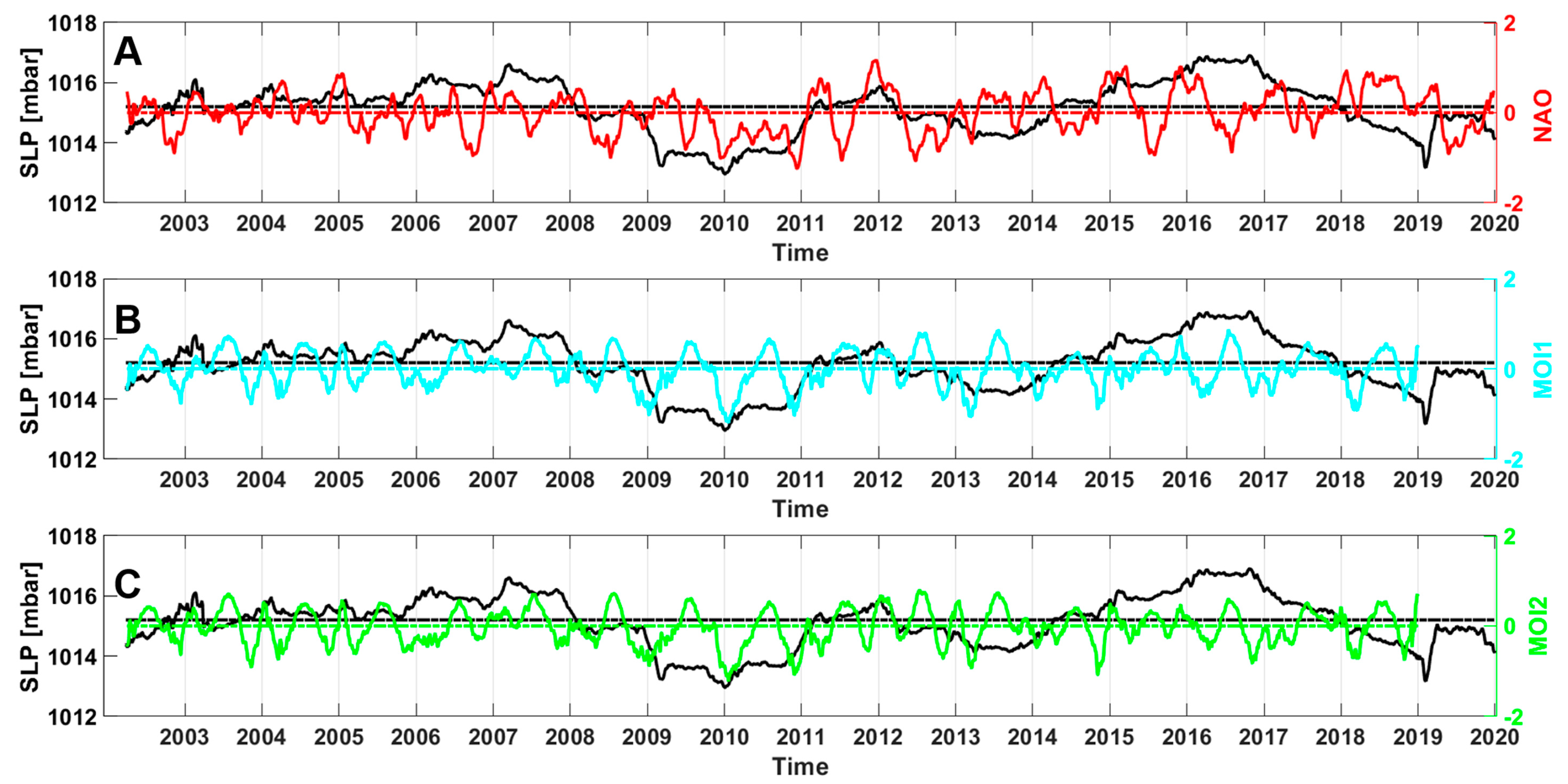
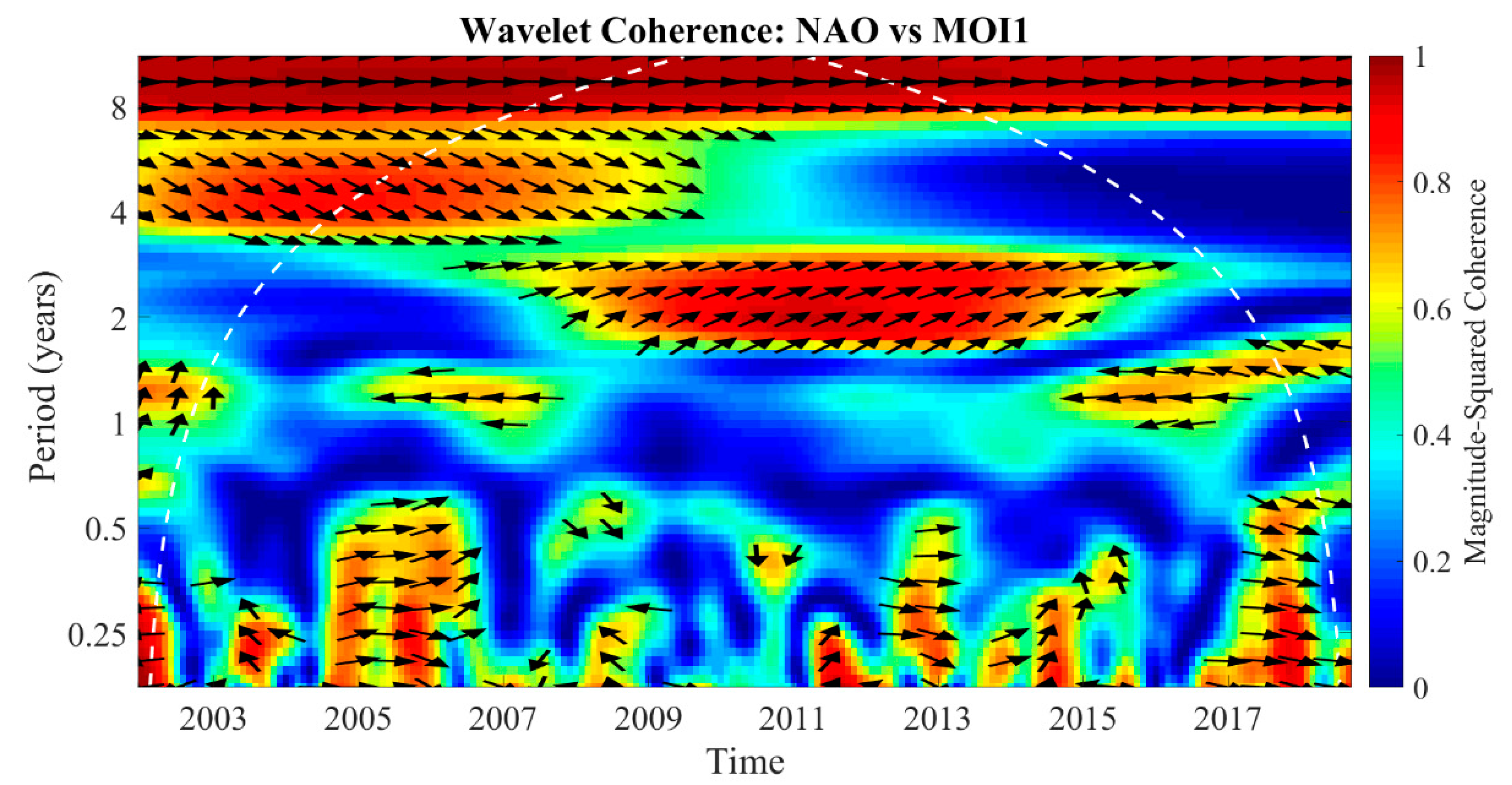
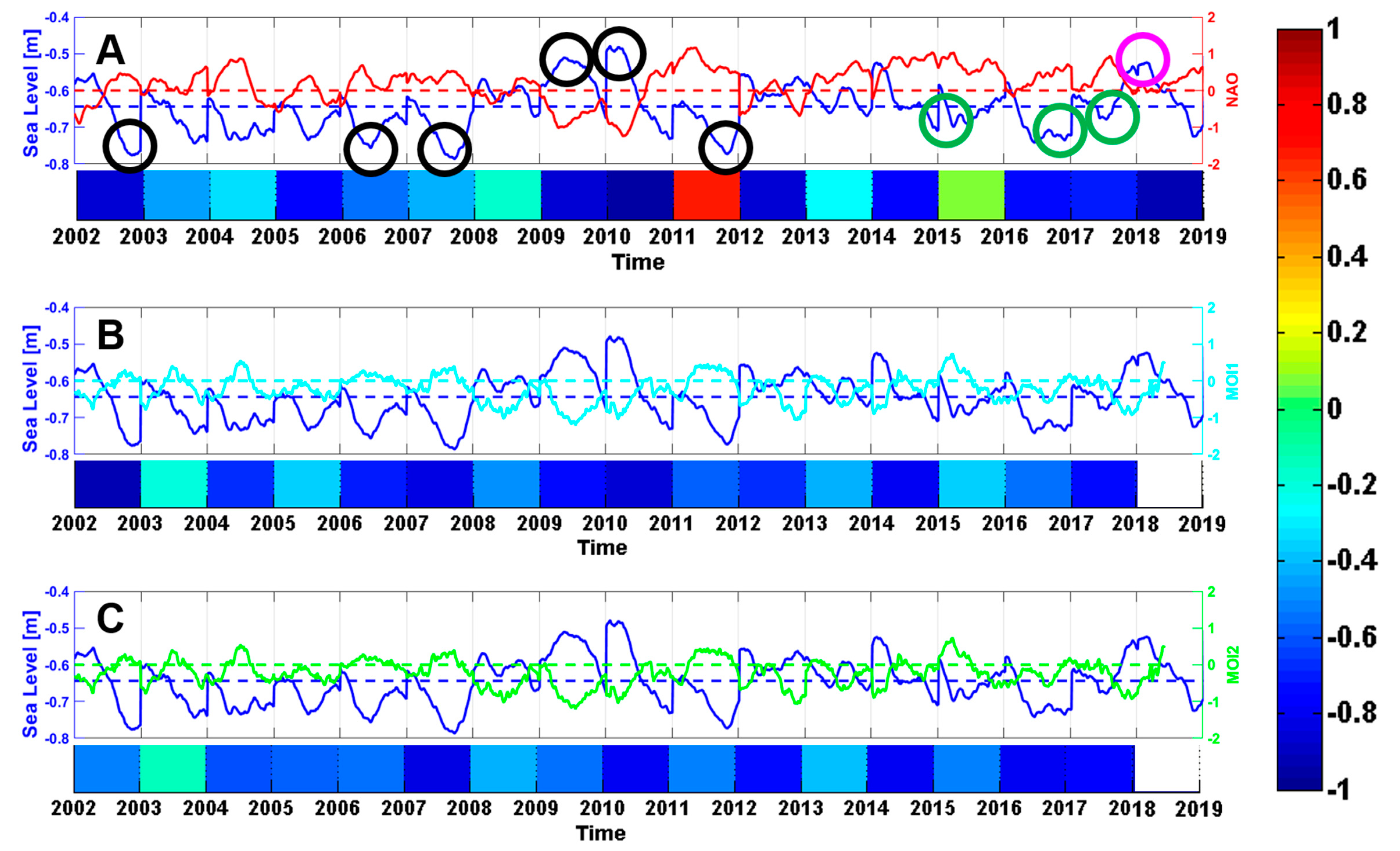
3.3. Relationship with Large-Scale Atmospheric Patterns

Air pressure variability has a direct effect on the SL variability on a wide range of time scales, from hourly to seasonal and multi-annual. For this reason, a detailed analysis of air pressure variability was carried out.
Figure 5 presents the behavior of atmospheric pressure data (black line) registered in Via Acton (January 2002–September 2011) and Centro Direzionale sites (October 2011–December 2019) over time and gives a comparison with NAO (red line), MOI1 (cyan line), and MOI2 (green line) indexes. A 30-day running mean was applied to the four signals in order to remove the very-high-frequency variability. According to the evidence presented in Figure 5, the period of interest (2002–2019) can be segmented into four different time intervals:
  • the 2002–2008 period, in which the air pressure is generally greater than its mean value;
  • the late-2008 to mid-2015 period, which is characterized by relevant oscillations of the atmospheric pressure signal; this interval includes two sub-periods in which negative air pressure anomalies prevailed: 2009–2011 and the segment encompassing late 2012 and early 2014;
  • the late 2015–2017 period, in which the air pressure is generally above its mean value;
  • 2018–2019, which is characterized by negative pressure anomalies.
As expected, the NAO and MOI indexes explain a large part of the observed variability, especially in the winter season. A monthly-based correlation analysis revealed that the first version of the MOI index (MOI1) is better suited to our study area than the second one (MOI2). More specifically, a clear linkage between MOI1 index and air pressure observed in Naples was found between December and March, with correlation values ranging from 0.5 to 0.7. The NAO index effectively modulates the meteorological features of the study area only in late autumn and early winter (November and December). The selected teleconnection patterns determined from sea-level pressure anomalies (see Section 2.2) are not adequate to capture the summer variability, e.g., [90,91]. The meteorological dynamics of this season, in fact, are generally driven by synoptic transients that are well structured only in the mid and upper tropospheric levels (i.e., cut-off lows and upper-level lows).
For each year, the annual means and standard deviations of the atmospheric pressure data were computed. The results are presented in Table 3. The percentages of samples with pressure levels higher than 1013 and 1026 mbar as well as those lower than 1013 and 1000 mbar are also reported. The value of 1013 mbar was chosen as the globally accepted boundary value between low- and high-pressure conditions, while two additional threshold values were chosen to represent the anomalous high (1026 mbar) and low (1000 mbar) pressure periods for the study area.
A close inspection of Table 3 highlights that in 2009, 2010, and 2013, the number of high-pressure samples was lower than in the other years and that the very-low-pressure records (≈4.5% < 1000 mbar) occurred about three times more often than in other years. On the other hand, during 2015, a relevant number of high-pressure events has been detected (13.7% > 1026 mbar). The footprint of large-scale atmospheric patterns on the strong variability and oscillations found between 2009 and 2015 is evident from Figure 5. This result was confirmed by Wavelet coherence (WC) analysis, a very useful tool that allows time-localized oscillations in non-stationary signals, such as geophysical signals, to be detected [92]. The WC shows that the NAO and MOI1 indexes exhibit common features between 2009 and 2015 with relatively low frequencies (between 2 and 4 years). According to the direction of the black arrows, the two signals are in phase, although NAO lags MOI by a phase angle of about 45° (Figure 6). Moreover, the WC spectrum highlights small areas of strong covariance in the high-frequency region (between 0.25 and 0.5 years) in 2005–2006, 2011–2013, and 2017–2018.
The WC analysis suggests that from 2009 to early 2011, as well as between late 2012 and early 2013, the persistence of both NAO and the MOI1 negative phase caused frequent low-pressure conditions on the central Mediterranean basin [93]. These anomalies in atmospheric pressure patterns may have a strong influence on SL variability, as is discussed in the next section.
To evaluate any correlation with the atmospheric variability as described by large-scale climate indices (i.e., NAO, MOI1, and MOI2), the meteorological tide time series for the IS tide-gauge was obtained by removing the astronomic theoretical tide from the signal. Hourly tidal constants obtained directly by harmonic analysis based on seven standard main constituents were used to obtain a new time series that still includes the IB component of the SL variations.
To examine the connections between the IS meteorological tide series and the teleconnection patterns, we focused on the period from November to March, which can be defined as an extended winter season. This choice is justified by the relevant linkages between the meteorological features of the study area and the synoptic variability only in late autumn, winter, and early spring, as previously shown. The results show that a moderate to strong anticorrelation exists on the long timescale between IS tide-gauge data and climate indices during the 2002–2019 study period, with the linear correlation coefficients being R = −0.5, R = −0.7, and R = −0.5 for NAO, MOI1, and MOI2, respectively.
The relationship between the two teleconnection patterns selected in this study, NAO and MOI, was further analyzed through a windowed correlation analysis. In particular, we estimated the correlation between the 30-day running mean of SL and the three teleconnection patterns for each extended winter season (November to March) for the period 2002–2019 (Figure 7).
An anti-phase relationship exists between MOIs and SL variability (Figure 7), as shown by the linear correlation coefficient that generally ranges from −0.4 to −0.8. However, there are some exceptions, i.e., during winter in 2003/2004, 2005/2006, and 2015/2016. In these years, a very weak correlation was found, especially when MOI1 index was considered. The Mediterranean atmospheric circulation had a very strong impact on SL in the following winter seasons: 2002/2003, 2006/2007, 2007/2008, 2009/2010, 2010/2011, 2014/2015, 2016/2017, and 2017/2018. It is not a mere coincidence that, in these cases, the NAO index (Figure 7, upper panel) also exhibited a moderate to strong anticorrelation with SL variability. A deeper examination of these seasons revealed some interesting linkages between atmospheric and mareographic variability, as discussed below.
During the first five winter seasons (2002/2003, 2006/2007, 2007/2008, 2009/2010, and 2010/2011) relevant anomalies of SL were observed (i.e., negative in 2002/2003, 2006/2007, and 2007/2008, positive in 2009/2010 and 2010/2011). Such events, marked as a black circle on the upper panel of Figure 7, were forced by a coupling between teleconnection patterns synthetized by the NAO and MOI. During these seasons, the indexes had quite similar behavior, i.e., a shift from a negative to a positive phase in 2002/2003, 2006/2007, and 2010/2011, persistence of the positive phase in 2007/2008, and a shift to a negative phase in 2009/2010. In 2002/2003, 2006/2007, and 2007/2008, the positive phase of both NAO and MOI resulted in a strong anticyclonic pattern over the central and western Mediterranean basins, which led to conditions favorable for a lowering of SL. Conversely, in the 2009/2010 and 2010/2011 seasons, the opposite large-scale circulation anomalies prevailed and the conditions were in favor of an increase in the SL in Ischia. Analogous results were achieved by Landerer and Volkov [93] who focused on recent SL variability in the Mediterranean Sea and found an increase in the mean SL of 10 cm during the boreal winter months of 2009/2010 and 2010/2011. Our findings reinforce their observations, including the assessment of a prominent role of the NAO on the observed SL fluctuations.
During the 2014/2015, 2016/2017, and 2017/2018 seasons, the NAO index was generally in its positive phase, while MOI1 and MOI 2 were neutral or negative. Despite the positive NAO phase having a magnitude comparable with that observed in the last part of 2002/2003, in the 2006/2007 and 2007/2008 seasons, its impact on Ischia SL was less relevant (Figure 7, green circles) due to a missing coupling with the Mediterranean atmospheric variability.
A strong lowering of SL, again marked by a black circle, also occurred in the extended winter season of 2011/2012. It is reasonable to assume that the positive phases of NAO and MOI strongly contributed to the relevant magnitude of the negative SL anomaly. Although in this season, the NAO index exhibited a negative trend, it remained in the positive phase, contributing, together with the positive phase of MOI, to a progressive regression of SL, culminating in January 2012. However, in this case, a positive linear correlation was found between NAO and SL. Available information cannot ensure that this result is ascribed to a mathematical artifact rather than a physical mechanism.
Finally, an interesting but isolated case is the rise of SL observed at the beginning of the 2018/2019 season (see magenta circle on the upper panel of Figure 7). Differently from the ones that occurred in 2009/2010 and in 2010/2011, this event was associated with a neutral NAO phase and a slightly negative MOI.

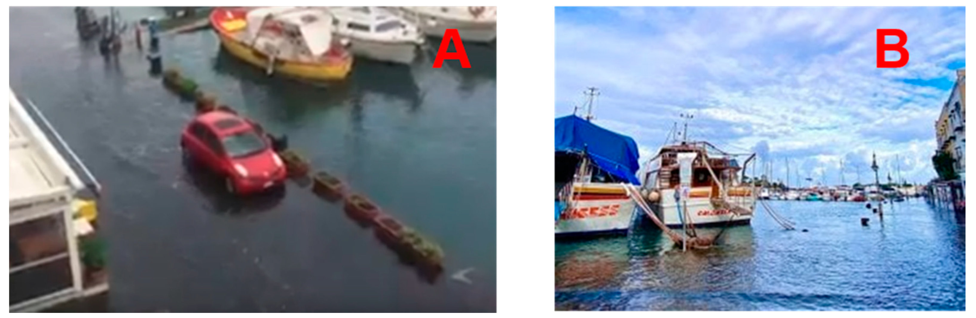
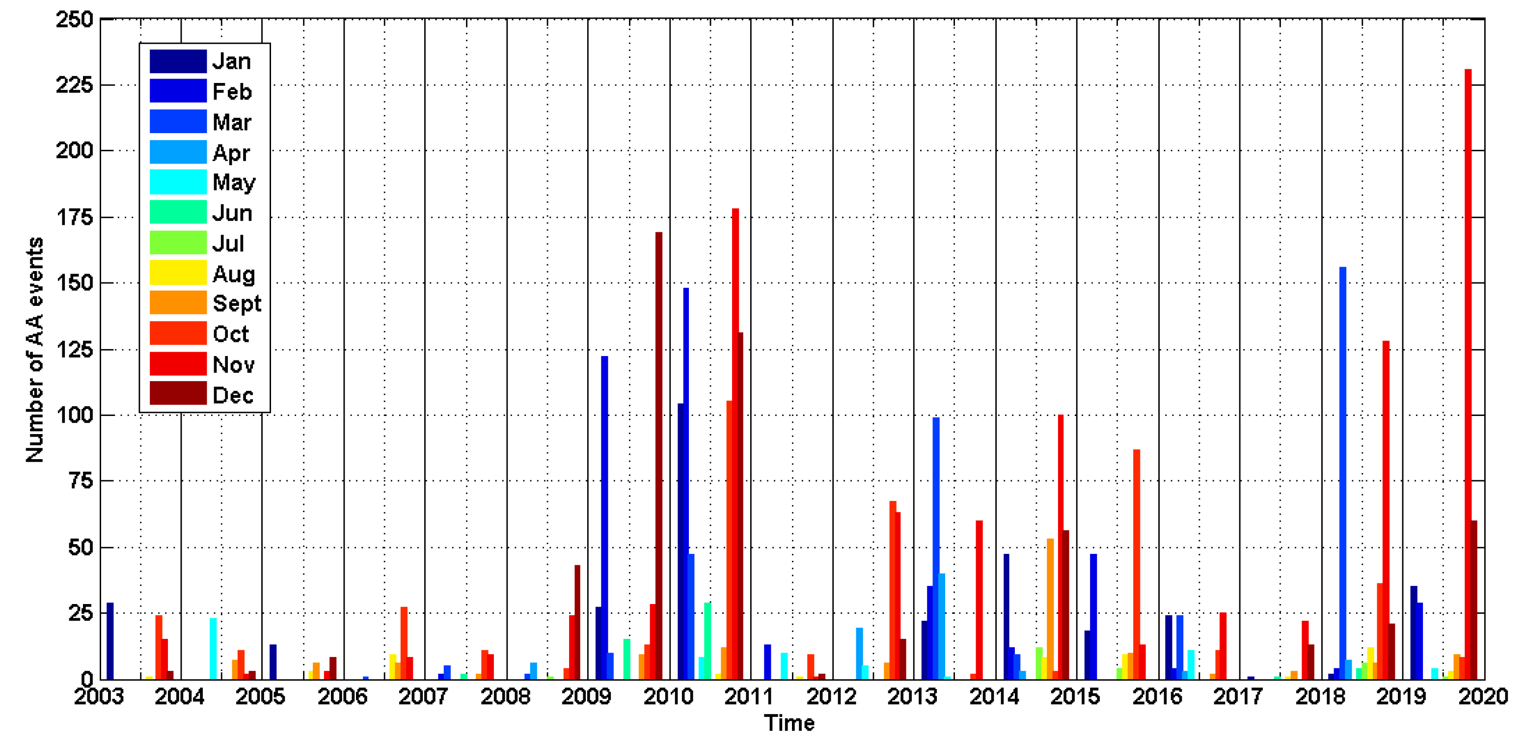
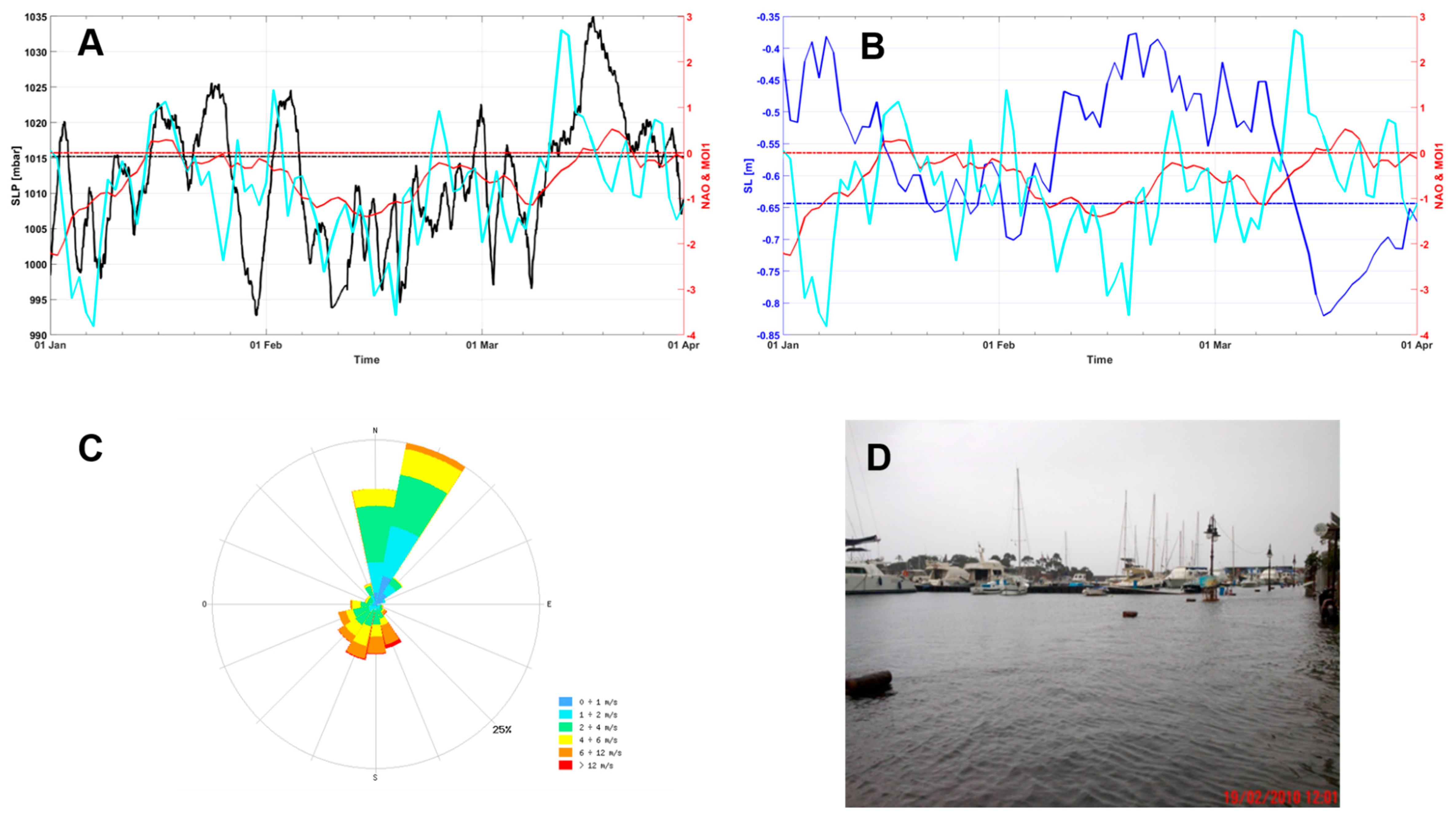
3.4. “Acqua Alta” Episodes in Ischia

SL variability is the result of several forces that act at different spatial and temporal scales and can be associated with changes in sea water properties, the so-called steric component, or not. In the Mediterranean Sea, at time scales longer than the seasonal scale, SL changes are due to both steric and non-steric forcing [42], while on a shorter timescale, the variability is mainly due to non-steric factors [93,94]. Among these, the combined effects of the wind air pressure and tides can result in the rapid submersion of coastal areas, leading to catastrophic flooding and danger to life and economic activities. This phenomenon is known as “acqua alta”, and it affects some Mediterranean areas, such as the city of Venice in the Northern Adriatic Sea and the island of Lipari in the Southern Tyrrhenian Sea.
In Ischia, AA events cause water ingression over the piers in the Ischia Porto area (Figure 8) and over the roads in the Ischia Ponte neighborhood, where intense socio-economic activities, mainly linked to tourism, exist. This phenomenon has gained the attention of the wider public in recent years, and its effects have been reported in a number of national and local newspapers.
In this work, the number, amplitude, and seasonal distribution of the AA events in Ischia Porto were studied (Table 4) through SL data collected by the IS tide-gauge since 2002. As described in Section 2, the IS tide-gauge is installed on the edge of the Coast Guard piers in the harbor that are 34 cm higher than the ancient piers limiting the “riva destra” area, where AA is more frequent. For this analysis, the edge of the Coast Guard pier was chosen as a reference. Hourly mean SL values overpassing the height of the old pier edge were considered to be single AA episodes. This analysis was performed on the original quality controlled timeseries recorded by the tide-gauge, in order to analyze the combined effects of tide and meteorological variability on the AA occurrences. Hourly means were used in order to minimize the effect of waves induced by ship movements or wind gusts as well as transient values that could influence the tide-gauge data during these events. For each year from 2002 to 2019, the total number of AA events is expressed as the percentage over the total number of hourly records. Table 4 also shows the number of events overpassing heights of 5, 10, 20, and 30 cm over the pier edge thresholds. After 2009, the AA episodes seem to have been more frequent, with only the years 2011 and 2017 having a percentage of single events lower than 1%. A higher number of AA episodes was registered in 2010 (8.7%), corresponding to about 762 submersion hours. During that year, the higher SL height over the pier was registered (32 cm) on October 1 at 09:00.
A similar analysis was carried out on a monthly basis in order to highlight the presence of a seasonal component in the AA occurrences. Figure 9 shows the monthly distribution of AA events from 2002 to 2019. The late fall and winter months from October to January were found to be characterized by an higher number of AA episodes, while during the spring and summer months, AA barely reached 30 episodes (June 2010).
Even though the estimated long-term SL rise has an effect on the frequency of the AA episodes through the expected increase in the mean SL, it cannot explain this phenomenon and its seasonal variability. Instead, the change in the frequency of AA events after 2009 may have been strongly influenced by large-scale atmospheric patterns. A detailed comparison between the results presented in Table 4 and Figure 9 and those reported in Table 1 and Figure 7 suggests that a relationship exists between the variability and fluctuations in atmospheric and AA events during the 2008–2015 interval.
A significant contribution could then be ascribed to the combined effect of low-pressure systems and wind forcing on the sea surface that generates so-called storm surges. To confirm this hypothesis, IS tide-gauge measurements and Via Acton air pressure data were complemented with wind direction and intensity data from 1 January 2010 to 31 March 2010 collected at the ISPRA weather station site in Naples. The analysis of the atmospheric variability during these three months shows that the large scale and Mediterranean circulation were conditioned by negative phases for both NAO and MOI1, especially in the first days of January and in the first twenty days of February (Figure 10a,b). The precondition for a storm surge event, i.e., a coupling between the two atmospheric teleconnections involved in our study, is recognizable in mid-February, when the atmospheric asset designed by negative phases of NAO and MOI caused negative pressure anomalies over the GON (Figure 10a), creating favorable conditions for an increase in SL (Figure 10b). Additionally, during those days, the wind regime over the GON was characterized by high-frequency winds from the N/NE that were able to directly impact on the Ischia harbor whose entrance is oriented toward North (Figure 10c). The effects of this atmospheric variability, associated with tidal SL variations, generated a significant storm surge event, as registered on 19 February (Figure 10d).
Therefore, the performed analyses suggest that the occurrence of AA events is the result of different degrees of forcing on the SL variability of Ischia, more so than the effects of tides or global SL rise. While SL rise can obviously contribute to setting a long-term situation that supports AA events, in situ tide-gauge data reveal that neither the number of AA events, nor the marked seasonal signals observed in their occurrence, are directly correlated with the SL trend. On the other hand, an increase in Ischia AA events is clearly associated with the NAO negative phases in conjunction with the low atmospheric pressure systems and wind patterns in the GON and over the Southern Tyrrhenian Sea. The combination of these forces should be considered as one leading factor fostering AA episodes.

4. Conclusions and Future Perspectives

The exploitation of IS tide-gauge data allowed the analysis of several aspects associated with SL variability in the Campania coastal area. The IS tidal constituents, corroborated by the analysis of the shorter CS time series, confirmed that the GON is characterized by non-amphidromic properties. Long-term trend analysis on the IS dataset showed a relative SL rise of 3.9 mm/year, in agreement with previous studies that focused on the Mediterranean Sea and the global mean SL rise.
The tidal variability and the global SL rise can explain a minor part of the SL variability measured by the IS tide-gauge, while the registered increasing occurrence of extreme events over the island, i.e., “acqua alta”, can be better described by a combination of factors. Firstly, an antiphase relationship was found between SL and two teleconnections that effectively describe the large-scale atmospheric variability and its anomalies, i.e., NAO and MOI. The latter modulates the tidal variability of the study area through the well-known IB effect in late fall, winter, and early spring, the months where most relevant SL anomalies have been detected. According to the results of our analysis, the main positive departures from the average SL, such as those observed in the 2009/2010 and 2010/2011 winter seasons, occurred when both NAO and MOI were simultaneously in their negative phase, which implies that there were low-pressure conditions in the central Mediterranean basin. At the same time, the strong SL lowering registered in the 2002/2003, 2006/2007, and 2007/2008 seasons can be explained by the coupling of NAO and MOI positive phases, which implies that there were anticyclonic conditions in the central and western Mediterranean area.
As demonstrated by the discussion of the AA event of February 2010, the storm surge dynamics are characterized by the combination of atmospheric forcing with the shape and morphology of Ischia harbor, which is most affected by the northern wind regime.
Of course, these results might improve as the tide-gauge time series becomes longer, so the accurate and regular maintenance of both IS and CS will be continued by the University “Parthenope” through planning and realizing the necessary operations during the forthcoming years.
Future developments are also expected, and these include the possibility of installing GPS and weather stations corresponding to the IS and CS tide-gauges, as recommended by international organizations and programs to discriminate between the effects of ground vertical movement and storms on SL variations. Additional analyses on long-term time series from different tide-gauges located in the Campania region and the Southern Tyrrhenian Sea are also advisable, as well as the opportunity to implement efficient procedures for comparing these data with available (and forthcoming) SL satellite observations.

Author Contributions

Conceptualization, B.B. and Y.C.; methodology, B.B., Y.C., V.C.; software, B.B. and G.Z.; validation, formal analysis, B.B., G.Z., V.C. and Y.C.; investigation, B.B., Y.C., V.C., G.A. and G.B.; writing—original draft preparation, B.B., Y.C., V.C., G.A.; writing—review and editing, G.A., G.B.; funding acquisition, G.B. All authors have read and agreed to the published version of the manuscript.

Funding

This research received no external funding.

Acknowledgments

The authors want to thank the Italian Air Force Weather Service for providing the air pressure data. We also thank the technicians working at the University of Naples “Parthenope” for their support on the design and maintenance of the tidal and meteorological network. The NAO daily timeseries used in this study was provided by the Climate Prediction Centre of the National Oceanic and Atmospheric Administration (NOAA). The MOI1 and MOI2 daily time series used in this study were provided by the University of East Anglia Climatic Research Unit. The authors thank the Marina di Stabia harbor management and the Corps of the Port Captaincies—Coast Guard of Ischia. We thank ISPRA for the wind data in Naples provided through the webpage https://www.mareografico.it/. Finally, the authors want to thank two anonymous reviewers for their work and the suggestions received. GA work was realized in the framework of the PON R&I 2014–2020 “AIM—Attraction and International Mobility” at Università degli Studi di Napoli Parthenope.

Conflicts of Interest

The authors declare no conflict of interest.

References

  1. Woodworth, P.L.; White, N.J.; Jevrejeva, S.; Holgate, S.J.; Church, J.A.; Gehrels, W.R. Evidence for the accelerations of sea level on multi-decade and century timescales. Int. J. Climatol. 2009, 29, 777–789. [Google Scholar] [CrossRef]
  2. Frederikse, T.; Riva, R.; Slobbe, C.; Broerse, T.; Verlaan, M. Estimating decadal variability in sea level from tide gauge records: An application to the North Sea. J. Geophys. Res. Oceans 2016, 121, 1529–1545. [Google Scholar] [CrossRef] [Green Version]
  3. Zerbini, S.; Raicich, F.; Prati, C.M.; Bruni, S.; Del Conte, S.; Errico, M.; Santi, E. Sea-level change in the Northern Mediterranean Sea from long-period tide-gauge time series. Earth Sci. Rev. 2017, 167, 72–87. [Google Scholar] [CrossRef]
  4. Ekman, M. The world’s longest continuous series of sea level observations. Pure Appl. Geophys. 1988, 127, 73–77. [Google Scholar] [CrossRef]
  5. Van Veen, J. Bestaat er een geologische bodemdaling te Amsterdam sedert 1700? Tijdschrift Koninklijk Nederlandsch Aardrijkskundig Genootschap. 1945. Available online: http://www.kwaad.net/VanVeen_1945_PeilAmsterdam_1700AD.pdf (accessed on 2 September 2020).
  6. Gornitz, V.; Lebedeff, S.; Hansen, J. Global sea level trend in the past century. Science 1982, 215, 1611–1614. [Google Scholar] [CrossRef] [PubMed]
  7. Douglas, B.C. Global sea level rise. J. Geophys. Res. 1991, 96, 6981–6992. [Google Scholar] [CrossRef] [Green Version]
  8. Higginson, S.; Thompson, K.R.; Woodworth, P.L.; Hughes, C.W. The tilt of mean sea level along the east coast of North America. Geophys. Res. Lett. 2015, 42, 1471–1479. [Google Scholar] [CrossRef] [Green Version]
  9. Passaro, M.; Rose, S.K.; Andersen, O.B.; Boergens, E.; Calafat, F.M.; Dettmering, D.; Benveniste, J. ALES+: Adapting a homogenous ocean retracker for satellite altimetry to sea ice leads, coastal and inland waters. Remote Sens. Environ. 2018, 211, 456–471. [Google Scholar] [CrossRef] [Green Version]
  10. Volkov, D.L.; Pujol, M.I. Quality assessment of a satellite altimetry data product in the Nordic, Barents, and Kara seas. J. Geophys. Res. Oceans 2012, 117, C03025. [Google Scholar] [CrossRef] [Green Version]
  11. Chambers, D.P.; Ries, J.C.; Shum, C.K.; Tapley, B.D. On the use of tide gauges to determine altimeter drift. J. Geophys. Res. Oceans 1998, 103, 12885–12890. [Google Scholar] [CrossRef]
  12. Wunsch, C. Calibrating an altimeter: How many tide gauges is enough? J. Atmos. Ocean. Technol. 1986, 3, 746–754. [Google Scholar] [CrossRef] [Green Version]
  13. Ding, X.; Zheng, D.; Chen, Y.; Chao, J.; Li, Z. Sea level change in Hong Kong from tide gauge measurements of 1954–1999. J. Geod. 2001, 74, 683–689. [Google Scholar] [CrossRef]
  14. Houghton, L.G.; Meira Filho, L.G.; Callander, B.A. (Eds.) Climate Change 1995: The Science of Climate Change; Cambridge University Press: Cambridge, UK, 1996. [Google Scholar]
  15. Warrick, R.A.; Oerlemans, J.; Woodworth, P.L.; Meier, M.F.; le Provost, C. Changes in sea level. In Climate Change 1995: The Science of Climate Change; Houghton, J.T., Meira Filho, L.G., Callander, B.A., Eds.; Cambridge University Press: Cambridge, UK, 1996; pp. 359–405. [Google Scholar]
  16. Church, J.A.; Clark, P.U.; Cazenave, A.; Gregory, J.M.; Jevrejeva, S.; Levermann, A.; Merrifield, M.A.; Milne, G.A.; Nerem, R.S.; Nunn, P.D.; et al. Sea Level Change. In Climate Change 2013: The Physical Science Basis; Contribution of Working Group I to the Fifth Assessment Report of the Intergovernmental Panel on Climate Change; Stocker, T.F., Qin, D., Plattner, G.-K., Tignor, M., Allen, S.K., Boschung, J., Nauels, A., Xia, Y., Bex, V., Midgley, P.M., Eds.; Cambridge University Press: Cambridge, UK; New York, NY, USA, 2013; pp. 1137–1216. [Google Scholar]
  17. Nerem, R.S.; Beckley, B.D.; Fasullo, J.T.; Hamlington, B.D.; Masters, D.; Mitchum, G.T. Climate-change-driven accelerated sea-level rise detected in the altimeter era. Proc. Natl. Acad. Sci. USA 2018, 115, 2022–2025. [Google Scholar] [CrossRef] [PubMed] [Green Version]
  18. Mahdi, H.; Hebib, T. Mediterranean Sea level trends from long-period tide gauge time series. Acta Oceanol. Sin. 2020, 39, 157–165. [Google Scholar] [CrossRef]
  19. Intergovernmental Panel on Climate Change (IPCC). Climate Change 2013: The Physical Science Basis; 2013. Available online: http://www.climatechange2013.org (accessed on 17 July 2018).
  20. Intergovernmental Panel on Climate Change (IPCC). Climate Change 2014: Synthesis Report. Contribution of Working Groups I, II and III to the Fifth Assessment Report of the Intergovernmental Panel on Climate Change; Core Writing Team, Pachauri, R.K., Meyer, L.A., Eds.; IPCC: Geneva, Switzerland, 2014; p. 151. [Google Scholar]
  21. Bruni, S.; Zerbini, S.; Raicich, F.; Errico, M. Rescue of the 1873–1922 high and low waters of the Porto Corsini/Marina di Ravenna (northern Adriatic, Italy) tide gauge. J. Geod. 2019, 93, 1227–1244. [Google Scholar] [CrossRef]
  22. Tsimplis, M.N.; Baker, T.F. Sea level drop in the Mediterranean Sea: An indicator of deep water salinity and temperature changes? Geophys. Res. Lett. 2000, 27, 1731–1734. [Google Scholar] [CrossRef]
  23. Cazenave, A.; Cabanes, C.; Dominh, K.; Mangiarotti, S. Recent sea level changes in the Mediterranean Sea revealed by TOPEX/POSEIDON satellite altimetry. Geophys. Res. Lett. 2001, 28, 1607–1610. [Google Scholar] [CrossRef]
  24. Fenoglio-Marc, L. Analysis and representation of regional sealevel variability from altimetry and atmospheric-oceanic data. Geophys. J. Int. 2001, 145, 1–18. [Google Scholar] [CrossRef]
  25. Antonioli, F.; Silenzi, S. Variazioni Relative del Livello del Mare e Vulnerabilita Delle Pianure Costiere Italiane. Quaderno della Soc. Geol. Ital. 2007, 2, 1–29. [Google Scholar]
  26. Lambeck, K.; Antonioli, F.; Anzidei, M.; Ferranti, L.; Leoni, G.; Scicchitano, G.; Silenzi, S. Sea level change along the Italian coast during the Holocene and projections for the future. Quatern. Int. 2011, 232, 250–257. [Google Scholar] [CrossRef]
  27. Aucelli, P.C.; Di Paola, G.; Incontri, P.; Rizzo, A.; Vilardo, G.; Benassai, G.; Buonocore, B.; Pappone, G. Coastal inundation risk assessment due to subsidence and sea level rise in a Mediterranean alluvial plain (Volturno coastal plain–southern Italy). Estuar. Coast. Shelf Sci. 2016. [Google Scholar] [CrossRef]
  28. Thompson, P.R.; Hamlington, B.D.; Landerer, F.W.; Adhikari, S. Are long tide gauge records in the wrong place to measure global mean sea level rise? Geophys. Res. Lett. 2016, 43, 10403–10411. [Google Scholar] [CrossRef] [Green Version]
  29. Dangendorf, S.; Hay, C.C.; Calafat, F.M.; Marcos, M.; Berk, K.; Jensen, J. Persistent acceleration in global sea-level rise since the 1970s. Nat. Clim. Chang. 2019, 9, 705–710. [Google Scholar] [CrossRef] [Green Version]
  30. Aulicino, G.; Cotroneo, Y.; Lacava, T.; Sileo, G.; Fusco, G.; Carlon, R.; Satriano, V.; Pergola, N.; Tramutoli, V.; Budillon, G. Results of the first wave glider experiment in the southern Tyrrhenian Sea. Adv. Oceanogr. Limnol. 2016, 7, 16–35. [Google Scholar] [CrossRef] [Green Version]
  31. Durante, S.; Schroeder, K.; Mazzei, L.; Pierini, S.; Borghini, M.; Sparnocchia, S. Permanent thermohaline staircases in the Tyrrhenian Sea. Geophys. Res. Lett. 2019, 46, 1562–1570. [Google Scholar] [CrossRef] [Green Version]
  32. Castagno, P.; de Ruggiero, P.; Pierini, S.; Zambianchi, E.; De Alteris, A.; De Stefanoet, M.; Budillon, G. Hydrographic and dynamical characterization of the Bagnoli-Coroglio Bay (Gulf of Naples, Tyrrhenian Sea). Chem. Ecol. 2020. [Google Scholar] [CrossRef]
  33. ISPRA-CARG. Geological Map of Italy 1:50,000 Scale, Sheet 464 “Ischia”. 2009. Available online: https://www.isprambiente.gov.it/Media/carg/464_ISOLA_DISCHIA/Foglio.html (accessed on 5 August 2020).
  34. ISPRA-CARG. Geological Map of Italy 1:50,000 Scale, Sheet 466 “Castellammare”. 2009. Available online: https://www.isprambiente.gov.it/Media/carg/466_485_SORRENTO_TERMINI/Foglio.html (accessed on 5 August 2020).
  35. IOC. Manual on Sea Level Measurement and Interpretation: Volume I—Basic Procedures; IOC Manuals and Guides 14; UNESCO: Paris, France, 1985; p. 75. [Google Scholar]
  36. IOC. Manual on Sea Level Measurement and Interpretation: Volume II—Emerging Technologies; IOC Manuals and Guides 14; UNESCO: Paris, France, 1994; p. 52. [Google Scholar]
  37. IOC. Manual on Sea Level Measurement and Interpretation: Volume IV—An Update to 2006; IOC Manuals and Guides 14; UNESCO: Paris, France, 2006; p. 80. [Google Scholar]
  38. ISPRA. Manuale di Mareografia e Linee Guida per i Processi di Validazione dei Dati Mareografici; Manuali e Linee Guida; ISPRA: Rome, Italy, 2012; ISBN 978-88-448-0532-6. [Google Scholar]
  39. ISPRA. Linee Guida pe L’analisi e L’elaborazione Statistica di Base Delle Serie Storiche di Dati Idrologici; ISPRA: Rome, Italy, 2013. [Google Scholar]
  40. Pugh, D.T. Tides, Surges and Mean Sea-Level; John Wiley & Sons: New York, NY, USA, 1987. [Google Scholar]
  41. Doodson, A.T. The analysis of tidal observations. Philos. Trans. R. Soc. Lond. Ser. A Contain. Pap. Math. Phys. Character 1928, 227, 223–279. [Google Scholar]
  42. Woodworth, P.; Melet, A.; Marcos, M.; Ray, R.D.; Wöppelmann, G.; Sasaki, Y.N.; Cirano, M.; Hibbert, A.; Huthnance, J.M.; Monserrat, S.; et al. Forcing Factors Affecting Sea Level Changes at the Coast. Surv. Geophys. 2019, 40, 1351–1397. [Google Scholar] [CrossRef] [Green Version]
  43. Roden, G.I.; Rossby, H.T. Early Swedish contribution to oceanography: Nils Gissler (1715–1771) and the inverted barometer effect. Bull. Am. Meteorol. Soc. 1999, 80, 675–682. [Google Scholar] [CrossRef] [Green Version]
  44. Rogers, J.C. The association between the North Atlantic Oscillation and the Southern Oscillation in the Northern Hemisphere. Mon. Weather Rev. 1984, 112, 1999–2015. [Google Scholar] [CrossRef]
  45. Rogers, J.C. Atmospheric circulation changes associated with the warming over the northern North Atlantic in the 1920s. J. Clim. Appl. Meteorol. 1985, 24, 1303–1310. [Google Scholar] [CrossRef]
  46. Hurrel, J.W. Decadal Trends in the North Atlantic Oscillation: Regional Temperatures and Precipitation. Science 1995, 269, 676–679. [Google Scholar] [CrossRef] [PubMed] [Green Version]
  47. Rodwell, M.J.; Rowell, D.P.; Folland, C.K. Oceanic forcing of the wintertime North Atlantic Oscillation and European climate. Nature 1999, 398, 320–323. [Google Scholar] [CrossRef]
  48. Eshel, G.; Cane, M.A.; Farrell, B.F. Forecasting eastern Mediterranean droughts. Mon. Weather Rev. 2000, 128, 3618–3630. [Google Scholar] [CrossRef] [Green Version]
  49. Capozzi, V.; Budillon, G. Detection of heat and cold waves in Montevergine time series (1884–2015). Adv. Geosci. 2017, 44, 35–51. [Google Scholar] [CrossRef] [Green Version]
  50. Rezaeian, M.; Mohebalhojeh, A.R.; Ahmadi-Givi, F.; Nasr-Esfahany, M. A wave-activity view of the relation between the Mediterranean storm track and the North Atlantic Oscillation in winter. Q. J. R. Meteorol. Soc. 2016, 142, 1662–1671. [Google Scholar] [CrossRef]
  51. Hastenrath, S.; Greischar, L. The North Atlantic Oscillation in the NCEP-NCAR reanalysis. J. Clim. 2001, 14, 2404–2413. [Google Scholar] [CrossRef]
  52. Barnston, A.G.; Livezey, R.E. Classification, seasonality and persistence of low-frequency atmospheric circulation patterns. Mon. Weather Rev. 1987, 115, 1083–1126. [Google Scholar] [CrossRef]
  53. Han, W.; Stammer, D.; Thompson, P.; Ezer, T.; Palanisamy, H.; Zhang, X.; Domingues, C.; Zhang, L.; Yuan, D. Impacts of basin-scale climate modes on coastal sea level: A review. Surv. Geophys. 2019. [Google Scholar] [CrossRef] [PubMed] [Green Version]
  54. Tsimplis, M.N.; Shaw, A.G.P. The forcing of mean sea level variability around Europe. Glob. Planet. Chang. 2008, 63, 196–202. [Google Scholar] [CrossRef]
  55. Wakelin, S.L.; Woodworth, P.L.; Flather, R.A.; Williams, J.A. Sea-level dependence on the NAO over the NW European Continental Shelf. Geophys. Res. Lett. 2003, 30, 1403. [Google Scholar] [CrossRef]
  56. Woolf, D.K.; Shaw, A.G.P.; Tsimplis, M.N. The influence of the North Atlantic Oscillation on sea-level variability in the North Atlantic region. J. Atmos. Ocean. Sci. 2003, 9, 145–167. [Google Scholar] [CrossRef]
  57. Yan, Z.W.; Tsimplis, M.N.; Woolf, D. Analysis of the relationship between the North Atlantic oscillation and sea-level changes in northwest Europe. Int. J. Climatol. 2004, 24, 743–758. [Google Scholar] [CrossRef]
  58. Hughes, C.W.; Meredith, C.P. Coherent sea-level fluctuations along the global continental slope. Philos. Trans. R. Soc. A 2006, 364, 885–901. [Google Scholar] [CrossRef] [Green Version]
  59. Tsimplis, M.N.; Shaw, A.G.P.; Flather, R.A.; Woolf, D.K. The influence of the North Atlantic Oscillation on the sea-level around the northern European coasts reconsidered: The thermosteric effects. Philos. Trans. R. Soc. A 2006, 364, 845–856. [Google Scholar] [CrossRef]
  60. Miller, L.; Douglas, B.C. Gyre-scale atmospheric pressure variations and their relation to 19th and 20th century sea level rise. Geophys. Res. Lett. 2007, 34, L16602. [Google Scholar] [CrossRef]
  61. Gomis, D.; Ruiz, S.; Sotillo, M.G.; Alvarez-Fanjul, E.; Terradas, J. Low frequency Mediterranean Sea level variability: The contribution of atmospheric pressure and wind. Glob. Planet. Chang. 2008, 63, 215–229. [Google Scholar] [CrossRef]
  62. Calafat, F.M.; Chambers, D.P.; Tsimplis, M.N. Mechanisms of decadal sea level variability in the eastern North Atlantic and the Mediterranean Sea. J. Geophys. Res. Oceans 2012, 117, C09022. [Google Scholar] [CrossRef]
  63. Tsimplis, M.N.; Calafat, F.M.; Marcos, M.; Jorda, G.; Gomis, D.; Fenoglio-Marc, L.; Struglia, M.V.; Josey, S.A.; Chambers, D.P. The effect of the NAO on sea level and on mass changes in the Mediterranean Sea. J. Geophys. Res. Oceans 2013, 118, 944–952. [Google Scholar] [CrossRef] [Green Version]
  64. Dangendorf, S.; Calafat, F.M.; Arns, A.; Wahl, T.; Haigh, I.D.; Jensen, J. Mean sea level variability in the North Sea: Processes and implications. J. Geophys. Res. Oceans 2014, 119, 6820–6841. [Google Scholar] [CrossRef] [Green Version]
  65. Ezer, T.; Haigh, I.D.; Woodworth, P.L. Nonlinear sea-level trends and long-term variability on Western European coasts. J. Coast. Res. 2016, 32, 744–755. [Google Scholar] [CrossRef]
  66. Brunetti, M.; Maugeri, M.; Nanni, T. Atmospheric circulation and precipitation in Italy for the last 50 years. Int. J. Climatol. 2002, 22, 1455–1471. [Google Scholar] [CrossRef]
  67. Conte, M.; Giuffrida, A.; Tedesco, S. The Mediterranean Oscillation. Impact on Precipitation and Hydrology in Italy Climate Water; Publications of the Academy of Finland: Helsinki, Finland, 1989. [Google Scholar]
  68. Colacino, M.; Conte, M. Greenhouse effect and pressure patterns in the Mediterranean Basin. Il Nuovo Cimento C 1993, 16, 67–76. [Google Scholar] [CrossRef]
  69. Palutikof, J.P.; Conte, M.; Casimiro Mendes, J.; Goodess, C.M.; Espirito Santo, F. Climate and climate change. In Mediterranean Desertification and Land Use; Brandt, C.J., Thornes, J.B., Eds.; John Wiley and Sons: London, UK, 1996. [Google Scholar]
  70. Piervitali, E.; Colacino, M.; Conte, M. Rainfall over the central–western Mediterranean basin in the period 1951–1995. Part II: Precipitation scenarios. Il Nuovo Cimento C 1999, 22, 649–661. [Google Scholar]
  71. Palutikof, J.P. Analysis of Mediterranean climate data: Measured and modelled. In Mediterranean Climate: Variability and Trends; Bolle, H.J., Ed.; Springer: Berlin, Germany, 2003. [Google Scholar]
  72. Dietz, E.J.; Killeen, T.J. A Nonparametric Multivariate Test for Monotone Trend with Pharmaceutical Applications. J. Am. Stat. Assoc. 1981, 76, 169–174. [Google Scholar] [CrossRef]
  73. Gocic, M.; Trajkovic, S. Analysis of changes in meteorological variables using Mann–Kendall and Sen’s slop e estimator statistical tests in Serbia. Glob. Planet. Chang. 2013, 100, 172–182. [Google Scholar] [CrossRef]
  74. Fusco, G.; Artale, V.; Cotroneo, Y.; Sannino, G. Thermohaline variability of Mediterranean Water in the Gulf of Cádiz, 1948–1999. Deep-Sea Res. I 2008, 55, 1624–1638. [Google Scholar] [CrossRef]
  75. Mann, H.B. Nonparametric tests against trend. Econometrica 1945, 13, 245–259. [Google Scholar] [CrossRef]
  76. Kendall, M.G. Rank Correlation Methods; Griffin: London, UK, 1975. [Google Scholar]
  77. Sen, P.K. Estimates of the regression coefficient based on Kendall’s tau. J. Am. Stat. Assoc. 1968, 63, 1379–1389. [Google Scholar] [CrossRef]
  78. Piccioni, G.; Dettmering, D.; Bosch, W.; Seitz, F. TICON: TIdal CONstants based on GESLA sea-level records from globally located tide gauges. Geosci. Data J. 2019, 6, 97–104. [Google Scholar] [CrossRef] [Green Version]
  79. Pawlowicz, R.; Beardsley, R.; Lentz, S. Classical tidal harmonic analysis including error estimates in MATLAB using T_TIDE. Comput. Geosci. 2002, 28, 929–937. [Google Scholar] [CrossRef]
  80. Lama, R.; Corsini, S. Analisi dei dati Storici della Rete Mareografica Italiana; Ed. Poligrafico dello Stato: Rome, Italy, 2003. [Google Scholar]
  81. Mosetti, F.; Purga, N. Le maree del mar Tirreno. Boll. Oceanol. Teor. Appl. 1985, 3, 83–102. [Google Scholar]
  82. Rapolla, A.; Paoletti, V.; Secomandi, M. Seismically-induced landslide susceptibility evaluation: Application of a new procedure to the island of Ischia, Campania Region, Southern Italy. Eng. Geol. 2010, 114, 10–25. [Google Scholar] [CrossRef]
  83. Manzo, M.; Ricciardi, G.P.; Casu, F.; Ventura, G.; Zeni, G.; Borgstrom, S.; Berardino, P.; Del Gaudio, C.; Lanari, R. Surface deformation analysis in the Ischia Island (Italy) based on spaceborne radar interferometry. J. Volcanol. Geotherm. Res. 2006, 151, 399–416. [Google Scholar] [CrossRef]
  84. Sepe, V.; Atzori, S.; Ventura, G. Subsidence due to crack closure and depressurization of hydrothermal systems: A case study from Mt Epomeo (Ischia Island, Italy). Terra Nova 2007, 19, 127–132. [Google Scholar] [CrossRef]
  85. Ricco, C.; Petrosino, S.; Aquino, I.; Del Gaudio, C.; Falanga, M. Some Investigations on a Possible Relationship between Ground Deformation and Seismic Activity at Campi Flegrei and Ischia Volcanic Areas (Southern Italy). Geosciences 2019, 9, 222. [Google Scholar] [CrossRef] [Green Version]
  86. Cubellis, E.; Luongo, G.; Obrizzo, F.; Sepe, V.; Tammaro, U. Contribution to knowledge regarding the sources of earthquakes on the island of Ischia (Southern Italy). Nat. Hazards 2020, 100, 955–994. [Google Scholar] [CrossRef]
  87. De Martino, P.; Tammaro, U.; Obrizzo, F.; Sepe, V.; Brandi, G.; D’Alessandro, A.; Dolce, M.; Pingue, F. La rete GPS dell’isola d’Ischia: Deformazioni del suolo in un’area vulcanica attiva (1998–2010). In Quaderni di Geofisica INGV Roma; INGV Istituto Nazionale di Geofisica e Vulcanologia: Rome, Italy, 2011; ISSN 1590-2595-95:4-23; Available online: http://istituto.ingv.it/images/collane-editoriali/quaderni-di-geofisica/quaderni-di-geofisica-2011/quaderno95.pdf (accessed on 25 June 2020).
  88. Grablovitz, G. Il mareografo d’Ischia in relazione ai bradisismi. Boll. Della Soc. Sismol. Ital. 1911, 15, 144–153. [Google Scholar]
  89. Bonaduce, A.; Pinardi, N.; Oddo, P.; Spada, G.; Larnicol, G. Sea-level variability in the Mediterranean Sea from altimetry and tide gauges. Clim. Dyn. 2016, 1–16. [Google Scholar] [CrossRef] [Green Version]
  90. Milošević, D.D.; Savić, S.M.; Pantelić, M.; Stankov, U.; Žiberna, I.; Dolinaj, D.; Leščešen, I. Variability of seasonal and annual precipitation in Slovenia and its correlation with large-scale atmospheric circulation. Open Geosci. 2016, 8, 593–605. [Google Scholar] [CrossRef]
  91. Folland, C.K.; Knight, J.; Linderholm, H.W.; Fereday, D.; Ineson, S.; Hurrell, J.W. The summer North Atlantic Oscillation: Past, present, and future. J. Clim. 2009, 22, 1082–1103. [Google Scholar] [CrossRef]
  92. Grinsted, A.; Moore, J.C.; Jevrejeva, S. Application of the cross wavelet transform and wavelet coherence to geophysical time series. Nonlin. Process. Geophys. 2004, 11, 561–566. [Google Scholar] [CrossRef]
  93. Landerer, F.W.; Volkov, D.L. The anatomy of recent large sea level fluctuations in the Mediterranean Sea. Geophys. Res. Lett. 2013, 40. [Google Scholar] [CrossRef]
  94. Fukumori, I.; Menemenlis, D.; Lee, T. A near-uniform basinwide sea level fluctuation of the Mediterranean Sea. J. Phys. Oceanogr. 2007, 37, 338–358. [Google Scholar] [CrossRef] [Green Version]
Figure 1. Study area (upper panels) and locations of the Ischia (IS—red square) and Castellammare di Stabia (CS—green square) tide-gauges. Bathymetry is indicated through the color scale. The lower (left and right) panels show the IS and CS sites respectively.
Water 12 02466 g001
Figure 2. Daily tide-gauge data collected in Ischia from 2002 to 2019 (blue line). A 30-day running mean (red line) and a linear trend of the data (green line) are also shown.
Water 12 02466 g002
Figure 3. Normalized power spectrum of tide-gauge measurements in Ischia (A). The frequency is expressed in cycles per hour. Panel (B) offers a zoom-in view of the x-axis interval from 0 to 0.002 cycles/hr.
Water 12 02466 g003
Figure 4. Normalized power spectrum of atmospheric pressure measurements in Napoli. The frequency is expressed in cycles per hour.
Water 12 02466 g004
Figure 5. Time series of air pressure data (black line), (A) North Atlantic Oscillation Index (NAO) (red line), (B) Mediterranean Oscillation Index (MOI)1 (cyan line), and (C) MOI2 (green lines) indexes for the period January 2002 to December 2019. Data are presented in terms of the 30-day running mean. Horizontal lines represent the mean value of each signal in the considered time interval. It should be noted that atmospheric pressure data have been registered by Naples Via Acton weather station for the period from January 2002 to September 2011 and by the Naples Centro Direzionale station for October 2011 to December 2019.
Water 12 02466 g005
Figure 6. Wavelet coherence spectrum between monthly NAO and MOI1 timeseries for the period 2002–2018. The relative phase relationship between the two indexes is shown by the directions of the black arrows (see [92] for details). The white dashed line indicates the cone of influence, where the edge effects might distort the coherence data. The color bar gives a measure of correlation between the two analyzed signals in the time–frequency plane.
Water 12 02466 g006
Figure 7. Windowed correlation (color bar) between the IS tide-gauge (blue) and (A) NAO (red), (B) MOI1 (cyan), and (C) MOI2 (green) daily data. All time series were filtered with a 30-day running mean. Dotted lines show the mean and zero values, respectively, for SL and atmospheric indices.
Water 12 02466 g007
Figure 8.Acqua alta” events at the “riva destra” in the Ischia Porto area: (A) 2 March 2018, photo from “il Dispari”; (B) 30 November 2019, photo from Repubblica, Napoli by Peppe Trani.
Water 12 02466 g008
Figure 9. Number of “acqua alta” events from 2002 to 2019. Each event is defined as a single hourly mean sea level overpassing the “riva destra” pier edge.
Water 12 02466 g009
Figure 10. “Acqua alta” event on February 2010: (A) Daily (black line) and mean air pressure (black dotted line) at the Via Acton weather station, NAO (red line), and MOI1 (cyan line) with their neutral phases (red dotted line) are also indicated; (B) Daily (blue line) and mean sea level (blue dotted line) in IS, NAO (red line), and MOI1 (cyan line) with their neutral phases (red dotted line); (C) increase in wind in the ISPRA weather station in Naples (courtesy of ISPRA); (D) 2 February 2010 in the Ischia Porto area—during this event, the sea level was about 35 cm higher than the pier edge.
Water 12 02466 g010
Table 1. Frequency (Hz), amplitude (m), phase (°), and corresponding error of the 53 tidal constituents where the signal to noise ratio was larger than 1 for the Ischia (IS) timeseries. Standard acronyms are used for tidal components according to the International Hydrographic Organization.
Tidal ComponentFrequency AmplitudeAmplitude ErrorPhasePhase Error
[Hz][m][m][°][°]
SA0.000110.042230.00753275.8348810.56418
SSA0.000230.013850.0081596.3939233.77839
2Q10.035710.000550.00039329.5416336.07178
SIG10.035910.000710.00037320.9641233.24574
Q10.037220.001990.0003926.052829.87697
O10.038730.009370.00038114.902512.13150
TAU10.038960.000500.00034264.9165638.48748
NO10.040270.000830.00025196.1360217.54705
PI10.041440.001280.00035129.8905817.91288
P10.041550.008170.00033200.466102.58984
S10.041670.003340.00056265.171969.52056
K10.041780.028130.00035219.958580.64616
PSI10.041890.001300.00036279.9477616.88132
PHI10.042010.000730.00042199.7840829.65075
THE10.043090.000350.00032256.3020161.34690
J10.043290.001480.00036248.9163913.98859
OO10.044830.000430.00027293.6179335.72354
OQ20.075970.000330.00023202.5364943.24022
EPS20.076180.000870.00027206.4411416.35544
2N20.077490.003200.00022228.532274.52386
MU20.077690.003910.00023224.937083.57347
N20.079000.023780.00024249.216490.55513
NU20.079200.004500.00028253.241702.96859
H10.080400.000360.00026354.2249140.51804
M20.080510.116050.00024263.344420.12050
MKS20.080740.000290.00025308.8971246.55347
LDA20.081820.000620.00022252.0887422.79655
L20.082020.003520.00031267.778405.86598
T20.083220.002750.00026273.878795.04700
S20.083330.043220.00026282.475170.32211
R20.083450.000410.00020298.3381128.63368
K20.083560.011470.00021296.831661.26689
MSN20.084850.000280.00022358.1099758.63309
ETA20.085070.000560.00023321.4605224.15966
MO30.119240.001920.0002377.294976.57455
M30.120770.004070.0002240.073983.54530
SO30.122060.000680.00025128.9240121.17344
SK30.125110.002040.00026354.971396.63384
MN40.159510.001410.00007162.390512.64839
M40.161020.003420.00007203.798741.04128
SN40.162330.000340.00007223.7268711.49480
MS40.163840.002080.00006264.191051.80286
MK40.164070.000470.00007283.399398.08110
S40.166670.000360.00006166.8285911.87666
SK40.166890.000070.00006129.6175256.47201
2MK50.202800.000070.00004270.6708824.37170
2SK50.208450.000050.00003207.9153037.88104
2MN60.240020.000050.00004291.4881439.60927
M60.241530.000110.00003321.1557916.53225
2MS60.244360.000140.000032.1554014.94986
2MK60.244580.000040.0000326.4791947.66250
2SM60.247180.000040.00004344.1363056.25650
MSK60.247410.000030.0000321.2673158.82638
Table 2. Frequency (Hz), amplitude (m), phase (°), and corresponding errors for the 40 tidal constituents with a signal to noise ratio of greater than 1 for the Castellammare di Stabia (CS) timeseries. Standard acronyms are used for tidal components according to the International Hydrographic Organization.
Tidal ComponentFrequency AmplitudeAmplitude ErrorPhasePhase Error
[Hz][m][m][°][°]
SA0.000110.039980.01052268.4597116.91032
SSA0.000230.017530.0108277.2466639.59678
2Q10.035710.000750.00056338.3114658.67968
SIG10.035910.000720.00061329.2662243.17487
Q10.037220.002090.0007041.7878919.04889
O10.038730.009960.00059126.922493.31510
NO10.040270.001080.00045168.5892625.51024
PI10.041440.001300.00053141.3693122.67050
P10.041550.007360.00054198.664904.32768
S10.041670.005120.00070282.298737.91398
K10.041780.031810.00054211.000351.13173
PSI10.041890.001780.00055308.3876217.99524
J10.043290.001880.00055229.7671522.95559
EPS20.076180.000880.00032215.4597923.58849
2N20.077490.003340.00029237.351815.56670
MU20.077690.003980.00029225.588324.31571
N20.079000.024300.00029247.284840.76937
NU20.079200.004560.00031249.831443.56994
H10.080400.001010.00028279.7763519.41432
M20.080510.117910.00034261.620210.14881
H20.080630.001020.00029225.9166617.48227
MKS20.080740.000860.00039263.2479730.76287
LDA20.081820.000730.00028260.7205722.89653
L20.082020.003070.00038273.909257.24979
T20.083220.002910.00033270.562485.84740
S20.083330.043880.00033283.207920.39815
K20.083560.012710.00039281.645501.70247
ETA20.085070.000790.00058270.8484336.62518
MO30.119240.002120.0004789.5154510.54339
M30.120770.003970.0003236.338115.04156
SO30.122060.000890.00041135.1302228.36057
SK30.125110.002320.00041342.765979.93294
MN40.159510.001520.00008158.160513.75535
M40.161020.003620.00009197.551991.47829
SN40.162330.000410.00009219.9264713.01316
MS40.163840.002140.00010257.027722.34888
MK40.164070.000510.00014256.7196712.79714
S40.166670.000340.00009184.9469617.02859
SK40.166890.000170.00014132.6569246.82863
2SM60.247180.000100.00006340.9822242.08318
Table 3. Annual means of atmospheric pressure at the Via Acton (January 2002 to September 2011) and Centro Direzionale Sites (October 2011 to December 2019). For each year, the amount of data, annual mean, standard deviation value, percentage of samples with pressure higher than 1013 mbar, percentage of samples with pressure higher than 1026 mbar, percentage of samples with pressure lower than 1013 mbar, and percentage of samples with pressure lower than 1000 mbar are presented.
YearSamplesMean PresStd DevSamples > 1013 mbarSamples > 1026 mbarSamples < 1013 mbarSamples < 1000 mbar
#[mbar][mbar][%][%][%][%]
200266971013.75.4657.170.2442.831.91
200387611015.65.9971.163.2328.840.99
200487851015.4766.016.5633.992.25
200587611015.77.3466.217.7333.792.41
200687621016.36.6671.686.4628.321.62
200787611015.56.2568.025.3331.981.61
200887851015.66.9264.568.835.441.81
200987611013.36.758.770.9841.234.38
201087611012.66.3852.61.5544.34.37
201187611016.55.4775.845.2223.840.46
201287851015.26.2669.584.0429.62.12
201387611014.37.3165.534.1433.584.51
201487611014.65.7963.472.1336.231.68
201587611017.17.8174.0113.6525.972.97
2016878510166.8272.038.7827.971.45
201787611016.35.7175.034.2324.970.99
201887611013.96.2161.532.8338.473.14
201987371014.26.3962.212.3137.792.44
Table 4. Maximum sea-level height over the pier (cm), total number of “acqua alta” events (%), and number of “acqua alta” events higher than 5, 10, 20, and 30 cm over the pier edge from 2002 to 2019.
YEARH max [cm]AA %AA% > 5 cmAA% > 10 cmAA% > 20 cmAA% > 30 cm
200312.00.820.740.020.000.00
200411.00.520.440.020.000.00
20055.50.380.270.000.000.00
20065.80.580.480.000.000.00
20076.50.350.320.000.000.00
200813.00.910.750.060.000.00
200926.04.504.200.910.080.00
201032.08.708.201.700.130.02
201113.00.410.350.010.000.00
201220.02.001.800.300.000.00
201318.03.002.700.170.000.00
201413.03.503.100.140.000.00
201512.02.102.000.060.000.00
20169.11.200.990.000.000.00
20177.20.470.390.000.000.00
201824.04.404.000.830.070.00
201924.04.304.101.200.140.00

