Anisotropy in the Free Stream Region of Turbulent Flows through Emergent Rigid Vegetation on Rough Beds


Dipartimento di Ingegneria Civile, Università della Calabria, 87036 Rende (CS), Italy
*
Author to whom correspondence should be addressed.
Water 2020, 12(9), 2464; https://doi.org/10.3390/w12092464
Submission received: 10 August 2020
/
Revised: 28 August 2020
/
Accepted: 30 August 2020
/
Published: 2 September 2020
(This article belongs to the Special Issue Turbulence and Flow–Sediment Interactions in Open-Channel Flows)
Abstract
:Most of the existing works on vegetated flows are based on experimental tests in smooth channel beds with staggered-arranged rigid/flexible vegetation stems. Actually, a riverbed is characterized by other roughness elements, i.e., sediments, which have important implications on the development of the turbulence structures, especially in the near-bed flow zone. Thus, the aim of this experimental study was to explore for the first time the turbulence anisotropy of flows through emergent rigid vegetation on rough beds, using the so-called anisotropy invariant maps (AIMs). Toward this end, an experimental investigation, based on Acoustic Doppler Velocimeter (ADV) measures, was performed in a laboratory flume and consisted of three runs with different bed sediment size. In order to comprehend the mean flow conditions, the present study firstly analyzed and discussed the time-averaged velocity, the Reynolds shear stresses, the viscous stresses, and the vorticity fields in the free stream region. The analysis of the AIMs showed that the combined effect of vegetation and bed roughness causes the evolution of the turbulence from the quasi-three-dimensional isotropy to axisymmetric anisotropy approaching the bed surface. This confirms that, as the effects of the bed roughness diminish, the turbulence tends to an isotropic state. This behavior is more evident for the run with the lowest bed sediment diameter. Furthermore, it was revealed that also the topographical configuration of the bed surface has a strong impact on the turbulent characteristics of the flow.
1. Introduction
The flow through emergent rigid vegetation has been widely investigated by researchers, both experimentally and numerically, aiming at analyzing the effects of vegetation on the flow structure and its implications on hydraulic resistance, turbulent structures, mixing processes, and sediment transport [1,2,3,4,5]. This particular type of vegetation (rigid cylinders) can simulate rigid reeds or trees in riparian environments [6,7], when the flow does not hit the foliage, since the dynamic plant motions exhibited by real vegetation is neglected [8].
Most of the existing works were primarily conducted on smooth channel beds with staggered-arranged vegetation stems (e.g., [1,2,6,9,10,11,12,13,14,15,16]). However, special interest must be devoted to studies on vegetated flows with rough beds, since the interactions between flow, vegetation, and sediments permit achieving a better understanding of the turbulence structures in natural environments, which have a key role in the sediment transport mechanism. In fact, the flow and turbulence characteristics through emergent rigid vegetation on rough beds are still poorly understood. As reported by Maji et al. [17], flow conditions and the solid volume fraction of emergent vegetation affect the individual contributions of sweep and ejection coherent structures, which play a dominant role in dislodging bed particles. Therefore, an in-depth description of turbulent structure is imperative for the correct understanding of the sediment transport process and for the development of new sediment transport theories in emergent vegetated flows.
Recently, Penna et al. [18] analyzed the flow field, the turbulent kinetic energy (TKE), and the energy spectra of velocity fluctuations around a rigid stem on three different rough beds. They showed that, in the region below the free surface region, the flow is strongly influenced by the vegetation. Moving toward the bed, the flow is affected by a combined effect of both vegetation and bed roughness. At the same time, Penna et al. [18] noted a strong lateral variation of TKE from the flume centerline to the cylinder in the intermediate region. Finally, the analysis of the energy spectra revealed that, in the near-bed flow region at low wave numbers, the macro-turbulence is governed by the bed roughness, regardless of the measurement point location with respect to the vegetation stem. In the region of wake vortexes (i.e., downstream of the vegetation stem), the macro-turbulence is extended at smaller scales, implying a strong influence of the vegetation.
Nevertheless, a comprehensive characterization of the turbulence structures in the different flow layers cannot disregard from the turbulence anisotropy investigation. In fact, one of the most frequently analyzed quantities in turbulence studies is the anisotropic behavior of turbulence, in terms of the degree of departure from the isotropic turbulence. This is a common feature of complex fluid flows [19], such as those that characterize vegetated channels. The ‘isotropic turbulence’ refers to an idealized condition, in which the velocity fluctuations do not vary regardless of the rotation of axes [20]. This means that the Reynolds normal stresses along the streamwise, spanwise, and vertical directions (σuu, σvv, and σww, respectively) are the same. Conversely, in the ‘anisotropic turbulence’ the Reynolds normal stresses cannot be considered as invariant, because the temporal velocity fluctuations along the three axes follow a preferential direction [20].
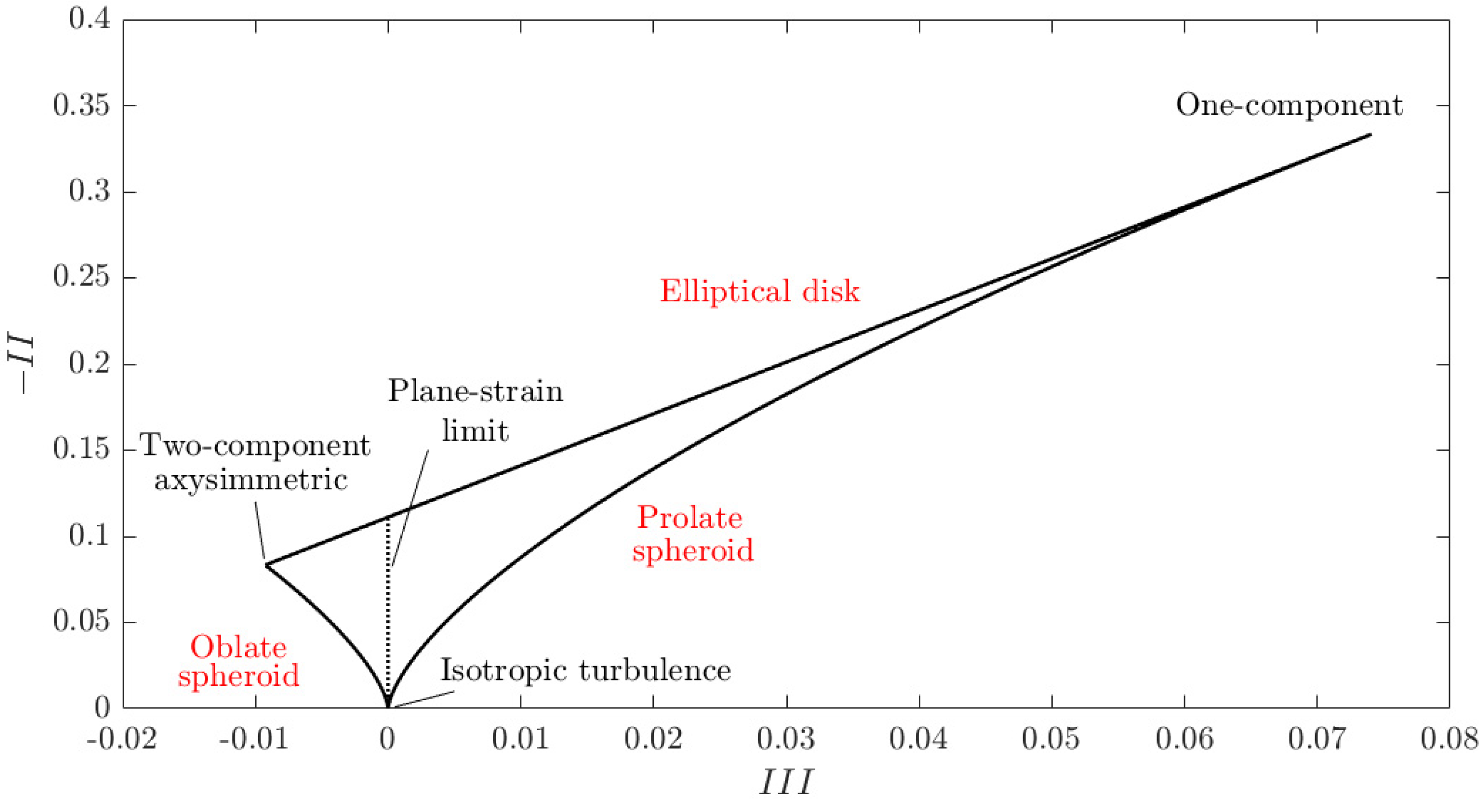
To characterize the type of turbulence, one of the most used methodologies is the definition of the Reynolds stress anisotropy tensor. In particular, the diagonalization of the tensor provides three eigenvalues (λ1, λ2, and λ3) and three eigenvectors (e1, e2, and e3) of the turbulence anisotropy [19]. The anisotropy invariant map (AIM) describes the domain of all potential turbulent flows considering the second and third invariants. In fact, it is a 2D domain with a triangular shape, whose boundaries are characteristic of turbulence state (1D, 2D, and 3D turbulence) and related processes (axisymmetric expansion, axisymmetric contraction, and two-component turbulence) [3].
Hence, the driving idea of the present study was the description of the turbulence anisotropy (with the AIMs) of flows through emergent rigid vegetation on rough beds. Indeed, exploring for the first time this crucial aspect in vegetated flows may advance the current understanding of the flow–vegetation–roughness interaction by describing the evolution of the stress ellipsoid formed by the Reynolds stresses. To this end, an experimental campaign was performed in a uniformly vegetated channel varying the bed sediment size (coarse sand, fine gravel, and coarse gravel), under the same hydraulic conditions. Additionally, in order to better comprehend the overall flow conditions, the time-averaged velocity, the Reynolds shear stresses, the viscous stresses, and the vorticity fields were analyzed and briefly discussed.
2. Experimental Program
2.1. Flume Set-Up and Bed Sediments
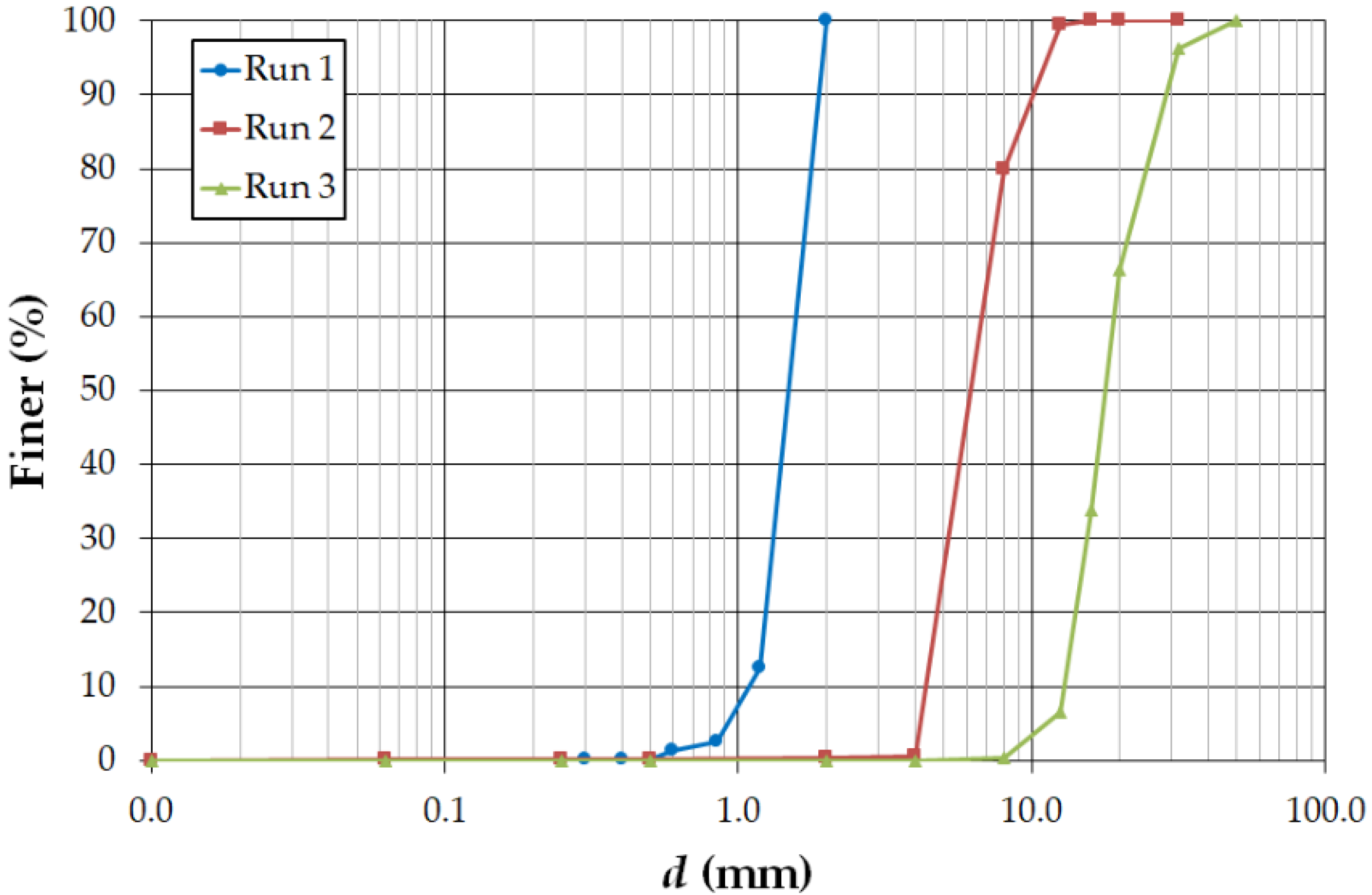
The experimental study was performed in a 9.6 m long, 0.485 m wide, and 0.5 m deep flow recirculating tilting flume at the Laboratorio “Grandi Modelli Idraulici” (GMI), Università della Calabria, Rende, Italy. Three experimental runs were performed under the same approach flow conditions and with the same vegetation arrangement, but with different bed sediments. In particular, the flume bed was covered with a 20 cm thick layer of uniform, very coarse sand (d50 = 1.53 mm), fine gravel (d50 = 6.49 mm), and coarse gravel (d50 = 17.98 mm) for Runs 1, 2, and 3, respectively. Figure 1 shows the grain-size distribution of the mixtures used to create the bed, which were obtained by analyzing three samples for each Run.
The flow rate Q was controlled by a submerged pump. It was measured using a calibrated sharp-crested V notch weir installed in a downstream tank, where the outflow was collected. To reduce the disturbance at the flume entrance and to dampen the related turbulence level, honeycombs with a diameter of 10 mm were used. The flume slope was set equal to 1.5‰ by maneuvering a hydraulic jack. Furthermore, the flow depth h was regulated with a downstream tailgate and measured with a point gauge.
The experimental runs were carried out by using a uniformly distributed vegetated channel bed, where the emergent vegetation was simulated with vertical, rigid, and circular wooden cylinders. A total number of 68 cylinders, each 2 cm in diameter, were inserted into a 1.96 m long, 0.485 m wide, and 0.015 m thick Plexiglas panel, which in turn was fixed to the channel bottom. The test section was located 6 m downstream of the flume inlet. The cylinders were arranged in an aligned pattern where the axis-to-axis distance between the stems was equal to 12 cm in both the streamwise and spanwise directions. Therefore, the total number of stems per unit area was 71.6 m−2. The frontal area per canopy volume was a = d/ΔS2 = 1.4 m−1, where d is the stem diameter and ΔS the axis-to-axis distance between the stems. The solid volume fraction occupied by the stems was ϕ = (π/4)ad = 0.02; thus, the vegetation can be considered as dense [21]. Further details of the experimental setup were recently reported by Penna et al. [18].
2.2. Experimental Procedure
Initially, the flume was filled in with sediments and was subsequently screeded flat to obtain a bed with a mean surface elevation having the same longitudinal slope of the channel. All the experimental runs initiated with a steady flow rate equal to 19.73 l s−1 and a water depth of 14 cm (measured 50 cm upstream to the vegetation array), designed to prevent sediments motions and to satisfy the fixed bed condition. Thus, the average flow velocity U was 0.30 m s−1 (=Q/(Bh), where B is the flume width) and the flow Froude number Fr was 0.26 (=U/(gh)0.5, where g is the gravitational acceleration). For each run, Table 1 shows the details of the experimental conditions for the approaching flow (measured 50 cm upstream to the test section), where u* is the shear velocity determined extending the linear trend of the Reynolds shear stress (RSS) distribution down to the maximum crest level (=, where u′ and w′ are the temporal velocity fluctuations in the streamwise and vertical directions, respectively, and the symbol indicates the time average), T is the water temperature (measured with an integrated thermometer with an accuracy of 0.1 °C) and ν is the water kinematic viscosity, determined as a function of the water temperature [22]. Furthermore, the Reynolds number of the sediments Re* (=u*ε/ν, where ε is the equivalent Nikuradse sand roughness height, equal to about 2d50) and the Reynolds number of the vegetation stems Red (=Ud/ν, where d is the stem diameter) were calculated.
The instantaneous three-dimensional flow velocity components were measured with a down-looking Vectrino probe (Acoustic Doppler Velocimeter, ADV) manufactured by Nortek, Vangkroken, Norway. The measurements were performed along the flume centerline at various relative streamwise distances x/Ls = 0, 0.17, 0.33, 0.50, 0.67, 0.83, 1.00, where x is the streamwise direction and Ls is the length of the study area equal to 12 cm. Note that x/Ls = 0 is the origin of the study area, located 6.78 m downstream of the channel entrance, and x/Ls = 0.50 corresponds to the vegetation stem axis. The 3D velocity components (u, v, w) refer to (x, y, z), where y and z are the spanwise and vertical direction, respectively.
The ADV probe was installed on a motorized 3-axis traverse system (HR Wallingford Ltd., Wallingford, Oxfordshire, UK) to easily move the probe within the study area during the experimental run. The Vectrino was operated with a transmitting length of 0.3 mm and a sampling volume constituted of a cylinder of 6 mm in diameter and 1 mm high. The sampling duration was equal to 180 s (the sampling frequency was fixed to 100 Hz), assuring statistically time-independent time-averaged velocities and turbulence quantities. It was not possible to perform velocity measurements within the flow zone 5 cm below the free surface, because the ADV beams converge at 5 cm below the probe. Thus, the vertical resolutions were 3 mm for mm and 5 mm above, where z is the vertical axis starting from the maximum crest elevation in the study area.
The ADV data were pre-processed for detecting potential spikes with the phase-space thresholding method. Spikes were replaced with a third-order polynomial through 12 points on both sides of the spike itself, as suggested by Goring and Nikora [23].
3. Results and Discussion
3.1. Time-Averaged Flow
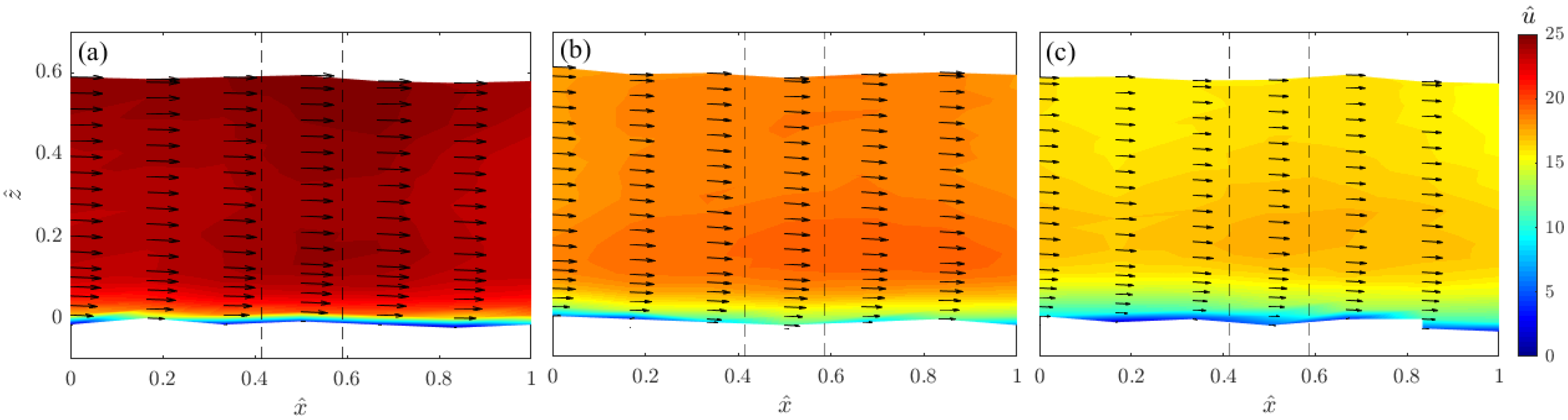
The dimensionless time-averaged velocity fields and 2D velocity vectors, having magnitude (where and are the time-averaged velocity components) and direction , on the vertical central plane are illustrated in Figure 2 for each Run. Here, the horizontal axis is represented as , and the vertical axis was made dimensionless dividing z by the local flow depth .
In Figure 2, a streamwise variation of the velocity field is detected in the three Runs. Specifically, in correspondence of the vegetation stem, increases with respect to the areas upstream to and downstream of the cylinder. This denotes the presence of: (1) a convergent flow between two stems and toward the flume centerline [24]; (2) a retarded flow owing to a divergent flow downstream of the stems. The changes of magnitude and direction of velocity vectors suggest the presence of a near-bed flow heterogeneity, which are more pronounced looking from Run 3 to Run 1. The streamwise and vertical variations of the velocity field is in agreement with Maji et al. [17], since significant velocity gradients were found in all the experimental runs. This is due to the different bed roughness that characterizes the three experimental runs. In essence, the flow velocity increases with the vertical distance, reaching the maximum values in correspondence of the vegetation stem and at the elevation , regardless of the bed roughness, implying that this region is mainly influenced by the presence of vegetation. Here, the production of turbulence by the canopy exceeds the production by the bed shear [21].
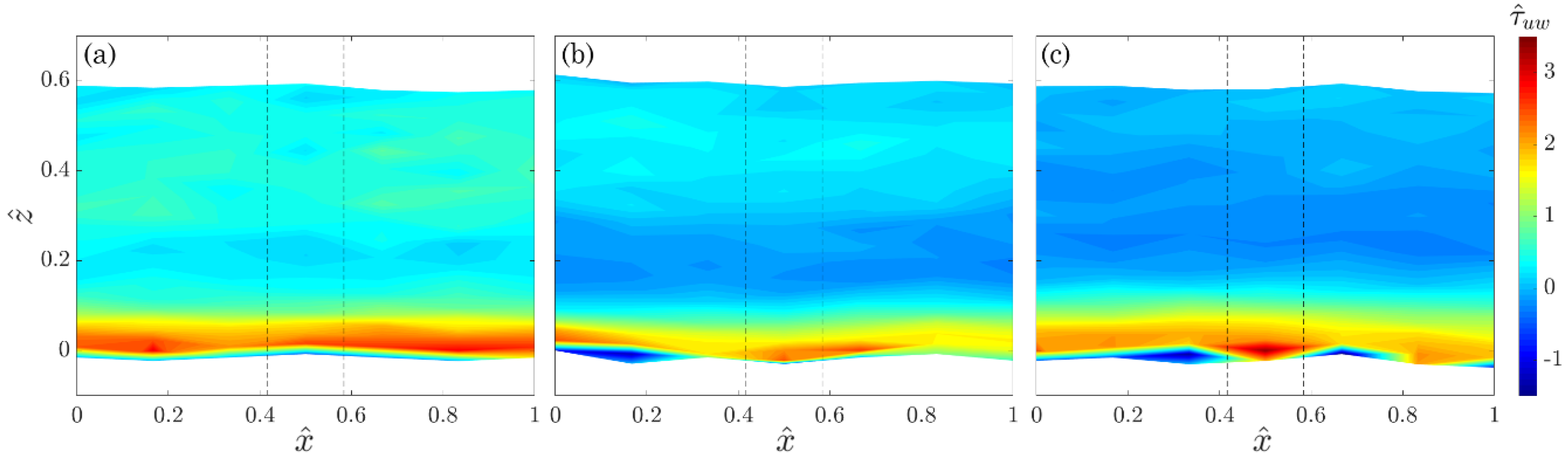
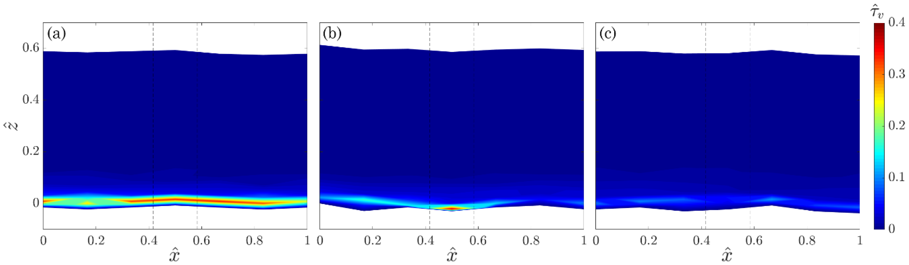
Figure 3 presents the contours of the dimensionless Reynolds shear stresses () on the vertical central plane for the three experimental Runs. They exhibit small magnitudes in the flow area dominated by the vegetation (for ) [6]. Moving toward the bed surface, the Reynolds shear stresses increase with a high gradient, owing to the bed roughness. As d50 increases, this zone becomes more extended. However, close to the bed at the crest level, the Reynolds shear stresses become negligible. The contours of reveal that they are not influenced by the position of vegetation stems, since their spatial distribution is quite uniform. Indeed, this agrees with the findings of Ricardo et al. [6], who demonstrated that the Reynolds stresses are not sensitive to local spatial gradients of the stem distribution, because they depend on the local number of stems per unit area. Analogous patterns can be noticed in Figure 4, where the dimensionless viscous stresses () on the vertical central plane for the three experimental Runs are presented. In fact, the streamwise distribution of is almost uniform in each Run. As the roughness decreases, the viscous shear stress increases at the crest level. Then, it diminishes as the vertical distance z increases. This agrees with the findings of Nepf [21], who stated that the viscous stress is negligible with respect to the vegetative drag over most of the depth, excluding a thin layer near the bed of a scale comparable to the stem diameter.
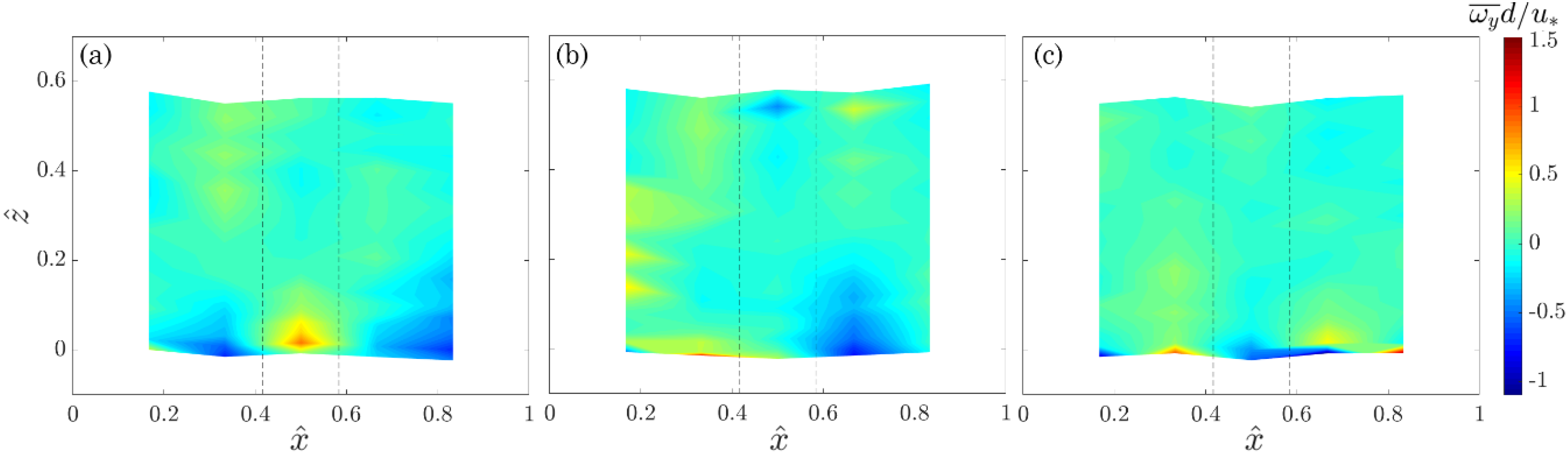
The effects of the bed roughness structures were investigated through the analysis of the dimensionless vorticity of the time-averaged flow on the vertical central plane (Figure 5). Here, is the vorticity of the time-averaged flow, given by . Positive values of the vorticity indicate clockwise fluid motion; on the contrary, negative values refer to counterclockwise direction. Specifically, the rotational direction provides information about flow acceleration and deceleration in the near-bed flow: counterclockwise rotation induces flow acceleration, with a downward transport of momentum in the downstream direction; clockwise rotation causes flow deceleration, with upward transport of momentum in the upstream direction [25,26]. It is evident that the vorticity changes its signs alternatively in the flow layer affected by the presence of both vegetation and bed roughness. This implies the heterogeneity of the time-averaged near-bed flow: fluid streaks move alternatively in both clockwise and counterclockwise directions [25]. Furthermore, it is possible to note that the changes of the vorticity rotational direction are more frequent in Run 1 than in the other two runs along the streamwise direction. As observed by Ricardo et al. [27], the cylinders induce a regular structure of vortex patterns independently from the space between cylinders also in the horizontal plane.
3.2. Anisotropy Invariant Maps
To investigate the anisotropic behavior of the flow through emergent rigid vegetation on rough beds, the AIM was examined along the flume centerline.
Originally introduced by Lumley and Newman [28], this map (also called the Lumley triangle) is a two-dimensional domain based on the invariant properties of the Reynolds stress anisotropy tensor bij, which can be defined as follows:
where is the Kronecker delta function ( and ) and, adopting the Einstein notation, is twice the TKE. The shape of the AIM is a triangle on a (III, −II) plane (Figure 6), where II is the second invariant of bij and represents the degree of anisotropy and III is the third invariant of bij and signifies the nature of anisotropy.
The two invariants can be expressed, respectively, as follows:
where and are the anisotropy eigenvalues.
The AIM is delimited by two curves and an upper line. The left curve is characterized by negative values of the third invariant and can be described as follows: III = −2(−II/3)3/2. This curve refers to the pancake-shaped turbulence, since two diagonal components of the Reynolds stress tensor are greater than the third one. The right curve is defined as III = 2(−II/3)3/2 and corresponds to the cigar-shaped turbulence, that is, one diagonal component of the Reynolds stress tensor is greater than the other two. Lastly, the function that expresses the upper line is III = −(9II + 1)/27; it describes a two-component turbulence. The bottom cusp of the AIM indicates, instead, the 3D isotropic turbulence.
Recently, Dey et al. [29] proposed an additional classification of the turbulence anisotropy, considering the shape of the ellipsoid formed by the Reynolds principal stresses σuu, σvv, and σww along the x-, y-, and z-axis, respectively. The Reynolds principal stresses are expressed respectively as , and , where is the mass density of water and v’ is the temporal fluctuation of the velocity in the spanwise direction.
Specifically, in the case of σuu = σvv = σww, that is an isotropic turbulence, the stress ellipsoid is a sphere. If σuu = σvv > σww (on the left curve of the AIM, which is termed as the axisymmetric contraction limit), the stress ellipsoid takes the shape of an oblate spheroid. The two-component axisymmetric limit lies on the left vertex of the AIM, where the conditions σuu = σvv and σww = 0 prevail. In this case, the shape of the stress ellipsoid is a circular disk. On the right curve (the axisymmetric expansion limit), one component of the Reynolds stresses is larger than the other two (σuu = σvv < σww), thus the stress ellipsoid takes the form of a prolate spheroid. At the top boundary, which indicates the two-component limit, the stress ellipsoid is an elliptical disk, since σuu > σvv and σww = 0. Finally, the one-component limit lies on the right vertex, where only one component of Reynolds stress sustains (that is, σuu > 0 and σvv = σww = 0 or σww > 0 and σuu = σvv = 0). This means that the stress ellipsoid assumes the shape of a straight line.
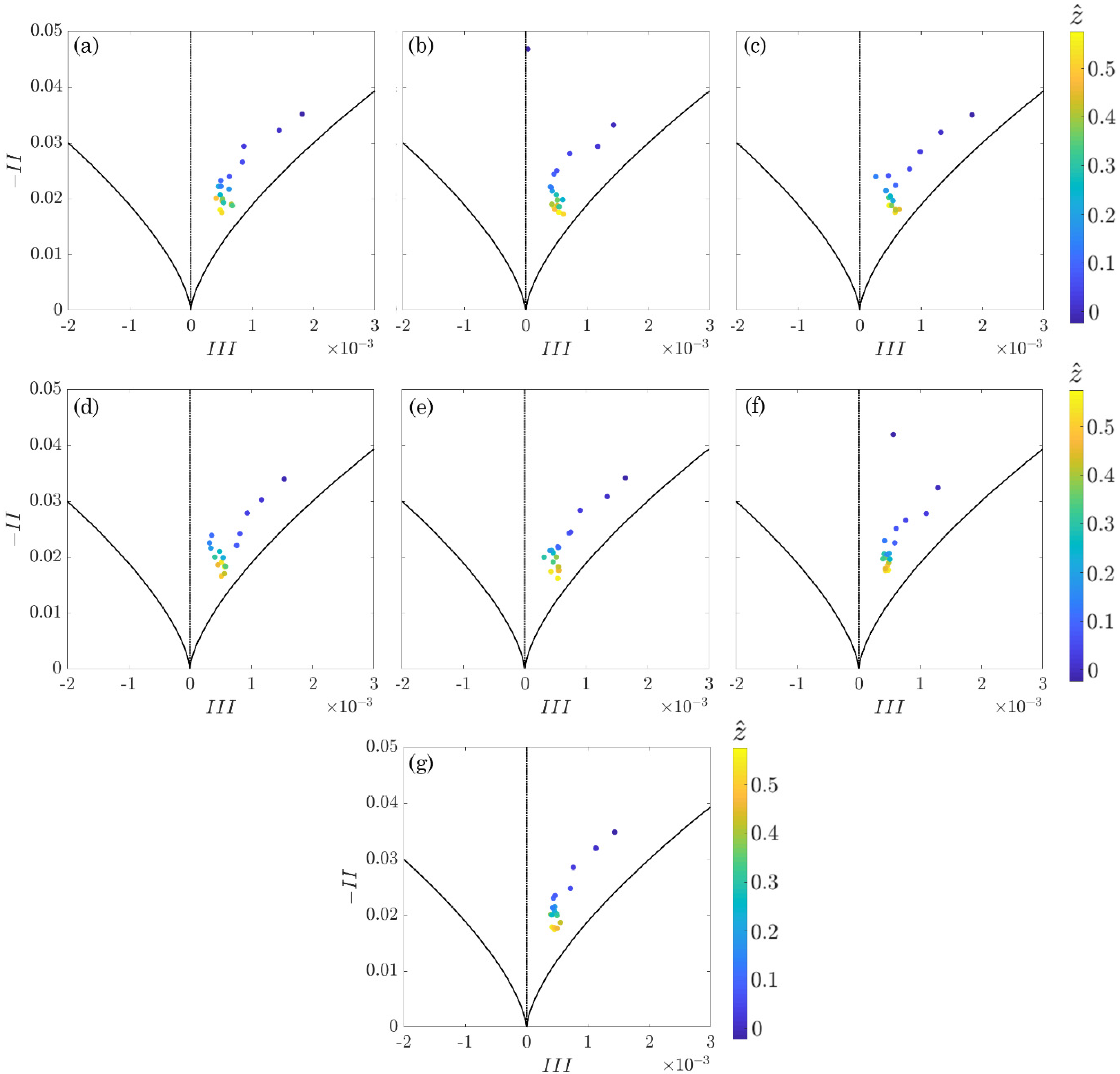
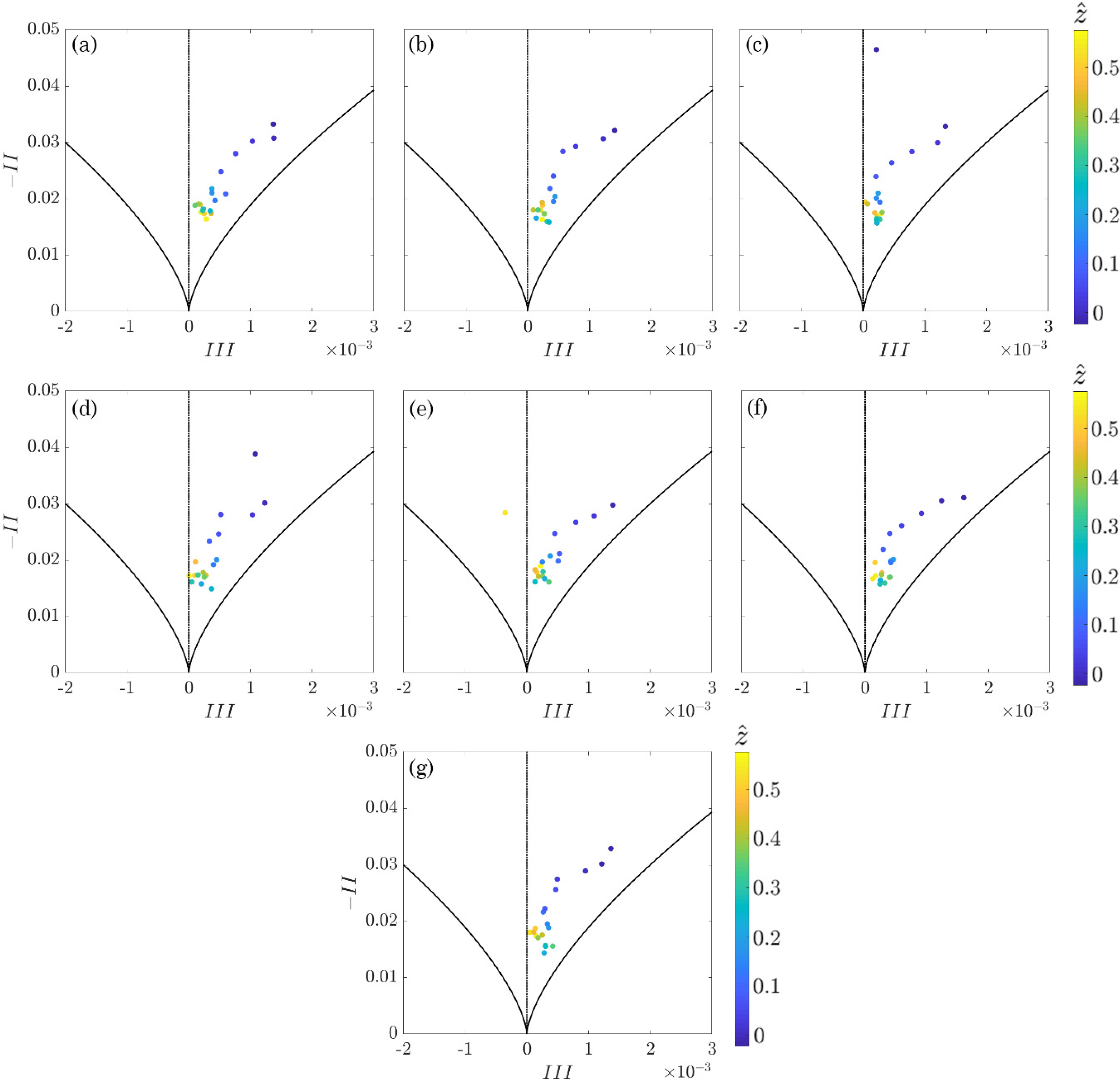
Figure 7 shows the data plots of −II versus III and the AIMs for Run 1, at the following streamwise relative distances: x/Ls = 0, 0.17, 0.33, 0.50, 0.67, 0.83, 1.00. Note that the plots were zoomed in the area of the AIM in which the data were concentrated. In the same way, Figure 8 and Figure 9 depict the AIMs for Runs 2 and 3, respectively. At a given streamwise distance, each subplot illustrates the evolution of the turbulence anisotropy along the dimensionless vertical distance . In all the Runs, moving from the crest level upwards, the data points of the Reynolds stress tensor describe a particular path, with some differences as the bed roughness changes.
Looking at Figure 7, near the bed, the turbulence anisotropy is prevalent as the data lie close to the right side of the Lumley triangle. This means that the velocity fluctuation in the vertical direction predominates owing to the bed roughness height, which enhances σww. Then, the data plots move toward the line of plane-strain limit, which is characterized by the condition III = 0. As the vertical distance increases, the turbulence anisotropy shows a feeble tendency again toward the axisymmetric expansion limit. The described path occurs at each streamwise distance, implying a similar behavior of the Reynolds stress tensor, regardless of the location with respect to the vegetation stem. Therefore, considering the classification based on the ellipsoid shape [29], it is evident that, near the bed, a prolate spheroid axisymmetric turbulence is predominant. Subsequently, as the vertical distance increases, an axisymmetric contraction develops, tending to the 3D isotropic turbulence in the region mainly affected by the vegetation.
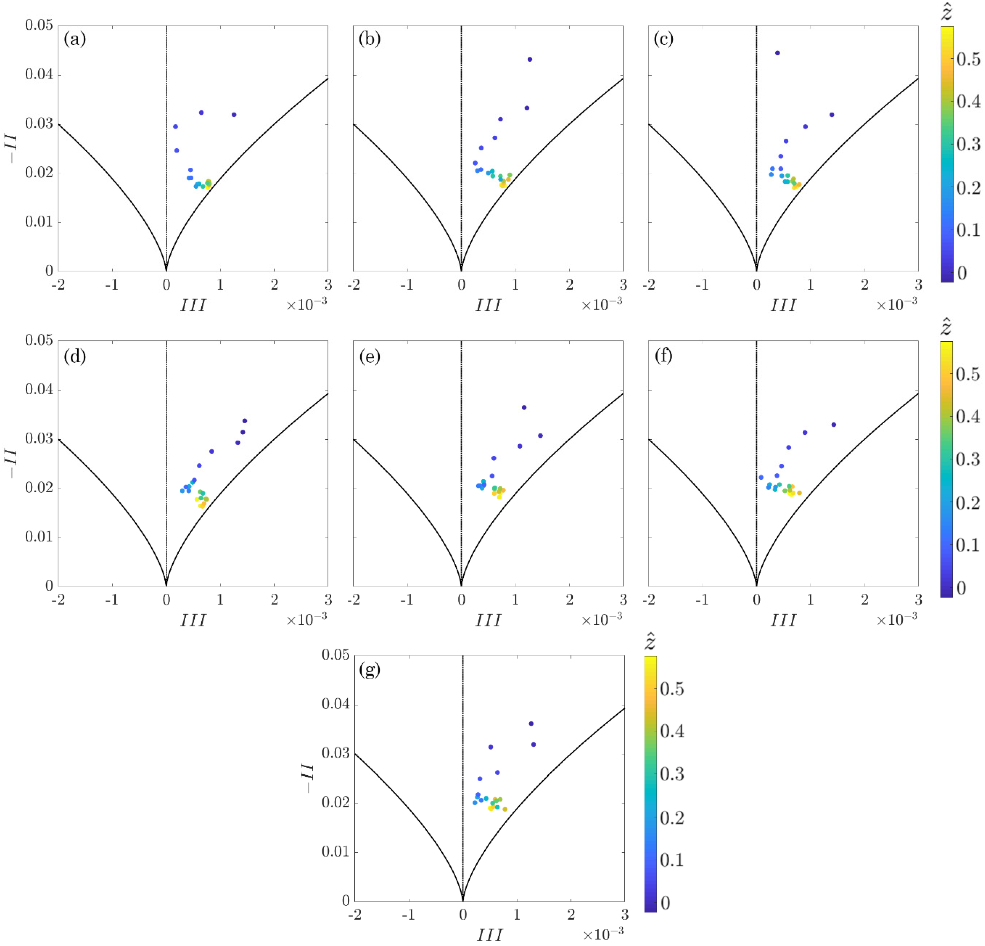
As regards Run 2, although near the crest level, the position of the data points in the AIMs does not vary from that of Run 1; moving toward the free surface, their path slightly changes. In fact, it is evident that the data plots tend to move toward the line of plane-strain limit, but they rapidly turn back to the right side of the Lumley triangle. This implies that one component of the Reynold stresses prevails on the others for almost the entire investigated flow depth. Thus, in Run 2, the ellipsoid is basically a prolate spheroid along . The same trend is visible at the different streamwise distances.
Akin to both Runs 1 and 2, the data plots of Run 3 start from the axisymmetric expansion limit (that corresponds to the right-curved side of the triangle). Increasing the vertical distance, they rapidly move toward the line of plane-strain limit. Then, the turbulence anisotropy tends to the isotropic state (the data move toward the bottom cusp of the AIM). This is due to the bed roughness influence on turbulence anisotropy, which vanishes moving toward the free surface. Thus, initially the ellipsoid shape is a prolate spheroid. As the vertical distance increases, an axisymmetric contraction develops, tending to the 3D isotropic state and, as a result, the stress ellipsoid becomes a sphere.
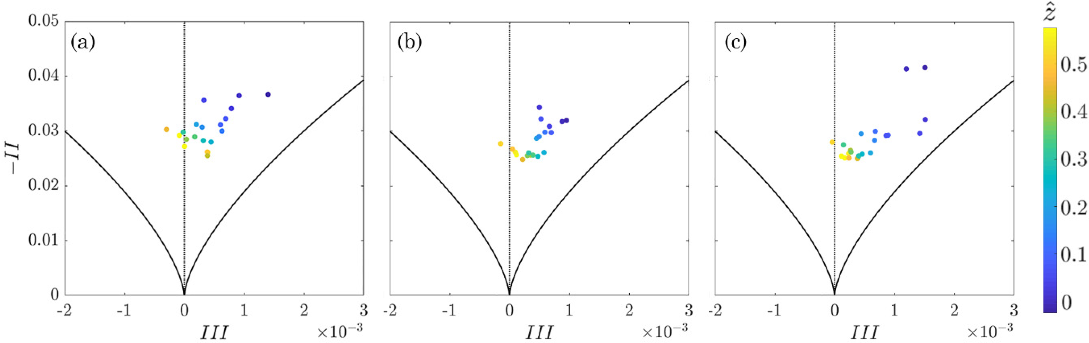
In order to highlight the effects induced by the presence of vegetation, Figure 10 shows the AIMs for the undisturbed flow conditions detected 50 cm upstream to the vegetation array in all the three Runs. It is revealed that, without the influence of vegetation, the turbulence anisotropy tends to the plane-strain limit in all the Runs, independently from the bed roughness, which, however, is the main cause of a prolate spheroid axisymmetric turbulence near the bed surface. This latter is more pronounced in Run 3, owing to a higher roughness height than in the other two Runs.
3.3. Anisotropic Invariant Function
Choi and Lumley [30] introduced a function, called the anisotropic invariant function F, with the aim of providing an insight into the turbulence anisotropy from the two-component limit to the isotropic limit [31]. The function can be calculated as follows:
The main peculiarity of the anisotropic invariant function is that it vanishes when the turbulence anisotropy prevails (F = 0), whereas it reaches unity (F = 1) when the turbulence reaches the three-dimensional isotropic state.
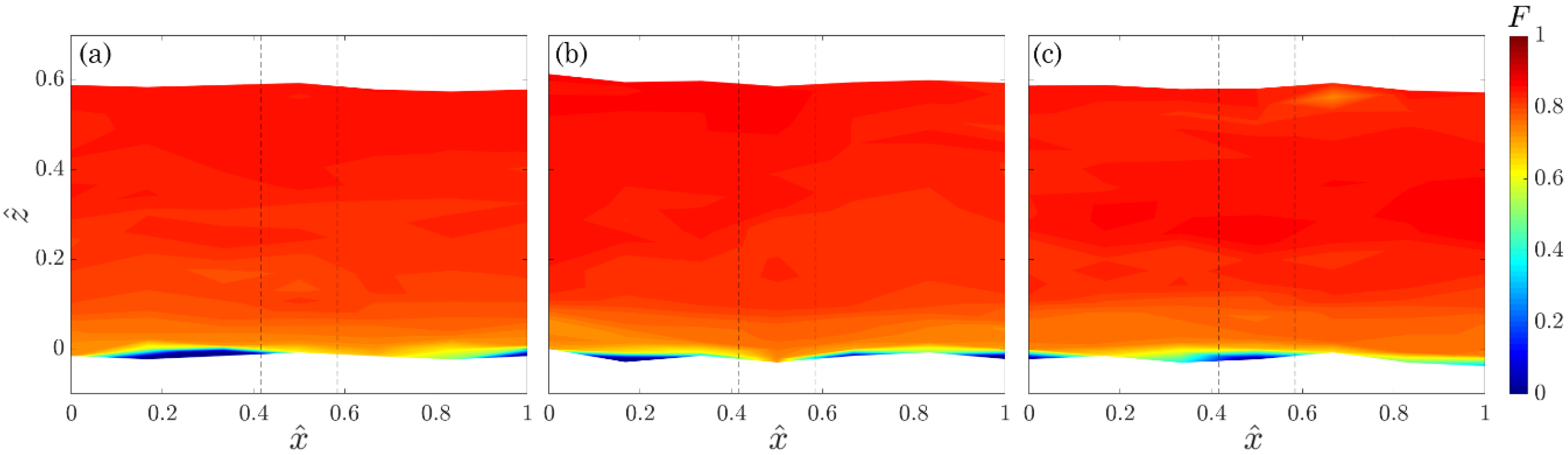
The contours of the anisotropic invariant function on the vertical central plane in the test section are shown in Figure 11 for all the Runs. The streamwise variation of the anisotropic invariant function is quite uniform, regardless of the location of the vegetation stem. However, it is possible to note that the topographical configuration of the bed surface has a strong impact on the turbulence characteristics of the flow. In fact, on the uphill stretches F is almost null, indicating a strong two-dimensional turbulence, since one velocity component is limited by the bed. Then, the anisotropic invariant function becomes greater than 0 on the downhill stretches, where the turbulence can develop in the three directions.
Moving toward the free surface, the anisotropic invariant function gradually increases, reaching approximately F = 0.9. This confirms that the bed roughness influence on turbulence anisotropy vanishes moving toward the free surface.
3.4. New Research Prospects
The experimental results obtained in this study represent a new dataset that may be used for the calibration of advanced numerical models, which are usually based on isotropic turbulence hypothesis. In fact, as it was demonstrated, vegetation and bed roughness can hinder flow by acting as an obstruction, generating turbulence, and affecting the entire flow velocity distribution [32], modifying the turbulence behavior from isotropic to anisotropic moving toward the bed surface.
The modelling of such vegetated flows on rough beds clearly gets complicated if natural and complex channel cross-sections with different shapes are considered. Recent researches showed that different rectangular and trapezoidal shapes as well as the corner angles can exert a strong impact on the flow velocity distribution and its induced secondary flow [33,34,35]; hence, they may affect the sediment transport process [36]. Therefore, new analytical models of sidewall turbulence effect on streamwise velocity profile have been recently proposed (e.g., [35,37]) for uneven narrow and wide channels. These analytical models could be improved by considering extra turbulence zones represented by both vegetation and rough beds.
However, flow structures become even more complex when vegetation appears in channels with bedforms [38]. How the existence of vegetation changes flow pattern over gravel bedforms still remains poorly understood and could be considered as another potential development of the present research work.
4. Conclusions
The aim of the present work was the study of the turbulence anisotropy in the free stream region of turbulent flows through rigid emergent vegetation on rough beds using AIMs. Three experimental runs were performed in a uniformly distributed vegetated channel with three different bed sediments. The principal findings are summarized below.
- Two different zones were characterized along the flume centerline: a convergent flow zone between two stems and toward the flume centerline; a retarded flow zone owing to a divergent flow downstream of the stems. Owing to the bed roughness, a near-bed flow heterogeneity was found, activating the fluid streaks to have motions alternatively in both clockwise and counterclockwise directions. Here, the Reynolds shear stresses increase with a high gradient, but at the crest level they become negligible and the viscous stresses reach their maximum values. However, the quite uniform streamwise distribution of both and reveal that they were not influenced by the position of vegetation stems.
- The analysis of the AIMs revealed that the combined effect of vegetation and bed roughness causes the evolution of the turbulence from the quasi-three-dimensional isotropy (the stress ellipsoid is like a sphere) to a prolate spheroid axisymmetric turbulence. This kind of turbulence anisotropy is kept also near the bed surface. This particular pattern is also confirmed by the contours of the anisotropic invariant function.
- The topographical configuration of the bed surface has a strong impact on the turbulent characteristics of the flow. In fact, on the uphill stretches, the anisotropic invariant function indicates a strong two-dimensional turbulence, since one velocity component is limited by the bed surface. Instead, on the downhill stretches, the anisotropic invariant function reveals that the turbulence can develop in the three directions.
Author Contributions
Conceptualization, N.P., F.C., A.D., R.G.; methodology, N.P., F.C., A.D., R.G.; formal analysis, N.P., F.C.; data curation, F.C.; writing—original draft preparation, N.P.; writing—review and editing, N.P., F.C., A.D., R.G.; supervision, R.G.; funding acquisition, R.G. All authors have read and agreed to the published version of the manuscript.
Funding
This research was funded by the “PreFluSed—Prevenzione del rischio di alluvioni in un bacino Fluviale calabrese in presenza di trasporto di Sedimenti” Project (Ministero dell’Ambiente e della Tutela del Territorio e del Mare, Direzione Generale per la Salvaguardia del Territorio e delle Acque, Italy).
Acknowledgments
The authors would like to thank Davide Garigliano for his valuable work during the performance of the experimental runs and the anonymous referees for their suggestions and comments.
Conflicts of Interest
The authors declare no conflict of interest.
References
- White, B.L.; Nepf, H.M. A vortex-based model of velocity and shear stress in a partially vegetated shallow channel. Water Resour. Res. 2008, 44, 1–15. [Google Scholar] [CrossRef]
- Ben Meftah, M.; De Serio, F.; Mossa, M. Hydrodynamic behavior in the outer shear layer of partly obstructed open channels. Phys. Fluids 2014, 26, 065102. [Google Scholar] [CrossRef]
- Caroppi, G.; Gualtieri, P.; Fontana, N.; Giugni, M. Vegetated channel flows: Turbulence anisotropy at flow–rigid canopy interface. Geosciences 2018, 8, 259. [Google Scholar] [CrossRef] [Green Version]
- Rowiński, P.M.; Västilä, K.; Aberle, J.; Järvelä, J.; Kalinowska, M.B. How vegetation can aid in coping with river management challenges: A brief review. Ecohydrol. Hydrobiol. 2018, 18, 345–354. [Google Scholar] [CrossRef] [Green Version]
- Caroppi, G.; Västilä, K.; Järvelä, J.; Rowiński, P.M.; Giugni, M. Turbulence at water-vegetation interface in open channel flow: Experiments with natural-like plants. Adv. Water Resour. 2019, 127, 180–191. [Google Scholar] [CrossRef]
- Ricardo, A.M.; Franca, M.J.; Ferreira, R.M. Turbulent flows within random arrays of rigid and emergent cylinders with varying distribution. J. Hydraul. Eng. 2016, 142, 04016022. [Google Scholar] [CrossRef]
- Schoelynck, J.; De Groote, T.; Bal, K.; Vandenbruwaene, W.; Meire, P.; Temmerman, S. Self-organised patchiness and scale dependent bio-geomorphic feedbacks in aquatic river vegetation. Ecography 2012, 35, 760–768. [Google Scholar] [CrossRef]
- Bearman, P.W.; Zdravkovich, M.M. Flow around a circular cylinder near a plane boundary. J. Fluid Mech. 1978, 89, 33–47. [Google Scholar] [CrossRef]
- Nezu, I.; Sanjou, M. Turburence structure and coherent motion in vegetated canopy open-channel flows. J. Hydro-Environ. Res. 2008, 2, 62–90. [Google Scholar] [CrossRef]
- Yang, W.; Choi, S.U. A two-layer approach for depth-limited open-channel flows with submerged vegetation. J. Hydraul. Res. 2010, 48, 466–475. [Google Scholar] [CrossRef]
- Shimizu, Y.; Tsujimoto, T. Numerical analysis of turbulent open-channel flow over a vegetation layer using a k-ε turbulence model. J. Hydrosci. Hydraul. Eng. 1994, 11, 57–67. [Google Scholar]
- Nepf, H. Drag, turbulence, and diffusion in flow through emergent vegetation. Water Resour. Res. 1999, 35, 479–489. [Google Scholar] [CrossRef]
- Righetti, M.; Armanini, A. Flow resistance in open channel flows with sparsely distributed bushes. J. Hydrol. 2002, 269, 55–64. [Google Scholar] [CrossRef]
- Choi, S.U.; Kang, H. Numerical investigations of mean flow and turbulence structures of partly-vegetated open-channel flows using the Reynolds stress model. J. Hydraul. Res. 2006, 44, 203–217. [Google Scholar] [CrossRef]
- Poggi, D.; Krug, C.; Katul, G.G. Hydraulic resistance of submerged rigid vegetation derived from first-order closure models. Water Resour. Res. 2009, 45, W10442. [Google Scholar] [CrossRef]
- Gualtieri, P.; De Felice, S.; Pasquino, V.; Doria, G. Use of conventional flow resistance equations and a model for the Nikuradse roughness in vegetated flows at high submergence. J. Hydrol. Hydromech. 2018, 66, 107–120. [Google Scholar] [CrossRef] [Green Version]
- Maji, S.; Hanmaiahgari, P.R.; Balachandar, R.; Pu, J.H.; Ricardo, A.M.; Ferreira, R.M. A Review on Hydrodynamics of Free Surface Flows in Emergent Vegetated Channels. Water 2020, 12, 1218. [Google Scholar] [CrossRef]
- Penna, N.; Coscarella, F.; D’Ippolito, A.; Gaudio, R. Bed roughness effects on the turbulence characteristics of flows through emergent rigid vegetation. Water 2020, 12, 2401. [Google Scholar] [CrossRef]
- Emory, M.; Iaccarino, G. Visualizing turbulence anisotropy in the spatial domain with componentality contours. Cent. Turbul. Res. Annu. Res. Briefs 2014, 123–138. [Google Scholar]
- Sarkar, S.; Ali, S.Z.; Dey, S. Turbulence in Wall-Wake Flow Downstream of an Isolated Dunal Bedform. Water 2019, 11, 1975. [Google Scholar] [CrossRef] [Green Version]
- Nepf, H.M. Flow and transport in regions with aquatic vegetation. Annu. Rev. Fluid Mech. 2012, 44, 123–142. [Google Scholar] [CrossRef] [Green Version]
- Julien, P.Y. Erosion and Sedimentation; Cambridge University Press: Cambridge, UK, 1998. [Google Scholar]
- Goring, D.G.; Nikora, V.I. Despiking acoustic Doppler velocimeter data. J. Hydraul. Eng. 2002, 128, 117–126. [Google Scholar] [CrossRef] [Green Version]
- De Serio, F.; Ben Meftah, M.; Mossa, M.; Termini, D. Experimental investigation on dispersion mechanisms in rigid and flexible vegetated beds. Adv. Water Resour. 2018, 120, 98–113. [Google Scholar] [CrossRef]
- Padhi, E.; Penna, N.; Dey, S.; Gaudio, R. Near-bed turbulence structures in water-worked and screeded gravel-bed flows. Phys. Fluids 2019, 31, 045107. [Google Scholar] [CrossRef]
- Penna, N.; Coscarella, F.; Gaudio, R. Turbulent Flow Field around Horizontal Cylinders with Scour Hole. Water 2020, 12, 143. [Google Scholar] [CrossRef] [Green Version]
- Ricardo, A.M.; Koll, K.; Franca, M.J.; Schleiss, A.J.; Ferreira, R.M.L. The terms of turbulent kinetic energy budget within random arrays of emergent cylinders. Water Resour. Res. 2014, 50, 4131–4148. [Google Scholar] [CrossRef]
- Lumley, J.L.; Newman, G.R. The return to isotropy of homogeneous turbulence. J. Fluid Mech. 1977, 82, 161–178. [Google Scholar] [CrossRef] [Green Version]
- Dey, S.; Ravi Kishore, G.; Castro-Orgaz, O.; Ali, S.Z. Turbulent length scales and anisotropy in submerged turbulent plane offset jets. J. Hydraul. Eng. 2019, 145, 04018085. [Google Scholar] [CrossRef]
- Choi, K.S.; Lumley, J.L. The return to isotropy of homogeneous turbulence. J. Fluid Mech. 2001, 436, 59–84. [Google Scholar] [CrossRef]
- Penna, N.; Padhi, E.; Dey, S.; Gaudio, R. Structure functions and invariants of the anisotropic Reynolds stress tensor in turbulent flows on water-worked gravel beds. Phys. Fluids 2020, 32, 055106. [Google Scholar] [CrossRef]
- Pu, J.H.; Hussain, A.; Guo, Y.K.; Vardakastanis, N.; Hanmaiahgari, P.R.; Lam, D. Submerged flexible vegetation impact on open channel flow velocity distribution: An analytical modelling study on drag and friction. Water Sci. Eng. 2019, 12, 121–128. [Google Scholar] [CrossRef]
- Lucas, J.; Lutz, N.; Lais, A.; Hager, W.H.; Boes, R.M. Side-channel flow: Physical model studies. J. Hydraul. Eng. 2017, 05015003, 1–11. [Google Scholar] [CrossRef]
- Vidal, A.; Nagib, H.M.; Schlatter, P.; Vinuesa, R. Secondary flow in spanwise periodic in-phase sinusoidal channels. J. Fluid Mech. 2018, 851, 288–316. [Google Scholar] [CrossRef]
- Pu, J.H.; Pandey, M.; Hanmaiahgari, P.R. Analytical modelling of sidewall turbulence effect on streamwise velocity profile using 2D approach: A comparison of rectangular and trapezoidal open channel flows. J. Hydro-Environ. Res. 2020. [Google Scholar] [CrossRef]
- Pu, J.H.; Lim, S.Y. Efficient numerical computation and experimental study of temporally long equilibrium scour development around abutment. Environ. Fluid Mech. 2014, 14, 69–86. [Google Scholar] [CrossRef] [Green Version]
- Pu, J.H. Turbulent rectangular compound open channel flow study using multi-zonal approach. Environ. Fluid Mech. 2019, 19, 785–800. [Google Scholar] [CrossRef] [Green Version]
- Afzalimehr, H.; Maddahi, M.R.; Sui, J.; Rahimpour, M. Impacts of vegetation over bedforms on flow characteristics in gravel-bed rivers. J. Hydrodyn. 2019, 31, 986–998. [Google Scholar] [CrossRef]
Figure 1.
Grain-size distribution curve of the bed sediments for each experimental run.

Figure 2.
Contours of dimensionless time-averaged velocity and 2D velocity vectors measured on the vertical central plane for (a) Run 1, (b) Run 2, and (c) Run 3. The black broken lines indicate the edge of the vegetation stem.
Figure 2.
Contours of dimensionless time-averaged velocity and 2D velocity vectors measured on the vertical central plane for (a) Run 1, (b) Run 2, and (c) Run 3. The black broken lines indicate the edge of the vegetation stem.

Figure 3.
Contours of dimensionless Reynolds shear stresses measured on the vertical central plane for (a) Run 1, (b) Run 2, and (c) Run 3. The black broken lines indicate the edge of the vegetation stem.
Figure 3.
Contours of dimensionless Reynolds shear stresses measured on the vertical central plane for (a) Run 1, (b) Run 2, and (c) Run 3. The black broken lines indicate the edge of the vegetation stem.

Figure 4.
Contours of dimensionless viscous shear stresses measured on the vertical central plane for (a) Run 1, (b) Run 2, and (c) Run 3. The black broken lines indicate the edge of the vegetation stem.
Figure 4.
Contours of dimensionless viscous shear stresses measured on the vertical central plane for (a) Run 1, (b) Run 2, and (c) Run 3. The black broken lines indicate the edge of the vegetation stem.

Figure 5.
Contours of dimensionless vorticity of the time-averaged flow in the vertical central plane for (a) Run 1, (b) Run 2, and (c) Run 3. The black broken lines indicate the edge of the vegetation stem.
Figure 5.
Contours of dimensionless vorticity of the time-averaged flow in the vertical central plane for (a) Run 1, (b) Run 2, and (c) Run 3. The black broken lines indicate the edge of the vegetation stem.

Figure 6.
Conceptual diagram of the anisotropy invariant map.

Figure 7.
AIMs of Run 1 at (a) x/Ls = 0, (b) x/Ls = 0.17, (c) x/Ls = 0.33, (d) x/Ls = 0.50 (at the vegetation stem axis), (e) x/Ls = 0.67, (f) x/Ls = 0.83, (g) x/Ls = 1.00.
Figure 7.
AIMs of Run 1 at (a) x/Ls = 0, (b) x/Ls = 0.17, (c) x/Ls = 0.33, (d) x/Ls = 0.50 (at the vegetation stem axis), (e) x/Ls = 0.67, (f) x/Ls = 0.83, (g) x/Ls = 1.00.

Figure 8.
AIMs of Run 2 at (a) x/Ls = 0, (b) x/Ls = 0.17, (c) x/Ls = 0.33, (d) x/Ls = 0.50 (at the vegetation stem axis), (e) x/Ls = 0.67, (f) x/Ls = 0.83, (g) x/Ls = 1.00.
Figure 8.
AIMs of Run 2 at (a) x/Ls = 0, (b) x/Ls = 0.17, (c) x/Ls = 0.33, (d) x/Ls = 0.50 (at the vegetation stem axis), (e) x/Ls = 0.67, (f) x/Ls = 0.83, (g) x/Ls = 1.00.

Figure 9.
AIMs of Run 3 at (a) x/Ls = 0, (b) x/Ls = 0.17, (c) x/Ls = 0.33, (d) x/Ls = 0.50 (at the vegetation stem axis), (e) x/Ls = 0.67, (f) x/Ls = 0.83, (g) x/Ls = 1.00.
Figure 9.
AIMs of Run 3 at (a) x/Ls = 0, (b) x/Ls = 0.17, (c) x/Ls = 0.33, (d) x/Ls = 0.50 (at the vegetation stem axis), (e) x/Ls = 0.67, (f) x/Ls = 0.83, (g) x/Ls = 1.00.

Figure 10.
AIMs of the undisturbed flow condition for (a) Run 1, (b) Run 2, and (c) Run 3.

Figure 11.
Contours of the anisotropic invariant function F in the test section for (a) Run 1, (b) Run 2, and (c) Run 3. The black broken lines indicate the edge of the vegetation stem.
Figure 11.
Contours of the anisotropic invariant function F in the test section for (a) Run 1, (b) Run 2, and (c) Run 3. The black broken lines indicate the edge of the vegetation stem.


Table 1.
Details of the experimental conditions.
| Run | d50 (mm) | u* (m s−1) | T (°C) | ν (m2 s) | Re* | Red |
|---|---|---|---|---|---|---|
| 1 | 1.53 | 0.017 | 21.70 | 9.63 × 10⁻⁷ | 54 | 6231 |
| 2 | 6.49 | 0.022 | 21.44 | 9.69 × 10⁻⁷ | 295 | 6192 |
| 3 | 17.98 | 0.028 | 20.80 | 9.83 × 10⁻⁷ | 1024 | 6104 |
© 2020 by the authors. Licensee MDPI, Basel, Switzerland. This article is an open access article distributed under the terms and conditions of the Creative Commons Attribution (CC BY) license (http://creativecommons.org/licenses/by/4.0/).
Share and Cite
MDPI and ACS Style
Penna, N.; Coscarella, F.; D’Ippolito, A.; Gaudio, R. Anisotropy in the Free Stream Region of Turbulent Flows through Emergent Rigid Vegetation on Rough Beds. Water 2020, 12, 2464. https://doi.org/10.3390/w12092464
AMA Style
Penna N, Coscarella F, D’Ippolito A, Gaudio R. Anisotropy in the Free Stream Region of Turbulent Flows through Emergent Rigid Vegetation on Rough Beds. Water. 2020; 12(9):2464. https://doi.org/10.3390/w12092464
Chicago/Turabian StylePenna, Nadia, Francesco Coscarella, Antonino D’Ippolito, and Roberto Gaudio. 2020. "Anisotropy in the Free Stream Region of Turbulent Flows through Emergent Rigid Vegetation on Rough Beds" Water 12, no. 9: 2464. https://doi.org/10.3390/w12092464
Note that from the first issue of 2016, this journal uses article numbers instead of page numbers. See further details here.