Article

Lag Time as an Indicator of the Link between Agricultural Pressure and Drinking Water Quality State

1
Department of Quaternary and Groundwater Mapping, Geological Survey of Denmark and Greenland (GEUS), C.F. Møllers Allé 8, Building 1110, 8000 Aarhus C, Denmark
2
BRGM, 3, avenue C. Guillemin, BP 360009, 45060 Orléans CEDEX 2, France
3
Department of Agroecology, Aarhus University, Blichers Alle 20, 8830 Tjele, Denmark
4
Department of Bioscience, Aarhus University, Vejlsøvej 25, 8600 Silkeborg, Denmark
*
Author to whom correspondence should be addressed.
Water 2020, 12(9), 2385; https://doi.org/10.3390/w12092385
Submission received: 14 July 2020 / Revised: 14 August 2020 / Accepted: 19 August 2020 / Published: 25 August 2020
(This article belongs to the Special Issue Land Use and Water Quality)

Abstract

:
Diffuse nitrogen (N) pollution from agriculture in groundwater and surface water is a major challenge in terms of meeting drinking water targets in many parts of Europe. A bottom-up approach involving local stakeholders may be more effective than national- or European-level approaches for addressing local drinking water issues. Common understanding of the causal relationship between agricultural pressure and water quality state, e.g., nitrate pollution among the stakeholders, is necessary to define realistic goals of drinking water protection plans and to motivate the stakeholders; however, it is often challenging to obtain. Therefore, to link agricultural pressure and water quality state, we analyzed lag times between soil surface N surplus and groundwater chemistry using a cross correlation analysis method of three case study sites with groundwater-based drinking water abstraction: Tunø and Aalborg-Drastrup in Denmark and La Voulzie in France. At these sites, various mitigation measures have been implemented since the 1980s at local to national scales, resulting in a decrease of soil surface N surplus, with long-term monitoring data also being available to reveal the water quality responses. The lag times continuously increased with an increasing distance from the N source in Tunø (from 0 to 20 years between 1.2 and 24 m below the land surface; mbls) and La Voulzie (from 8 to 24 years along downstream), while in Aalborg-Drastrup, the lag times showed a greater variability with depth—for instance, 23-year lag time at 9–17 mbls and 4-year lag time at 21–23 mbls. These spatial patterns were interpreted, finding that in Tunø and La Voulzie, matrix flow is the dominant pathway of nitrate, whereas in Aalborg-Drastrup, both matrix and fracture flows are important pathways. The lag times estimated in this study were comparable to groundwater ages measured by chlorofluorocarbons (CFCs); however, they may provide different information to the stakeholders. The lag time may indicate a wait time for detecting the effects of an implemented protection plan while groundwater age, which is the mean residence time of a water body that is a mixture of significantly different ages, may be useful for planning the time scale of water protection programs. We conclude that the lag time may be a useful indicator to reveal the hydrogeological links between the agricultural pressure and water quality state, which is fundamental for a successful implementation of drinking water protection plans.

1. Introduction

The leaching of nitrate from intensive agricultural areas is one of the greatest threats to clean drinking water resources in Europe and the rest of the world. The groundwater and drinking water standard of nitrate is set to a maximum of 50 mg NO3/L in the European Union (EU), following the recommendations of the World Health Organization (WHO) [1]. This level is set to protect infants from the acute condition called blue baby syndrome (methemoglobinemia) [2,3]. However, recent studies have reported that long-term exposure to drinking water containing nitrate below the current standard is suspected to have chronic adverse effects [3,4,5,6]. For instance, studies have consistently reported that risks of colorectal cancer, thyroid disease, and central nervous system birth defects are strongly associated with ingestion of drinking water nitrate [3]. The EU has issued a series of directives, guidelines, and policies over the last decades to set the requirements of the drinking water standards (i.e., Drinking Water Directive) and to protect the drinking water resources (e.g., Water Framework Directive, Groundwater Directive, Nitrate Directive, and Directive on the Sustainable Use of Pesticides). Each country in the EU has implemented these legislations in their national laws differently, due to adjustment to local politico-socio-economic-agri-hydrogeological conditions [7,8]. The Drinking Water Directive primarily focuses on large water supplies. Small water supplies in rural areas have been given less attention, resulting in worse cases of drinking water quality [9,10].
The Organization for Economic Co-operation and Development (OECD) has proposed a bottom-up approach that integrates multiple local and regional stakeholders, such as farmers, citizens, drinking water suppliers, policy-makers, and scientists, as an effective approach for addressing local issues in relation to drinking water security, rather than the most common top-down approach at the national and EU level [11]. Research has also shown that the success of water protection plans depends on the social, technical, financial, and political capacity of the stakeholders and institutional arrangements, such as policies and regulations [12,13,14,15]. In addition, non-regulatory tools, such as training, information campaigns, education, or voluntary programs, have been shown to be effective in increasing the engagement of stakeholders and consequently lead to the successful implementation of water protection programs [12].
Common understandings of the cause and effect relations between the agricultural pressure and drinking water state may be a fundamental step in finding common and achievable goals among stakeholders and in planning drinking water protection programs [8,16,17]. However, the cause–effect relations are often difficult to identify. A long lag time between the use of fertilizer and its effects on water quality is often considered to be one of the reasons for unclear correlations between the agricultural pressure and water quality state [8,18,19]. When authorities and farmers implement mitigation measures (e.g., catch crops, set-aside, and buffer zones) as part of water protection planning, they may have to wait multiple decades to observe the effects on the water quality in some geological settings. Consequently, it may be inevitable that farmers become less engaged in water protection programs, unless they are well-informed in advance. In addition, information that is key to evaluating the cause–effect relations is monitored and managed by different institutions and government bodies [8]. Therefore, it is often difficult to gather coherent information to understand the complexity of the system.
The hydrogeological system that links the agricultural and drinking water systems may be the first-order control on regulating the relationships between these two systems; however, its importance has often been neglected in communication among stakeholders and the development of water protection plans. For example, the Driving force–Pressure–State–Impact–Response (DPSIR) framework is one of the most widely used conceptual frameworks in integrated water resource management to explain the causal relationships between society and the environment [20,21,22,23,24,25]. The DPSIR describes the feedback among social and economic developments, including the driving forces (D); pressures (P) on the environment; state (S) of environmental changes; impacts (I) on ecosystems, human health, and society; and a societal response (R) [26,27]. Under this framework, however, there is no component to explain the relationships between pressure and state, which may vary from site to site. The DPSIR framework has previously been criticized for not addressing the dynamics of the system, and others have argued that there should be a focus on the links between the nodes of the DPSIR [22,23,24,25].
In this study, therefore, we proposed a new component, named “Link”, for the DPSIR framework in order to better explain the interactions between pressure and state, called DPLSIR (Figure 1). Furthermore, we suggested the lag time between agricultural pressure (i.e., nitrate inputs from the agricultural system) and water state (i.e., nitrate concentrations in the hydrogeological system) as a key link indicator. The contaminant of interest is nitrate. The objectives of this study are to evaluate a cross-correlation function analysis as a simple methodology for estimating lag times using data from three case study site in Europe (two in Denmark and one in France) and then to investigate controls of the temporal scale and spatial heterogeneity of lag times to better characterize the hydrogeological link between agricultural pressure and water quality state.

2. Conceptual Framework

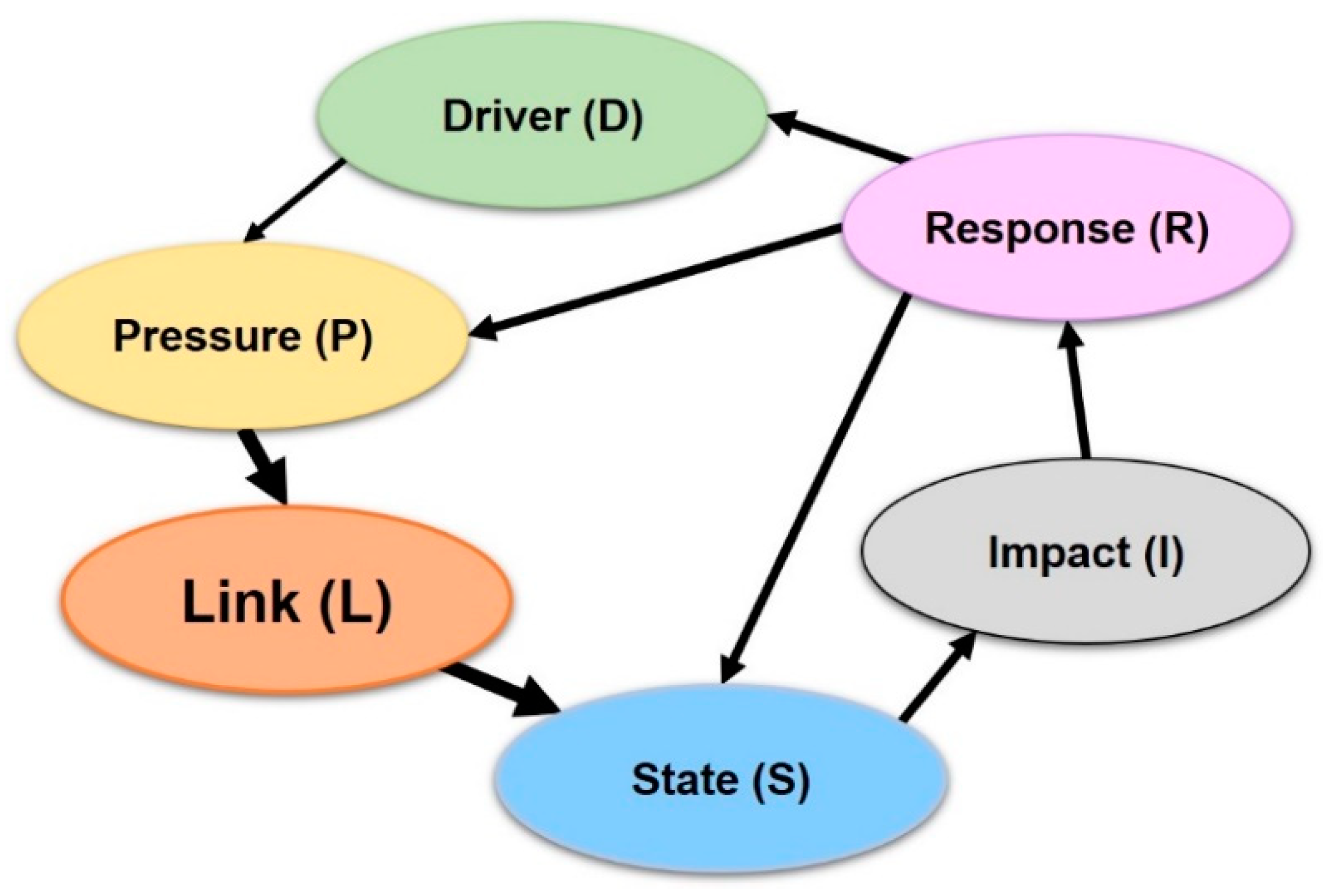
2.1. The DPLSIR Framework

The DPLSIR framework focuses on the understanding of underlying controls for the relationships between pressure and state (Figure 1). Pressure, in this study, is the amount of agricultural stress released from the agricultural system. We define the agricultural system as the zone where all agricultural activities occur, and this zone is physically defined by the zone above the bottom of the soil layer (e.g., plough layer; Figure 2). The state is the quality of the water in the hydrogeological system. The hydrogeological system is defined by the entire zone below the soil layer through which water and contaminants move (Figure 2). In the hydrogeochemical system, various biogeochemical reactions may change the concentrations of nitrate. Nitrate reduction can occur both in the soil layer and below the interface between the oxic and reduced zones, where the reduction capacity—the amount of nitrate-reducing material, such as pyrite and organic carbon—is high (Figure 2). In some places, this interface can be several meters thick, developing in an anoxic nitrate-reducing zone. Link provides information about these hydrological and biogeochemical processes that are responsible for the release, retention, and transport of water, as well as contaminants. In this study, we focused on transport of water and contaminants—how and how fast nitrate moves through the hydrogeological system. Further research may require reviewing and developing indicators to parameterize release and retention of contaminants in the hydrogeological system.

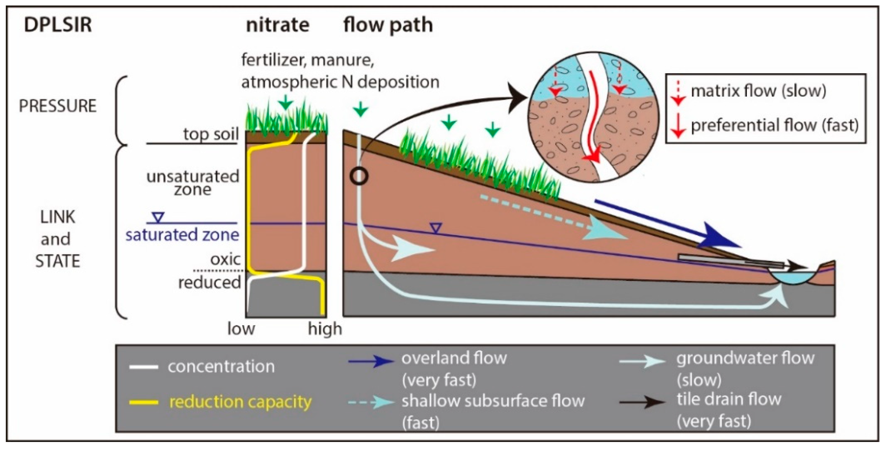
2.2. Link: Flow Pathways and Lag Time

Lag times not only quantify the delay time between the pressure stress and state response, but also reveal primary pathways of water and contaminants [28]. To recharge groundwater, water primarily flows vertically via matrix flow pathways and/or preferential flow pathways (Figure 2). This water eventually emerges in the surface water. Matrix flow is a pathway through pore spaces in the soil matrix. The lag times of matrix flow can be long (years to decades). Preferential flow is a pathway via macro-pores in soils and fractures in bedrock, bypassing a dense or less permeable matrix [29,30]. The macro porous spaces in soils can be created along root channels, soil fauna channels, cracks (i.e., freeze–thaw and wetting–drying), fissure, or soil pipes [29]. Preferential flow may be transiently active; however, it can deliver a significant quantity of contaminants with a very short time delay (hours to weeks) [31,32]. Therefore, the groundwater table and groundwater chemistry of matrix flow-dominated systems will exhibit relatively small variations and slow changes over time compared to those of preferential flow-dominated systems.

3. Materials and Methods

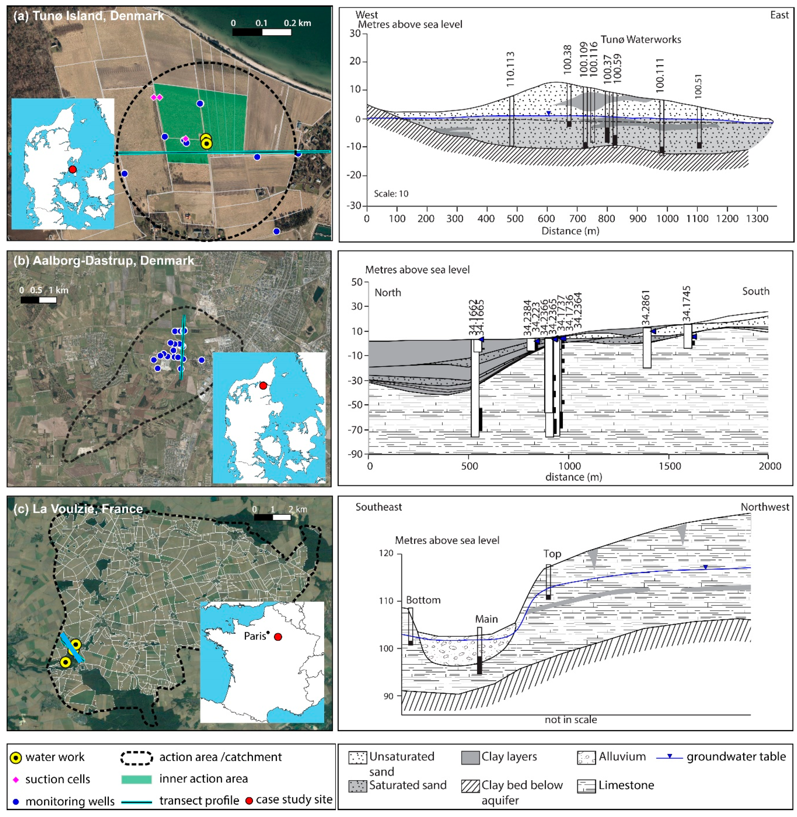
3.1. Case Study Sites

The three case study sites are intensive farming areas with groundwater-based drinking water abstraction. The first case study site is Tunø Island in Denmark (Figure 3). Tunø is a small island (area: 3.5 km2) located in the Kattegat Sea, between the North Sea and the Baltic Sea (Table 1). The main part of the subsurface of the island consists of clay-rich glacial deposits of Quaternary origin. However, in the northeastern part, where drinking water abstraction wells are located, Quaternary sandy deposits dominate the near-surface layers and contain an aquifer vulnerable to pollution (Figure 3). The groundwater is the sole source of drinking water and there is only one public water supply system, which produces approximately 10,000 m3/year of water for around 100 inhabitants and tourists.
During the 1970s, the farmers in the area around the drinking water abstraction wells changed from mixed conventional farming to intensive vegetable production, mainly the production of leeks, cabbages, and onions. This change in farming practice led to high inputs of mineral fertilizers. Since the mid-1980s, Denmark has adopted the EU directives on legislation at the national level to protect water resources, including groundwater [33]. On top of these national-level regulations, in Tunø, additional water protection plans have been implemented since 1989, mainly because high levels of nitrate were detected in the abstraction wells (≈150 mg NO3/L). From 1989, the central part of the recharging area of the abstraction wells was set as a protection zone, and in 1991, this area was extended to more than double the size to cover the major parts of the recharge area (shaded with green in Figure 3). In this inner action area as well as one field at the western border of this area, all agricultural activity has been banned, and the land has been converted to set-aside with permanent grass. In the outer part of the recharge area (total protection area), fertilizer application has been regulated to the level of the economical optimum application of nitrogen for crop production (circled area in Figure 3).
The second case study site is Aalborg-Drastrup in Denmark (Figure 3). The case study area is in northern Jutland. In the area, thin layers of glacial sand and clay till deposits of Quaternary origin overlie a fractured Maastrictian limestone reservoir. Like Tunø, groundwater is the only source of drinking water. There are well fields belonging to a public water supply system and several privately owned wells. The wells in the well field were constructed between 1958 and 2005, and the well field produces 1.5 mm3 year−1 of water distributed to around 26,000 consumers in the Aalborg area (Table 1).
The groundwater in the Aalborg-Drastrup case study area is one of the most vulnerable aquifers to nitrate pollution in Denmark because of absent or thin protecting clay layers above the chalk aquifer with a low nitrate reduction capacity in the majority of the recharging area, except in the northernmost part where thick layers of marine clay overlay the chalk (Figure 3). At the same time, there are intensive dairy and pig farms in the area, as well as arable farms. During the 1980s, the water authorities realized that the drinking water abstraction was threatened by pollution of nitrate from the agricultural production. Like Tunø, therefore, additional water protection plans were introduced. Since 2001, a series of mitigation measures were implemented, including setting a protection zone (afforestation) close to the abstraction wells, limiting nitrate leaching from zero to less than 50 mg/L of nitrate, and banning the use of pesticide.
The third case study site is the La Voulzie catchment area (drainage area: 115 km2) in France (Table 1). The catchment is located about 70 km southeast of Paris. The catchment is primarily underlain by massive limestone (Figure 3). The aquifer is one of the main resources in the water supply system (Ile-de-France) and a very important drinking water source for Paris. Eau de Paris is a public organization in charge of managing water resources for Paris. The catchment provides 20 mm3/year of water, which is equivalent to 10% of Eau de Paris’s resources, to about 400,000 people. The catchment covers 15 rural municipalities with about 100 farmers (including one organic farmer). The area is intensively used by agriculture—90% of the surface area is cultivated, 40% of which is planted with wheat (in rotation with other cereals, rape seed, and sugar beet).
The highest potential nitrogen (N) leaching was achieved in the late 1980s. The agricultural action program was launched in 1991 for the watershed (Fertimieux) to limit high concentrations of nutrients. A change in fertilizer use occurred in the late 1990s in France. This change is attributed to the beginning of environmental awareness and anticipation of the Common Agricultural Policy in 1992. The nitrate concentrations in springs, which is raw water for drinking water production, have been relatively invariant at approximately 55–70 mg NO3/L for the last two decades.

3.2. Materials

For all three study sites, three types of historical data were collected to carry out the study: (1) N surplus, (2) groundwater chemistry, and (3) groundwater age. N surplus (or N balance) is used as an environmental indicator [34,35] and it has also been applied in many EU member states including Denmark and France. Furthermore, studies have reported that N surplus is a good indicator to explain N leaching from the soil and nitrate pollution in groundwater [36,37,38,39]. Methods and input data to calculate N surplus differ among the EU member states [40]. This study compared the temporal variability of agricultural N pressure and groundwater state of each case study site, not across the sites; therefore, the methodological differences would not affect the lag time analysis. N surplus is calculated with respect to farm gate (i.e., farm gate N surplus) or to soil surface (i.e., soil surface N surplus). In this study, soil surface N surplus was the primary agricultural N pressure indicator (unit: kg N/ha/year). N surplus of each case study site was calculated according to the member state’s standard method, but in principal, soil surface N surplus calculates the differences between the annual quantity of N entering the soil and the annual quantity of N leaving the soil surface by harvested crops. For Tunø and La Voulzie, the soil surface N surplus at the relevant catchment scale was used and for the Aalborg-Drastrup site; both soil surface and farm gate N surpluses at the regional level were used. The water chemistry data were time series of nitrate in any type of water, e.g., soil pore water and groundwater. The annual average concentration of nitrate in water was used as a water quality state indicator (unit: mg NO3/L). The groundwater age data were measured or simulated values of residence times and/or water ages (unit: year). A few studies have reported chlorofluorocarbon (CFC) reduction in reduced groundwater [41,42]; hence, in this study, we only collected data of oxic and nitrate-reducing groundwater. In this study, we did not conduct extra measurements. Instead, we focused on existing data available from public databases and reports, where the data have been collected and reported following the national regulations and official guidelines at the time of collection.

3.2.1. Tunø Island, Denmark

For the Tunø study sites, input data to calculate soil surface N surplus at field scale were available; therefore, this was calculated for the period from 1975 to 2018 at the 345 m2 outer protection area. A time series of modeled annual atmospheric N deposition is publicly available at the municipality scale (2006–2016) [43]. Time series of the main crop type and fertilization were constructed for Tunø for the period of 1975–2018, at the field scale. Recent data (2010–2018) on the main crop type are available from the Ministry of Environment and Food, Danish Agricultural Agency [44], while older data from the Tunø study site were reconstructed from information on crop rotations obtained from reports [45,46]. Information on the use of fertilizer was based on reported values [46].
In Denmark, all the groundwater chemistry data are registered in the national borehole database, JUPITER, and are managed by the Geological Survey of Denmark and Greenland. The data are publicly available. Therefore, nitrate data for both Danish case study sites were obtained from JUPITER [47]. In Tunø, groundwater ages were determined at seven monitoring points using the CFC method [48].

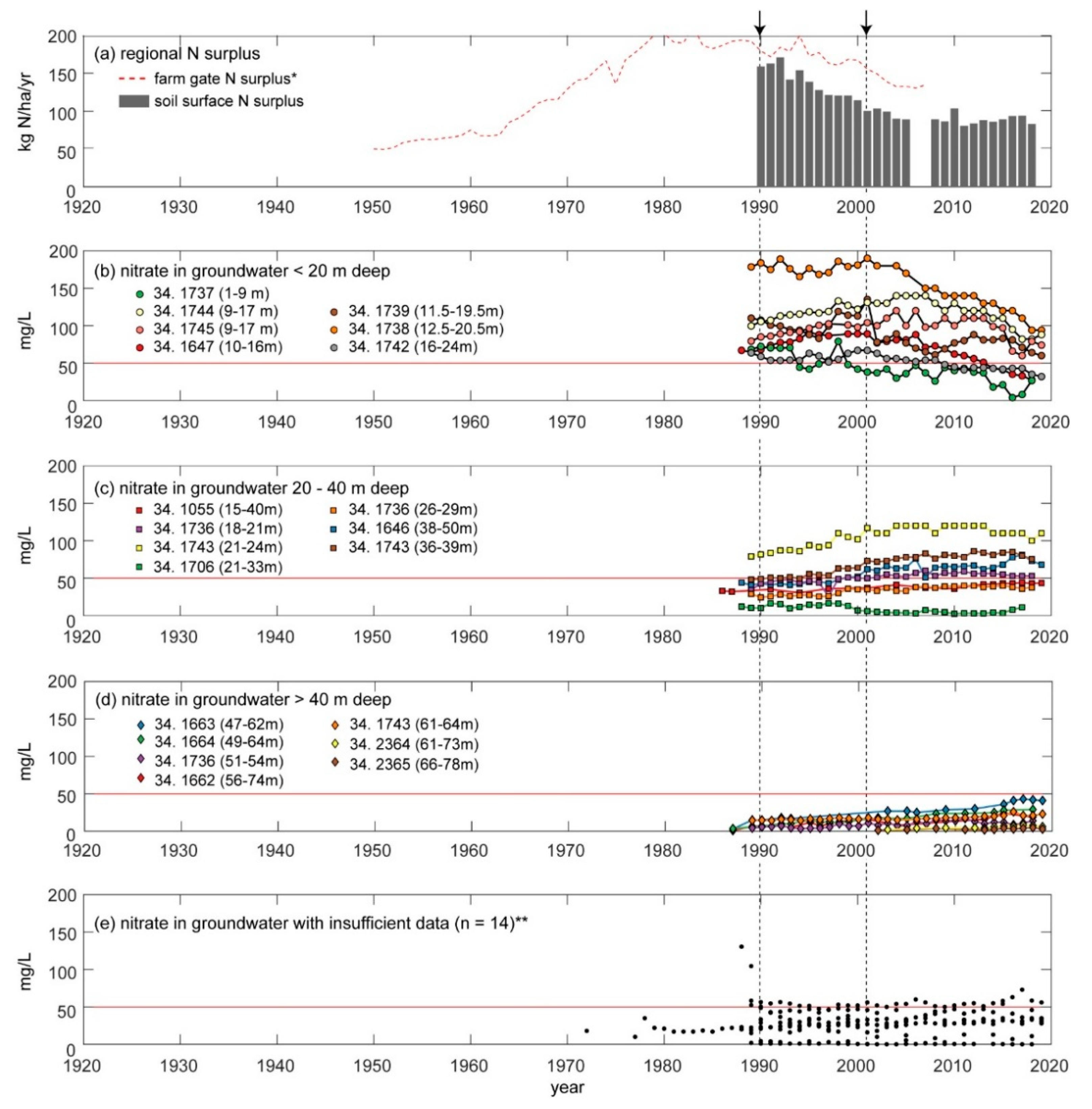
3.2.2. Aalborg-Drastrup, Denmark

Soil surface N surplus at regional scale (1990–2018) was used for the Aalbog-Drastrup site, and the detailed method and input data for the calculations are described in Windolf et al. [49]. Hansen et al. [50] reported farm gate N surplus of Denmark at the geo-region scale for the period of 1950–2007. Between 1990 to 2007, the soil surface N surplus was offset by 39 kg/ha/year on average compared to the farm gate N surplus; therefore, the soil surface N surplus for the Aalborg-Drastrup site before 1990 was estimated from the farm gate N surplus by subtracting the offset.
Within the action areas of the Aalborg-Drastrup site, monitoring wells that are part of the national groundwater monitoring program are located (Figure 3). The groundwater chemistry of these wells has been monitored regularly since 1989, and groundwater age was also determined using the CFCs method [51]. The groundwater chemistry and groundwater age data were extracted from JUPITER and the report [51].

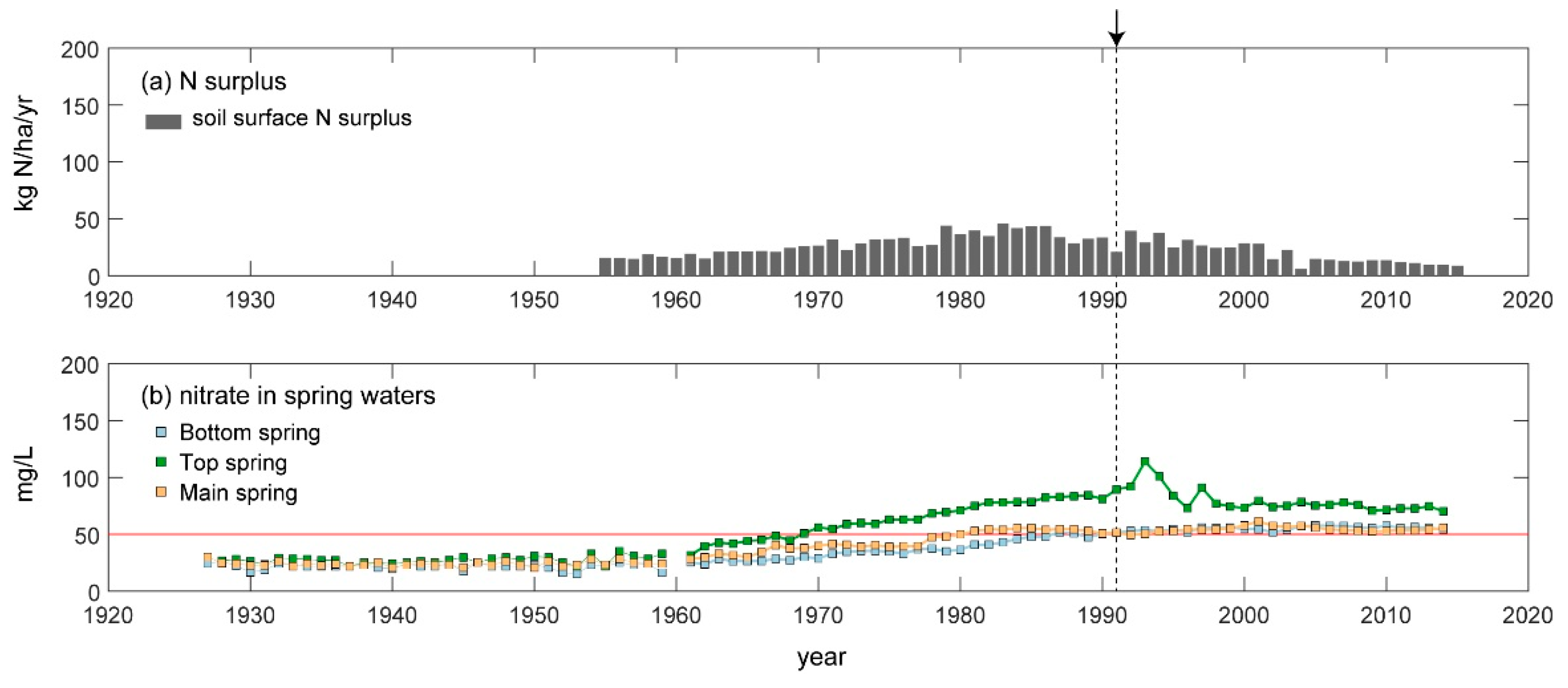
3.2.3. La Voulzie, France

For the La Voulzie site, the N surplus calculated at the University of Tours was used, with detailed description of the calculation being found in Poivert et al. [52]. The methods for N surplus calculation of Denmark and France are similar. The N surplus for the study area was extracted from an online tool available for France (Cassis-N; https://geosciences.univ-tours.fr/cassis/login) [52,53]. The concentrations of nitrate were collected by the water company “Eau de Paris” at the “La Voulzie” springs. Water chemistry has been monitored since 1927. The water chemistry was monitored 1–4 times per year before 1986 and then every month after 1986. In this study, we focused on three sampling points: top, main, and bottom springs, which are naturally under pressure (Figure 3). The main spring is the primary source of drinking water produced at the water company, and its volume represents 45% of the total volume of the drinking water production. The top spring collects water in the top limestone layer over the thin clay layer that is situated about 5 m below the land surface (Figure 3). The bottom spring and the main spring collect water in a ≈10 m thick limestone layer situated below the thin clay layer (Figure 3). The average depth of the three wells is 14 m, and the groundwater table at the main spring is 1 m below the land surface.

3.3. Lag Time Estimations

The lag time between soil surface N surplus (x) and annual average concentrations of nitrate in water (y) was calculated using a cross-correlation method (CCF) using a correlation coefficient function of Matlab. The CCF method assumes a linear dependency of two variables, i.e., soil N surplus and nitrate concentrations, and the lag time is the time difference between a soil surface N surplus peak and a nitrate concentration peak. The lag times were calculated for a range of time lags (k; year); for example, a correlation between x at time t and y at time t + k was calculated. The range of k was from 0 to 50 years. The CCF provides two main results: (1) the strength of the correlations between x and y (correlation coefficient, r), and (2) the significance of the correlation (p-value). The strength of the correlation varies between 0 (no correlation) and ±1 (strong correlation). The highest r and statistically significant k-year was defined as lag time.

4. Results

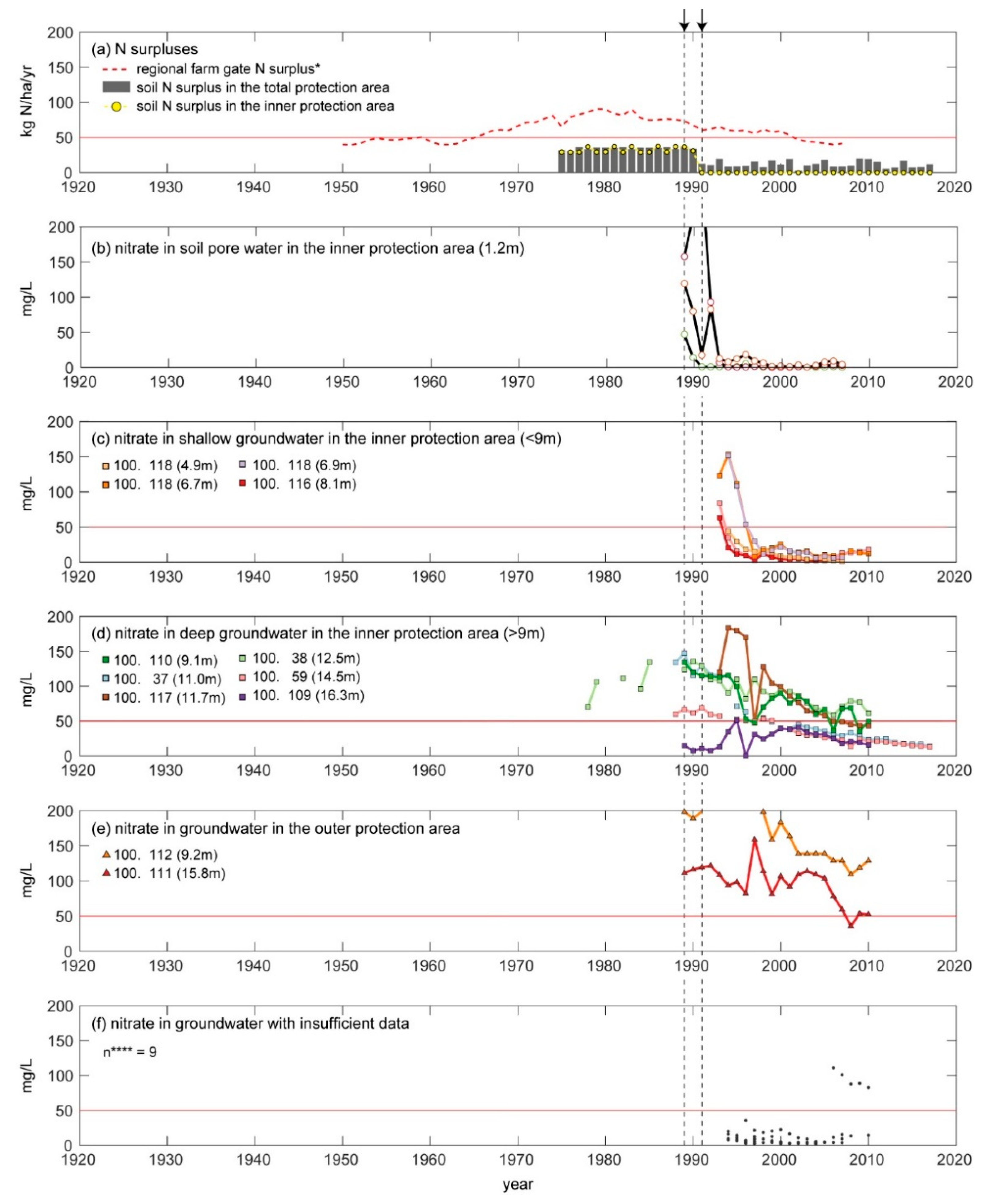
4.1. Time-Series of Surface Soil N Surplus and Water Chemistry

Figure 4a shows the soil surface N surplus at the field scale calculated in this study and the farm gate N surplus at the geo-regional scale of Tunø Island [50]. When the protection plans were first introduced, the soil N surplus at the field scale from the agricultural system in the inner action area decreased to the input from the atmospheric deposition, as no other input and no harvest occurred from those fields (yellow circles in Figure 4a). No manure was applied in both the inner and the outer protection area. The soil N surplus at the field scale of the total protection area was averaged at 35 kg N/ha/year before the protection plan period (1975–1990) and was averaged 12 kg N/ha/year after that (1991–2018; gray bars in Figure 4a). The farm gate N surplus at the geo-regional scale peaked around the mid-80s (≈90 kg N/ha/year) and has decreased since then (≈40 kg N/ha/year), which is explained by the effects of the national N regulations [50]. The farm gate N surplus at the geo-regional scale was much higher than the soil surface N surplus at the field scale (Figure 4a). The discrepancy may be because of stricter regulations implemented at the local scale.
As a result of the intensified agriculture, the nitrate concentrations in groundwater and drinking water increased up to >100 mg NO3/L in the 1980s (Figure 4d). As the protection plans set in, nitrate concentrations in soil pore water and groundwater started to respond. The annual average concentrations of nitrate of soil pore water (1.2 m) in the inner protection area decreased nearly to zero almost instantaneously (Figure 4b). The annual average concentration of nitrate in shallow groundwater (<9 m deep) started to decrease a few years after the protection plans (Figure 4c) and those in the deeper groundwater slowly decreased down to ≈10 mg NO3/L over the past two decades (Figure 4d). The annual average concentration of nitrate of groundwater in the outer protection area also decreased over time, but the concentrations were still relatively high (50–100 mg NO3/L; Figure 4e).
In terms of Aalborg-Drastrup, the two regional N surpluses, the soil surface and the farm gate, are shown in Figure 5a. These regional scale data do not precisely represent the impact of the mitigation measured implemented at the local level; however, they may be a good proxy to estimate the overall trend of agricultural N pressure of the study area. The soil surface N surplus decreased from 159 kg N/ha/year in 1990 to 83 kg N/ha/year in 2018. In this period, the annual input of manure was at a stable level of approximately 104 kg N/ha/year, while the input of mineral fertilizer decreased from 139 to 70 kg N/ha/year, as mitigation measures for higher utilization of N in manure were implemented, e.g., higher manure storage capacity and increased manure application in spring and summer rather than in the period with higher leaching in autumn and winter.
In the monitoring site of the Aalborg-Drastrup (Figure 3), the annual average concentrations of nitrate of groundwater varied within a wide range (1–200 mg NO3/L), and their temporal variability also was heterogeneous (Figure 5b–e). The groundwater in shallower depth (filter interval < 20 m) showed the greatest temporal variability, and the nitrate concentrations showed peaks around 2000–2010 and decreased over time (Figure 5b). The groundwater measured between 20–40 m intervals showed relatively damped responses (Figure 5c). In some monitoring points, the nitrate concentrations peaked around 2010 and slowly decreased over the past 10 years (e.g., 34. 1743 in Figure 5c). While nitrate of groundwater in the deeper intervals (>40 m) were relatively low, i.e., <10 mg NO3/L, in some groundwater wells, the concentrations continuously increased over the entire monitoring period (e.g., 34. 1663 in Figure 5d). At 14 monitoring points, either the groundwater was in reduced conditions, the nitrate concentrations were temporally invariant, or the nitrate concentrations showed only increasing trends (Figure 5f).
In the La Voulzie catchment area, the soil surface N surplus at the catchment scale was highest around the mid-80s (≈77 kg N/ha/year) and then decreased to ≈55 kg N/ha/year around 1990 (Figure 6a). Over the past 30 years, the soil surface N surplus ranged between 15 and 66 kg N/ha/year (Figure 6a). The groundwater chemistry has been monitored since 1927. Until the 1960s, the annual average concentrations of nitrate of groundwater and spring waters ranged between 20 and 25 mg NO3/L, but the level continuously increased up to 50–110 mg NO3/L until 1993 (Figure 6b). The nitrate concentrations of the top spring decreased back to approximately 74 mg NO3/L around 2000 and then were temporally invariant for the last 20 years at this level (Figure 6b). Those of the main and bottom springs also were relatively stable at around 55 mg NO3/L for the last 30 years (Figure 6b). The monthly data revealed that the nitrate concentrations of all three springs did not show any seasonality—standard deviations of all the nitrate measurements between 2000 and 2014 were 2.8 (top spring), 2.2 (main spring), and 1.8 (bottom spring).

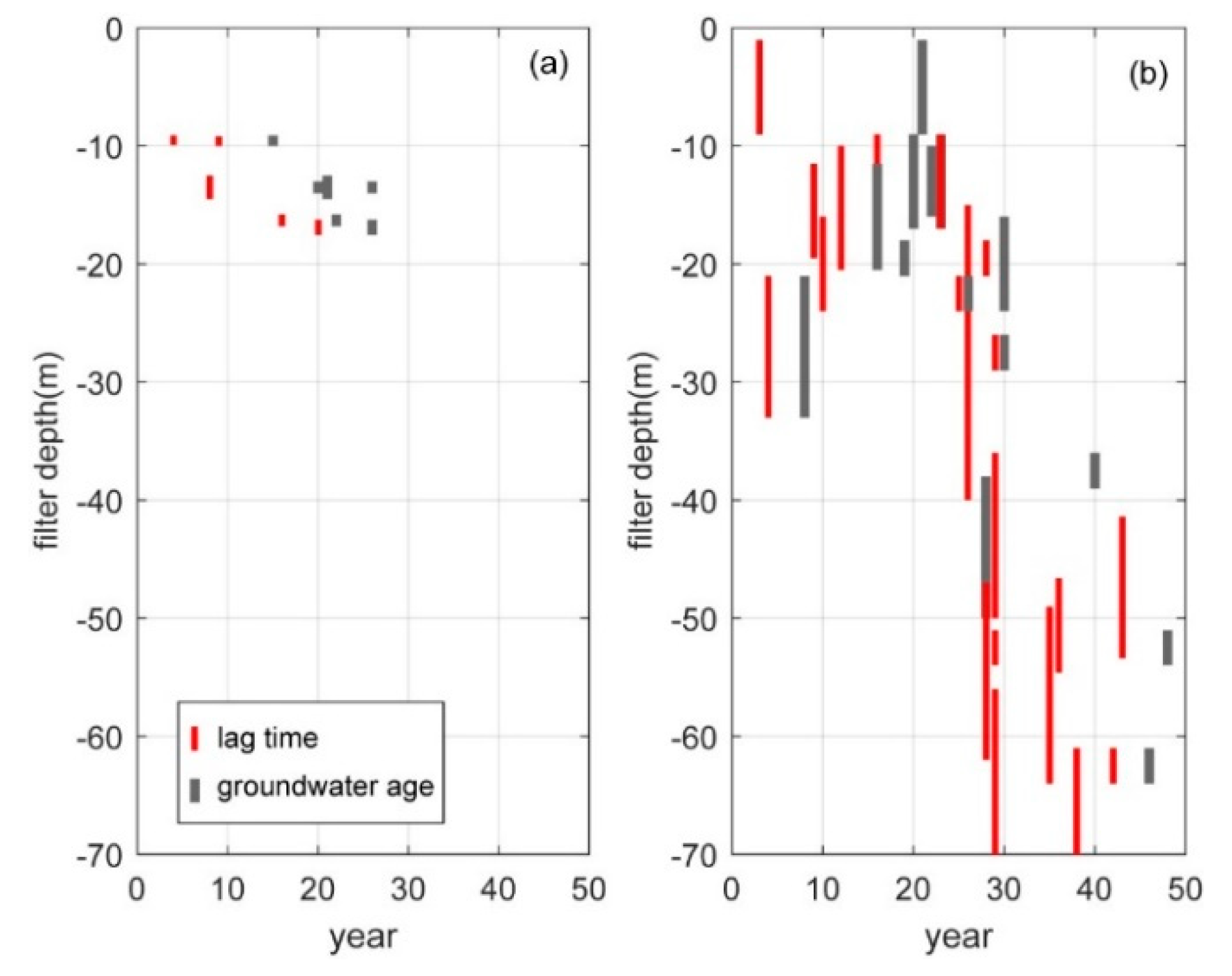
4.2. Lag Time between Agricultural Pressure and Groundwater Quality State

Table 2 summarizes the results of the lag time analysis of the case study sites and water chemistry. For the Tunø site, at the 15 points with statistically significant results, the soil surface N surplus showed strong correlation with the annual average concentrations of nitrate in water. For example, except for the deepest groundwater, the correlation coefficients were higher than 0.76 and the results were statistically significant (p < 0.005) in all the cases (Table 2). For the deepest well (monitoring point 100. 109), which is in nitrate-reducing conditions, the correlation coefficient was 0.53, and it was statistically significant (p < 0.05; Table 2). The lag times progressively increased with an increasing depth (Figure 7a and Table 2). For instance, the soil pore water measured at 1.2 m below the land surface and showed lag times of 0–2 years, while the deep wells (deeper than 10 m) showed lag times of 5–16 years.
In the Aalborg-Drastrup site, at 21 of the 35 monitoring points, the nitrate concentrations in groundwater showed significant correlations with the surface soil N surplus at the regional scale (Table 2). Except for one monitoring point (34. 1745 in Table 2), the correlation coefficients were higher than 0.73 and they were statistically significant (p < 0.005). Like Tunø, the lag times roughly increased with an increasing depth; however, they showed a greater variability (Figure 7 and Table 2). For example, at the filter interval between 21–33 m (34. 1706), 4 years of lag year was estimated. In the deeper part of the groundwater (>40 m), the lag times also varied between 29 to 42 years.
In the La Voulzie catchment area, the soil surface N surplus and the annual average concentrations of nitrate of all three springs showed strong (r = 0.70–0.83) and statistically significant correlations (p < 0.005). The lag times estimated for the top, main, and bottom springs were 8, 15, and 24 years (Table 2).

4.3. Groundwater Age

For the Danish case study sites, groundwater age data were collected to compare them with the lag time analysis results. In Tunø, groundwater age data are available at five monitoring points in the inner action area and at two points outside the inner action area [48]. Like the lag time, the groundwater age of the Tunø groundwater linearly increased with an increasing depth (Figure 7a). However, the groundwater ages for the same depth were 6–14 years longer than the lag times estimated in this study (Figure 7a). In the Aalborg-Drastrup site, like lag times, groundwater ages varied widely with depth (Figure 7b). For instance, young groundwater (<10 years old) was found at 21–33 m below the land surface, while old groundwater (≈20 years old) was found in the near surface groundwater (Figure 7b). Like in Tunø, the groundwater ages were relatively longer than the lag times calculated in this study.

5. Discussion

5.1. Methodological Evaluation of the Lag Time Estimation and Data Requirements

Lag times may be one of the key pieces of information for developing water protection programs and setting achievable goals [54,55,56,57]. Various models have been developed to estimate the lag times between mitigation measures and the water quality changes [55,56,57,58,59]. Most models are process-based and provide comprehensive views of the system. Modelling is applicable both data-rich and data-poor sites [55]. However, these models often require scientific and technical training to use them. Therefore, these tools may not be readily available for many stakeholders. Furthermore, such models are often based on various assumptions; therefore, building trust on the modeling results may require considerable efforts. Studies have reported that involving the stakeholders in the modelling processes improve the acceptable of the modeling results [55]. This study selected the CCF analysis, which is based on direct measurements. This method is a simple, intuitive, and easy-to-use method for the stakeholders. Such measurement-based methods require good quality and quantity of data [55], and we also found that the CCF analysis may provide meaningful and statistically significant results if the following conditions are satisfied.
First, continuous, long-term monitoring data on both the agricultural pressure and groundwater state should be available. Obviously, the time series of the data must be sufficiently long to document the cause and effect relations between the pressure and state. For example, in La Voulzie, both agricultural pressure and groundwater state data were available for nearly a century and could thus fully cover the changes in agricultural pressure and the groundwater state responses (Figure 6). For the two Danish sites, regional long-term farm gate N surplus data indicated the trends in agricultural pressure, confirmed by overlapping more recent soil surface balances. These long-term data allowed statistical analysis and the results of the CCF analysis were statistically significant. However, links between regional N-surplus pressure data and effects on resulting levels of nitrate leaching should be subject to further research [40]. Supplementary analyses of more detailed historical, agricultural pressure data [60] for the local Parishes covering both of the two Danish sites showed that the farm gate N surplus levels for both Tunø (represented by the Parish of Tunø) and Aalborg-Drastrup (represented by the two Parishes of Dall and Navling) were about 20% and 10% lower than the regional balances shown in Figure 4 and Figure 5, respectively, but with similar decadal trends. This confirms the validity of the current analyses. Furthermore, the local data confirmed the high decrease in N surplus pressure for Tunø after the 1980s, as well as historical trends back in time similar to the regional results. For Aalborg-Drastrup, the agricultural pressure according to local agricultural N-surplus followed the regional trend after 1980 but was significantly higher before 1980. Thereby, the value of localized data about links between agricultural pressures and lag time in groundwater quality was supported.
Second, particularly for evaluating the effectiveness of the mitigation measures, the time series should capture the changes in pressure and state. For instance, in Tunø, at some sampling points, groundwater monitoring had started a few years after the protection plans were implemented (Figure 4f). The nitrate concentrations in those wells already decreased below 10 mg NO3/L, and they were relatively invariant over time. With these time series, the CCF analysis cannot produce statistically meaningful results.
Third, in cases of the groundwater state, only oxic groundwater should be considered because nitrate is redox-sensitive. In nitrate-reducing and/or -reduced conditions, nitrate concentrations decrease not only because of the changes in the inputs from the agricultural system, but also because of biogeochemical reactions (denitrification to gaseous N compounds) in the subsurface. If the denitrification reactions dominantly control the nitrate concentrations in groundwater, the correlations between the agricultural pressure and groundwater state might not be strong or statistically significant. For example, in Tunø, the deepest groundwater (100. 109) was nitrate-reducing, the CCF analysis estimated weak correlations, and one of the pressure indicators showed an insignificant result (Table 2). These results are attributed to its nitrate-reducing condition. In this well, oxygen was nearly depleted, but its nitrate concentrations were much lower (approximately 25 mg NO3/L) than the overlying part of the groundwater (44–170 mg NO3/L), indicating that nitrate had begun to be reduced. Therefore, to evaluate the effects of agricultural activities, including mitigation measures, on the groundwater quality, the role of nitrate reduction reactions in the hydrogeological system should be excluded.

5.2. Hydrogeological Control of Lag Times

The hydrological system determines the pathways between a source (i.e., agricultural soil) and a sink (i.e., groundwater) and the travel speed of the contaminants through the pathways. All the hydrogeological systems, however, have complex networks of flow pathways, and this complexity has been a major challenge in communication among stakeholders, water authorities, and scientists. To develop a water protection program with local stakeholders, it may be more important to identify the most dominant pathways of water and nitrate transport, rather than to fully understand the complexity of the hydrogeological system. By targeting the primary pathways, the efficiency of the mitigation measures may be increased [19,61]. The main role of the link indicators is to reveal the primary pathways of the site so that the stakeholders can develop action plans and set achievable goals. Tunø is a sandy aquifer underlain by Quaternary glacial deposits, where heterogeneous geology and flow pathway network are expected. However, our data showed that lag times and groundwater ages linearly increased with an increasing depth at this site (Figure 7a). These results imply that the signals of the agricultural pressure are propagated downward, predominantly via matrix flow (i.e., diffusion and dispersion through the porous medium) to groundwater. In a matrix flow-dominated system, the groundwater state may respond to the agricultural pressure slowly, which is consistent with the relatively long lag times of the Tunø site.
The Aalborg-Drastrup site is underlain by limestone. Limestone aquifers are also well known for their complexity and anisotropy of flow networks because both matrix flow via porous medium and preferential flow via fractures play a key role in transporting water and contaminants [62]. This complexity may explain why the lag time and residence times heterogeneously varied with depth. When preferential flow via large fractures is the dominant pathway, the agricultural pressure signals will rapidly propagate to groundwater, and consequently young groundwater and short lag times can be found at deep depths in this case (Figure 7b). Conversely if matrix flow via porous medium or macroscale fractures plays a more important role in delivering water and nitrate, the groundwater state responses will be significantly delayed. At the Aalborg-Drastrup site, we observed both patterns and these observations imply that both pathways may be active. In this case study site, mitigation measures that target rapid (i.e., preferential flow) and slow (i.e., matrix flow) pathways will be needed.
La Voulzie is also underlain by limestone. A previous study using multiple tracers in this area revealed that, at this site, nitrate transport mainly occurs through matrix flow on a long-term timescale [63]. Consistent with this, the lag times of nitrate were 8–24 years (Table 2) and the monthly water chemistry data showed no seasonal variations. At this site, therefore, a long-term water protection program will be necessary. Furthermore, the results also show that the lag time variability among the springs may be explained by the hydrogeological structure of the subsurface. At the top spring, the estimated lag time is shorter than those of the other two springs. These differences may be because the top spring is located above the relatively impermeable clay layer (Figure 3), while the other two are located below it. Therefore, the top spring may receive water that circulates only within the top limestone layer. In sum, we conclude that the link indicators may be useful for better understanding of how water and nitrate move through the hydrological system and selecting the best mitigation measures. The underlying hydrogeology is the primary control of the relations between the agricultural pressure and groundwater state. Therefore, the hydrogeological system should be well-characterized in the context of the objectives and the spatial and temporal scales of the water protection programs.

5.3. Link Indicators: Groundwater Age vs. Lag Time

The time lags between pressure and state can also be estimated through groundwater age measurements using environmental tracers such as CFCs, 3H/3He, and noble gases (Ar, He, Kr, Ne, and Xe) if the contaminant is highly soluble [64,65,66,67,68]. Nitrate is primarily transported as solutes and behaves conservatively in the oxic zone; therefore, the groundwater age may be a useful indicator for estimating the time lag of groundwater state responses. Indeed, previous studies of groundwater ages and groundwater chemistry have successfully documented the changes of nitrate concentrations in groundwater chemistry as responses to the changes of regulations or agricultural practices at decadal scale [64,65,66,67,68].
Our results show that the lag times estimated using the statistical CCF method were shorter than the measured CFC groundwater ages in Tunø. Such differences could be attributed to uncertainties associated with each measurement; however, in principle, lag time and groundwater age represent two different hydrological timescales. Lag time measures the time difference between a pressure peak and a state peak; therefore, it quantifies how fast a water parcel or an input signal moves through a groundwater system [69]. In other words, lag time is transit time. Comparatively, groundwater age is the mean residence time of the water; therefore, it is related to water mass movement and the volume of the groundwater. If the lengths of pathways of a hydrogeological system are identical, its lag time is half of the mean residence time [70]. However, such hydrogeological systems do not exist. The lengths of pathways are greatly different, even for a relatively homogeneous system; therefore, some signals can propagate through the system via short pathways (i.e., short lag time), while the rest take longer pathways (i.e., long residence time). In other words, water can be contaminated quickly, but it will take much longer to remediate it.
When the lag time and groundwater age are used as link indicators in communications with stakeholders, it is important to make a distinction between these two link indicators and to assess the limitations of each indicator. The CCF method is a statistical analysis tool and it does not provide process-based understandings of the lag time between the agricultural pressure and groundwater state. The lag time is controlled by the interplay between hydrological and biogeochemical processes [71], which potentially results in an unclear correlation between the agricultural pressure and groundwater state and in highly uncertain estimations of lag times. Therefore, lag time results should be carefully examined on the basis of good understandings of the hydrogeological system.
The groundwater age is the mean age of the exiting waters at the monitoring point in the aquifer, and it does not provide information about the age distribution by itself. Information about the age distribution, however, may be critical to identifying the sources and timing of the contamination [72] and to estimating the time span of the water protection plans. If the ages of a water body show a normal distribution, for example, then it will take twice as long as the mean residence time to replace all the waters in the water body. However, it is well documented that groundwater is a mixture of waters with vastly different ages, often displaying a skewed distribution with a long tail or a bimodal distribution (e.g., [72,73]). Several models and multiple tracers methods are available to estimate the distribution of water ages, and different methods may predict different distribution patterns (e.g., [66,72,74]). Therefore, when using the groundwater age as a link indicator, the age distribution and limitations associated with the employed method should be provided.

5.4. Lag Time as a Criterion for the Selection of Pressure and State Indicators

Because different stakeholders have different interests, they focus on different aspects of drinking water protection plans. For example, farmers may be interested in the effects of the implemented measures on their fields. For the field level evaluation, the spatial scale of the agricultural N pressure (i.e., N surplus) will be essential. For example, the farm gate N surplus at the geo-regional scale of the Tunø case study site did not show the effects of the local mitigation measures, whereas soil surface N surplus at the field scale showed instantaneous reduction (Figure 4a). Indeed, many EU member states have adopted N surplus (or N balance, N budget) at the field level as an advisory or regulatory tool [40]. For instance, the Danish agriculture and Food Council works on a fertilizer planning system that precisely calculates the soil surface N balance and surplus on individual fields of the farmer, giving the farmer the opportunity to take this soil surface N surplus into account when the farmer plans the application of mineral and manure nitrogen to his or her crops. Therefore, farmers can readily calculate N surplus at the field scale.
In combination with the soil surface N surplus, soil pore water chemistry may be useful to evaluate the effects of mitigation measures at the field scale because of its short lag time. Our results show that nitrate in soil pore water responds to the agricultural pressure almost instantaneously (lag time between 0 and 2 years; Table 2) and the strength of their correlation was strong (0.75–0.85; Table 2) in Tunø. Indeed, the soil pore water chemistry, which is generally referred to as N leaching, is one of the most widely monitored parameters for scientific, monitoring, and regulatory purposes in order to quantify N losses from the agricultural system to the hydrogeological system [36,75,76,77]. Several methods have been developed, and the advantages and limitations of each method are well documented (e.g., [75,78,79]). Because of the spatial heterogeneity and temporal variability of soil pore water chemistry, establishing monitoring networks and obtaining representative values for N leaching will be costly and labor-intensive; however, nitrate in soil pore water collected below the root zone directly measures the amount of nitrate loss after the complex interplay between agricultural and biogeochemical N cycles in the soil layer. Furthermore, farmers or citizens can be part of the monitoring procedure; therefore, this may contribute to increasing the transparency of the indicator. We strongly recommend developing a sampling protocol to account for the spatial and temporal variability of the soil pore water chemistry that can document the link between N surplus and nitrate concentration in soil pore water.
On the other hand, water companies and authorities may be more interested in the changes in the quality of drinking water resources that likely integrate signals from the entire catchment or recharging area. In order to do this, N surplus may be calculated for the area of interest, i.e., catchment or recharging area, and nitrate concentrations in oxic groundwater can be used as a water quality state indicator. To specifically evaluate the effects of the mitigation measures, oxic groundwater should be focused upon because the effects of naturally occurring N reduction reactions are negligible in oxic conditions. In addition, our results of all three case study sites showed that the lag times generally increased with an increasing distance from the N source (e.g., depth or flow pathways). Therefore, oxic groundwater close to the N source may be most effective for rapid communication with the stakeholders. It is equally important to select representative locations for oxic groundwater monitoring because the groundwater chemistry and lag time responses can be spatially heterogenous. Therefore, monitoring programs should be carefully established to document the spatial and temporal variability of the site.

6. Conclusions

This study investigated lag times as a link indicator to better understand the cause–effect relations between agricultural N pressure and groundwater quality state using data from the three case study sites. We showed that the cross-correlation (CCF) analysis of soil surface N surplus and annual average concentrations of nitrate in water can be a simple and useful method to determine the lag times between agricultural N pressure and groundwater quality state if long-term pressure and state data are available. Furthermore, the spatial patterns of lag time distribution revealed the dominant pathways of water and nitrate, which then provide valuable information for the selection of mitigation measures. Groundwater age is another useful link indicator to estimate the timescale of the water quality state responses to the agricultural pressure, particularly in data-limited circumstances. However, lag time represents transit time while groundwater age measures residence time; thus, these two should be distinguished in communication with the stakeholders.
Altogether, we concluded that the link indicators investigated under the DPLSIR framework can illustrate some of the potential for enhancing the communication of uncertainties and complexity between the agricultural pressure and groundwater state. When dealing with groundwater and agriculture-related issues, the link between the pressure and state is important for the responses (in terms of measures and policies) adopted by authorities that are to be accepted and used by farmers. If there is a common understanding of the link among the stakeholders, then decisions and water protection plans might be easier to implement. Knowledge exchange on the link between decision-takers (farmers) and decision-makers (policymakers and water work) should be one of the first steps when developing water protection plans in the future.

Author Contributions

For research articles with several authors: conceptualization, H.K., A.H., N.S., and B.H.; methodology, H.K. and A.H.; validation, H.K., N.S., and A.H.; formal analysis, H.K., N.S., and A.H.; data curation, H.K., N.S., I.M., G.B.-M., and A.H.; writing—original draft preparation, H.K.; writing—review and editing, H.K., N.S., I.M., M.G., G.B.-M., T.D., and B.H.; visualization, H.K.; supervision, B.H.; funding acquisition, B.H. All authors have read and agreed to the published version of the manuscript.

Funding

This project has received funding from the European Union’s Horizon 2020 research and innovation program under grant agreement no. 727984.

Acknowledgments

We would like to thank the reviewers for the comments. This paper has been produced in the context of the project Fairway (farm system management and governance for producing good water quality for drinking water supplies; grant no. 727984). The authors thank “Eau de Paris” for providing ground state data of the La Voulzie catchment. The authors also thank Lærke Thorling, who took part in collecting the original Tunø data, for discussing the Tunø case study site.

Conflicts of Interest

The authors declare no conflict of interest.

References

  1. WHO. WHO Guidelines for Drinking-Water Quality; World Health Organization: Geneva, Switzerland, 2011; Volume 38. [Google Scholar]
  2. Knobeloch, L.; Salna, B.; Hogan, A.; Postle, J.; Anderson, H. Blue babies and nitrate-contaminated well water. Environ. Health Perspect. 2000, 108, 675–678. [Google Scholar] [CrossRef] [PubMed]
  3. Ward, M.; Jones, R.; Brender, J.; de Kok, T.; Weyer, P.; Nolan, B.; Villanueva, C.; van Breda, S. Drinking water nitrate and human health: An updated review. Int. J. Environ. Res. Public Health 2018, 15, 1557. [Google Scholar] [CrossRef] [PubMed] [Green Version]
  4. Espejo-Herrera, N.; Gràcia-Lavedan, E.; Boldo, E.; Aragonés, N.; Pérez-Gómez, B.; Pollán, M.; Molina, A.J.; Fernández, T.; Martín, V.; La Vecchia, C.; et al. Colorectal cancer risk and nitrate exposure through drinking water and diet. Int. J. Cancer 2016, 139, 334–346. [Google Scholar] [CrossRef] [PubMed]
  5. Schullehner, J.; Hansen, B.; Thygesen, M.; Pedersen, C.B.; Sigsgaard, T. Nitrate in drinking water and colorectal cancer risk: A nationwide population-based cohort study. Int. J. Cancer 2018, 143, 73–79. [Google Scholar] [CrossRef]
  6. Temkin, A.; Evans, S.; Manidis, T.; Campbell, C.; Naidenko, O.V. Exposure-based assessment and economic valuation of adverse birth outcomes and cancer risk due to nitrate in United States drinking water. Environ. Res. 2019, 176, 108442. [Google Scholar] [CrossRef]
  7. European Environmental Agency. Main Drinking Water Problems. Available online: https://www.eea.europa.eu/data-and-maps/figures/main-drinking-water-problems (accessed on 20 May 2020).
  8. Glavan, M.; Železnikar, Š.; Velthof, G.; Boekhold, S.; Langaas, S.; Pintar, M. How to enhance the role of science in European Union policy making and implementation: The case of agricultural impacts on drinking water quality. Water 2019, 11, 492. [Google Scholar] [CrossRef] [Green Version]
  9. European Commission. Framework for Action for the Management of Small Drinking Water Supplies; European Union: Brussel, Belgium, 2014. [Google Scholar]
  10. European Commission Synthesis Report on the Quality of Drinking Water in the EU Examining the Member States’ Reports for the Period 2008–2010 under Directive 98/83/EC EN; European Union: Brussel, Belgium, 2014.
  11. OECD. OECD Principles on Water Governance. Available online: https://www.oecd.org/governance/oecd-principles-on-water-governance.htm (accessed on 20 May 2020).
  12. Young, S.; Plummer, R.; FitzGibbon, J. What can we learn from exemplary groundwater protection programs? Can. Water Resour. J. 2009, 34, 61–78. [Google Scholar] [CrossRef]
  13. De Loë, R.C.; Di Giantomasso, S.E.; Kreutzwiser, R.D. Local capacity for groundwater protection in ontario. Environ. Manag. 2002, 29, 217–233. [Google Scholar] [CrossRef]
  14. Ivey, J.L.; de Loë, R.; Kreutzwiser, R.; Ferreyra, C. An institutional perspective on local capacity for source water protection. Geoforum 2006, 37, 944–957. [Google Scholar] [CrossRef]
  15. Graversgaard, M.; Hedelin, B.; Smith, L.; Gertz, F.; Højberg, A.L.; Langford, J.; Martinez, G.; Mostert, E.; Ptak, E.; Peterson, H.; et al. Opportunities and barriers for water co-governance—A critical analysis of seven cases of diffuse water pollution from agriculture in Europe, Australia and North America. Sustainability 2018, 10, 1634. [Google Scholar] [CrossRef] [Green Version]
  16. Serrat-Capdevila, A.; Valdes, J.; Gupta, H. Decision support systems in water resources planning and management: Stakeholder participation and the sustainable path to science-based decision making. In Efficient Decision Support Systems—Practice and Challenges from Current to Future; InTechOpen: London, UK, 2011; pp. 1–16. [Google Scholar]
  17. Jacobs, K.; Lebel, L.; Buizer, J.; Addams, L.; Matson, P.; McCullough, E.; Garden, P.; Saliba, G.; Finan, T. Linking knowledge with action in the pursuit of sustainable water-resources management. Proc. Natl. Acad. Sci. USA 2016, 113, 4591–4596. [Google Scholar] [CrossRef] [PubMed] [Green Version]
  18. Van Meter, K.J.; Basu, N.B. Time lags in watershed-scale nutrient transport: An exploration of dominant controls. Environ. Res. Lett. 2017, 12, 084017. [Google Scholar] [CrossRef]
  19. Meals, D.W.; Dressing, S.A.; Davenport, T.E. Lag time in water quality response to best management practices: A review. J. Environ. Qual. 2010, 39, 85–96. [Google Scholar] [CrossRef]
  20. European Environment Agency (EEA). EEA Glossary. Available online: https://www.eea.europa.eu/help/glossary/eea-glossary/dpsir (accessed on 1 May 2020).
  21. Bagordo, F.; Migoni, D.; Grassi, T.; Serio, F.; Idolo, A.; Guido, M.; Zaccarelli, N.; Fanizzi, F.P.; De Donno, A. Using the DPSIR framework to identify factors influencing the quality of groundwater in Grecìa Salentina (Puglia, Italy). Rend. Lincei 2016, 27, 113–125. [Google Scholar] [CrossRef]
  22. Mattas, C.; Voudouris, K.; Panagopoulos, A. Integrated groundwater resources management using the DPSIR approach in a GIS environment context: A case study from the Gallikos river basin, North Greece. Water 2014, 6, 1043–1068. [Google Scholar] [CrossRef] [Green Version]
  23. Song, X.; Frostell, B. The DPSIR framework and a pressure-oriented water quality monitoring approach to ecological river restoration. Water 2012, 4, 670–682. [Google Scholar] [CrossRef] [Green Version]
  24. Rekolainen, S.; Kämäri, J.; Hiltunen, M.; Saloranta, T.M. A conceptual framework for identifying the need and role of models in the implementation of the water framework directive. Int. J. River Basin Manag. 2003, 1, 347–352. [Google Scholar] [CrossRef]
  25. Carr, E.R.; Wingard, P.M.; Yorty, S.C.; Thompson, M.C.; Jensen, N.K.; Roberson, J. Applying DPSIR to sustainable development. Int. J. Sustain. Dev. World Ecol. 2007, 14, 543–555. [Google Scholar] [CrossRef]
  26. Smeets, E.; Weterings, R. Environmental Indicators: Typology and Overview; Technical Report No. 25; European Environment Agency: Copenhagen, Denmark, 1999. [Google Scholar]
  27. Gabrielsen, P.; Bosch, P. Environmental Indicators: Typology and Use in Reporting; European Environment Agency: Copenhagen, Denmark, 2003. [Google Scholar]
  28. Koh, E.-H.; Lee, E.; Kaown, D.; Green, C.T.; Koh, D.-C.; Lee, K.-K.; Lee, S.H. Comparison of groundwater age models for assessing nitrate loading, transport pathways, and management options in a complex aquifer system. Hydrol. Process. 2018, 32, 923–938. [Google Scholar] [CrossRef]
  29. Beven, K.; Germann, P. Macropores and water flow in soils. Water Resour. Res. 1982, 18, 1311–1325. [Google Scholar] [CrossRef] [Green Version]
  30. Hendrickx, J.M.H.; Flury, M. Uniform and preferential flow mechanisms in the vadose zone. In Conceptual Models of Flow and Transport in the Fractured Vadose Zone; National Academies Press: Washington, DC, USA, 2001; pp. 149–187. ISBN 978-0-309-07302-8. [Google Scholar]
  31. Rosenbom, A.E.; Therrien, R.; Refsgaard, J.C.; Jensen, K.H.; Ernstsen, V.; Klint, K.E.S. Numerical analysis of water and solute transport in variably-saturated fractured clayey till. J. Contam. Hydrol. 2009, 104, 137–152. [Google Scholar] [CrossRef] [PubMed]
  32. Rosenbom, A.E.; Ernstsen, V.; Flühler, H.; Jensen, K.H.; Refsgaard, J.C.; Wydler, H. Fluorescence imaging applied to tracer distributions in variably saturated fractured clayey till. J. Environ. Qual. 2008, 37, 448–458. [Google Scholar] [CrossRef] [PubMed]
  33. Hansen, B.; Thorling, L.; Kim, H.; Blicher-Mathiesen, G. Long-term nitrate response in shallow groundwater to agricultural N regulations in Denmark. J. Environ. Manag. 2019, 240, 66–74. [Google Scholar] [CrossRef] [PubMed]
  34. Parris, K. Agricultural nutrient balances as agri-environmental indicators: An OECD perspective. Environ. Pollut. 1998, 102, 219–225. [Google Scholar] [CrossRef]
  35. Organisation for Econonomic Cooperation and Development. Environmental Indicators for Agriculture. Methods and Results; OECD Publishing: Paris, France, 2001; ISBN 9789264186149. [Google Scholar]
  36. Blicher-Mathiesen, G.; Andersen, H.E.; Larsen, S.E. Nitrogen field balances and suction cup-measured N leaching in Danish catchments. Agric. Ecosyst. Environ. 2014, 196, 69–75. [Google Scholar] [CrossRef]
  37. De Notaris, C.; Rasmussen, J.; Sørensen, P.; Olesen, J.E. Nitrogen leaching: A crop rotation perspective on the effect of N surplus, field management and use of catch crops. Agric. Ecosyst. Environ. 2018, 255, 1–11. [Google Scholar] [CrossRef]
  38. Wick, K.; Heumesser, C.; Schmid, E. Groundwater nitrate contamination: Factors and indicators. J. Environ. Manag. 2012, 111, 178–186. [Google Scholar] [CrossRef] [Green Version]
  39. Hansen, B.; Thorling, L.; Schullehner, J.; Termansen, M.; Dalgaard, T. Groundwater nitrate response to sustainable nitrogen management. Sci. Rep. 2017, 7, 8566. [Google Scholar] [CrossRef]
  40. Klages, S.; Heidecke, C.; Osterburg, B.; Bailey, J.; Calciu, I.; Casey, C.; Dalgaard, T.; Frick, H.; Glavan, M.; D’Haene, K.; et al. Nitrogen surplus—A unified indicator for water pollution in Europe? Water 2020, 12, 1197. [Google Scholar] [CrossRef] [Green Version]
  41. Sebol, L.A.; Robertson, W.D.; Busenberg, E.; Plummer, L.N.; Ryan, M.C.; Schiff, S.L. Evidence of CFC degradation in groundwater under pyrite-oxidizing conditions. J. Hydrol. 2007, 347, 1–12. [Google Scholar] [CrossRef]
  42. Hinsby, K.; Højberg, A.L.; Engesgaard, P.; Jensen, K.H.; Larsen, F.; Plummer, L.N.; Busenberg, E. Transport and degradation of chlorofluorocarbons (CFCs) in the pyritic Rabis Creek aquifer, Denmark. Water Resour. Res. 2007, 43, W10423. [Google Scholar] [CrossRef] [Green Version]
  43. Ellermann, T.; Bossi, R.; Nygaard, J.; Christensen, J.; Løfstrøm, P.; Monies, C.; Grundahl, L.; Geels, C.; Nielsen, I.E.; Poulsen, M.B. Atmosfærisk Deposition 2017; Videnskabelig Rapport Fra DCE—Nationalt Center for Miljø og Energi nr. 304; Aarhus Universitet: Aarhus, Denmark, 2019. [Google Scholar]
  44. Ministry of Environment and Food, Danish Agricultural Agency. Available online: https://lbst.dk/landbrug/kort-og-markblokke/hvordan-faar-du-adgang-til-data/ (accessed on 1 May 2020).
  45. Aarhus Amt. Vandforsyning På Tunø; Teknisk Rapport; Aarhus Amt: Højbjerg, Denmark, 1989; p. 87. [Google Scholar]
  46. Jensen, J.C.S.; Thirup, C. Nitratudvaskning i indsatsområde Tunø; Report; Aarhus Amt: Højbjerg, Denmark, 2006; p. 31. [Google Scholar]
  47. Geological Survey of Denmark and Greenland (GEUS). Jupiter. Available online: https://www.geus.dk/ (accessed on 1 May 2020).
  48. Thorling, L.; Thomsen, R. Tunø Status Report 1989–1999; Aarhus Amt: Højbjerg, Denmark, 2001. [Google Scholar]
  49. Windolf, J.; Blicher-Mathiesen, G.; Carstensen, J.; Kronvang, B. Changes in nitrogen loads to estuaries following implementation of governmental action plans in Denmark: A paired catchment and estuary approach for analysing regional responses. Environ. Sci. Policy 2012, 24, 24–33. [Google Scholar] [CrossRef]
  50. Hansen, B.; Dalgaard, T.; Thorling, L.; Sørensen, B.; Erlandsen, M. Regional analysis of groundwater nitrate concentrations and trends in Denmark in regard to agricultural influence. Biogeosciences 2012, 9, 3277–3286. [Google Scholar] [CrossRef] [Green Version]
  51. Thorling, L.; Ditlefsen, C.; Ernstsen, V.; Hansen, B.; Johnsen, A.R.; Troldborg, L. Grundvandsovervågning Status Og Udvikling 1989–2018; Teknisk Rapport, GEUS 2019; GEUS: Copenhagen, Denmark, 2019. [Google Scholar]
  52. Poisvert, C.; Curie, F.; Moatar, F. Annual agricultural N surplus in France over a 70-year period. Nutr. Cycl. Agroecosyst. 2017, 107, 63–78. [Google Scholar] [CrossRef]
  53. Poisvert, C.; Curie, F.; Gassama, N. Evolution des Surplus Azotés (1960–2010): Déploiement National, Étude des Temps de Transfert et de L’impact du Changement des Pratiques Agricoles; Université de Tours—UFR Sciences et Techniques: Tours, France, 2016; p. 45. [Google Scholar]
  54. McGonigle, D.F.; Harris, R.C.; McCamphill, C.; Kirk, S.; Dils, R.; MacDonald, J.; Bailey, S. Towards a more strategic approach to research to support catchment-based policy approaches to mitigate agricultural water pollution: A UK case-study. Environ. Sci. Policy 2012, 24, 4–14. [Google Scholar] [CrossRef]
  55. Cherry, K.A.; Shepherd, M.; Withers, P.J.A.; Mooney, S.J. Assessing the effectiveness of actions to mitigate nutrient loss from agriculture: A review of methods. Sci. Total Environ. 2008, 406, 1–23. [Google Scholar] [CrossRef]
  56. Bouraoui, F.; Grizzetti, B. Modelling mitigation options to reduce diffuse nitrogen water pollution from agriculture. Sci. Total Environ. 2014, 468–469, 1267–1277. [Google Scholar] [CrossRef]
  57. Vero, S.E.; Healy, M.G.; Henry, T.; Creamer, R.E.; Ibrahim, T.G.; Richards, K.G.; Mellander, P.E.; McDonald, N.T.; Fenton, O. A framework for determining unsaturated zone water quality time lags at catchment scale. Agric. Ecosyst. Environ. 2017, 236, 234–242. [Google Scholar] [CrossRef] [Green Version]
  58. Bourgeois, C.; Jayet, P.-A. Regulation of relationships between heterogeneous farmers and an aquifer accounting for lag effects. Aust. J. Agric. Resour. Econ. 2016, 60, 39–59. [Google Scholar] [CrossRef] [Green Version]
  59. Vervloet, L.S.C.; Binning, P.J.; Børgesen, C.D.; Højberg, A.L. Delay in catchment nitrogen load to streams following restrictions on fertilizer application. Sci. Total Environ. 2018, 627, 1154–1166. [Google Scholar] [CrossRef]
  60. Odgaard, B.V.; Rømer, J.R. Danske Landbrugslandskaber Gennem 2000 år: Fra Digevoldninger Til Støtteordninger; Odgaard, B.V., Ed.; Aarhus University Press: Aarhus, Denmark, 2000; ISBN 978-87-7934-420-4. [Google Scholar]
  61. Carter, A. How pesticides get into water—And proposed reduction measures. Pestic. Outlook 2000, 11, 149–156. [Google Scholar] [CrossRef]
  62. Ghasemizadeh, R.; Hellweger, F.; Butscher, C.; Padilla, I.; Vesper, D.; Field, M.; Alshawabkeh, A. Review: Groundwater flow and transport modeling of karst aquifers, with particular reference to the North Coast Limestone aquifer system of Puerto Rico. Hydrogeol. J. 2012, 20, 1441–1461. [Google Scholar] [CrossRef] [PubMed] [Green Version]
  63. Megnien, C. Transits multiples dans l’aquifère des sources de Provins (Ile-de-France) et stratification des écoulements souterrains; Multiple transits in the aquifer supplying the Provins springs (Ile-de-France) and stratified groundwater flow (en). Hydrogéologie (Orléans) 1998, 4, 63–71. [Google Scholar]
  64. Gourcy, L.; Baran, N.; Vittecoq, B. Improving the knowledge of pesticide and nitrate transfer processes using age-dating tools (CFC, SF6, 3H) in a volcanic island (Martinique, French West Indies). J. Contam. Hydrol. 2009, 108, 107–117. [Google Scholar] [CrossRef] [PubMed]
  65. Hansen, B.; Thorling, L.; Dalgaard, T.; Erlandsen, M. Trend reversal of nitrate in Danish groundwater—A reflection of agricultural practices and nitrogen surpluses since 1950. Environ. Sci. Technol. 2011, 45, 228–234. [Google Scholar] [CrossRef]
  66. Böhlke, J.K.; Michel, R.L. Contrasting residence times and fluxes of water and sulfate in two small forested watersheds in Virginia, USA. Sci. Total Environ. 2009, 407, 4363–4377. [Google Scholar] [CrossRef]
  67. Wells, M.; Gilmore, T.; Mittelstet, A.; Snow, D.; Sibray, S. Assessing decadal trends of a nitrate-contaminated shallow aquifer in Western Nebraska using groundwater isotopes, age-dating, and monitoring. Water 2018, 10, 1047. [Google Scholar] [CrossRef] [Green Version]
  68. Böhlke, J.K.; Denver, J.M. Combined use of groundwater dating, chemical, and isotopic analyses to resolve the history and fate of nitrate contamination in two agricultural watersheds, Atlantic Coastal Plain, Maryland. Water Resour. Res. 1995, 31, 2319–2339. [Google Scholar] [CrossRef]
  69. Manga, M. On the timescales characterizing groundwater discharge at springs. J. Hydrol. 1999, 219, 56–69. [Google Scholar] [CrossRef]
  70. McGuire, K.J.; McDonnell, J.J. A review and evaluation of catchment transit time modeling. J. Hydrol. 2006, 330, 543–563. [Google Scholar] [CrossRef]
  71. Hamilton, S.K. Biogeochemical time lags may delay responses of streams to ecological restoration. Freshw. Biol. 2012, 57, 43–57. [Google Scholar] [CrossRef]
  72. Jakobsen, R.; Hinsby, K.; Aamand, J.; van der Keur, P.; Kidmose, J.; Purtschert, R.; Jurgens, B.; Sültenfuss, J.; Albers, C.N. History and sources of co-occurring pesticides in an abstraction well unraveled by age distributions of depth-specific groundwater samples. Environ. Sci. Technol. 2020, 54, 158–165. [Google Scholar] [CrossRef] [PubMed]
  73. Weissmann, G.S.; Zhang, Y.; LaBolle, E.M.; Fogg, G.E. Dispersion of groundwater age in an alluvial aquifer system. Water Resour. Res. 2002, 38, 1198. [Google Scholar] [CrossRef]
  74. Botter, G.; Bertuzzo, E.; Rinaldo, A. Catchment residence and travel time distributions: The master equation. Geophys. Res. Lett. 2011, 38, 1–6. [Google Scholar] [CrossRef] [Green Version]
  75. U.S. Environmental Protection Agency Pore Water Sampling. 2013, 1–16. Available online: https://www.epa.gov/quality/pore-water-sampling (accessed on 1 May 2020).
  76. Yeshno, E.; Arnon, S.; Dahan, O. Real-time monitoring of nitrate in soils as a key for optimization of agricultural productivity and prevention of groundwater pollution. Hydrol. Earth Syst. Sci. 2019, 23, 3997–4010. [Google Scholar] [CrossRef] [Green Version]
  77. Velthof, G.L.; Hoving, I.E.; Dolfing, J.; Smit, A.; Kuikman, P.J.; Oenema, O. Method and timing of grassland renovation affects herbage yield, nitrate leaching, and nitrous oxide emission in intensively managed grasslands. Nutr. Cycl. Agroecosyst. 2010, 86, 401–412. [Google Scholar] [CrossRef] [Green Version]
  78. Singh, G.; Kaur, G.; Williard, K.; Schoonover, J.; Kang, J. Monitoring of water and solute transport in the vadose zone: A review. Vadose Zone J. 2018, 17, 160058. [Google Scholar] [CrossRef]
  79. Weihermüller, L.; Siemens, J.; Deurer, M.; Knoblauch, S.; Rupp, H.; Göttlein, A.; Pütz, T. In situ soil water extraction: A review. J. Environ. Qual. 2007, 36, 1735–1748. [Google Scholar] [CrossRef]
Figure 1. DPLSIR framework proposed in this study, including driving forces (D); pressures (P) on the environment; the link (L) between pressure and state; the state (S) of environmental changes; impacts (I) on ecosystems, human health, and society; and a societal response (R).
Water 12 02385 g001
Figure 2. Conceptual understanding of the vertical distribution of nitrate from the agricultural system to the hydrogeological system and pathways in the hydrogeological system. The agricultural system is represented by the pressure indicators and the hydrogeological system is described by the link and state indicators. The reduction capacity is defined as the sum of solid nitrate-reducing compounds, e.g., pyrite and organic matter.
Water 12 02385 g002
Figure 3. Maps of the three case study sites: Tunø Island, Denmark (a); Aalborg-Drastrup, Denmark (b); and La Voulzie, France (c).
Water 12 02385 g003
Figure 4. Overview of the nitrogen (N) surpluses and annual averages of nitrate concentrations in the soil pore water and groundwater of Tunø Island, Denmark. (a) The soil surface N surplus at the field level of the inner protection area and in the total protection area are shown in yellow circles and gray bars, respectively. The black arrows and dotted vertical lines show the years that the mitigation measures were implemented. The horizontal red line is the drinking water standard for nitrate (50 mg/L). The annual average concentrations of nitrate in soil pore water (circles), shallow groundwater (squares), and deep groundwater (squares) in the inner action area are shown in (bd), respectively. Those of groundwater in the outer protection zone (triangles) are shown in (e). (f) shows the annual average nitrate concentrations of nine (**** n = 9; dots) monitoring points where the cross-correlation function (CCF) analysis could not be conducted due to either small variabilities of nitrate concentrations or an insufficient data length (* Hansen et al. [50]).
Water 12 02385 g004
Figure 5. Overview of regional N surpluses and annual averages concentrations of nitrate in groundwater of Aalborg-Drastrup. The soil surface N surplus and farm gate N surplus at the regional scale (* Hansen et al. [50]) are shown in (a). The annual average concentrations of nitrate of shallow (filter interval < 20 m), middle (filter interval between 20 and 40 m), and deep groundwater (filter interval deeper than 40 m) are shown in (bd), respectively. Those of groundwater with insufficient data and no temporal variability are shown in (e). The annotations in the figure are the same as those of Figure 4. ** number of groundwater wells.
Water 12 02385 g005
Figure 6. Overview of the soil surface N surplus (a) and annual average concentrations of nitrate of groundwater (spring) of La Voulzie (b). The figure annotations are the same as those of Figure 4.
Water 12 02385 g006
Figure 7. Groundwater ages (chlorofluorocarbon (CFC) measurements) and lag times (CCF statistical estimates) of groundwater in (a) Tunø and (b) Aalborg-Drastrup. The intervals of the intake filters are on the y-axis.
Water 12 02385 g007
Table 1. Overview of the basic characteristics of the case study sites.
Tunø Island, DenmarkAalborg-Drastrup, DenmarkLa Voulzie Catchment,
France
Study area (km2)0.259.92115
ClimateCoastal temperateCoastal temperateTemperate
GeologyQuaternary glacial sedimentQuaternary glacial sediment and fractured limestoneMassive limestone
Source of drinking waterGroundwaterGroundwaterGroundwater (springs)
Drinking water production
(m3 year−1)
10,0001.5 million20 million
Number of consumers10026,000400,000
Water protection plans and activitiesPermanent grass over the recharging areaAfforestation in some places and protection zone limiting nitrate leaching to 25 mg/L and no pesticide useVarious agricultural measures
Contaminant of concernNitrateNitrate and pesticidesNitrate and pesticides
Table 2. Summary of water chemistry and the lag time estimation.
Observation Period of Water Chemistry Data
(Total Number of Observations)
Average of Nitrate in mg/L (Standard Deviation)Average of Dissolved Oxygen in mg/L (Standard Deviation)Lag Time in Years (Correlation Coefficient)Groundwater Age (Year)
Tunø Island, Denmark
Soil pore water (3 points)1989–2007 (130–142)35 (69)-0–2 (0.75–0.85) **
100. 118 (4.92 m)1994–2007 (20)16 (14)7.3 (0.1)5 (0.81) **
100. 118 (6.72 m)1993–2010 (30)44 (54)7.8 (1.9)5 (0.85) **
100. 118 (6.92 m)1994–2007 (26)49 (59)6.8 (3.9)5 (0.82) **
100. 116 (8.07 m)1993–2010 (28)9.8 (13)5.5 (0.2)3 (0.76) **
100. 110 (9.1 m) 1989–2010 (44)87 (30)6.7 (1.2)4 (0.76) **15
100. 112 (9.2 m) 1989–2010 (40)176 (38)3.7 (1.1)9 (0.86) **15
100. 37 (11 m)1989–2017 (50)77 (43)3.7 (1.8)5 (0.87) **
100. 117 (11.7 m)1993–2010 (30)100 (50)4.6 (2.3)6 (0.78) **
100. 38 (12.5 m)1978–2010 (53)118 (34)5.3 (1.1)8 (0.78) **21
100. 59 (14.5 m)1985–2017 (76)44 (19)2.3 (1.9)10 (0.88) **
100. 111 (15.8 m) 1989–2010 (40)100 (26)0.2 (0.2)16 (0.77) **22
100. 109 (16.25 m)1989–2010 (40)24 (13)0.2 (0.2)20 (0.53) *26
Aaborg-Drastrup, Denmark
34. 1737 (1–9 m)1989–2018 (45)43 (19)1.9 (1.7)3 (0.78) **21
34. 1744 (9–17 m)1989–2019 (46)119 (15)8.2 (0.9)16 (0.78) **23
34. 1745 (9–17 m)1989–2019 (44)95 (18)8.7 (0.7)23 (0.48) *20
34. 1647 (10–16 m)1988–2018 (45)69 (18)0.4 (0.3)12 (0.90) **22
34. 1739 (11.5-–19.5 m)1989–2019 (45)88 (18)6.8 (0.8)9 (0.73) **16
34. 1738 (12.5–20.5 m)1989–2019 (42)158 (27)6.8 (1.6)12 (0.94) **16
34. 1055 (15–40 m)1986–2019 (18)38 (4.5)4.5 (1.1)26 (0.84) **
34. 1742 (16–24 m)1989–2019 (45)53 (8.4)5.7 (0.6)10 (0.83) **30
34. 1736 (18–21 m)1989–2018 (44)50 (7.3)4.7 (1.6)28 (0.76) **19
34. 1706 (21–33 m)1988–2017 (46)8.1 (4.8)6.2 (2.2)4 (0.78) **8
34. 1743 (21–24 m)1989–2019 (44)106 (14)8.6 (0.9)25 (0.91) **26
34. 1736 (26–29 m)1989–2018 (44)34 (5.3)3.4 (0.4)29 (0.92) **30
34. 1743 (36–39 m)1989-–2018 (43)69 (13)7.5 (0.5)29 (0.96) **40
34. 1646 (38–50 m)1988–2019 (45)57 (12)5.2 (0.3)29 (0.88) **28
34. 1663 (47–62 m)1987–2019 (17)26 (12)3.2 (2.5)28 (0.86) **
34. 1664 (49–64 m)1987–2018 (20)16 (7.8)2.4 (2.5)35 (0.98) **
34. 1736 (51–54 m)1989–2018 (43)9.3 (3.7)0.7 (0.5)29 (0.82) **48
34. 1662 (56–74 m)1987–2018 (15)11 (6.2)0.8 (0.3)29 (0.86) **
34. 1743 (61–64 m)1989–2019 (42)18 (2.6)3.4 (0.3)42 (0.91) **46
34. 2364 (61–73 m)2003–2019 (12)5.5 (1.9)1.2 (1.3)38 (0.95) **
34. 2365 (66–78 m)2002–2019 (14)3.0 (1.2)1.1 (2.1)38 (0.76) *
La Voulzie Catchment, France
Top spring 1928–2014 (456)66-8 (0.78) **
Main spring 1927–2014 (469)479.215 (0.70) **
Bottom spring 1927–2014 (463)439.924 (0.83) **
* Statistically significant at p < 0.05; ** p < 0.005; outer protection zone.

