Article

Performances of the New HEC-RAS Version 5 for 2-D Hydrodynamic-Based Rainfall-Runoff Simulations at Basin Scale: Comparison with a State-of-the Art Model

by
Pierfranco Costabile
1,*,
Carmelina Costanzo
1,
Domenico Ferraro
2,
Francesco Macchione
1 and
Gabriella Petaccia
3
1
Lampit (Laboratorio di Modellistica numerica per la Protezione Idraulica del Territorio), Department of Environmental Engineering, University of Calabria, 87036 Rende, Italy
2
Department of Civil Engineering, University of Calabria, 87036 Rende, Italy
3
Department of Civil Engineering and Architecture, University of Pavia, 27100 Pavia, Italy
*
Author to whom correspondence should be addressed.
Water 2020, 12(9), 2326; https://doi.org/10.3390/w12092326
Submission received: 23 July 2020 / Revised: 13 August 2020 / Accepted: 15 August 2020 / Published: 19 August 2020
(This article belongs to the Special Issue Research on Mathematical Models of Floods)

Abstract

:
The Hydrologic Engineering Centre-River Analysis System (HEC-RAS), developed by the US Army Corps of Engineers, is one of the most known, analyzed and used model for flood mapping both in the scientific literature and in practice. In the recently released version (release 5.0.7), the HEC-RAS model has been enriched with novel modules, performing fully 2-D computations based on the 2-D fully dynamic equations as well as the 2-D diffusion wave equations; moreover the application of rainfall to each cell of the two-dimensional domain is now possible. Contrarily to the common applications for flood propagation in river reach, this specific module has never been analyzed in the literature. Therefore, the main purpose of this work is to assess the potential and the capabilities of the 2-D HEC-RAS model in rainfall-runoff simulations at the basin scale, comparing the results obtained using both the options (fully dynamic equations and diffusion wave equations) to the simulations obtained by using a 2-D fully dynamic model developed by the authors for research purposes. Both models have been tested in a small basin in Northern Italy to analyze the differences in terms of discharge hydrographs and flooded areas. The application of a criterion for hazard class mapping has shown significant variations between the two models. These results provide practical indications for the water engineering community in the innovative research field related to the use of 2-D SWEs at the basin scale.

1. Introduction

Flood hazard and flood risk maps are key elements for flood risk management around the world. They are an essential tool for flood warming, mitigation of property damage and loss of life and for flood risk communication to the stakeholders. In Europe, the EU Flood Directive (2007/60/EC) requires all Member States to assess flood hazard and risk producing, for example, flood extent, flow depth and flow velocity maps [1]. In the United States, the Federal Emergency Management Administration (FEMA) produced the Flood Insurance Rate Maps (FIRMs) that identify flood insurance rate zones.
These maps are graphical representations of the results obtained using hydrodynamic simulations and, therefore, the identification of the most suitable model for addressing this task is of fundamental importance to enhance the overall flood risk assessment.
In the last years, the hydrodynamic modeling of flood events has been significantly enhanced due to the development of more and more reliable numerical methods, efficient computing power and innovative topographic survey techniques. This progress has fueled the use of 2-D flood simulations, replacing 1-D approaches that, despite their efficiency and ability to reproduce the processes within the channel [2,3], present conceptual problems when applied to overbank flows [4,5,6,7,8]. Specifically, several efforts have been produced to improve the 2-D simulations in urban areas, in which it is essential to provide local accurate predictions of water depth and velocities that are fundamental variables for hazard assessment [9,10,11,12,13,14,15]. In this context, detailed hydrodynamic models, based on the solution of the fully-dynamic Shallow Water Equations (SWEs) represent the most suitable approach (see for example, [16,17,18,19]). The run time of these models has been drastically reduced over the years by executing codes in central processing unit (CPU) clusters or, even better, graphical processing units (GPU), showing their potential for applications over large areas [20,21,22]. However, there is a line of thinking according to which such detailed models are neither economical nor even feasible when myriad flood simulations are required, such as in cases investigating spatial and temporal rainfall variability [23], or when there is the interest to create flood inundation maps for an entire stream network at regional to continental scales [24,25]. These considerations represent the main motivation of the interest for the so-called “low-fidelity surrogate hydraulic models”, that are considered to have great benefits in this field since computational time can be reduced significantly while model accuracy remains sufficient [26].
Among the software packages that use physically-based equations, the Hydrologic Engineering Centre-River Analysis System (HEC-RAS) developed by the US Army Corps of Engineers, is one of the best known and most used models, both in the scientific literature and in practice. In the recently launched version (release 5.0.7), the HEC-RAS model has been enriched with novel modules, performing fully 2-D computations based on the 2-D fully dynamic equations and the 2-D diffusion wave equations, in which the inertial terms are neglected. Moreover, it offers the opportunity to perform 1-D/2-D coupled simulations, trying to combine the advantage of both a fully 2-D and a fully 1-D model.
Due to the popularity of this model among water engineers tackling flood risk problems, the new HEC-RAS 5.0.7 is increasingly analyzed in the literature. For example, [27] highlighted the good performance of the flood extent simulated by HEC-RAS when compared to that observed by satellite image for a Bolivian Amazonia flood. Reference [28] used the combined 1-D/2-D of the model for the simulation of the inundation due to a levee breach event in South Korea, showing a good agreement with observed data and more complex 2-D models. A similar hydrodynamic approach, based on the HEC-RAS model, can be found in [29], who reproduced the flood event induced by the water volume released from the Ukai Dam (India), and [30] who simulated a compound flooding event in a coastal area. Both these papers highlighted the good capability of new HEC-RAS 5.0.7 for flood inundation mapping and management studies. Reference [31] compared the performance of four commercial software packages for the estimation of water surface elevation and flood extent in a river basin located in Ecuador, highlighting that HEC-RAS 2-D performed worse than IBER 2D and Flood Modeller 2D. Reference [32] showed that the combined 1-D/2-D version of HEC-RAS is able to reproduce observed events in water basin in Greece when used together with high-accuracy topographic data. Reference [33] compared the performances of the HEC-RAS model to another well-known 2-D model (LISFLOOD-FP), showing the good results of both the models when using higher-resolution grids. Reference [34] tested HEC-RAS against the discharge hydrographs measured in a historical physical model for the analysis of the wave propagation due to the hypothetical collapse of the Cancano Dam, showing good agreement not only with the experiments, but also with the simulations performed by TELEMAC-2D (http://www.opentelemac.org/).
HEC-RAS has been also used as a benchmark model to test the performances of low-complexity models, that showed an overestimating tendency in respect of the inundation depth simulated by HEC-RAS [35], and cellular automata approaches, that were not able to estimate inundation depth in areas with higher velocity as well predicted by HEC-RAS [36]. Besides these studies, more focused on the purposes of this work, several recent applications of HEC-RAS model can be found in the literature, confirming the interest of the international water research for this software [37,38,39].
It should be observed that the new HEC-RAS 5.0.7 has been developed also to deal with a challenging issue for both scientist and technicians, related to the use of the SWEs for the description of the hydrodynamic-based surface runoff computations in rainfall-runoff simulations at the catchment scale. This approach, sometimes referred as direct rainfall method [36,40], consists in the application of rainfall to each cell of the two-dimensional domain. The consequent runoff is then routed by the 2D hydrodynamic model. This approach seems to be attractive for modelers and scientists because it significantly reduces the need for hydrologic modelling for the runoff estimation and, consequently, the number of models for generation and propagation of surface runoff at a basin scale [41]. Moreover, it has been recently observed that the hydrodynamic-based rainfall-runoff simulations can shed new light to the analysis of basin drainage network, introducing novel scaling laws and an innovative method for channel heads detection [42]. This kind of approach is more and more analyzed in the literature, as testified by the plethora of the papers in this field (see among others, the most recent ones [43,44,45,46,47,48,49].
Contrarily to the common applications for flood propagation in river reach, this specific module implemented in the new HEC-RAS 5.0.7 has never been analyzed in the literature. The authors believe that, due to the popularity of this software and the innovative research related to the use of 2-D SWEs at the basin scale, there is the need to analyze the performances of HEC-RAS also for this specific kind of simulations, because of the relevance for the water engineering community.
Therefore, the main purpose of this work is to assess the potential and the capabilities of the 2-D HEC-RAS model in rainfall-runoff simulations at the basin scale, comparing its results to the simulations obtained by using a 2-D fully dynamic model developed by the authors already used in the literature.

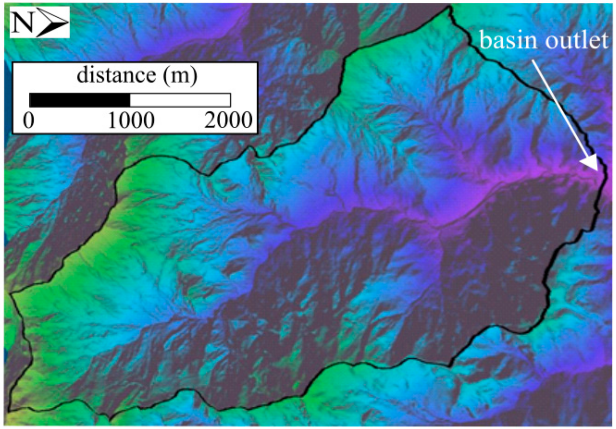
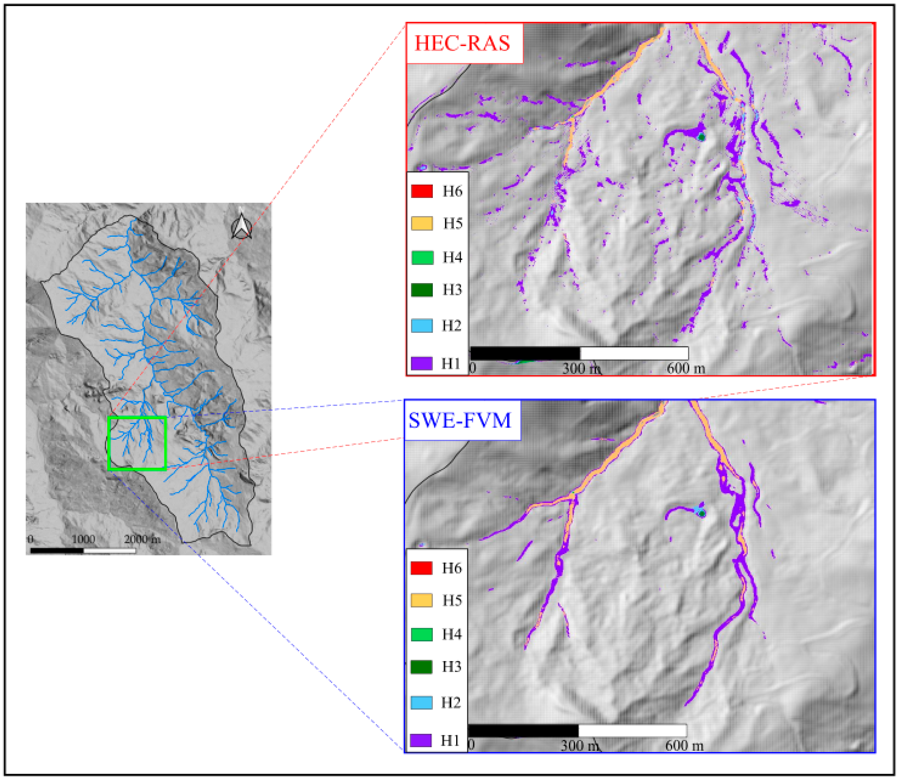
2. Case Study: Scuropasso Basin

The case study analyzed here is a part of the Scuropasso Basin, a tributary of the Po River, flowing in Lombardy Region. Scuropasso is a small basin (43 km2) with an average slope of 12.95%. The sub-catchment area is equal to 13.75 km2 with an elevation at the basin closure section of 187 m a.s.l., a maximum elevation of 537 m a.s.l. and a mean elevation of 187 m above sea level. The sub-catchment mean slope is 24.57%. Agricultural areas represent the dominant land use while urbanization is composed by very small isolated urban agglomeration. A high resolution airborne LiDAR covers the sub-catchment area, providing a sampling density of four points over 1 m2 (see Figure 1).

3. Methods

3.1. Hydrodynamic Models for Surface Runoff

3.1.1. HEC-RAS 5.0.7

HEC-RAS is a complex modelling tool which include a large number of applications for 1D model and recently it solves the fully 2D shallow water equations written as follows:
H t + p x + q y = r
p t + x p 2 h + y p q h = n 2 p g p 2 + q 2 h 2 g h H x + p f + ρ x h τ x x + ρ y h τ x y
q t + x p q h + y q 2 h = n 2 q g p 2 + q 2 h 2 g h H y + q f + ρ x h τ x y + ρ y h τ y y
where H(x,y,t) = z(x,y) + h(x,y,t) is the surface elevation (m), z is the cell elevation in the cartesian coordinates x, y, h is the water depth (m), p = hu and q = hv are the specific flow in the x and y directions (m2 s−1), u and v are the velocities in x and y respectively, r is the net rain (m), g is the gravity acceleration (ms−2), n is the Manning’s roughness coefficient (s m−1/3), ρ is the water density (kg m−3), τxx, τyy and τxy are the components of the stress tensor and f is the Coriolis parameter (s−1). When the diffusive wave is selected, the inertial terms in Equations (2) and (3) are neglected. The above equations are solved with an implicit finite-volume scheme.
HEC-RAS 5.0.7 introduced the capability to compute 2D fully momentum shallow water equation based on unstructured grid joint to a sub-grid based on a high-resolution DEMs, (e.g., LiDAR) which may drastically affect models results as well as performance [33,50]. Hence, the sub-grid approach provides information given by the high resolution DEMs bathymetry. Thus, Equation (1) is presented in the integral form:
Ω H n + 1 Ω H n Δ t + k V k · n k A k H + R = 0
where Ω is the volumetric three-dimensional space occupied by the fluid, R is the source term (net rainfall), Vk is the average velocity at the k face with the normal vector nk, Ak(H) the averaged area at the k face. The superscript n represents the time step and ∆t the integration time. The integral form of Equation (4) is needed to compute extra information (e.g., hydraulic radius, volume, cross-sectional data) in a preprocessing stage for every computational cell face [27,50]. The sub-grid approach can be used to increase the cell dimensions preserving the details of the bathymetry [50].
Finally, in the HEC-RAS 5.0.7 the Courant–Friedrichs–Lewy (CFL) condition is implemented into the model.

3.1.2. Shallow Water Equations-Finite Volume Code

The implemented code (hereinafter called SWE-FVM) for surface runoff simulation is based on the 2-D fully-dynamic SWE that can be expressed in the following form:
U t + F x + G y = S
where:
U = h h u h v ;   F = h u h u 2 + g h 2 / 2 h u v ;   G = h v h u v h v 2 + g h 2 / 2 ;   S = r f g h S 0 x S f x g h S 0 y S f y
in which: t is time; x, y are the horizontal coordinates; h is the water depth; u, v are the depth-averaged flow velocities in x- and y- directions; g is the gravitational acceleration; r is the rain intensity and f are the infiltration losses; S0x, S0y are the bed slopes in x- and y-directions; Sfx, Sfy are the friction slopes in x- and y-directions. For the numerical integration of Equation (5), the finite volume method (FVM) approach has been considered. In particular, the Roe scheme [51], first order accurate in time and space, has been used for the computation of the numerical fluxes. Moreover, suitable numerical treatments of the source terms and wet/dry fronts have been applied [52,53]. The mathematical aspects and performances in real cases have been already presented in previous works [42,54,55] and, therefore, are not reported here. The code is parallelized using MPI directives.

3.2. Computational Grids and Boundary Conditions

The generation of computational grid is one of the key elements for the application of 2-D models because of its influence on the accuracy and on the computational times [56]. Though some methods have been proposed to generate a priori grids, having different resolution throughout the basin [57], the evaluation of the performances of the SWE-FVM and HEC-RAS models will be shown on two different computational grids with uniform resolution. The first one is a fine triangular grid, of 5 m side. This grid represents the most accurate computational domain used in this work (fine grid, hereafter). On the contrary, the second one has an average triangular side of 10 m, being much coarser (coarse grid hereafter). The coarse grid dimension choice is in accordance to literature which assert that a resolution up to 10 m does not influence geomorphologic indices like flow patterns and basin hydrologic responses [58]. The fine grid dimension is based on the availability of the HEC-RAS geometry editor to manage a large number of elements. In order to run properly the two overland flow models, the use of the same grid in both the models is needed. Namely, the computational grid has been created through the external mesh generator SMS 13.0 (Aquaveo—Surface-water Modeling System, https://www.aquaveo.com/software/sms-surface-water-modeling-system-introduction). The SMS software is well-known in the scientific context (see for example [18]). It is not an open source package but is able to export the computational grid in a 0.2 dm format readable in the SWE model as well as in a format compatible with HEC-RAS. This process ensures the uses of the same computational domain by the two models. Finally, the fine grid is composed by 1,293,762 unstructured triangular elements, whereas in the coarse mesh number of elements is 323,161.
Whatever is the grid used by HEC-RAS, the software applied the so-called high-resolution sub-grid model [59], which allows coarse computational meshes to be used without losing the detail of the underlying terrain [50].
As regards the boundary conditions, we have not specified the upstream boundary condition due to the nature of the simulations. Specifically, the approach used here is devoted to generate the surface runoff and, as consequence, the flood wave using only one model (the 2-D SWEs) without using the traditional modelling chain in which the flood hydrograph is computed using a hydrological model and, then, a hydrodynamic model is used for flood propagation. Therefore, there is no need to compute an upstream boundary condition, so the use of the net rainfall on grid avoids the computation of synthetic hydrograph with a given return period. The method used for the computation of the net rainfall is presented in the next section.
As regards the downstream boundary condition, transmissive boundary conditions have been set for the SWE-FVM model while the “normal depth” option has been selected for the HEC-RAS model, that means uniform flow condition.

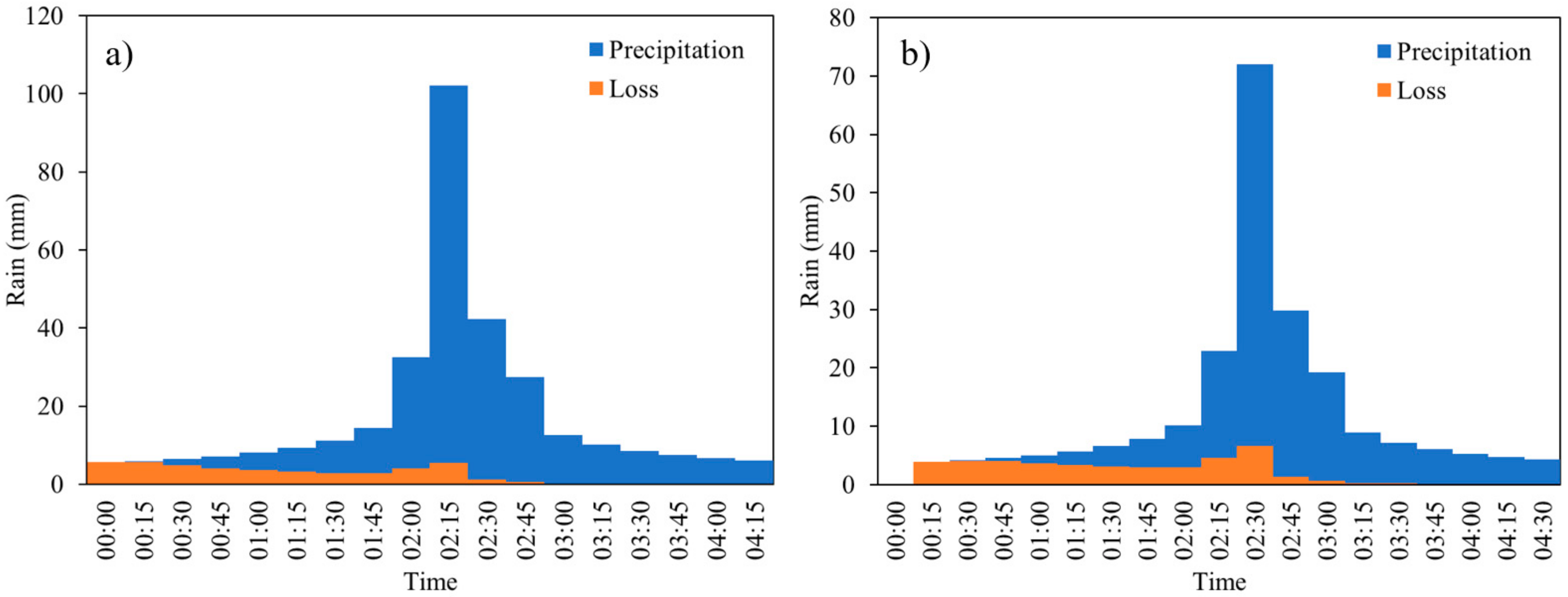
3.3. Net Rainfall Computation and Roughness Estimation

The intent of the comparative analysis shown in this work is to analyze the discrepancy between the models results in cases for which no observed data, related to rainfall, flooded areas and discharge, are available. This is the typical situation in small basins that, very often, are ungauged catchments for which is not possible to have data for model calibration and validation. As a consequence, “blind” simulations should be performed. In our view, in situations like these, is important to assess the performance of a commercial software using a state-of-the art model, developed for research purposes, as the benchmark solution. For these reasons, we have not considered an observed event for model comparisons. Instead, following a technical approach, two rainfall events were considered to compare the two models, having a return period of T1 = 30 and T2 = 200 years respectively. The Chicago hyetograph was adopted using the rainfall intensity-duration curve taken from the Regional Agency for the Protection of the Environment (ARPA) website, which is evaluated taking into accounts data from 1987 to 2011 (http://idro.arpalombardia.it). The intensity-duration curve used is the following:
h = 24.53 t0.307
The net rainfall was evaluated with the well-known SCS-CN method [60], considering an average Curve Number of 86 for the sub-basin and adopting the initial loss as the 20% of the maximum infiltration losses. The basin Runoff Curve Number was determined for soil in average moisture conditions. Figure 2 shows the net hyetographs for the two adopted return periods.
Therefore, a total of 4 simulations were performed for each model, considering rainfall events having 30 years and 200 years of return period and for the two grids described in the previous section.
As regards the Manning’s roughness coefficients, we set the following values according to the available map related to the use of soil: 0.035 s m−1/3, 0.06 s m−1/3 and 0.1 s m−1/3 for agricultural areas forest and urbanized areas respectively.

3.4. Flood Hazard Estimation

Several methods are available in the literature for flood hazard estimation. In this work, we refer to the method proposed by [61], recommended by [62] and recently analyzed in [13,63,64,65]. This criterion, also known as Australian Institute for Disaster Resilience (AIDR) hazard classification, combines information related to water depth h and velocity V, defining six hazard classes. We have selected this criterion essentially due to its simplicity and because it considers the main targets exposed to flood risk (see Table 1).

3.5. Performance Measures

The overlapping of the flooded areas belonging to the different AIDR classes can be performed through several indexes, widely used in the literature. Specifically, in this work we use the Hit Rate, False Alarm Ratio, Critical Success Index [66].
The Hit Rate (HR), sometimes referred to as the probability of detection, is a simple measure that indicates how well the model replicates the benchmark data without penalizing for overprediction. It is defined as:
HR = A x A R A R
and it is equal to 0 when all wet areas of the two models are totally separated whereas is 1 when all wet cells in the benchmark data are wet in the model x, being Ax the modeled inundated area and AR is the benchmark inundated area.
The False Alarm Ratio (FAR) is a measure of model overprediction. It is defined as:
FAR = A x \ A R A x A R + A x \ A R
The values of FAR ranges between 0, when no false alarms are present, and 1 when there are all false alarms.
The Critical Success Index (CSI) is defined as:
CSI = A x A R A x A R
CSI = 0 means no match between model x and the benchmark, CSI = 1 implies perfect match. Finally, a simple measure of error bias B can be defined as:
B = A x \ A R A R \ A x
When B ranges between 0 and 1, the model x shows a tendency to underpredict the benchmark, whereas B between 1 and ∞ indicated the tendency of the model to overpredict.

4. Results and Discussion

The comparison between the performances of HEC-RAS and the SWE model is presented here. Attention will be first focused on the simulated discharges hydrographs at the basin outlet, then will be oriented to the flooded areas mapping and finally to the flood hazard assessment according to the predictions of the two models.

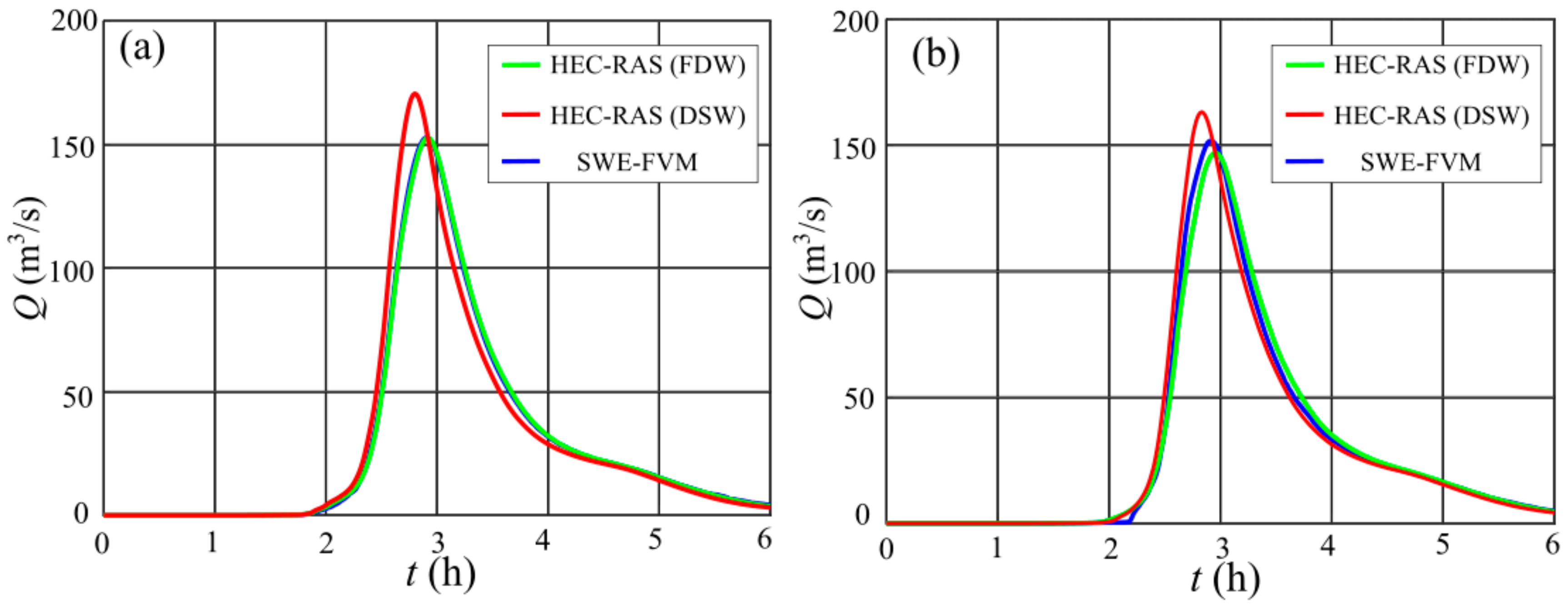
4.1. Discharge Hydrographs at the Basin Outlet

HEC-RAS has been used according the two options: full momentum and the diffusion wave approximation, hereafter identified as FDW (Fully Dynamic Wave) and DSW (DiffuSive Wave) respectively. Figure 3 and Figure 4 show the comparison of the discharge hydrographs at the basin outlet simulated by the two models for a return period of 200 years and 30 years respectively, using two different grid resolutions. The FDW version of HEC-RAS gives very similar results in terms of the flood wave shape, peak discharge and time to peak in respect of SWE-FVM (see Table 2). In particular, for the smaller grid resolution, HEC-RAS results are practically superimposed to those ones obtained by SWE-FVM model (see Figure 3a and Figure 4a). However, it is interesting to stress that the grid resolution has a very small influence in terms of flood hydrographs. Specifically, the SWE-FVM model results are quite insensitive to the analyzed grid resolution while, considering HEC-RAS, the peak discharge for the 10-m resolution is slightly lower (approximately 4%) than the homologous one related to the 5-m resolution (Figure 3b and Figure 4b). This behavior can be observed for both the analyzed return periods. The flood hydrographs simulated by the DSW version of HEC-RAS are slightly different from the other two simulated waves.
In particular, the peak discharges values are overestimated (about 12%) if compared to the other two simulations for both the return periods. The DSW model shows a tendency to simulate faster flood waves (see Table 2). These differences seem to decrease with the increase of the grid size. The sensitivity of the DSW to the grid resolution might be explained considering that, in this approach, the velocity is depending almost entirely on the slope of the terrain.
Finally, it is interesting to discuss the HEC-RAS performance in terms of overall computational times. HEC-RAS simulations were computed on a AMD Ryzen 2700X processor Eight-Core Processor 3.70 GHz (AMD, Santa Clara, CA, United States), with 32 GB RAM.
Table 2 shows that the simulations carried out using the finest grid resolution are not particularly feasible for practical study, resulting more than four times greater the duration of the real flood event. The reduction of the computational times obtained using the DSW option is not significant (about 5–6%). Conversely, the performances related to the coarsest grid are interesting. The FDW option has provided results in a shorter time respect to real event duration (see Table 2) for both the return periods, while the DSW option allowed a further decrease of the runtimes in respect of the FDW ones (about 40%). Obviously, these performances cannot be compared to the SWE-FVM, because the latter model has been parallelized using MPI directives and computed on a cluster using 192 threads. This justifies the very good performances of the SWE-FVM, which is faster than HEC-RAS (about one-order of magnitude).
The analysis that follows will be focused only on the comparison between the FDW option of HEC-RAS and SWE-FVM, due to the very similar performances of the two models in terms of simulated discharge hydrographs.

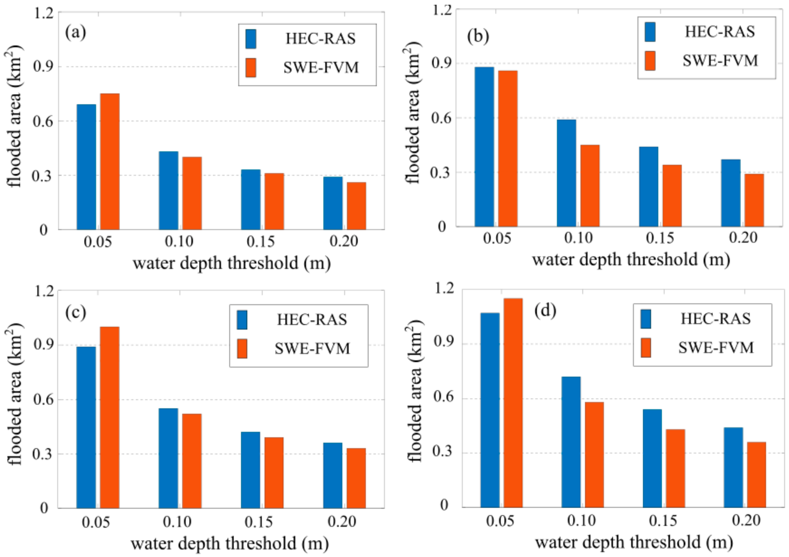
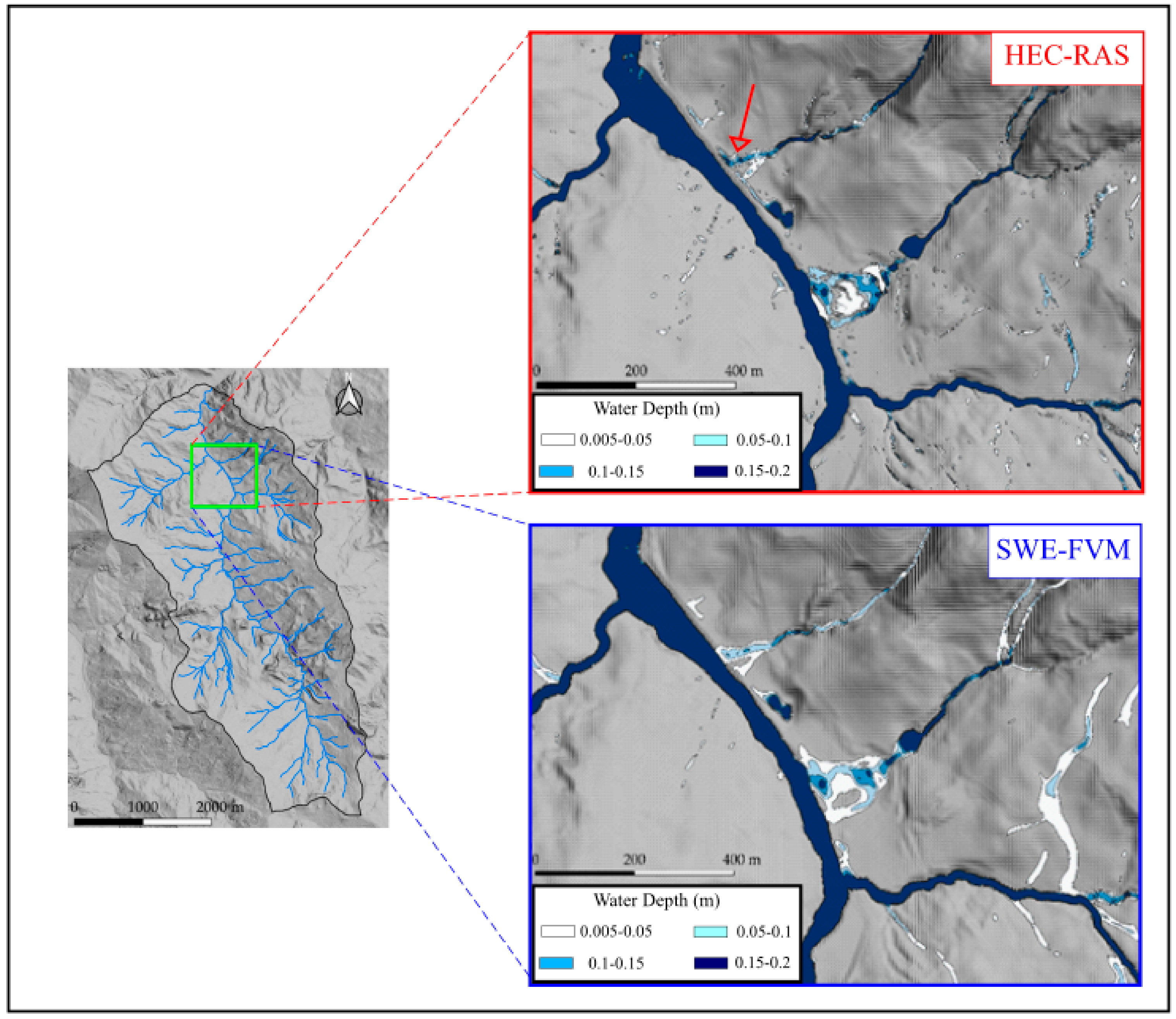
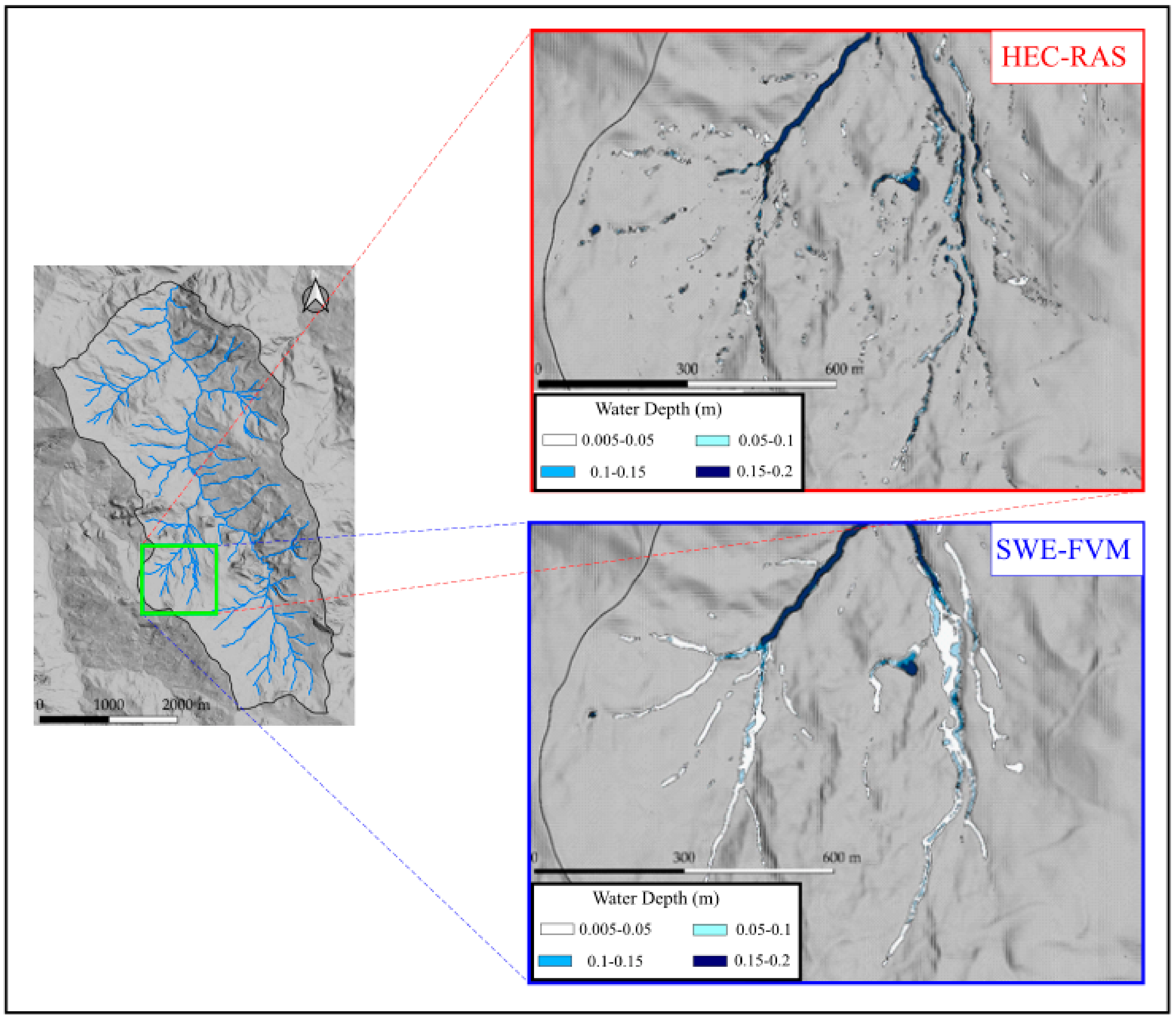
4.2. Simulated Flooded Area Extent

Beside the discharge hydrograph at the outlet, one of most important information for flood hazard assessment is the flooded areas delimitation. For rainfall-runoff simulations at the basin scale, since the rainfall input is applied to each computational cell, it is necessary to define a water depth threshold for the identification of the flooded cells.
Though some methods have been proposed in the literature (see [42]), in this work we have analyzed the flooded areas for different, very small water levels. Table 3 shows the extent of the flooded areas, computed by the two models, equal to or greater than pre-fixed water depth thresholds (5, 10, 15 and 20 cm).
In Figure 5, the comparison between the flooded areas computed by the two models for each return period and grid size is shown. For the fine grid, the overall results seem to be comparable while, for the coarse one, some significant differences appear. Figure 6 shows the relative variations in the flooded area, computed by Equation (12), taking SWE-FVM results as reference solution, for both the different grid resolutions and the return periods:
Relative   Variation   h = A H R h A S F h / A S F h
where AHR(h) and ASF(h) represent the flooded area related to the threshold h as simulated by HEC-RAS and SWE-FVM respectively.
Greater variations are found for the bigger cell dimension. Neglecting the first threshold value, HEC-RAS always overestimates SWE-FVM flooded areas with variations approximately equal to 5–10% and 20–30% for the fine grid and coarse grid, respectively. For some water depth thresholds, the variation due to the 10-m resolution grid is up to three times the one computed for the 5-m resolution grid (see Figure 6a). The decrease in the difference between model results, as the grid size increases, might be explained considering that, at lower resolutions, the small-scale characteristics, which may be handled differently in the models, become negligible and thus the results converge.
If a more severe event is considered (Tr 200 year vs. 30 year), the variations between the two models generally decrease for the coarse grid while are substantially constant for the fine one (Figure 6b). Therefore, the variations in flooded areas increase as the cell size increases and as the return period decreases, at least for the coarse grid.
The smaller water depth threshold is the only value for which HEC-RAS provided an underestimation of the flooded area. In order to better understand what happens in this situation, the extent of the flooded area computed by the two models in two particular zones of the sub-basin, one upstream and one close to the closure section, have been analyzed. Figure 7 and Figure 8 show the flood extent related to a return period of 200 years, using the fine grid resolution. In those figures, the river network simulated by HEC-RAS is characterized by quite disconnected flooded areas. Looking at the Figure 7, it is clear that the tributary highlighted by the red arrow does not flow into the main channel or, in other words, the tributary is not connected to the main channel. Moreover, the part of the network having smaller Horton orders is quite fragmented and, in general, underestimated. This is enhanced in Figure 8 where the network described by HEC RAS gets to a cloud of small areas disconnected one from the other.
This observation can be considered a generalization of what has been already noted by [33], who observed, in a traditional flood propagation study, a certain amount of hydraulically disconnected flooded areas, that is areas simulated as flooded but disconnected from the main inundated area. This could be induced by the way in which HEC-RAS distributes the water within a computational cell, based also on the volume-elevation curve drawn for each cell-face in pre-processing stage. However, the current study did not look into the specific features of this property.

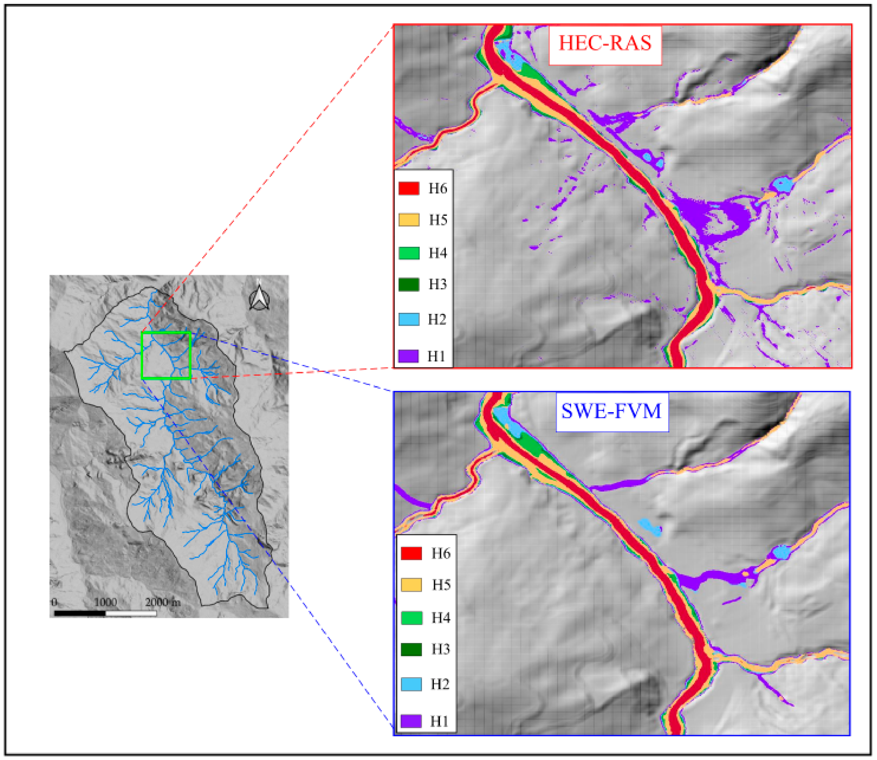
4.3. Flood Hazard Classification

The water depths and velocity fields simulated by the two models have been used for flood hazard mapping purposes. As mentioned in Section 3.4, the criterion proposed in [62] have been considered here according to which six hazard classes can be identified as a function of h and V. The results obtained using this approach are reported in Figure 9 for each return period and grid resolution, showing the distribution of the flooded areas belonging to each class.
Looking at the H2, H3 and H4 classes, the flooded areas simulated by HEC-RAS are generally comparable to those computed by SWE-FVM. However, the flooded area falling in class H1 is significantly overestimated. The latter discrepancy may be ascribed to the way HEC-RAS redistributes the water depth in the computational cell, defined as the sub-grid approach. Moreover the two models give different flooded area for smaller water depths. These variations seem to decrease with the return period (Figure 9a,b, or Figure 9c,d) and to increase with the cell size (Figure 9a,c, or Figure 9b,d). Another significant difference between the two models can be found in the class H5, in which the HEC-RAS results underestimate the results obtained by SWE-FVM model. This variation seems to increase as the return period decreases (Figure 9a,b, or Figure 9c,d).
Figure 9 gives an overall description of the flooded areas extent simulated by the two models but it cannot provide any information about their overlapping from a topographic point of view. To that purpose, it is necessary to use performance indexes mentioned in Section 3.4. For the sake of brevity, only the finer grid results (cell size equal to 5 m) are reported in Table 4 and Table 5, related to the return period 30 years and 200 years, respectively.
The values of the CSI index highlight that the areas flooded by the two models are far to be coincident, at least for the first five classes. This is further confirmed by the HR values that show a value close to 1 only for the H6 class. The values assumed by B seem to suggest the HEC-RAS simulation underestimate the flooded area belonging to the classes H4 and H5 while it is overestimated especially in the first three classes
Generally, these measures seem not to be significantly affected by the flood magnitude and therefore by the return periods considered here.
Figure 10 and Figure 11 show the comparison between the hazard maps computed by the two models in the two selected areas discussed in Figure 7 and Figure 8. While in the river network the hazard classes computed by the two models seem to be close together, it is interesting to note that HEC-RAS defines zones far from the network in H1 and H2 classes. In these areas, water depths are smaller than the selected threshold (0.05 m), meaning that very high velocities are found.

5. Conclusions

This work has been focused on the performance of the new HEC-RAS 5.0.7 for the hydrodynamic-based surface runoff computations in rainfall-runoff simulations at the catchment scale. Contrarily to the common applications for flood propagation in river reach, this work shows for the first time a critical discussion of this specific new module, never analyzed in the literature.
Specifically, in order to assess its potential and the capabilities, HEC-RAS has been applied to a small basin in Italy and compared to the results obtained by a 2-D fully dynamic model developed by the authors (SWE-FVM). The main conclusions of this paper are listed below:
  • Using the “full momentum” options, HEC-RAS has provided very similar results in terms of the flood wave shape, peak discharge and time to peak in respect of SWE-FVM. The diffusive wave version (DSW) of HEC-RAS overestimates the peak discharges values computed by the other two models, showing a tendency to simulate faster flood waves;
  • The reduction of the computational times obtained using the DSW option is not significant for finer grid but it becomes important using a coarser one, with time savings up to 40%;
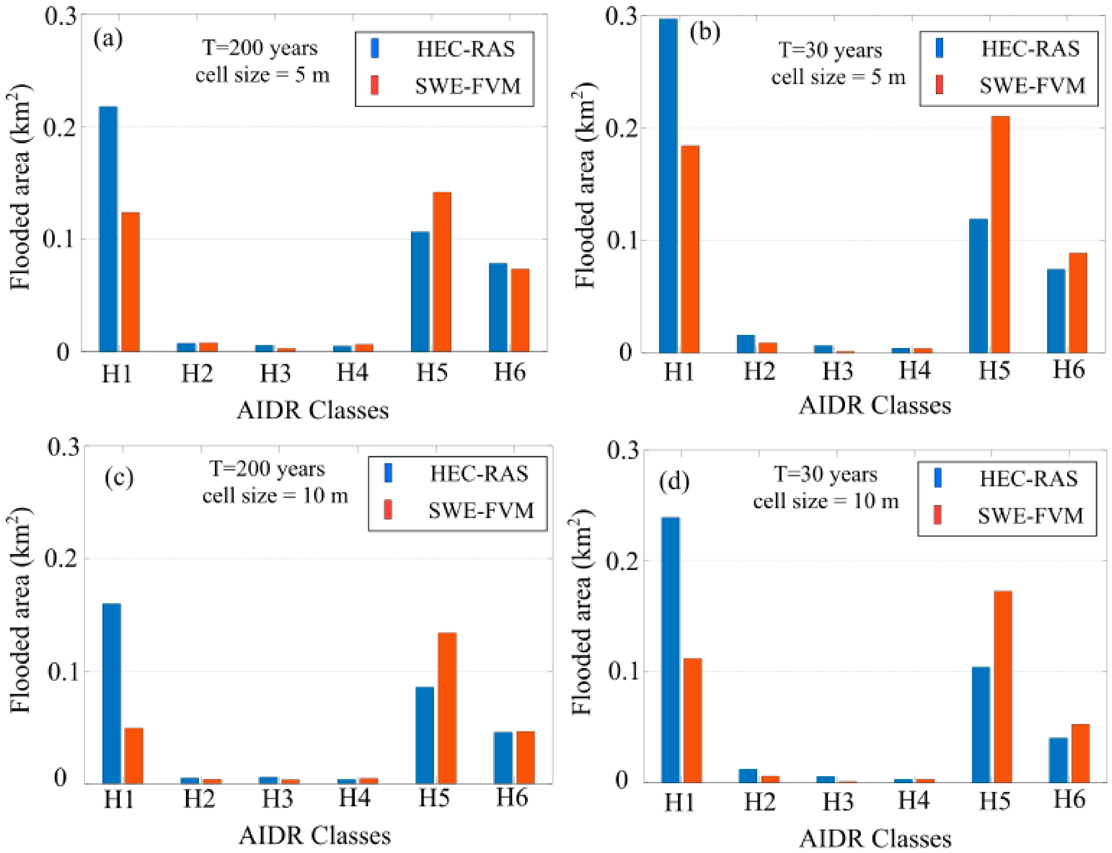
  • The analysis of flood extent, carried out for different pre-fixed water depth thresholds, highlights that, except for the smaller threshold, HEC-RAS has always overestimated the SWE-FVM flooded areas with variations approximately equal to 5–10% and 20–30% for the fine grid and coarse grid respectively. The variations in terms of flooded areas increase as the cell size increases and the return period decreases, at least for the coarse grid;
  • The flooded area related to the first threshold (0.05 m) is underestimated in respect to the SWE-FVM one. In particular, the part of the network having lower Horton-Strahler order is described by HEC-RAS as disconnected, while HEC-RAS and the SWE-FVM models describe the main channel in a similar way;
  • The application of the AIDR criterion for hazard class mapping has highlighted significant variations between the two models. For example, in respect to the SWE-FDW results, HEC-RAS has significantly underestimated the flooded areas related to the H5 class while an important overestimation has been observed for the H1 class;
  • The application of the performance measures has highlighted that the areas flooded by the two models belonging to a specific hazard class are far to be coincident, at least for the first five classes.
These results highlight the need of further investigations and a larger number of case studies in order to generalize these conclusions. However, on the basis of this first study, it seems that HEC-RAS can be considered as a reliable model for discharge hydrograph computation in rainfall-runoff simulations.

Author Contributions

Conceptualization, P.C. and C.C.; Data curation, D.F. and G.P.; Investigation, C.C., F.M. and G.P.; Methodology, P.C.; Project administration, G.P.; Software, C.C. and D.F.; Supervision, F.M.; Visualization, D.F.; Writing—original draft, P.C.; Writing—review & editing, P.C. and F.M. All authors have read and agreed to the published version of the manuscript.

Funding

This work has been in the frame of the ANDROMEDA project, which has been supported by Fondazione Cariplo, grant n 2017-067. For the co-authors belonging to University of Calabria, this work was supported in part by the funding project PON SILA-PONa3_00341A (LaMPIT Laboratory, Scient. Head: F. Macchione).

Conflicts of Interest

The authors declare no conflict of interest.

References

  1. EXCIMAP. Handbook on Good Practices for Flood Mapping in Europe. European Exchange of Circle on Flood Mapping. Available online: https://ec.europa.eu/environment/water/flood_risk/flood_atlas/pdf/handbook_goodpractice.pdf (accessed on 17 August 2020).
  2. Petaccia, G.; Natale, E. Orsadem: A one-dimensional shallow water code for flood inundation modelling. Irrig. Drain. 2013, 62, 29–40. [Google Scholar] [CrossRef]
  3. Costabile, P.; Macchione, F. Analysis of One-Dimensional Modelling for Flood Routing in Compound Channels. Water Resour. Manag. 2012, 26, 1065–1087. [Google Scholar]
  4. Horritt, M.S.; Bates, P.D. Evaluation of 1D and 2D numerical models for predicting river flood inundation. J. Hydrol. 2002, 268, 87–99. [Google Scholar]
  5. Tayefi, V.; Lane, S.N.; Hardy, R.J.; Yu, D. A comparison of one- and two-dimensional approaches to modelling flood inundation over complex upland floodplains. Hydrol. Process. 2007, 21, 3190–3202. [Google Scholar]
  6. Falter, D.; Vorogushyn, S.; Lhomme, J.; Apel, H.; Gouldby, B.; Merz, B. Hydraulic model evaluation for large-scale flood risk assessments. Hydrol. Process. 2013, 27, 1331–1340. [Google Scholar]
  7. Costabile, P.; Macchione, F.; Natale, L.; Petaccia, G. Flood mapping using LIDAR DEM. Limitations of the 1-D modeling highlighted by the 2-D approach. Nat. Hazards 2015, 77, 181–204. [Google Scholar]
  8. Costabile, P.; Macchione, F.; Natale, L.; Petaccia, G. Comparison of scenarios with and without bridges and analysis of backwater effect in 1-D and 2-D river flood modeling. CMES Comp. Model. Eng. Sci. 2015, 109, 81–103. [Google Scholar]
  9. Martínez-Gomariz, E.; Gómez, M.; Russo, B.; Djordjević, S. Stability criteria for flooded vehicles: A state-of-the-art review. J. Flood Risk Manag. 2018, 11, S817–S826. [Google Scholar]
  10. Bermúdez, M.; Zischg, A.P. Sensitivity of flood loss estimates to building representation and flow depth attribution methods in micro-scale flood modelling. Nat. Hazards 2018, 92, 1633–1648. [Google Scholar]
  11. Arrighi, C.; Pregnolato, M.; Dawson, R.J.; Castelli, F. Preparedness against mobility disruption by floods. Sci. Total Environ. 2019, 654, 1010–1022. [Google Scholar] [CrossRef]
  12. Macchione, F.; Costabile, P.; Costanzo, C.; Gangi, F. Modello idraulico per l’analisi a scala di bacino della pericolosità delle piene impulsive. In Fully-Hydrodynamics Watershed Model for Flash-Flood Hazard Analysis, Proceedings of the Italian Conference on Integrated River Basin Management (ICIRBM—Guardia 2019), Guardia Piemontese, CS, Italy, 19–22 June 2019; EdiBios: Cosenza, Italy, 2019; Volume 40, pp. 105–117. ISSN 2282–5517. [Google Scholar]
  13. Costabile, P.; Costanzo, C.; De Lorenzo, G.; Macchione, F. Is local flood hazard assessment in urban areas significantly influenced by the physical complexity of the hydrodynamic inundation model? J. Hydrol. 2020, 580, 124231. [Google Scholar] [CrossRef]
  14. Petaccia, G.; Natale, L. 1935 Sella Zerbino dam break case revisited: A new hydrologic and hydraulic analysis. J. Hydraul. Eng. 2020, 146. [Google Scholar] [CrossRef]
  15. Mignot, E.; Paquier, A.; Haider, S. Modeling floods in a dense urban area using 2D shallow water equations. J. Hydrol. 2006, 327, 186–199. [Google Scholar] [CrossRef] [Green Version]
  16. Brath, A.; Carisi, F.; Domeneghetti, A.; Castellarin, A. Modelli di danno da alluvione uni- e multi-variati: Esperienze acquisite dall’evento alluvionale del fume Secchia. In Uni- and Multi-Variable Modelling of Flood Losses: Experiences Gained from the Secchia River Inundation Event, Proceedings of the Italian Conference on Integrated River Basin Management (ICIRBM—Guardia 2019), Guardia Piemontese, CS, Italy, 19–22 June 2019; EdiBios: Cosenza, Italy, 2019; Volume 40, pp. 15–27. ISSN 2282-5517. [Google Scholar]
  17. Ernst, J.; Dewals, B.J.; Detrembleur, S.; Archambeau, P.; Erpicum, S.; Pirotton, M. Micro-scale flood risk analysis based on detailed 2D hydraulic modelling and high resolution geographic data. Nat. Hazards 2010, 55, 181–209. [Google Scholar]
  18. Costabile, P.; Macchione, F. Enhancing river model set-up for 2-D dynamic flood modelling. Environ. Model. Softw. 2015, 67, 89–107. [Google Scholar] [CrossRef]
  19. Dazzi, S.; Vacondio, R.; Mignosa, P. Integration of a Levee Breach Erosion Model in a GPU-Accelerated 2D Shallow Water Equations Code. Water Resour. Res. 2019, 55, 682–702. [Google Scholar] [CrossRef]
  20. Lacasta, A.; Morales-Hernández, M.; Murillo, J.; García-Navarro, P. GPU implementation of the 2D shallow water equations for the simulation of rainfall/runoff events. Environ. Earth Sci. 2015, 74, 7295–7305. [Google Scholar] [CrossRef]
  21. Vacondio, R.; Dal Palù, A.; Ferrari, A.; Mignosa, P.; Aureli, F.; Dazzi, S. A non-uniform efficient grid type for GPU-parallel Shallow Water Equations models. Environ. Model. Softw. 2017, 88, 119–137. [Google Scholar]
  22. Hu, P.; Lei, Y.; Han, J.; Cao, Z.; Liu, H.; He, Z. Computationally efficient modeling of hydro-sediment-morphodynamic processes using a hybrid local time step/global maximum time step. Adv. Water Resour. 2019, 127, 26–38. [Google Scholar] [CrossRef]
  23. Simões, N.E.; Ochoa-Rodríguez, S.; Wang, L.-P.; Pina, R.D.; Marques, A.S.; Onof, C.; Leitão, J.P. Stochastic urban pluvial flood hazard maps based upon a spatial-temporal rainfall generator. Water 2015, 7, 3396–3406. [Google Scholar] [CrossRef]
  24. Liu, Z.; Merwade, V.; Jafarzadegan, K. Investigating the role of model structure and surface roughness in generating flood inundation extents using one- and two-dimensional hydraulic models. J. Flood Risk Manag. 2019, 12, e12347. [Google Scholar] [CrossRef] [Green Version]
  25. Sole, A.; Albano, R.; Samela, C.; Craciun, I.; Perrone, A.; Manfreda, S.; Ozunu, A. Mappatura del danno alluvionale a vasta scala: Un’applicazione in Romania. In Large Scale Flood Risk Mapping: An Application over Romania, Proceedings of the Italian Conference on Integrated River Basin Management (ICIRBM—Guardia 2019), Guardia Piemontese, CS, Italy, 19–22 June 2019; EdiBios: Cosenza, Italy, 2019; Volume 40, pp. 77–90. ISSN 2282-5517. [Google Scholar]
  26. Bomers, A.; Schielen, R.M.J.; Hulscher, S.J.M.H. Application of a lower-fidelity surrogate hydraulic model for historic flood reconstruction. Environ. Model. Softw. 2019, 117, 223–236. [Google Scholar] [CrossRef] [Green Version]
  27. Quirogaa, V.M.; Kurea, S.; Udoa, K.; Manoa, A. Application of 2D numerical simulation for the analysis of the February 2014 Bolivian Amazonia flood: Application of the new HEC-RAS version 5. RIBAGUA 2016, 3, 25–33. [Google Scholar] [CrossRef] [Green Version]
  28. Lea, D.; Yeonsu, K.; Hyunuk, A. Case study of HEC-RAS 1D-2D coupling simulation: 2002 Baeksan flood event in Korea. Water 2019, 11, 2048. [Google Scholar] [CrossRef] [Green Version]
  29. Patel, D.P.; Ramirez, J.A.; Srivastava, P.K.; Bray, M.; Han, D. Assessment of flood inundation mapping of Surat city by coupled 1D/2D hydrodynamic modeling: A case application of the new HEC-RAS 5. Nat. Hazards 2017, 89, 93–130. [Google Scholar] [CrossRef]
  30. Pasquier, U.; He, Y.; Hooton, S.; Goulden, M.; Hiscock, K.M. An integrated 1D–2D hydraulic modelling approach to assess the sensitivity of a coastal region to compound flooding hazard under climate change. Nat. Hazards 2019, 98, 915–937. [Google Scholar]
  31. Pinos, J.; Timbe, L. Performance assessment of two-dimensional hydraulic models for generation of flood inundation maps in mountain river basins. Water Sci. Eng. 2019, 12, 11–18. [Google Scholar] [CrossRef]
  32. Vozinaki, A.-E.K.; Morianou, G.G.; Alexakis, D.D.; Tsanis, I.K. Comparing 1D and combined 1D/2D hydraulic simulations using high-resolution topographic data: A case study of the Koiliaris basin, Greece. Hydrol. Sci. J. 2017, 62, 642–656. [Google Scholar]
  33. Shustikova, I.; Domeneghetti, A.; Neal, J.C.; Bates, P.; Castellarin, A. Comparing 2D capabilities of HEC-RAS and LISFLOOD-FP on complex topography. Hydrol. Sci. J. 2019, 64, 1769–1782. [Google Scholar] [CrossRef]
  34. Pilotti, M.; Milanesi, L.; Bacchi, V.; Tomirotti, M.; Maranzoni, A. Dam-Break Wave Propagation in Alpine Valley with HEC-RAS 2D: Experimental Cancano Test Case. J. Hydraul. Eng. 2020, 146, 05020003. [Google Scholar]
  35. Afshari, S.; Tavakoly, A.A.; Rajib, M.A.; Zheng, X.; Follum, M.L.; Omranian, E.; Fekete, B.M. Comparison of new generation low-complexity flood inundation mapping tools with a hydrodynamic model. J. Hydrol. 2018, 556, 539–556. [Google Scholar]
  36. Jamali, B.; Bach, P.M.; Cunningham, L.; Deletic, A. A Cellular Automata Fast Flood Evaluation (CA-ffé) Model. Water Resour. Res. 2019, 55, 4936–4953. [Google Scholar] [CrossRef] [Green Version]
  37. Yalcin, E. Assessing the impact of topography and land cover data resolutions on two-dimensional HEC-RAS hydrodynamic model simulations for urban flood hazard analysis. Nat. Hazards 2020, 101, 995–1017. [Google Scholar] [CrossRef]
  38. Mihu-Pintilie, A.; Cîmpianu, C.I.; Stoleriu, C.C.; Pérez, M.N.; Paveluc, L.E. Using high-density LiDAR data and 2D streamflow hydraulic modeling to improve urban flood hazard maps: A HEC-RAS multi-scenario approach. Water 2019, 11, 1832. [Google Scholar] [CrossRef] [Green Version]
  39. Stoleriu, C.C.; Urzica, A.; Mihu-Pintilie, A. Improving flood risk map accuracy using high-density LiDAR data and the HEC-RAS river analysis system: A case study from north-eastern Romania. J. Flood Risk Manag. 2019, 13, e12572. [Google Scholar] [CrossRef]
  40. Yu, F.; Harbor, J.M. The effects of topographic depressions on multiscale overland flow connectivity: A high-resolution spatiotemporal pattern analysis approach based on connectivity statistics. Hydrol. Process. 2019, 33, 1403–1419. [Google Scholar] [CrossRef]
  41. Hall, J. Direct rainfall flood modelling: The good, the bad and the ugly. Australas. J. Water Resour. 2015, 19, 74–85. [Google Scholar] [CrossRef]
  42. Costabile, P.; Costanzo, C.; De Bartolo, S.; Gangi, F.; Macchione, F.; Tomasicchio, G.R. Hydraulic Characterization of River Networks Based on Flow Patterns Simulated by 2-D Shallow Water Modeling: Scaling Properties, Multifractal Interpretation, and Perspectives for Channel Heads Detection. Water Resour. Res. 2019, 55, 7717–7752. [Google Scholar]
  43. Cea, L.; Garrido, M.; Puertas, J. Experimental validation of two-dimensional depth-averaged models for forecasting rainfall-runoff from precipitation data in urban areas. J. Hydrol. 2010, 382, 88–102. [Google Scholar] [CrossRef]
  44. Fernández-Pato, J.; Caviedes-Voullième, D.; García-Navarro, P. Rainfall/runoff simulation with 2D full shallow water equations: Sensitivity analysis and calibration of infiltration parameters. J. Hydrol. 2016, 536, 496–513. [Google Scholar]
  45. Bout, B.; Jetten, V.G. The validity of flow approximations when simulating catchment-integrated flash floods. J. Hydrol. 2018, 556, 674–688. [Google Scholar]
  46. Xia, X.; Liang, Q.; Ming, X. A full-scale fluvial flood modelling framework based on a high-performance integrated hydrodynamic modelling system (HiPIMS). Adv. Water Resour. 2019, 132, 103392. [Google Scholar]
  47. Caviedes-Voullième, D.; Fernández-Pato, J.; Hinz, C. Performance assessment of 2D Zero-Inertia and Shallow Water models for simulating rainfall-runoff processes. J. Hydrol. 2020, 584, 124663. [Google Scholar]
  48. Bellos, V.; Papageorgaki, I.; Kourtis, I.; Vangelis, H.; Kalogiros, I.; Tsakiris, G. Reconstruction of a flash flood event using a 2D hydrodynamic model under spatial and temporal variability of storm. Nat. Hazards 2020, 101, 711–726. [Google Scholar] [CrossRef]
  49. Aureli, F.; Prost, F.; Vacondio, R.; Dazzi, S.; Ferrari, A. A GPU-accelerated shallow-water scheme for surface runoff simulations. Water 2020, 12, 637. [Google Scholar]
  50. Brunner, G.W. HEC-RAS River Analysis System. HYDRAULIC Reference Manual. Version 5.0; Hydrologic Engineering Center: Davis, CA, USA, 2016.
  51. Roe, P.L. Approximate Riemann solvers, parameter vectors, and difference schemes. J. Comput. Phys. 1981, 43, 357–372. [Google Scholar]
  52. Costabile, P.; Costanzo, C.; Macchione, F. A storm event watershed model for surface runoff based on 2D fully dynamic wave equations. Hydrol. Process. 2013, 27, 554–569. [Google Scholar]
  53. Cea, L.; Bladé, E. A simple and efficient unstructured finite volume scheme for solving the shallow water equations in overland flow applications. Water Resour. Res. 2015, 51, 5464–5486. [Google Scholar]
  54. Costabile, P.; Costanzo, C.; Macchione, F. Two-dimensional numerical models for overland flow simulations. WIT Trans. Ecol. Environ. 2012, 124, 137–148. [Google Scholar]
  55. Macchione, F.; Costabile, P.; Costanzo, C.; De Lorenzo, G. Extracting quantitative data from non-conventional information for the hydraulic reconstruction of past urban flood events. A case study. J. Hydrol. 2019, 576, 443–465. [Google Scholar]
  56. Kim, B.; Sanders, B.F.; Schubert, J.E.; Famiglietti, J.S. Mesh type tradeoffs in 2D hydrodynamic modeling of flooding with a Godunov-based flow solver. Adv. Water Resour 2014, 68, 42–61. [Google Scholar] [CrossRef] [Green Version]
  57. Ferraro, D.; Costabile, P.; Costanzo, C.; Petaccia, G.; Macchione, F. A spectral analysis approach for the a priori generation of computational grids in the 2-D hydrodynamic-based runoff simulations at a basin scale. J. Hydrol. 2020, 582, 124508. [Google Scholar] [CrossRef]
  58. Zhang, W.; Montgomery, D.R. Digital elevation model grid size, landscape representation, and hydrologic simulations. Water Resour. Res. 1994, 30, 1019–1028. [Google Scholar] [CrossRef]
  59. Casulli, V.; Stelling, G.S. Semi-implicit subgrid modelling of three-dimensional free-surface flows. Int. J. Numer. Methods Fluids 2011, 67, 441–449. [Google Scholar] [CrossRef]
  60. United States Soil Conservation Service (S.C.S.). National Engineering Handbook, Section 4—Hydrology; Dept. of Agriculture, Soil Conservation Service: Washington, DC, USA, 1985.
  61. Smith, G.P.; Davey, E.K.; Cox, R.J. Flood Hazard. Technical Report 2014/07; Water Research Laboratory, University of New South Wales: Sydney, Australia, 2014. [Google Scholar]
  62. AIDR. Flood Hazard. Australian Disaster Resilience Handbook Collection. Guide 7–3. 2017. Available online: https://knowledge.aidr.org.au/media/3518/adr-guideline-7-3.pdf (accessed on 17 August 2020).
  63. Bocanegra, R.A.; Vallés-Morán, F.J.; Francés, F. Review and analysis of vehicles stability models during floods and proposal for future improvements. J. Flood Risk Manag. 2019, 13, e12551. [Google Scholar] [CrossRef] [Green Version]
  64. Gangi, F. Applicazione delle Shallow Water Equations per la Simulazione Numerica a Scala di Bacino Degli Eventi Alluvionali. Ph.D. Thesis, University of Calabria, Rende, Italy, 2020. [Google Scholar]
  65. Macchione, F.; Gangi, F.; Costanzo, C.; Costabile, P.; Lombardo, M. Influenza della risoluzione spaziale dei domini di calcolo sull’analisi della pericolosità idraulica a scala di bacino. In Grid Resolution Effects on the Flood Hazard Assessment at the Basin Scale, Proceedings of the Italian Conference on Integrated River Basin Management (ICIRBM—Guardia 2020), Guardia Piemontese, CS, Italy, 17–20 June 2020; EdiBios: Cosenza, Italy, 2020; Volume 41, pp. 41–54. ISSN 2282–5517. [Google Scholar]
  66. Sampson, C.C.; Smith, A.M.; Bates, P.B.; Neal, J.C.; Alfieri, L.; Freer, J.E. A high-resolution global flood hazard model. Water Resour. Res. 2015, 51, 7358–7381. [Google Scholar]
Figure 1. Scuropasso catchment.
Water 12 02326 g001
Figure 2. Net hyetographs for 30 years (a) and 200 years (b), respectively.
Water 12 02326 g002
Figure 3. Discharge hydrograph simulated with HEC-RAS and SWE-FVM models for a return period of 200 years: element size 5 m (a) and 10 m (b).
Water 12 02326 g003
Figure 4. Discharge hydrograph simulated with HEC-RAS and SWE-FVM models for a return period of 30 years: element size 5 m (a) and 10 m (b).
Water 12 02326 g004
Figure 5. Flooded areas computed by HEC-RAS and SWE-FVM for pre-fixed water depth thresholds considering: T = 30 years, grid size 5 m (a) and 10 m (b), and T = 200 years, grid size 5 m (c) and 10 m (d).
Water 12 02326 g005
Figure 6. Relative variations in terms of flooded areas extent for given water depths: T = 30 years (a) and T = 200 years (b).
Water 12 02326 g006
Figure 7. Detail of the flooded areas computed by HEC-RAS and SWE-FVM for water depth threshold equal to 0.05 m, considering T = 200 years and grid size 5 m.
Water 12 02326 g007
Figure 8. Detail of the flooded areas computed by HEC-RAS and SWE-FVM for water depth threshold equal to 0.05 m, considering T = 200 years and grid size 5 m.
Water 12 02326 g008
Figure 9. Flooded areas belonging to specific AIDR hazard classes as simulated by the two model: T = 200 years and grid resolution equal to 5 m (a) and 10 m (c), T = 30 years and grid resolution equal to 5 m (b) and 10 m (d).
Water 12 02326 g009
Figure 10. Hazard maps computed by HEC-RAS and SWE-FVM for water depth threshold equal to 0.05 m, considering T = 200 years and grid size 5 m.
Water 12 02326 g010
Figure 11. Hazard maps computed by HEC-RAS and SWE-FVM for water depth threshold equal to 0.05 m, considering T = 200 years and grid size 5 m.
Water 12 02326 g011
Table 1. AIDR table for hazard classification.
Hazard ClassDescriptionClassification Limits (m2/s)Limiting Still Water Depth h (m)Limiting Velocity V (m/s)
H1Generally safe for vehicles, people and buildings.hV < 0.3 1H < 0.3V < 2
H2Unsafe for small vehicles.hV ≤ 0.6H < 0.5V < 2
H3Unsafe for vehicles, children and the elderly.hV ≤ 0.6H < 1.2V < 2
H4Unsafe for vehicles and people.hV < 1.0H < 2.0V < 2
H5Unsafe for vehicles and people. All building types vulnerable to structural damage. Some less robust building types vulnerable to failurehV ≤ 4.0H < 4.0V < 4
H6Unsafe for vehicles and people. All building types considered vulnerable to failurehV > 4.0
1 A minimum limit (0.1) has been assumed to restrict the analysis only to the flooded areas.
Table 2. Information related to discharge hydrographs computed at the outlet and overall computational times of the models as a function of the return period and grid element side.
ModelReturn Period
(years)
Grid Element Side (m)Time to Peak
(h)
Peak Discharge
(m3/s)
Ratio between Computational Times and Real Time
HEC-RAS (DSW)3052.80170.64.03
HEC-RAS (FDW)3052.92152.84.32
SWE-FVM3052.90152.80.20
HEC-RAS (DSW)30102.83163.20.47
HEC-RAS (FDW)30102.95147.00.76
SWE-FVM30102.92151.80.05
HEC-RAS (DSW)20052.73270.74.42
HEC-RAS (FDW)20052.83242.34.63
SWE-FVM20052.8241.90.20
HEC-RAS (DSW)200102.75261.50.50
HEC-RAS (FDW)200102.87232.90.82
SWE-FVM200102.82242.00.06
Table 3. Flooded areas for a given water depth: comparison between the models.
Return Period
(years)
Grid Resolution (m)ModelFlooded Area for 0.05 m
(km2)
Flooded Area for 0.10 m
(km2)
Flooded Area for 0.15 m
(km2)
Flooded Area for 0.20 m
(km2)
305HEC-RAS0.690.430.330.29
305SWE-FVM0.750.400.310.26
3010HEC-RAS0.880.590.440.37
3010SWE-FVM0.860.450.340.29
2005HEC-RAS0.890.550.420.36
2005SWE-FVM1.00.520.390.33
20010HEC-RAS1.070.720.540.44
20010SWE-FVM1.150.580.430.36
Table 4. Value of the performance indexes related to flooded areas extent of each hazard class (T = 30 years).
Hazard ClassH1H2H3H4H5H6
CSI0.130.220.270.230.260.81
HR0.470.380.520.310.270.89
FAR0.840.670.640.570.420.10
B5.111.41.960.610.340.83
Table 5. Value of the performance indexes related to flooded areas extent of each hazard class (T = 200 years).
Hazard ClassH1H2H3H4H5H6
CSI0.130.300.180.200.050.81
HR0.270.440.360.270.010.92
FAR0.810.530.750.610.970.13
B2.090.942.700.600.431.88

