Prediction of Chlorophyll-a Concentrations in the Nakdong River Using Machine Learning Methods

Abstract

Many studies have attempted to predict chlorophyll-a concentrations using multiple regression models and validating them with a hold-out technique. In this study commonly used machine learning models, such as Support Vector Regression, Bagging, Random Forest, Extreme Gradient Boosting (XGBoost), Recurrent Neural Network (RNN), and Long–Short-Term Memory (LSTM), are used to build a new model to predict chlorophyll-a concentrations in the Nakdong River, Korea. We employed 1–step ahead recursive prediction to reflect the characteristics of the time series data. In order to increase the prediction accuracy, the model construction was based on forward variable selection. The fitted models were validated by means of cumulative learning and rolling window learning, as opposed to the hold–out technique. The best results were obtained when the chlorophyll-a concentration was predicted by combining the RNN model with the rolling window learning method. The results suggest that the selection of explanatory variables and 1–step ahead recursive prediction in the machine learning model are important processes for improving its prediction performance.

1. Introduction

Climate change has brought about numerous problems, including heat waves, droughts, increased pollution, and algal blooms. Since rivers and lakes are utilized as water sources, it is necessary to manage freshwater algae appropriately in order to ensure clean and safe water supplies [1]. The use of tap water is restricted when large quantities of algae are found in water reservoirs, as several water purification issues can arise, such as clogged paper filters and bad odor caused by substances such as geosmin and 2-Methylisoborneol (MIB). By predicting algal blooms in advance and responding swiftly to curtail algae growth, it is possible to minimize the damage and ensure uninterrupted purified water production.

Freshwater algae are typically minute floating microalgae with photosynthetic pigments called chlorophyll. Chlorophyll-a is a pigment that absorbs the light needed for plants to photosynthesize. Therefore, by measuring the amount of chlorophyll-a, we can determine the distribution of phytoplankton in the water as well as other chemical components, such as total phosphorus, an indicator of eutrophication [2]. Thus, chlorophyll-a is used as an indicator to measure algal blooms and is representative of the state of water quality [3]. Many other parameters, such as water temperature, dissolved oxygen (DO), total organic carbon (TOC), biochemical oxygen demand (BOD), and chemical oxygen demand (COD), also serve as water quality indicators [4].

Recently, South Korea has been struggling to manage the water quality of its rivers and reservoirs because of the increase in air and water temperatures, rising pollution, and heavy downpours related to global climate change. Therefore, the government has installed a real–time automatic water quality observation network to help prevent uncontrolled algae growth in the five most important rivers of South Korea.

Many studies have attempted to identify ways to cope with water quality problems using numerical modeling to predict future water quality changes triggered by weather fluctuations and rampant pollution [5]. Water quality models such as the Streeter–Phelps are used to quantitatively simulate water quality changes [6]. The models developed thus far include numerical ones such as QUAL2E (Enhanced Stream Water Quality Model, United States Environmental Protection Agency (USEPA)), the Water Quality Analysis Simulation Program (WASP, USEPA), and various statistical models and artificial neural network (ANN) algorithms [5,7,8,9,10].

Machine learning methods have been used to build models based on training data, which can then be used to predict test data. Bagging, Boosting, and Random Forest (RF), in particular, are ensemble methods in machine learning. The main principle behind the ensemble model is that a group of weak learners comes together to form a strong learner, thus increasing the accuracy of the model [11]. ANNs involve computing systems inspired by biological neural networks, and they have become a popular approach for water quality prediction due to their excellent applicability to nonlinear situations, and efficiency in dealing with complex datasets, such as long–term time series data that arise in water quality management scenarios, as opposed to traditional models [12,13,14,15,16]. Recurrent neural networks (RNNs), which were invented by Hopfield in 1982 [17], are powerful networks designed to handle sequence dependence, while the long–short-term memory (LSTM) model invented by Hochreiter and Schmidhuber in 1997 overcomes certain modeling weaknesses of RNN [18]. Many previous studies have applied machine learning models to predict algal blooms using the concentrations of chlorophyll-a in water [19,20]. For example, researchers have applied ANNs [21,22,23], regression trees [24], support vector machines (SVMs) [25,26,27], and the RF approach [26,28,29] to this end. However, the complexity and nonlinearity among the factors associated with algal blooms make it difficult to predict these occurrences. Therefore, more advanced prediction models are required. Recently, ANNs underwent rapid improvements due to the emergence of deep learning, which facilitates the use of deeper and more advanced network layers [30].

Recent studies adopted neural networks, such as RNN and LSTM, as components of machine learning to improve the accuracy of algal bloom prediction [31,32,33,34]. These studies attempted to overcome the drawbacks reported in the previous literature; common machine learning models did not reflect the temporal characteristics of the data [16,19,22,26].

Thus, our study utilized RNN and LSTM to reflect the temporal characteristics of the data and improve the prediction accuracy of algal blooms. In addition, we attempted to enhance the prediction performance by utilizing 1–step ahead recursive prediction and variable selection. Such improvements could help in quick decision–making to prevent algal blooms that cause odor and water pollution. We expect that building a high–performance model using the approaches outlined above to predict future chlorophyll-a concentrations would assist in medium- and long-term water quality management.

The remainder of this paper is organized as follows. Section 2 describes the study area, data, and machine learning models. In addition, it presents the methods used to improve the prediction performance in this work. Section 3 presents the analysis results and compares the prediction performances of all the machine learning models. Section 4 discusses the results and suggests future study directions. Section 5 concludes the paper.

2. Material and Methods

2.1. Study Area and Data

The Nakdong River is located in Southeast Korea. The river is approximately 530 km long, making it the longest river in the country. The Nakdong River exhibits the characteristics of a well–regulated water system [25], with four multi–purpose dams at the origin, an estuarine barrage at the end, and eight weirs situated at short intervals (29.6 ± 19.4 km). In this study, data from seven of these weirs were used for analysis (Figure 1a). Figure 1b shows the chlorophyll-a concentration at each weir/monitoring site. The high variations in the catchment and river flow are affected by the hydrological construction as well as the monsoon–like climate, which is characterized by distinct seasons and several typhoons. Therefore, the environment of the Nakdong River is primarily dictated by the amounts of rainfall (in summer) and discharge.

In this study, we used daily water quality/quantity data and weather data measured from June 2015 to December 2017 obtained from various organizations (Ministry of Land, Infrastructure and Transport, Ministry of Environment, K-water, and Korea Meteorological Administration), and distributed and stored through the Water Information Sharing System (WINS), and the Water Information Portal (MyWater). The data are available from the National Institute of Environmental Research (NIER), the Water Management Information System (WAMIS), and Water Information Portal (http://water.nier.go.kr; http://www.wamis.go.kr; http://www.water.or.kr) respectively.

Approximately 1% of the 922 daily measurements were replaced by the k–nearest neighbor imputation [35].

Table 1. Characteristics of the response and explanatory variables measured in the Nakdong River.

Variable	Descriptions	Unit	Mean	SD	Min	Max
Chla	Chlorophyll-a	$\mathrm{mg}/{\mathrm{m}}^3$	17.5	10.2	0.1	61.9
AvgTemp	Average Temperature	°C	15.1	9.5	−10.9	32.1
Sunshine	Sunshine hours	h	6.4	3.9	0.0	13.5
WaterTemp	Water Temperature	°C	17.6	8.7	2.0	33.5
pH	pH value		8.1	0.5	6.9	9.2
EC	Electrical conductivity	$\mathsf{\mu }\mathrm{mhos}/\mathrm{cm}$	313.2	73.4	131.0	561.0
DO	Dissolved Oxygen	$\mathrm{mg}/\mathrm{L}$	10.1	1.9	5.0	14.7
TOC	Total Organic Carbon	$\mathrm{mg}/\mathrm{L}$	3.3	0.6	2.0	7.4
RainFall	Amount of rainfall	mm	2.5	7.5	0.0	85.3
InFlow	Total Inflow	${\mathrm{m}}^3/\mathrm{s}$	98.9	131.0	0.0	103.3
OutFlow	Total outflow	${\mathrm{m}}^3/\mathrm{s}$	98.7	129.2	3.3	984.9

shows the water quality and weather data measured at the Dasa weir site (S1). In this study, chlorophyll-a (Chl-a) at Dasa was used as the response variable, and weather variables (AvgTemp, Sunshine, Rainfall, Inflow, and Outflow) and water quality variables (WaterTemp, pH, EC, DO, and TOC) were used as the explanatory variables. The definitions and characteristics of the variables appear in Table 1.

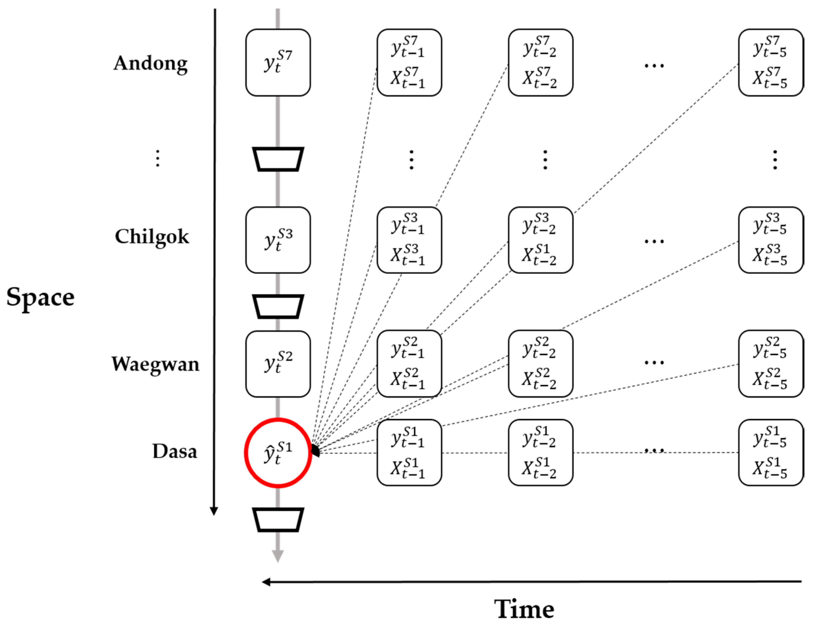
To predict the chlorophyll-a concentration in time step t at Dasa, we considered the time lag t − 1 to t − 5 and the site variables. Considering Dasa (S1) as the evaluation site, Figure 1a shows six monitoring sites upstream of Dasa: Waegwan (S2), Chilgok (S3), Dogae (S4), Sinam (S5), Hoesang (S6), and Andong (S7). Figure 2 shows how the response variables were predicted. The red circle denotes the prediction target, namely chlorophyll-a concentration in time step t at Dasa (${\widehat{y}}_t^{S1})$. The dotted arrows denote that the explanatory and time–lagged variables of each identified site affect the response variable.

Forward Selection

Using time–lagged variables as explanatory variables from time t − 1 to t − 5 for each site results in too many explanatory variables (approximately 366) (Figure 2). Thus, we used forward selection as the variable selection method. The forward selection method starts with a null model. Then, variables are added, if needed, to the model one by one, and the forward selection method calculates the p-value for each variable. These processes are repeated until all the variables that significantly affect the chlorophyll-a are found [9]. A critical threshold p-value of 0.05 was adopted in this study. The results of the forward selection showed that many variables had no relation with chlorophyll-a at Dasa and including them in our analysis would affect the prediction adversely. Accordingly, we structured the training data with the 14 most meaningful variables (

Table 2. Variables selected as a result of forward selection.

Variable	Estimate	Standard Error	t Value	p-Value
Intercept	1.110	0.258	4.304	<0.001
${\mathrm{Chla}}_{\mathrm{t}-1}^{\mathrm{S}1}$	0.862	0.014	60.009	<0.001
${\mathrm{RainFall}}_{\mathrm{t}-1}^{\mathrm{S}1}$	−0.011	0.003	−3.444	<0.001
${\mathrm{pH}}_{\mathrm{t}-5}^{\mathrm{S}5}$	−0.102	0.025	−4.100	<0.001
${\mathrm{SunShine}}_{\mathrm{t}-1}^{\mathrm{S}2}$	0.018	0.004	4.238	<0.001
${\mathrm{RainFall}}_{\mathrm{t}-2}^{\mathrm{S}3}$	−0.006	0.002	−3.989	<0.001
${\mathrm{Outflow}}_{\mathrm{t}-1}^{\mathrm{S}4}$	0.063	0.021	2.959	0.003
${\mathrm{TOC}}_{\mathrm{t}-1}^{\mathrm{S}2}$	−0.380	0.074	−5.158	<0.001
${\mathrm{TOC}}_{\mathrm{t}-1}^{\mathrm{S}4}$	0.049	0.014	3.574	<0.001
${\mathrm{TOC}}_{\mathrm{t}-3}^{\mathrm{S}7}$	0.199	0.054	3.665	<0.001
${\mathrm{Outflow}}_{\mathrm{t}-4}^{\mathrm{S}4}$	−0.054	0.020	−2.684	0.007
${\mathrm{Chla}}_{\mathrm{t}-4}^{\mathrm{S}7}$	−0.010	0.003	−3.034	0.002
${\mathrm{SunShine}}_{\mathrm{t}-4}^{\mathrm{S}3}$	−0.008	0.003	−3.066	0.002
${\mathrm{TOC}}_{\mathrm{t}-4}^{\mathrm{S}7}$	−0.137	0.053	−2.587	0.01
${\mathrm{TOC}}_{\mathrm{t}-4}^{\mathrm{S}2}$	0.189	0.073	2.589	0.01

).

2.2. Machine Learning Methods

In this study, we constructed a suitable chlorophyll-a prediction model for water quality management against algal blooms. We used various machine learning models, such as Support Vector Regression (SVR), Bagging, RF, XGBoost, RNN, and LSTM, to build the prediction model.

2.2.1. Support Vector Regression (SVR)

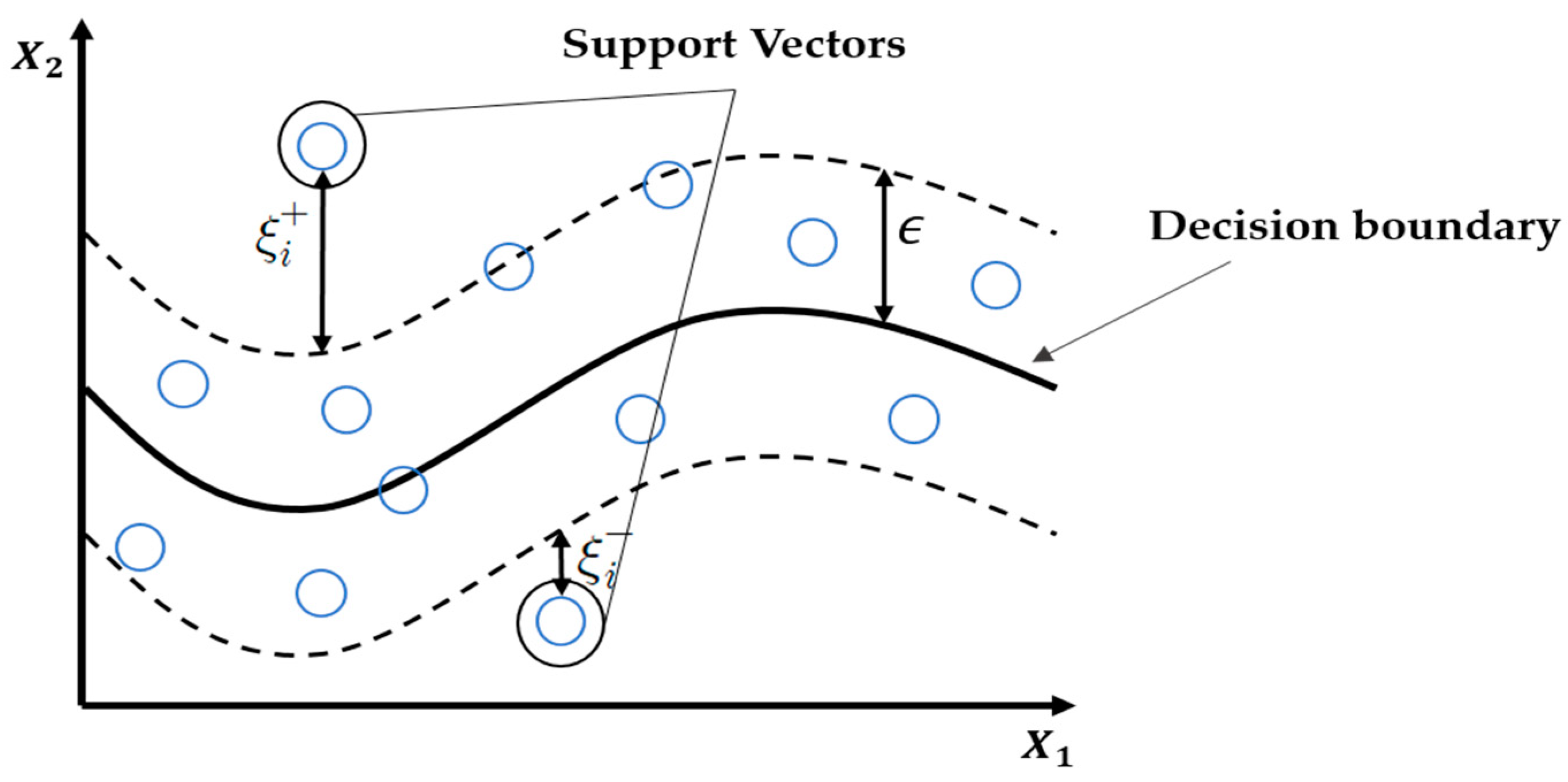
SVM were introduced in 1992 by Boser et al. [36]. SVMs are used in a wide range of fields, such as machine learning, optimization, statistics, and functional analysis [37,38]. The SVM concept can be generalized to become applicable to regression problems [39]. SVR, one of the applications of the SVM, finds hyperplanes that minimize the errors and maximize the margins of continuous data. In the following equation, minimizing the value of the left term $w$ is equivalent to finding a value that maximizes the margin (Figure 3).

$$\min {\left|\left|w\right|\right|}^2+C{\displaystyle \sum }_i^n\left({\xi }_i^{+}+{\xi }_i^{-}\right)$$

(1)

The term on the right-hand side of Equation (1), ${{\displaystyle \sum }}_i^n\left({\xi }_i\right)$, is an empirical error, and indicates the extent of error shown by the decision function for a given learning data set. Hence, the function in Equation (2) was used to minimize Equation (1) [40].

$$f\left(x\right)={\displaystyle \sum }_i^n\left({\alpha }_i^{*}+a_i\right)K\left(x, x_i\right)+B$$

(2)

$K\left(x, x_i\right)$ in Equation (2) is the kernel function, ${\alpha }_i^{*}$, $a_i$ ≥ 0 are the Lagrange multipliers, and $B$ is a bias term. The kernel trick is used to solve this SVR problem [41,42]. In this study, we built the best SVR model using a kernel function called the radial basis function. In summary, the purpose of the SVR is to find a value that maximizes the margin, while keeping the difference between the actual and predicted values lower than $ϵ$.

2.2.2. Ensemble Learning

Bagging (or Bootstrap Aggregation), RF, and boosting are similar in that they use ensemble learning, wherein several decision trees are combined to produce better prediction performance than that provided by a single decision tree [43].

Bagging

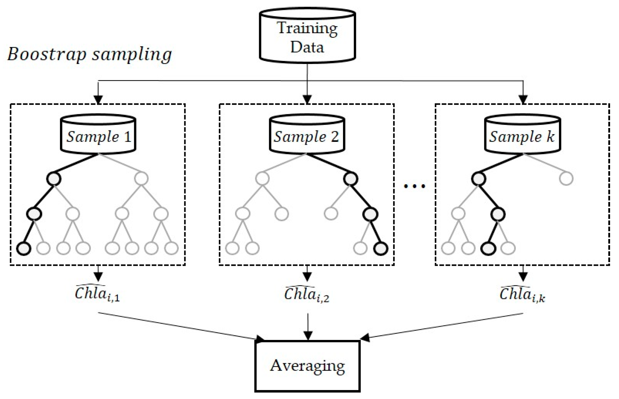
Bagging extracts bootstrap samples, such as the sub–training data, from the given training data and generates a prediction model for each item of the sub–training data [11]. This method uses the average of the prediction results outputted by each sub–model (Figure 4). The procedure for bagging is outlined below.

Step 1. Suppose N observations and M features. A sample from the observations is selected randomly with replacement.

Step 2. A subset of features is selected to create a model with a sample of observations and a subset of features.

Step 3. A feature is selected from the subset such that the best split of the training data is obtained.

Step 4. Step 3 is repeated to create multiple models, and every model is trained in parallel.

Step 5. A prediction is produced based on the aggregation of predictions from all the models.

Random Forest (RF)

Creating trees repeatedly via bagging results in a high correlation between the trees. To reduce this correlation, the RF selects random features from M features, and provides predictions based on the average of several trees generated by the feature randomization (Figure 5). In other words, RF adjusts the number of explanatory variables used in each decision tree model to statistically increase the independence of each model. This can significantly reduce the variability of the results and improve prediction performance [44].

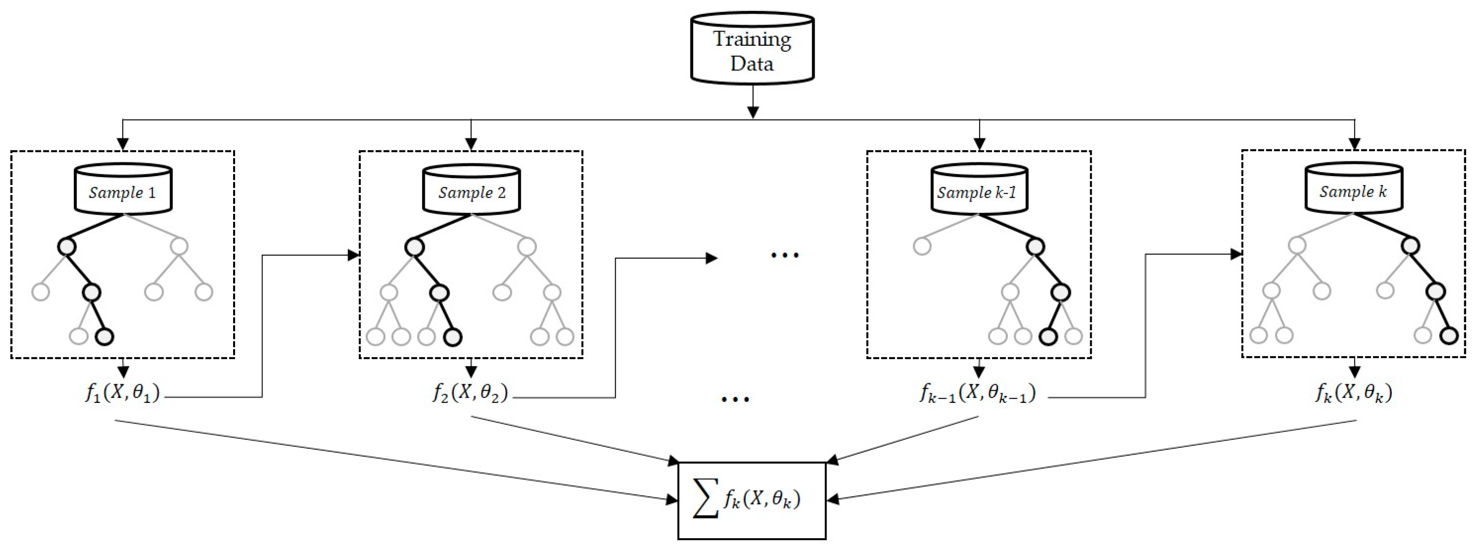
Extreme Gradient Boosting (XGBoost)

XGBoost is based on a model that assigns a higher weight to misclassified data using a gradient boosting method [45]. Boosting algorithm–based regression analysis, wherein each tree is based on a decision tree that is dependent on the previous tree, uses decision partitioning to generate step–by–step functionality (Figure 6). The specified loss function is optimized using the residuals from the previous tree [46].

When the first model is generated, the difference between the model predictions and observations is calculated (i.e., residuals or misclassifications) [11,45]. The different tree models can suitably predict the misclassification obtained in the first stage. The residuals remaining after the first two stages are matched to the other trees in the third stage, and the process is repeated several times.

The purpose of the model is simplification through optimizations of the training loss ($l$) and regulations ($\mathsf{\Omega }$). $f_k$ is the function of the K–tree. The objective function (J) in round t is given by Equation (3) [46].

$${\mathrm{J}}^{\left(t\right)}={\displaystyle \sum }_{i=1}^{n}l\left(y_i, {\widehat{y}}_i\right)+{\displaystyle \sum }_{k=1}^K\mathsf{\Omega }\left(f_k\right)$$

(3)

In this study, $y_i$ is the observed chlorophyll-a concentration at Dasa, and ${\widehat{y}}_i$ is the obtained final prediction value.

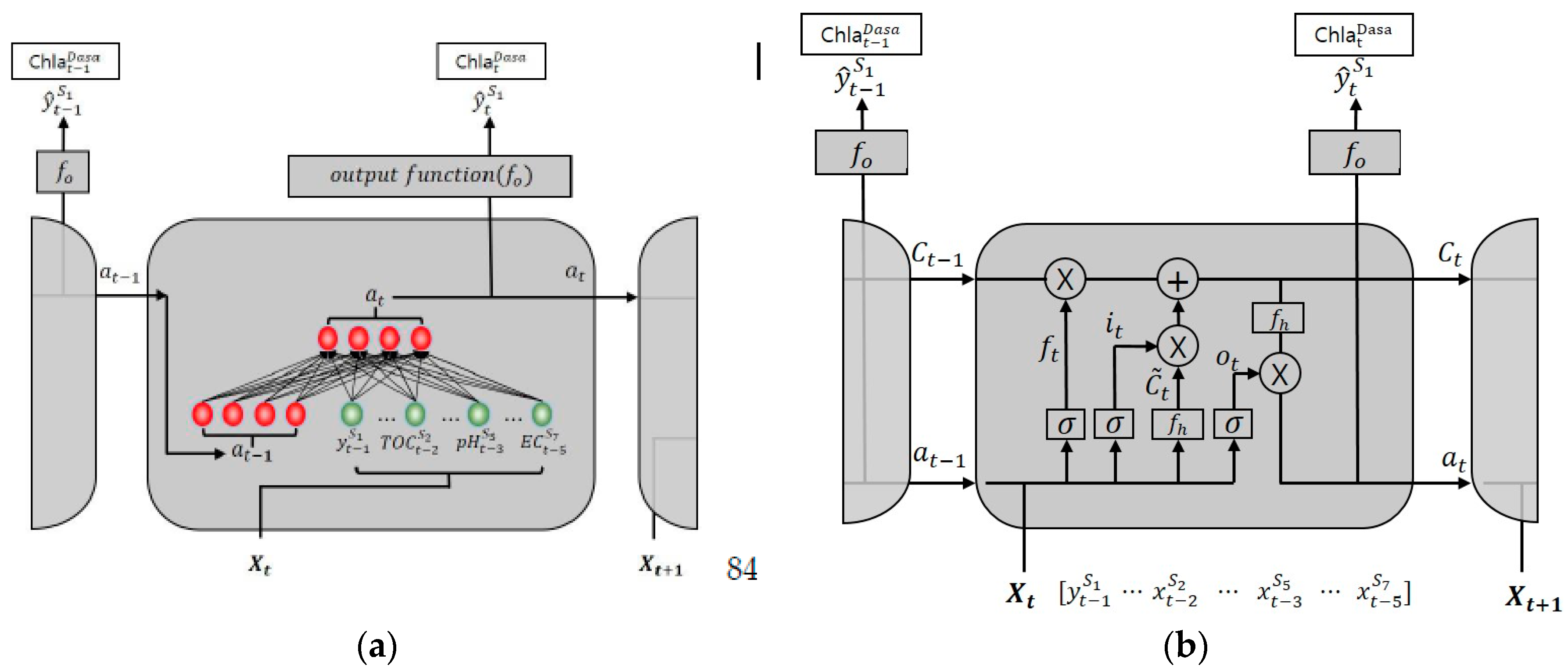
2.2.3. Recurrent Neural Network (RNN) and Long–Short-Term Memory (LSTM)

As water quality is judged using many variables that are nonlinear in nature, we require a neural network possessing the power to analyze nonlinear data [13]. RNN and LSTM can be used to predict future chlorophyll-a concentrations based on the present values of explanatory variables and past information; therefore, these models are widely used with time series data. Unlike feed–forward neural networks, RNN delivers information in both directions, and the calculation computed from the initial input is fed back to the network, which is critical in learning the nonlinear relationships between multiple water quality variables [47]. Figure 7a shows the structure of the RNN model; the hidden state $a_t$ at time t is computed as an activation function $f$ of the previous hidden state $a_{t-1}$, and the current explanatory variables ${\mathit{X}}_t$(${\mathrm{pH}}_{\mathrm{t}-5}^{\mathrm{S}5}$, ${\mathrm{TOC}}_{\mathrm{t}-5}^{\mathrm{S}2}$, ${\mathrm{Chla}}_{\mathrm{t}-1}^{\mathrm{S}1}$, etc.). The equation’s hidden state, $a_t$, is calculated using Equation (4). In the following equation, ${\mathit{W}}_1$ is the conventional weight between an input layer and the hidden layer, and ${\mathit{W}}_2$ is the matrix of recurrent weights between the hidden layer and itself at adjacent time steps [47]. In other words, the RNN can reflect the previous hidden state in the current time process.

$$a_t=f\left({\mathit{W}}_1{x}_t+{\mathit{W}}_2{a}_{t-1}\right)$$

(4)

Unfortunately for RNN, during the training of data with long sequences, the components of the gradient vector can decay or grow significantly. Vanishing gradient is a fundamental issue in such cases, and it is difficult for the RNN model to reflect distant past information.

LSTM solves the problem using the interactions of three gating units and one memory cell. In Figure 7b, the forgotten gate $f_t$ determines whether to reflect the previous hidden state $a_{t-1}$. The input gate $i_t$ controls the degree to which a new value flows into the cell. The memory cell $C_t$ can carry relevant information throughout the processing of the sequence [48]. The memory cell reflects the old state value $C_{t-1}$ by the ratio of the forgotten gate $f_t$, and the new state value ${\tilde{C}}_t$ by the ratio of the input gate. LSTM stores the previous state information in $C_{t-1}$, and uses it to determine the current state $C_t$. Finally, the output gate $o_t$, through which the output is received, serves to adjust the output of the value stored in the memory cell $C_t$. One disadvantage of the LSTM, however, is that the model has three gates; therefore, the number of weights and deviation terms required for learning are approximately four times larger. This leads to a long learning time and produces overfitting with less training data.

In the proposed water quality predictive model, we applied the RNN and LSTM models. To predict the concentration of chlorophyll-a at time step t, the input time series included data in the previous m time steps. In addition, each time step had n water quality and weather variables. Consequently, each explanatory variable of the RNN model can be interpreted as an m × n matrix [18].

In addition, to improve the model performance of the RNN and LSTM models, the role of the activation function and the gradient descent optimization algorithms is very important. In this study, we used the Leaky ReLU (Rectified Linear Unit) function as an appropriate activation function and used Adagrad (Ada Adaptive Gradient) instead of SGD (Stochastic Gradient Descent) to reduce the possibility of falling into the local solution.

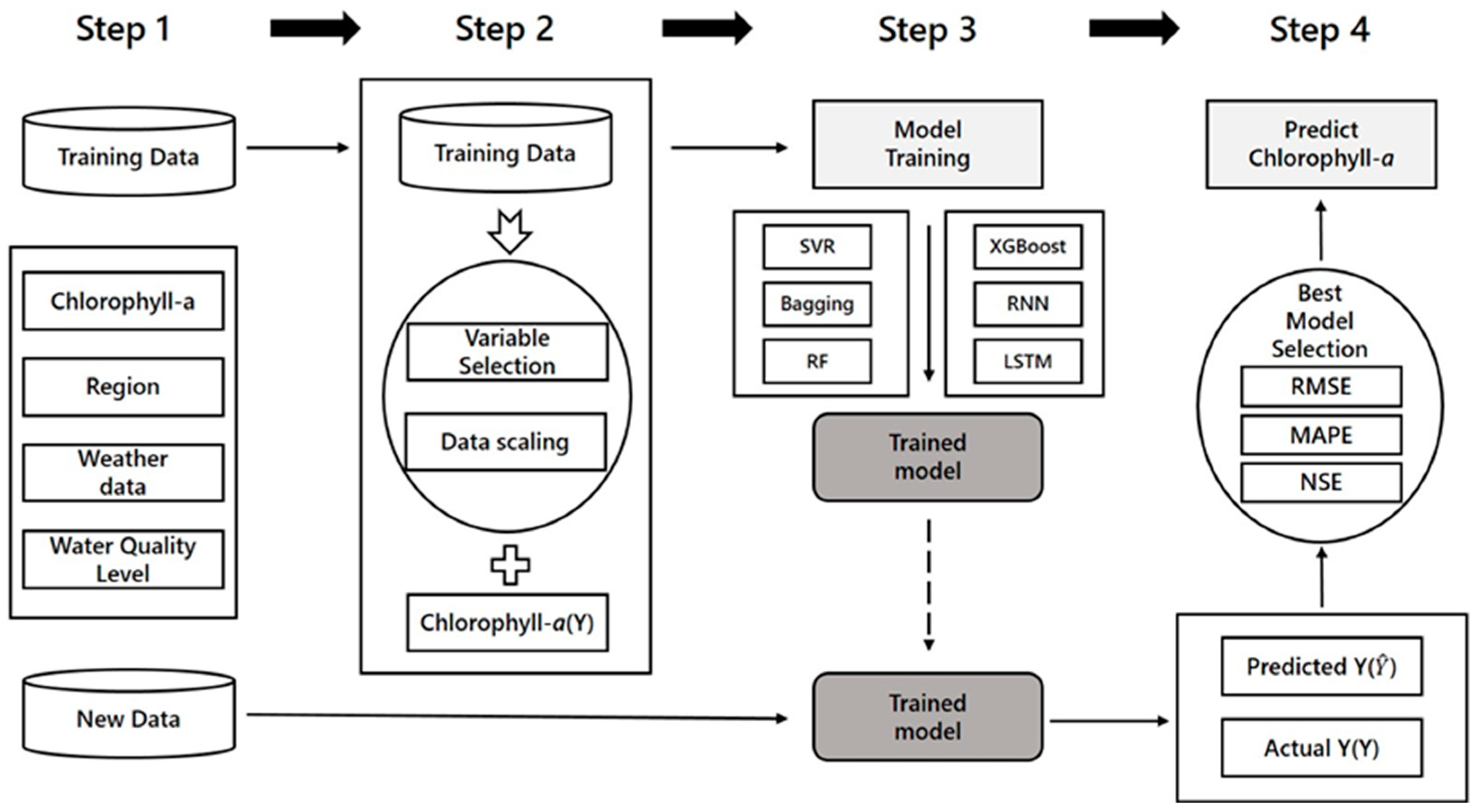
2.3. Workflow for Predicting Chlorophyll-a Concentration

The purpose of this study was to predict the chlorophyll-a concentration at Dasa using popular machine learning models. The collected data were divided into the training and test datasets (Figure 1b), and the training data were fitted into the various machine learning models described previously. The prediction procedures are summarized below, and Figure 8 presents the flow chart for the prediction of the chlorophyll-a concentration.

Step 1. Collect water quality/quantity data and weather data for each area, and divide them into training data for model fitting and test data to verify the model performance. In this study, daily data from June 2015 to November 2017 were used as the training data (891 d), and data from December 2017 were used as the test data (31 d).

Step 2. Preprocess the data. Since each variable has different units, it was necessary to perform data standardization that transforms the data such that the mean and standard deviation equal 0 and 1, respectively, and to select variables that best fit the model. Forward selection was used to select the significant variables.

Step 3. After preprocessing the data, fit the model using the selected variables via SVR, Bagging, RF, XGBoost, RNN, and LSTM.

Step 4. Predict the chlorophyll-a concentration levels in December 2017 using the fitted model, and compare it with the actual chlorophyll-a concentration levels in December. Root Mean Absolute Error (RMSE), Mean Absolute Percentage Error (MAPE), and the Nash–Sutcliffe coefficient of efficiency (NSE) were used as indicators to confirm the prediction accuracy. The indicator checks ensured that the model with the lowest RMSE and MAPE and the highest NSE value was selected as the optimal model. The optimal model parameters were determined by trial and error.

The number of data used for model testing were relatively small (approximately 3% of the training data), while the chlorophyll-a concentration in the test data ranged from 20.7 to 38.2 $\mathrm{mg}/{\mathrm{m}}^3$, covering 30% of the yearly chlorophyll-a concentration variation. Less than 5% of the data showed values higher than 38.2 $\mathrm{mg}/{\mathrm{m}}^3$ in 2017. Thus, the test period was considered to be representative of that year’s data variation and suitable for the model performance test.

2.4. Cross–Validation and Model Accuracy Metric

To improve the performance of machine learning prediction models, the process of finding the optimal model parameters is very important [25]. In this study, the cross–validation method was used to determine the optimal combinations of the hyper–parameters of the proposed models. The following hyper–parameters were considered: learning rate, number of hidden nodes, and batch size for RNN and LSTM; C and sigma for SVR; and number of trees for the ensemble models (Bagging, RF, and XGBoost). Note that RF adds the number of features to hyper–parameter, while XGBoost adds tree complexity to hyper–parameter.

Uncertainty evaluation in time series prediction models are based on chlorophyll-a concentration observations [49]. In this study, the prediction performance of the model was compared using the following three indicators: RMSE, MAPE, and NSE [49].

$$RMSE=\sqrt{\frac{1}{n}{\displaystyle \sum }_{i=1}^n{\left(y_i-{\widehat{y}}_i\right)}^2}$$

(5)

$$MAPE=\frac{1}{n}{\displaystyle \sum }_{i=1}^n\frac{|y_i-{\widehat{y}}_i|}{y_i}\times 100$$

(6)

$$NSE=1-{\displaystyle \sum }_{i=1}^n\frac{{(y_i-{\widehat{y}}_i)}^2}{{\left(y_i-\overline{y}\right)}^2}$$

(7)

where $y_i$ denotes the observed value (chlorophyll-a at Dasa), $\overline{y}$ is the average of observed value, and ${\widehat{y}}_i$ refers to the value predicted by the model. The smaller the RMSE and MAPE and the higher the NSE, the better the prediction performance of the model.

2.5. Model Validation

The model validation step evaluates the performance of a model built using the various methods. For the model validation in this study, we divided the data into a training set, which was used for the model construction, and a test set, which was used to evaluate the model performance by measuring its accuracy on unseen data. The hold–out method is simple; the original dataset is randomly divided into the training and test datasets. Typically, 80% of data are used for training, and the remainder (20%) for testing.

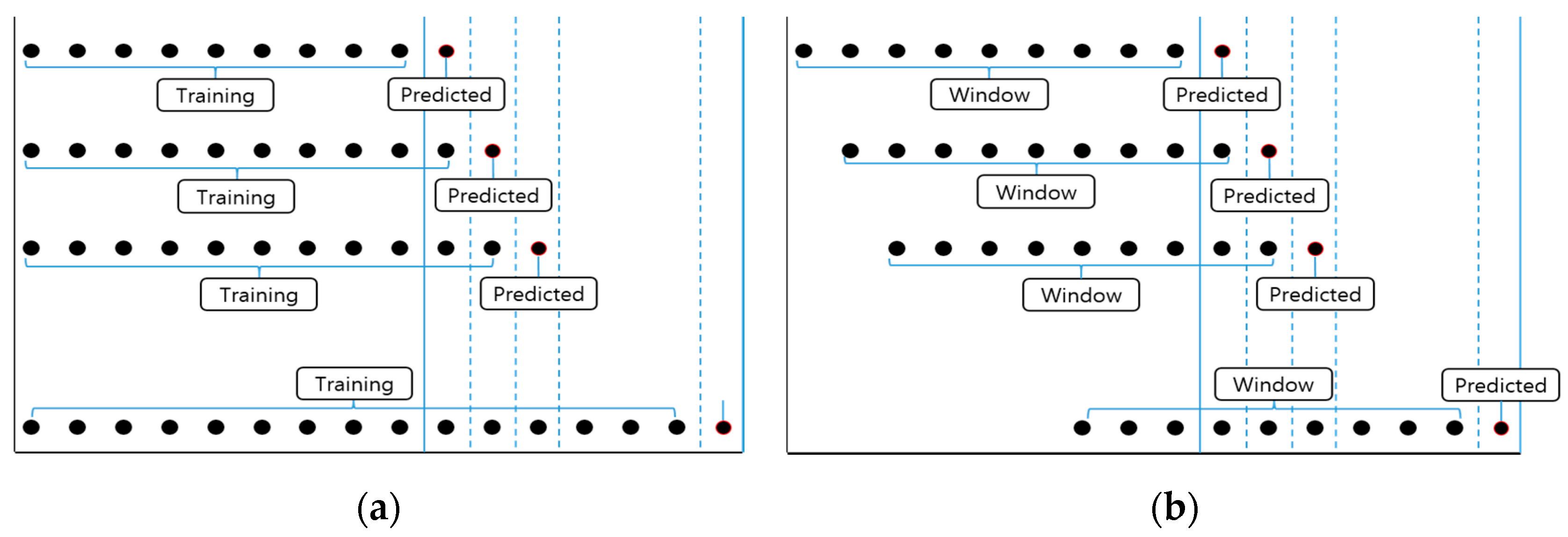
In this study, we used 1–step ahead recursive prediction to reflect the characteristics of the time series. This method adds the input data to the model in a stepwise fashion when constructing it for future prediction [47]. We used cumulative learning and rolling window learning for this purpose.

Cumulative learning is performed as follows: construct a model using the data at time point t and predict the future value at time t + 1. After adding the data at time t + 1, build the model to use data at [1, ..., t + 1] to predict the value at time step t + 2. After this process is repeated and when predicting the value after time N has elapsed, construct the model using data from the time step [1, ..., t + 1, ..., t + N], and predict the value at time step t + N + 1. (Figure 9a). In this study, the size of t (as per the number of training data) was 891, while N (the number of test data) equaled 31.

Rolling window learning uses a process similar to that of cumulative learning. Construct a model using the data at time point t, and predict the future value at time t + 1. After adding the data at time t + 1, use the data at [2, ..., t + 1] to build the model to predict the values at time step t + 2. After this process is repeated, to predict the value after time N construct the model using data from time step [N + 1, ..., t + 1, ..., t + N], and then predict the value at time step t + N + 1. In this case, the data of a certain section used for building the model are called a window, and the size of the window in the above example is t. In addition, the size of the window can be freely adjusted (Figure 9b). In this study, the prediction was performed by fixing the window size to 891.

We used R (version 3.5.1), a software environment for statistical computing and graphics.

3. Results

Table 3. Prediction performance of the studied machine learning models.

Method		1–Step Ahead Recursive Prediction
		Cumulative Learning			Rolling Window Learning
		MAPE (%)	RMSE	NSE	MAPE (%)	RMSE	NSE
All variables	SVR	11.02	3.864	0.5308	11.12	3.8950	0.5233
	Bagging	28.58	10.41	−2.4049	33.88	11.6356	−3.2545
	RF	16.53	5.760	−0.0426	16.23	5.5398	0.0356
	XGBoost	8.69	3.5854	0.5960	09.16	3.6702	0.5767
	RNN	11.28	4.2872	0.1765	15.88	5.4196	−0.1164
	LSTM	16.38	5.8634	0.2136	14.15	5.2502	−0.1653
Selected variables based on forward selection	SVR	9.85	3.1717	0.6838	9.85	3.1750	0.6832
	Bagging	16.33	6.3604	−0.2712	13.37	4.9668	0.2247
	RF	8.50	3.1213	0.6939	8.98	3.1920	0.6798
	XGBoost	10.21	3.9305	0.5145	9.53	3.7712	0.5531
	RNN	7.54	2.6843	0.7601	7.27	2.6453	0.7516
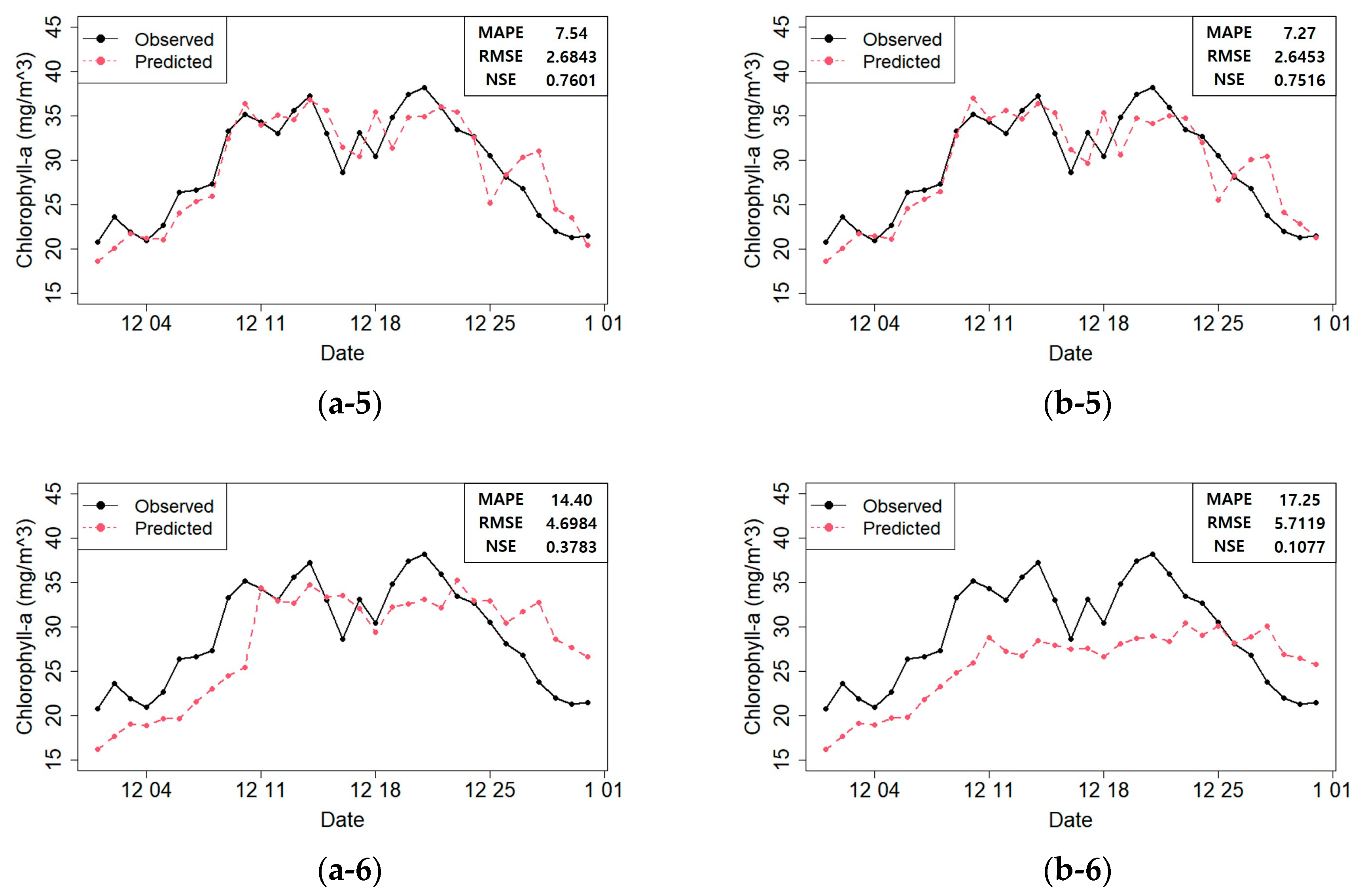
	LSTM	14.40	4.6984	0.3783	17.25	5.7119	0.1077

compares predicted and actual values using the six previously mentioned models (SVR, Bagging, RF, XGBoost, RNN, and LSTM) built with all the variables; and with only the selected variables. Cumulative learning and rolling window learning were used for the predictions. The results show that RNN outperformed the remaining machine learning models. In particular, the model obtained after building the training data with the selected variables and making predictions using rolling window learning showed the lowest MAPE and RMSE and the second highest NSE (MAPE: 7.27%, RMSE: 2.6453, and NSE: 0.7516).

The rolling window learning increased the prediction performance of each model. However, when the prediction used all the variables, the rolling window learning and cumulative learning did not show a significant performance difference. Moreover, in most cases, the models that used only the selected variables outperformed those that applied all the variables.

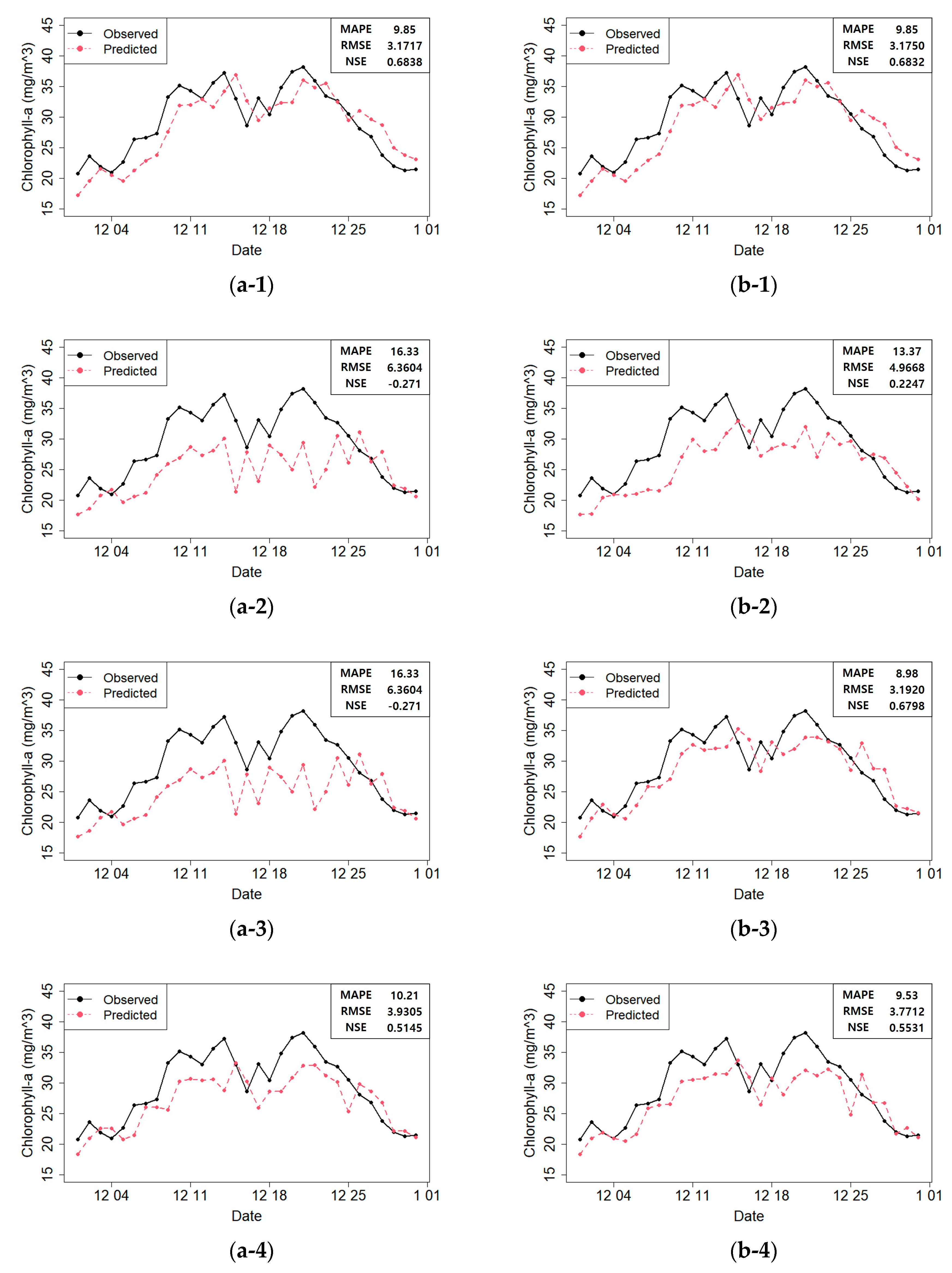
Figure 10 shows the predicted and actual values of the chlorophyll-a concentrations according to the model constructed with the selected variables.

Figure 10 shows that the prediction performances were acceptable in most cases. However, some models produced unreliable results in the prediction plot. For instance, the RF and SVR prediction plots showed that the actual value at time t − 1 and the predicted value at time t were very similar. This phenomenon can be attributed to the fact that the chlorophyll-a concentration at time t − 1 correlated too strongly with the response variable in time step t at Dasa. Therefore, the RF and SVR model predictions were unreliable. On the contrary, in the RNN prediction plot (b–5; Figure 10), this phenomenon was minimized, and the predicted values matched the actual values well. Moreover, the fitted models did not perform well after December 25th (Figure 10). We found that heavy rainfall had occurred along the course of the Nakdong River on December 24th, which must have affected the result. Therefore, in the future, we plan to construct a more accurate prediction model that can reflect such special events.

4. Discussion

A recent study that predicted chlorophyll-a concentrations in regions characterized by a monsoon–like climate indicated that SVM provides the highest prediction performance [50]. However, our study used an RNN model to reflect the temporal characteristics of the data for prediction purposes, and showed better prediction results than the other machine learning models, including SVM. Another previous work that predicted chlorophyll-a concentrations in the four major rivers of South Korea reported that RNN and LSTM showed better prediction performance than the Multilayer Perceptron and Ordinary Least Squares approaches, but the prediction accuracies were not high [32]. In contrast, our study used variable selection and 1–step ahead recursive prediction to improve the prediction performance of RNN.

This study increased the prediction accuracy of future chlorophyll-a concentrations in several ways. First, the remarkable prediction performance of RNN can be attributed to its innate ability to interpret temporal characteristics better than other models (SVR, Bagging, RF, and XGboost), and a previous study also showed relatively poor prediction performance by the other models [32]. However, LSTM showed lower prediction performance than commonly used machine learning models. This may have resulted from overfitting because the LSTM structure tends to be more complex and requires more data. The increase in data availability could further improve the accuracy of more complicated machine learning models such as LSTM. Thus, it is expected that advanced machine learning models will provide better predictions of the variable of interest and assist the real–time management and automated operation of drinking water supply systems in the near future. Second, machine learning modeling via variable selection showed improvements in prediction performance [27]. Third, cumulative learning and rolling window learning increased the prediction performance of each model [47]. However, significant differences in the performance of most machine learning models were not evident between these two approaches. Therefore, the process of improving model performance is important; to this end, we applied two techniques: 1–step ahead learning (depending on the type of machine learning model) and forward selection (depending on the characteristics of the data). Fourth, to improve the prediction performance, the previous time variables from upstream sites were used as explanatory variables for the predictions. In Figure 1b, the chlorophyll-a concentration trend at each site follows a similar pattern, indicating correlations with each other. Moreover, Table 2 shows that the explanatory variables from the previous time (t − 1 to t − 5) at each site significantly affect the chlorophyll-a concentration at Dasa at time t. In particular, TOC, an indicator of organic pollution, shows a clear correlation with chlorophyll-a concentrations, which means that the water quality at previous times at each site and the current chlorophyll-a concentrations are strongly correlated. The results of the present study concur with those of previous works involving a lake in South Korea [2,4].

The prediction of algal blooms in freshwater systems can provide useful information for the proper management and operation of drinking water supply systems. For example, the operator can plan for additional treatment processes, such as activated carbon treatment, when an increase in the algae concentration in the water source is expected. However, the prediction of algal blooms is a difficult task, as algal growth in freshwater systems is affected by various physical, chemical, and biological processes. The effects are not easily quantifiable in rivers and lakes; in general, rainfall in watersheds causes an increase in the pollutant load, leading to a consequent rise in algal growth, whereas a decrease in algal concentration is expected by washout in the short term. The machine learning models used in this study predicted chlorophyll-a concentrations based on the relationships among the observed data rather than the physical, chemical, and biological mechanisms of algal growth.

Our study obviously suffers from some limitations which should be addressed in future work: (a) There might be multicollinearity causing overfitting problem because the water quality variables used in this study are closely related to each other. (b) Despite the fact that the ensemble technique has the advantage of improving accuracy, this study has the limitation that it is not possible to evaluate the uncertainty of weight in the results. Thus, further investigations should be performed to overcome these limitations. Possibly applicable methods are to utilize regularization techniques such as ridge, lasso, and elastic net to solve overfitting problem in (a), and apply Bayesian Model Averaging (BMA) to model uncertainty in (b).

5. Conclusions

This study constructed and tested different machine learning models for chlorophyll-a prediction at Dasa weir, the Nakdong River, Korea. The RNN model outperformed the other models (SVR, Bagging, RF, XGboost, and LSTM). Our results showed that variable selection using the forward selection method and predictions using the 1–step ahead recursive learning can increase machine learning model prediction accuracy. Water quality at previous times at sites upstream of Dasa weir influenced the current chlorophyll-a concentration at Dasa. Moreover, the results of our study suggest that our overall technique can be successfully generalized to make chlorophyll-a predictions at other river sites.