Experimental and Numerical Assessment of Water Leakages in a PVC-A Pipe

Abstract

Nowadays, in the definition of effective approaches for the sustainable management of water pressurized systems, the assessment of water leakages in water supply and distribution systems represents a key aspect. Indeed, the large water volumes dispersed yearly provoke relevant environmental, technical and socio-economic costs. Worldwide, many water systems show alarming levels of water losses, due to both the poor sealing of joints and the presence of cracks, enhanced by a high pressure level greater than that strictly required for assuring a proper service level to users. With the aim of analysing the correlation between pressure and leakages, in this work the results of an experimental and a numerical Computational Fluid Dynamics (CFD) investigation are provided and discussed. With reference to a drilled PVC-A (Polyvinyl Chloride-Alloy) pipe, a new-generation plastic material for water systems use, an experimental investigation was first carried out at the Laboratory of Hydraulics of the University of Naples Federico II, aimed at assessing the leakage-pressure relation for transversal rectangular orifices. A CFD model was then implemented and calibrated with experimental results, to different geometric configurations of the orifice, with the aim of assessing the dependence of the orifice geometry and orientation on the calibration of leakage law parameters.

1. Introduction

During the last decades, the growing water demand coupled with climate change and anthropization are encouraging the development of effective approaches for the monitoring and management of water systems. In Italy, Water Supply Systems (WSSs) and Water Distribution Networks (WDNs) often present significant water losses, related to the poor infrastructure maintenance and the generally high system pressure. Water losses in supply systems and urban distribution networks cause major concern for communities and water utilities worldwide. Indeed, the so-called Non-Revenue Water (NRW) is responsible for significant economic damage to the management bodies, basically due to the lower income and to the increase of both operational and capital costs. In addition, water losses induce a variety of other effects, including: (i) social detriment due to service disruptions, damage to buildings and structures, traffic disturbance for unplanned maintenance; (ii) environmental impact caused by the increased abstraction of water from the natural cycle, the higher energy consumption and the possible alteration of groundwater flows; (iii) public health concerns related to increased exposure to the risk of contamination from backflow.

The water losses are mainly classified in “real (or physical) losses” and “apparent losses”. The former (e.g., the actual water leakages) can be classified into the following categories [1]: the background losses (e.g., those from leaking joints) and the burst pipes (reported and unreported), which correspond to significant pipe failures and whose manifestation is more or less immediate depending on the type and the entity of the damage. The “apparent losses” are mainly composed of revenue meter under registration, unauthorized consumption due to water theft and billing errors, instead.

With specific reference to the real losses, research efforts have been mainly focused on the hydraulic characterization of pipe burst events, due to their significant impacts on the economic and operational management of water systems. Therefore, the most viable strategy for leakage control is mainly focused on the system pressure and energy control [2,3,4]. Thus, for estimating the water losses deriving from pipe burst events, hydraulic characterization of the leakage is required, such as the relation between the leak outflow and the hydraulic head, the geometric features of the hole and the mechanical characteristics of the pipe.

From a theoretical viewpoint, water leakage originating from a burst pipe can be assimilated into an orifice flow, which is regulated by the well-known Torricelli’s equation [5,6]:

$$Q=C_L{A}_L\sqrt{2gH}$$

(1)

where $Q$ is the outflowing flow (m³ s⁻¹), $C_L$ is the flow coefficient (dimensionless), $A_L$ is the area of the leak (m²), $g$ the gravitational acceleration (ms⁻²) and $H$ is the driving pressure (m). Equation (1) properly emphasizes the clear dependence of the leakage on the water pressure; nevertheless, it has been proved to be not properly reliable in explaining experimental results obtained through field studies and laboratory tests [7,8] with reference to specific pipe materials.

Therefore, alternative formulations of the so-called “Leakage Law” (i.e., the pressure-leakage relationship) can be found in scientific literature. The most general expression is the monomial form provided by Lambert [5]:

$$Q=C{H}^N$$

(2)

where $C$ and $N$ are the leakage coefficient and exponent, respectively. An alternative approach is represented by the FAVAD (Fixed and Variable Area Discharge) concept, in which the bias between experimental data and predicted values of leaking discharge is explained assuming a linear deformation of the area of the leak with the pressure variations [9]. The FAVAD equation has the same structure as Equation (1), but it is specified as follows:

$$Q=C_D{A}_0\sqrt{2g}·\left[H^{\nu }+A{H}^{1+\nu }+B{H}^{2+\nu }\right]$$

(3)

with

$$A=\frac{\rho ·g·\left({\delta }^2+2\right)}{E({\delta }^2-1)}$$

(4)

$$B=\frac{{\rho }^2·g^2·\left({\delta }^2+1\right)}{E^2·{({\delta }^2-1)}^2}$$

(5)

being: $C_D$ the flow coefficient (usually set between 0.57 and 0.60), $A_0$ the initial area of the leak, $\rho$ the water density, $g$ the acceleration of gravity, $\delta$ the ratio between the internal and outer radius of the pipe, and $E$ the modulus of elasticity of the pipe material.

Most of the research studies carried out so far have addressed the characterization of the parameters of the leakage laws for different pipe materials and shapes and sizes of the cracks [10,11,12,13,14,15]. Specifically, it has been observed that the coefficient $C$ of Equation (2) increases almost linearly with the area of the crack, which is consistent with the other reported formulations. Much more uncertainty affects the estimation of $N$, for which different values in a very large range have been detected (from ~0.50 up to ~2.79).

Nevertheless, Franchini and Lanza [16] pointed out that the significant deviations of $N$ from the theoretical value may be basically ascribed to the improper quantification of the leakage coefficient $C$. Through a dimensionless analysis, the authors emphasized the effectiveness of the Torricelli’s equation in describing the pressure-leakage relationship and proposed that the influence of hydraulic factors and of the local deformability of the leak area is explained through the correction of the product $C_L{A}_L$ by means of a multiplicative factor. De Paola and Giugni [14] carried out an experimental comparison between steel and ductile iron pipes considering orifices with different shape and size. Both static and dynamic operations were simulated, pointing out how the emitter coefficient C strictly depends on the orifice size, whereas the leakage exponent N tends to a value close to the theoretical one of 0.50. At the same time, exponent coefficients significantly higher than 0.50 were observed for highly corroded steel pipe, asbestos cement and plastic pipes with longitudinal cracks, with reference to a real water district by Greyvenstein and van Zyl [12]. Specifically, they observed the leakage exponent varying from 1.38 to 1.85 for PVC-U pipes, whereas values in the order of 0.79–1.04 were detected for asbestos cement, instead. On the contrary, for a circumferential crack, typical values from 0.41 to 0.53 were determined.

In addition, for metallic pipes, corrosion has been observed to reduce the material mechanical properties around the leak, with significant effects on the leakage coefficient. Similar behaviour was observed for plastic pipes, which suffered from high elasticity, instead [6,16,17].

Ferrante et al. [17] observed how the visco-elastic nature of polyethylene pipes affects the leak outflow, giving rise to a hysteretic behaviour. Indeed, the water losses were observed to depend not only on the synchronous total head but also on its history and variation rate. Such behaviour is better modelled by the FAVAD equation (Equation (3)), accounting for the orifice deformation caused by pressure variation [8,13,18].

With specific reference to HDPE (High-Density Polyethylene) pipes, experimental studies have investigated the visco-elastic nature of the material [17,18,19], responsible for the hysteretic behaviour exhibited in tests with cyclic pressure load. van Zyl and Clayton [11] and De Paola et al. [20] experimentally assessed the interaction between leakage and surrounding soil, analysing the potential influencing factor of the leak detection.

The development of mitigation strategies, as well as the identification of the “economically recoverable” water losses (e.g., the losses for which investments in corrective actions have a reasonable payback period), strictly requires a proper estimation of the amount and the location of the water leakages [21,22,23]. Nevertheless, an important contribution can be provided by hydraulic modelling, which can be used to both locate the leaks and investigate the effectiveness of mitigation actions based on the physical and operating data of the water system. Of course, the calibration of the hydraulic models to actual field data is essential to achieve realistic and usable results [24]. In this context, laboratory calibration of leakage law parameters has a pivotal role, allowing the leaking water volume to be accurately estimated.

In addition to experimental assessment and hydraulic modelling, Computational Fluid Dynamics (CFD) models represent a useful tool to simulate the hydraulic behaviour of leakages in water systems, with reference to different operational scenarios and pipe materials [25,26,27]. Cassa and van Zyl [25] investigated the relationship between pressure head and leak area in pipes with longitudinal, spiral and circumferential cracks, observing a linear relationship between crack area and pressure for all the investigated crack types, pipe materials and pressure. Shehadeh and Shahata [26] numerically assessed different rupture diameters of steel pipe, varying both the pressure and the flow rate. They observed a direct correlation between maximum velocity, total pressure, turbulence intensity and leakage mass-flow rate with the rupture area in pipes. Danesh and Assan [27] numerically calibrated the discharge coefficient for different orifice diameters and pipe diameter ratios and compared the results with experimental observations. CFD simulations were also applied to track the vena-contracta downstream of the orifice [28].

The availability of new material and technologies for pipe production, together with their increasing adoption in the design of WDNs, calls for a proper hydraulic characterization in terms of leakage law. Indeed, from the technological perspective, as reported by Scott [29], the principal manufacturers of PVC (Polyvinyl Chloride) pipe systems have developed and enhanced the performance of the product, combining thinner wall thickness and lower weight, together with an improved ductility and performance. Among the variety of improved performance PVC pipes, PVC-A (PVC-Alloy) pipe systems are gaining increasing interest. The hydraulic behaviour, in terms of leakage law, is still unexplored for these pipes. The PVC-A manufacturing process involves the combination of an impact-resistance modifier (CPE, chlorinated polyethylene) with the basic PVC. The CPE ensures that the pipe has improved toughness and ductility, whilst reducing the wall thickness by approximately 30% when compared to standard PVC [29]. Its main advantages stem from the significant stability of PVC-U (unplasticized PVC) and the plasticity conferred by Polyvinyl Chloride, at the same time providing great resistance and interesting flexibility. The PVC-A is increasingly applied to no-dig (or trenchless) technologies, suitable for both pressurized and gravity water systems, thanks to the junction system with a gasket that confers an effective hydraulic seal over time. Furthermore, the polymeric alloy provides high resistance to crack propagation, guaranteeing a longer product life and lower maintenance interventions, beyond the excellent resistance to electrochemical corrosion.

Owing to the mentioned mechanical and hydraulic properties, PVC-A represents a viable alternative relative to other pipe materials generally used in pressurized water systems, such as HPDE, steel and cast-iron. The assessment of leakage behaviour on new manufacturing pipes is thus of high interest, extending the knowledge about the leakage behaviour of a wide set of pipe materials for water supply and distribution services.

With the aim of overcoming the lack of knowledge about the mechanical response of PVC-A pipes to the generation of orifices and cracks, in this paper, results from an experimental and numerical analysis are discussed with reference to a PVC-A pipe presenting an artificially drilled bore, simulating the effects of a pipe burst event, with a transversal rectangular-shaped orifice. A total of 42 static tests were performed varying the flow rate from 10 L/s to 30 L/s and pressure from 1 to 7.5 bar. The experimental results were used to calibrate a numerical CFD model, implemented with the aim of exploring the dependence of water losses on the orifice size and orientation in PVC-A pipes. Four geometric configurations of the orifice were then simulated: (1) a transversal rectangular orifice, equal to that drilled on the experimentally investigated pipe; (2) a longitudinal rectangular orifice having the same area of the previous one; (3) a circular orifice with same area; (4) an irregular longitudinal crack.

In Section 2 the experimental setup and the CFD numerical model are presented; in Section 3 the discussion of results is provided, and the final considerations are presented in the Section 4.

2. Materials and Methods

2.1. The Experimental Investigation of the PVC-A Pipe

The experimental analysis was carried out at the Laboratory of Hydraulics of the University of Naples Federico II. The investigated pipe consisted of a 3.20 m long DN140 PVC-A pipe, manufactured by FITT Bluforce, fitted along steel instrumented DN125 pipeline. The geometrical and mechanical properties of the tested PVC-A pipe are summarized in

Table 1. Main features of PVC-A (PVC-Alloy) tested pipe.

External Diameter (mm)	Thickness (mm)	Pipe Length (m)	Young’s Modulus (kg/cm2)	Unit Weight (kg/m3)	Nominal Pressure (bar)
140	3.90	3.20	26,000	1400	10

.

The pipe was installed downstream of an air vessel as to obtain a driving pressure P varying from 1 up to a maximum of 7.5 bar, approximately. To assure a stable condition of supply, the flow was conveyed into the experimental pipe through a steel DN800 pipe (Idrogroup s.r.l., Naples, Italy), on which an air venting valve was installed. This pipe was linked to a pressure gauge to monitor the head upstream to the investigated PVC-A pipe. Specifically, a pressure transducer (S-11, WIKA Italia s.r.l., Milan, Italy, accuracy ± 0.25% of full scale) was installed on the upstream section, working in the range 0–10 bar by outputting a current signal between 4 and 20 mA.

A gate valve installed downstream to the DN800 pipe was employed to cut off the experimental pipe from the air vessel. The water supply was ensured by water volumes stored in underground tanks, by means of a recirculating pumping system. Specifically, the pumping system was composed of a 2-pole horizontal axis centrifugal pump (Omega 080-270, KSB Italia S.p.A., Monza, Italy), electrically connected to an inverter, able to vary its rotational speed N in the range 300–3000 rpm.

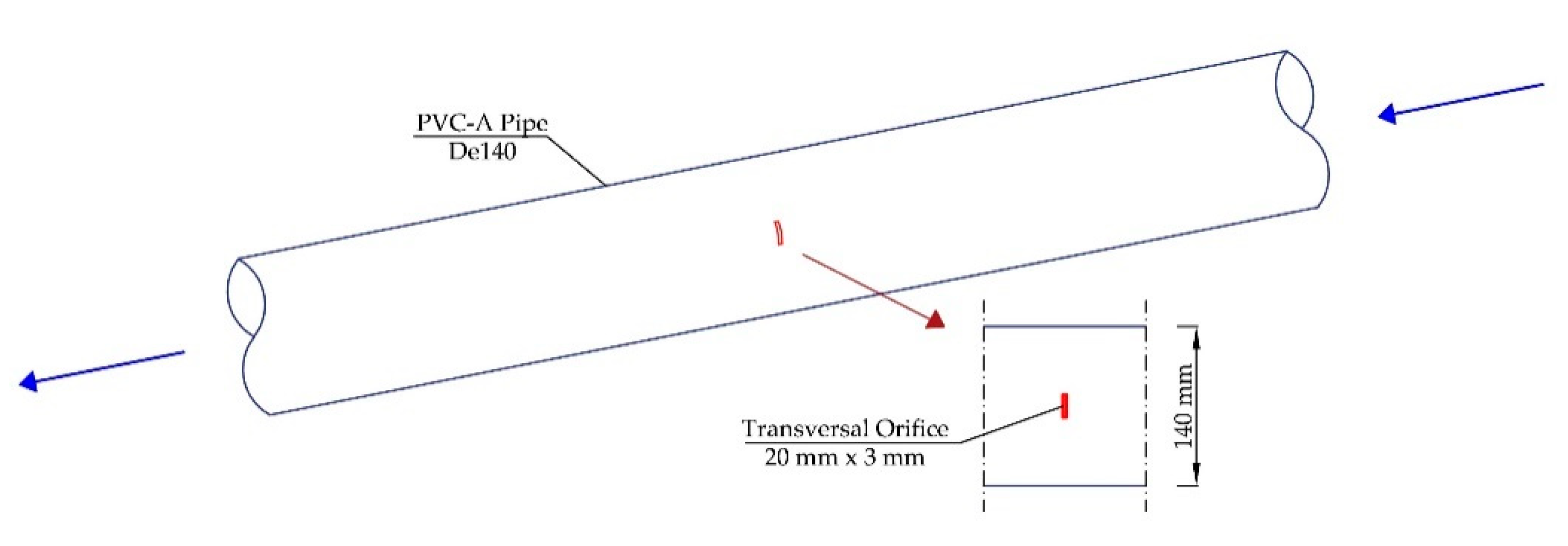
To simulate a leak on the pipe, a rectangular orifice of 20 × 3 mm was realized in the bottom side of the pipe, oriented transversally to the flow direction (Figure 1).

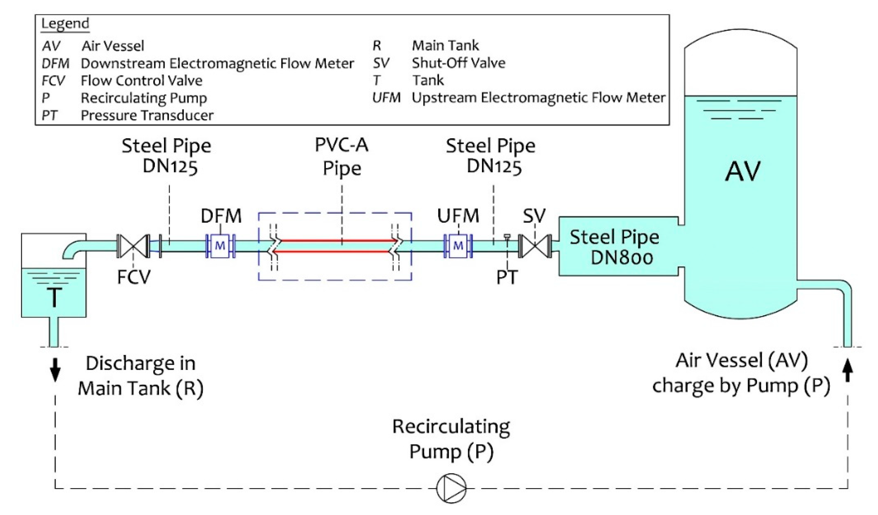
The leak discharged into a free surface tank connected to the recirculating system of the laboratory. At the downstream end of the pipe, a steel DN125 trunk with a needle valve (SAR. 07.6-F10, AUMA Italiana s.r.l., Milan, Italy) was installed, which conveyed the water to a recirculation tank, allowing the regulation of flow rate during the experiments. On the steel logs upstream and downstream of the PVC-A leak trunk, electromagnetic flow meters (SIMENS SITRANS MAG 5100W, Maddalena S.p.A., Udine, Italy, accuracy ±0.2% of full scale) were flanged. The experimental setup is schematically depicted in Figure 2.

To ensure the signal stability of the pressure transducer supply current, a power supply with an output voltage adjustable up to 30 V was installed. Nevertheless, considering the range of electric currents to be measured and the resistances added to the circuit, during the experiments a constant voltage of 20.7 V was set. All these devices were then connected to an acquisition system for data post-processing through a PC, so as to record the upstream and downstream flow rates, and the pressure head, with 2.0 Hz frequency. LJLogM^TN software (LabJack, Lakewood, CO, USA) was employed to elaborate the analogical signal sent via an acquisition card to the PC (Intel(R) Core (TM) i7-4720 HQ 2.60 GHz; 16 GB RAM). Preliminary calibration of the pressure transducer and the flow meters was performed, deriving the linear regression functions between the current intensity signal (mA) and the considered physical entity.

In order to simulate the typical nightly operations of a WDN, 42 static tests were performed. Indeed, during the night, an approximately constant pressure level is generally observed as a consequence of the low user demand. At each test, the static pressure was achieved by completely opening the upstream gate valve and varying the flow rate through the downstream needle valve. The static tests were performed with fixed flow rate Q_in and pressure P in the range 1–7.5 bar, according to the allowable operative range of the laboratory set-up. Three groups of tests were performed: (1) Q_in = 10 L/s ± 1 L/s; (2) Q_in = 20 L/s ± 1 L/s; (3) Q_in = 30 L/s ± 1 L/s (

Table 2. Set of performed experimental tests.

Qin = 10 L/s			Qin = 20 L/s			Qin = 30 L/s
TEST ID	P (bar)	Qin (L/s)	TEST ID	P (bar)	Qin (L/s)	TEST ID	P (bar)	Qin (L/s)
1	1.285	10.788	15	1.154	20.015	30	1.070	29.717
2	1.487	10.794	16	1.188	20.626	31	1.566	29.683
3	1.956	10.064	17	1.667	20.712	32	2.050	29.816
4	2.171	11.354	18	2.038	20.748	33	2.459	30.048
5	3.046	9.873	19	2.503	20.436	34	2.925	30.169
6	3.568	10.605	20	2.526	19.969	35	3.560	30.833
7	3.922	10.020	21	3.065	20.643	36	3.888	30.742
8	4.639	10.237	22	3.491	20.162	37	4.361	30.921
9	4.639	10.237	23	3.873	20.034	38	5.013	29.863
10	4.904	10.021	24	3.990	20.330	39	5.607	30.500
11	5.600	11.432	25	4.766	20.116	40	6.096	29.943
12	5.966	10.074	26	5.224	20.814	41	6.382	30.067
13	6.563	10.578	27	5.451	20.634	42	6.966	30.546
14	6.941	10.442	28	6.550	20.653
			29	7.214	20.431

), with a single test duration of 300 s.

Throughout each test, the pressure and the upstream and the downstream flow rates were measured, in order to calibrate both the experimental parameters C and N of the leakage law and the υ exponent of the FAVAD equation. As an example, recorded values for the test run with upstream flow rate Q_in = 10.0 L/s and pressure P = 6.5 bar are summarized in

Table 3. Example of data acquisition in operating condition for Q_in = 10 L/s and P = 6.5 bar.

Time (s)	P (bar)	Qin (L/s)	Qout (L/s)	Ql (L/s)
0	6.566	10.432	9.059	1.372
0.5	6.574	10.403	9.070	1.333
1.0	6.572	10.401	9.130	1.270
1.5	6.579	10.437	9.084	1.352
2.0	6.576	10.411	9.111	1.300
2.5	6.567	10.428	9.083	1.344
3.0	6.584	10.447	9.066	1.380
3.5	6.594	10.450	9.063	1.386
4.0	6.567	10.422	9.076	1.347
4.5	6.559	10.414	9.118	1.296
5.0	6.559	10.470	9.058	1.412
5.5	6.579	10.463	9.127	1.336
6.0	6.595	10.483	9.122	1.361
6.5	6.558	10.441	9.113	1.328
7.0	6.563	10.471	9.132	1.338
7.5	6.562	10.429	9.076	1.352
8.0	6.579	10.474	9.104	1.370
…	…	…	…	...
300	6.575	10.590	9.278	1.311

.

To calibrate both emitter C and exponent N coefficients, the leakage flow rate was calculated as the difference between the upstream and downstream measured flow rates. Indeed, according to the leakage law, the estimated leakage flow $\widehat{Q_{l,i}}$ associated to the $i$-th performed test can be evaluated as

$$\widehat{{\mathrm{Q}}_{\mathrm{l},\mathrm{i}}}=C{H}_i{}^N$$

(6)

where $H_i$ is the fixed pressure head during the $i$-th test.

The root mean square error ($\mathit{RMSE}$) was estimated:

$$\mathit{RMSE}=\sqrt{\frac{{{\displaystyle \sum }}_{i=1}^{N_t}{\left(\widehat{Q_{l,i}}-Q_{l,i}\right)}^2}{N_t}}$$

(7)

where $N_t$ is the overall number of experimental tests and $Q_{l,i}$ is the leakage flow measured at the $i$-th test. The lower the $RMSE$, the better the fit. Therefore, the coefficients C and N of the leakage law were determined by minimizing the RMSE:

$$\left(\hat{C},\hat{N}\right)=\mathit{argminRMSE}\left(C,N\right)\mathrm{subject}\mathrm{to}C,N>0$$

(8)

Moreover, the Nash-Sutcliffe model efficiency index (NSE) was estimated using Equation (9):

$$\mathit{NSE}=1-\frac{{{\displaystyle \sum }}_{i=1}^{N_t}{\left(\widehat{Q_{l,i}}-Q_{l,i}\right)}^2}{{{\displaystyle \sum }}_{i=1}^{N_t}{\left(Q_{l,i}-\overline{Q_{l,i}}\right)}^2}$$

(9)

where $\overline{Q_{l,i}}$ is the mean of observed leak flow rate.

The same procedure was applied to estimate the υ exponent of the FAVAD equation, by assuming $A_0=60{\mathrm{mm}}^2$ in Equation (3) and $\delta =0.944$ in Equations (4) and (5), respectively.

Moreover, the mean velocity through the leak orifice was estimated as the ratio between the leak flow rate Q_l and the orifice area A. Indeed, the velocity magnitude is particularly interesting to assess the moment of ejected flux and to assess its digging capability in the soil surrounding the pipe.

2.2. The CFD Numerical Investigation

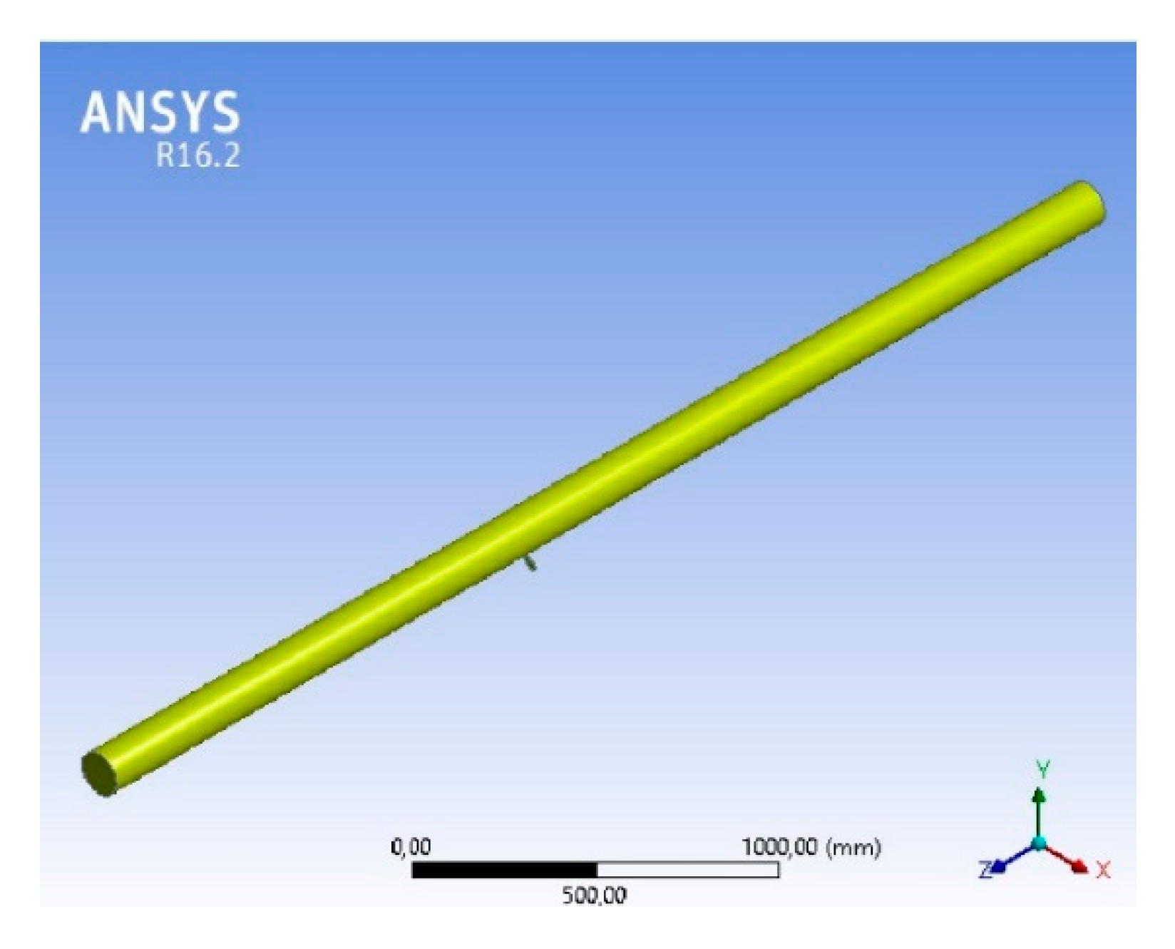
A 3D CFD model was implemented in the Ansys environment [30]. A geometric model, having the same features of the experimentally tested pipe, was generated with a rectangular transversal orifice. A prismatic rectangular protrusive element was then modelled, with a height equal to 5 times the equivalent diameter, D_eq, of the orifice, i.e., equal to 13.81 mm, useful to effectively fix the outlet boundary condition of the model, set constant and equal to atmospheric pressure. The fluid domain of interest was generated, removing smaller overlapping sub-domains, to correctly solve the flow physics (Figure 3).

The ANSYS software (ANSYS Italia s.r.l., Milan, Italy) was employed to solve steady three-dimensional (3D) Navier-Stokes equations. A realizable k-ε turbulence model was selected from among those manageable using the software, both for its reliability with fully developed flows and for its capability to assure effective results in limited computational times. A Semi-Implicit Method for Pressure Linked-Equation (SIMPLE) algorithm was employed for pressure-velocity coupling, for a faster convergence, with second order accuracy. A sensitivity analysis was performed to set the mesh resolution level, which was able to define the right balance between allowable results and computational efforts. Three mesh resolutions were tested, by varying the sizing and, thus, the number of elements, composing both the pipe and the fluid domain, as summarized in

Table 4. Size settings for the 3 considered mesh resolutions.

Resolution Level	Number of Elements	Element Size (mm)	Body Sizing (Pipe)		Body Sizing 2 (Fluid Domain)	Body Sizing 3 (Leak) (mm)
			Sphere Radius (mm)	Element Size (mm)	Element Size (mm)
Coarse	2,101,406	15	180	3	10	Not defined
Medium	9,031,221	10	180	2	5	Not defined
Fine	22,341,500	8	180	2	3	2

.

Medium resolution was chosen for simulations because, although the finer resolution provided better correlation between experimental and numerical data, it entailed significantly longer computational times, at the expense of relative improvement of experimental-numerical scatters. Indeed, relative scatters of mean velocity at the leak orifice in the order of 11.50% were observed with the medium resolution, against the 4.50% of the finer one (

Table 5. Scatters and computational time for considered mesh resolution levels.

Resolution Level	Experimental-Numerical Scatters (%)	Computational Time (h)
Coarse	20.81%	~12
Medium	11.45%	~24
Fine	4.48%	~36

).

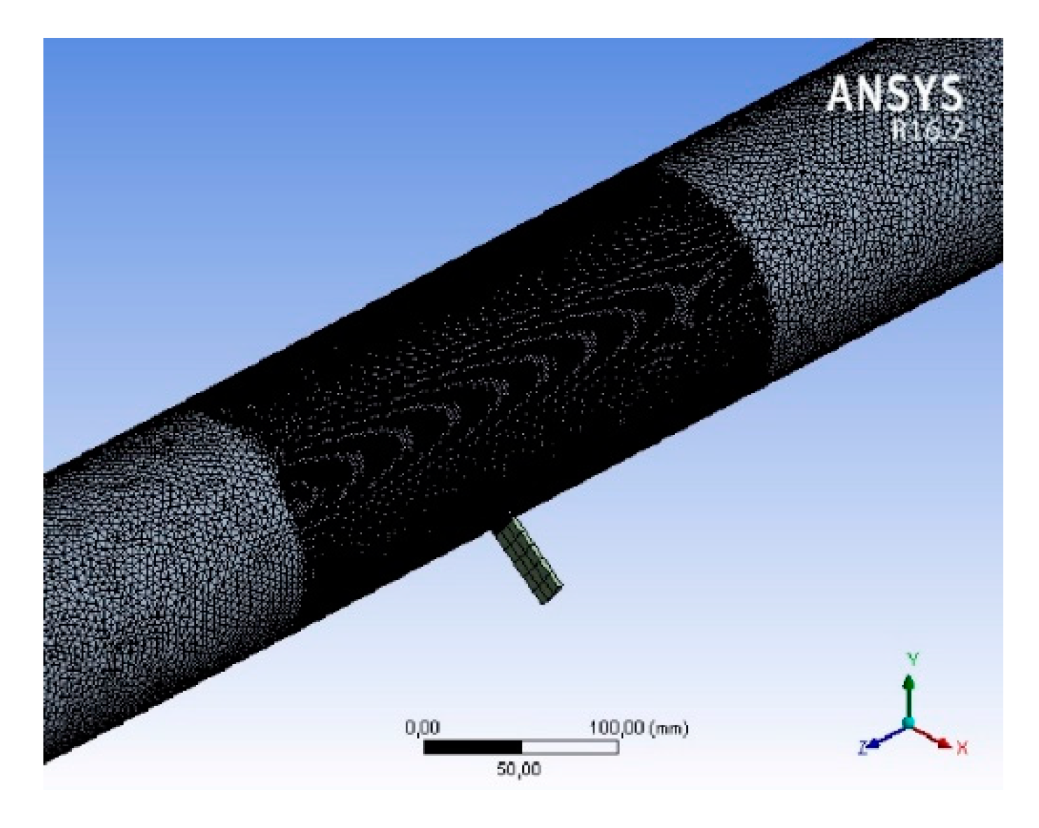
The chosen mesh was composed of 9 million tetrahedral elements with unitary sizing of 10 mm; however, to improve the accuracy of the calculation within the domain across the leak, a finer mesh was adopted in the neighbourhood of the rectangular orifice, setting a sphere of influence (with radius 180 mm) with the centre in the orifice barycentre. Tetrahedral geometry was applied to both the pipe and the fluid domain, whereas hexahedral elements were considered for the protrusive domain (Figure 4).

Since the leakage was modelled like a discharge flowing into atmosphere, the pressure at the leak was set to 0. Mass-flow rate and pressure were set as inlet boundary conditions using available experimental data, whereas the pressure at the outlet was analytically estimated using Hazen-William’s head-loss equation with the roughness coefficient set to 150. With reference to the transversal rectangular orifice, in order to match the performed laboratory experiments, 22 operating conditions with flow rate Q_in of 10, 20 and 30 L/s and pressure P varying from 1 to 7 bar were numerically simulated. Moreover, a further 47 simulations were performed with reference to different geometric configurations of the orifice, resulting in 69 different flow rate-pressure pairings overall.

As an example, the setting parameters with reference to inlet flow rate Q_in = 20 L/s and pressure P = 6.54 bar are reported in

Table 6. Setting boundary conditions at Q_in = 20 L/s and P = 6.54 bar.

Inlet Section			Outlet Section		Leak Section
Qin	Pin		Pout		Pl
(kg/s)	(Pa)	(bar)	(Pa)	(bar)	(Pa)
20.62	663′662	6.64	663′293	6.63	0

.

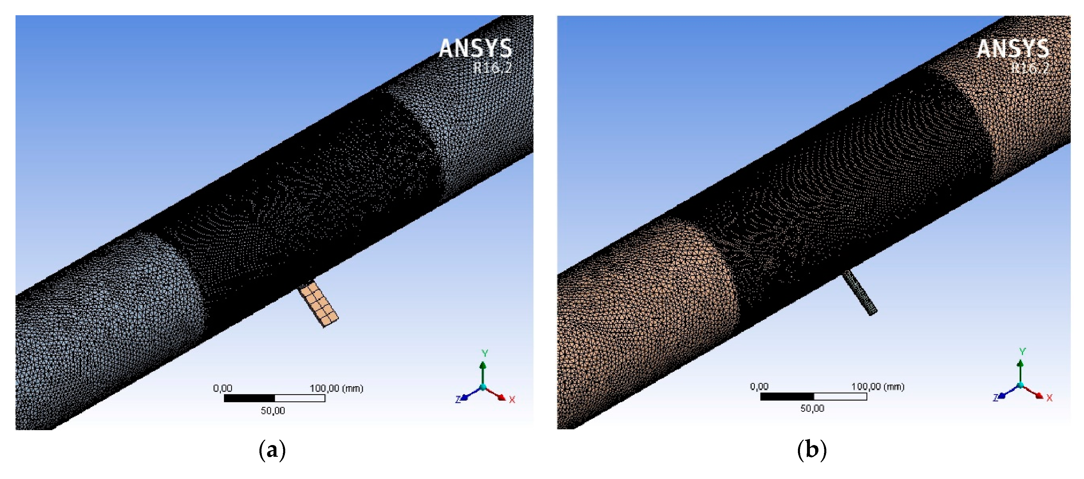
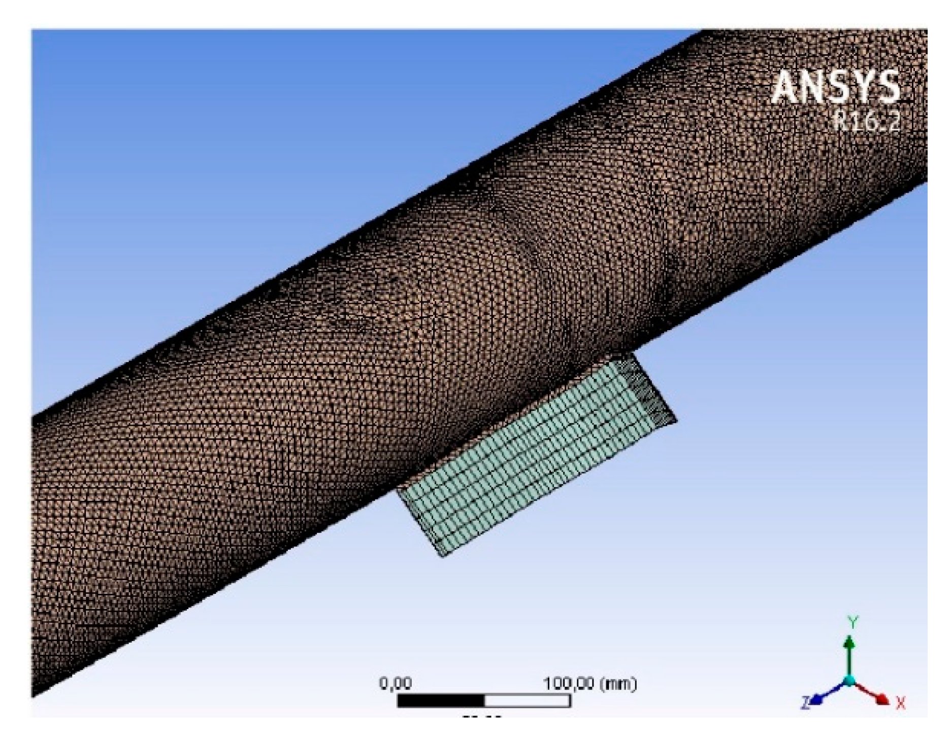
The designed geometrical configurations are shown in Figure 5 and Figure 6. In Figure 5a, the simulated orifice has the same area of the experimentally tested rectangular orifice (Figure 3) but a longitudinal orientation, whereas in Figure 5b, a circular orifice with the same area as the previous model was employed. Finally, a longitudinal crack (Figure 6) with a length of 200 mm and thickness of 1 mm was simulated, aimed at reproducing the geometrical configuration of a typical crack for a PVC-A pipe.

The leak flow rate Q_l and the averaged velocity V_l were thus estimated at the interface between the fluid domain and the prismatic rectangular protrusive element, by applying an area-weighted integrative approach.

3. Results and Discussion

From the experimental tests, the water loss Q_l for each value of pressure P performed was determined, as reported in

Table 7. Results of experimental static tests.

Qin = 10 L/s			Qin = 20 L/s			Qin = 30 L/s
TEST ID	P (bar)	Ql (L/s)	TEST ID	P (bar)	Ql (L/s)	TEST ID	P (bar)	Ql (L/s)
1	1.285	0.578	15	1.154	0.513	30	1.070	0.409
2	1.487	0.898	16	1.188	0.493	31	1.566	0.527
3	1.956	0.710	17	1.667	0.645	32	2.050	0.631
4	2.171	0.752	18	2.038	0.640	33	2.459	0.767
5	3.046	0.951	19	2.503	0.794	34	2.925	0.884
6	3.568	0.973	20	2.526	0.807	35	3.560	0.965
7	3.922	1.096	21	3.065	0.816	36	3.888	1.007
8	4.639	1.095	22	3.491	0.891	37	4.361	1.087
9	4.639	1.095	23	3.873	0.989	38	5.013	1.147
10	4.904	1.208	24	3.990	1.008	39	5.607	1.193
11	5.600	1.231	25	4.766	1.111	40	6.096	1.254
12	5.966	1.267	26	5.224	1.153	41	6.382	1.253
13	6.563	1.337	27	5.451	1.187	42	6.966	1.374
14	6.941	1.376	28	6.550	1.317
			29	7.214	1.400

.

Parameters of both the leakage law and the FAVAD approach were calibrated. Specifically, leakage coefficient C = 0.524 and leakage exponent N = 0.498 of Equation (2) were derived by minimizing the RMSE with Equation (8). They correspond to a Nash-Sutcliffe model efficiency coefficient (NSE) of 0.940, highlighting a significantly high accuracy. Moreover, C = 0.488 and N = 0.531 were defined by maximizing Equation (9) with NSE = 0.950.

The FAVAD exponent of Equation (3) υ = 0.587 was calibrated with Equation (8), corresponding to NSE = 0.939, whereas v = 0.579 was derived by maximizing the NSE to 0.950. For the sake of simplicity, parameters from the RMSE minimization were taken into account for the next assessments, since the values of NSE obtained by the two different approaches resulted in being significantly close to each other.

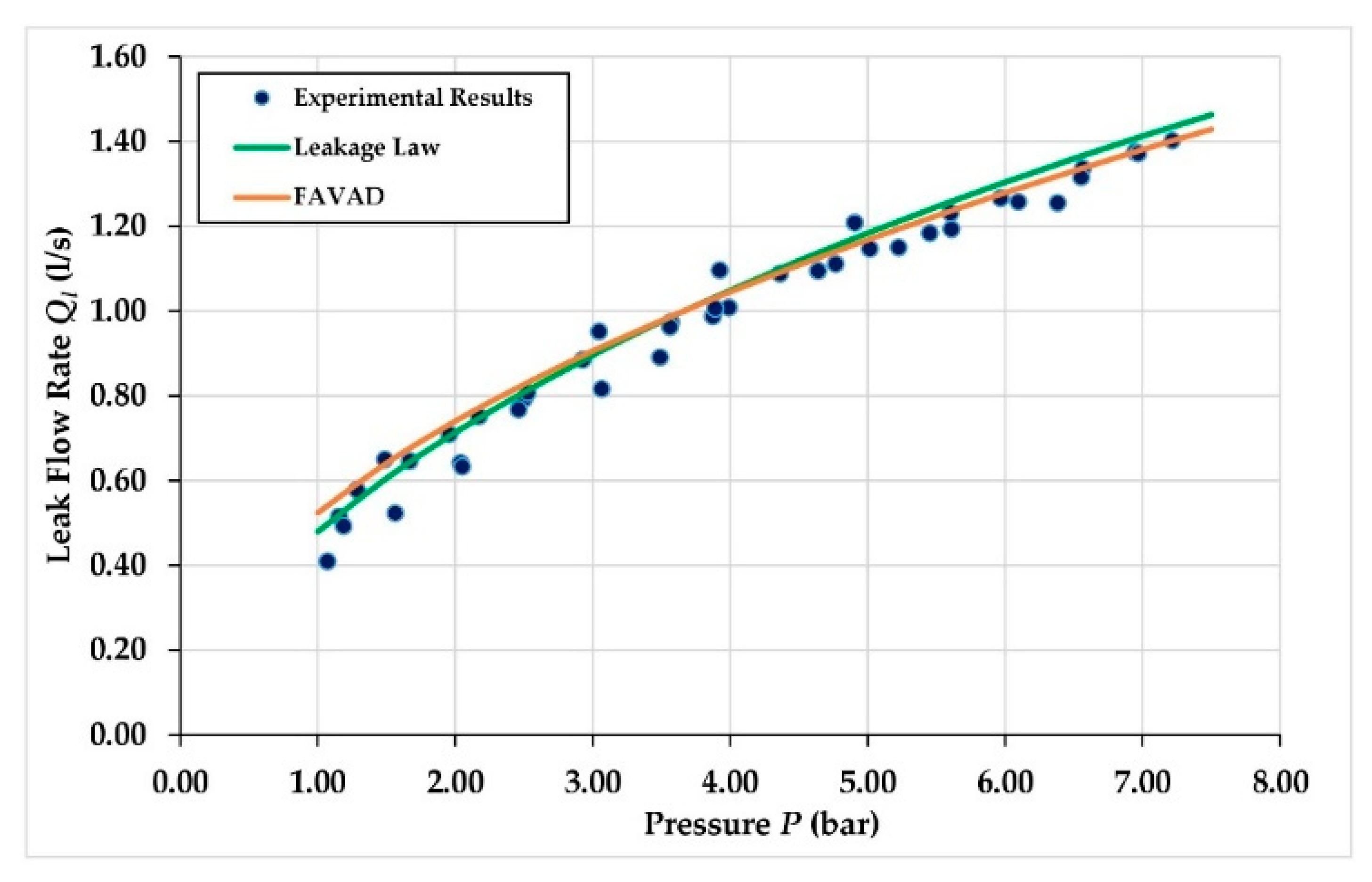
In Figure 7, the experimental results, compared with the derived theoretical equations, are plotted.

Both the Leakage Law (LL) and FAVAD equations presented significantly high correlation with the experimental data for pressure P higher than 2.50 bar, with relative scatter in the order of ±10%, corresponding to a p-value of 2.20 × 10⁻²⁰ for LL and 2.32 × 10⁻²⁰ for FAVAD at the significance level of 95%.

Specifically, for P ≥ 4 bar scatters not greater than ±5% were observed (p-value of 3.27 × 10⁻¹¹ for LL and 3.71 × 10⁻¹¹ for FAVAD). With reference to pressure P ≤ 2.50 bar, greater discrepancies were observed, instead, reaching scatters up to 32.5% with leakage law at Q_in = 30 L/s and P = 1.00 bar (p-value of 0.034 for both LL and FAVAD). Nevertheless, this dissimilarity corresponds to a simulated leak flow rate of 0.54 L/s, against the experimental value of 0.41 L/s. Thus, in absolute terms, it could be justified by the uncertainties related to the experimental observations, affecting most at lower pressure.

The experimental coefficient N obtained by the aforementioned calibration is significantly close to the theoretical value 0.50 of the leakage law. This result is explicable considering that the tested PVC-A pipe was completely new and did not experience any specific stress condition before. Moreover, neither visco-elastic behaviour nor further degradation effects were observed during the experiments, both the pipe and the orifice remaining of constant shape and size. This could be justified by the constant acting pressure during each test (always lower than the nominal pressure) and by the short test duration (300 s). Only slight flaws were observed around the orifice boundary, ascribable to the orifice drilling process.

Observed results for leakage exponent N were strictly in compliance with the study by Greyvenstein and van Zyl [12], hence, C increases proportionally to pipe wear.

The experimental and numerical results confirmed that the loss flow rate increases at pressure increasing. As shown in Table 6, the highest value of the leak flow rate was observed at the operating condition of P = 7 bar. However, the range of leak flow rate varied in a strict range, from 0.41 L/s to 1.40 L/s.

In

Table 8. Calibration of leakage law and FAVAD parameters with experimental and numerical analysis.

LL & FAVAD Parameters	Experimental Results	Numerical Results
	Transversal Orifice	Transversal Orifice	Longitudinal Orifice	Circular Orifice	Longitudinal Crack
C	0.524	0.635	0.657	0.614	1.606
N	0.498	0.454	0.498	0.523	0.522
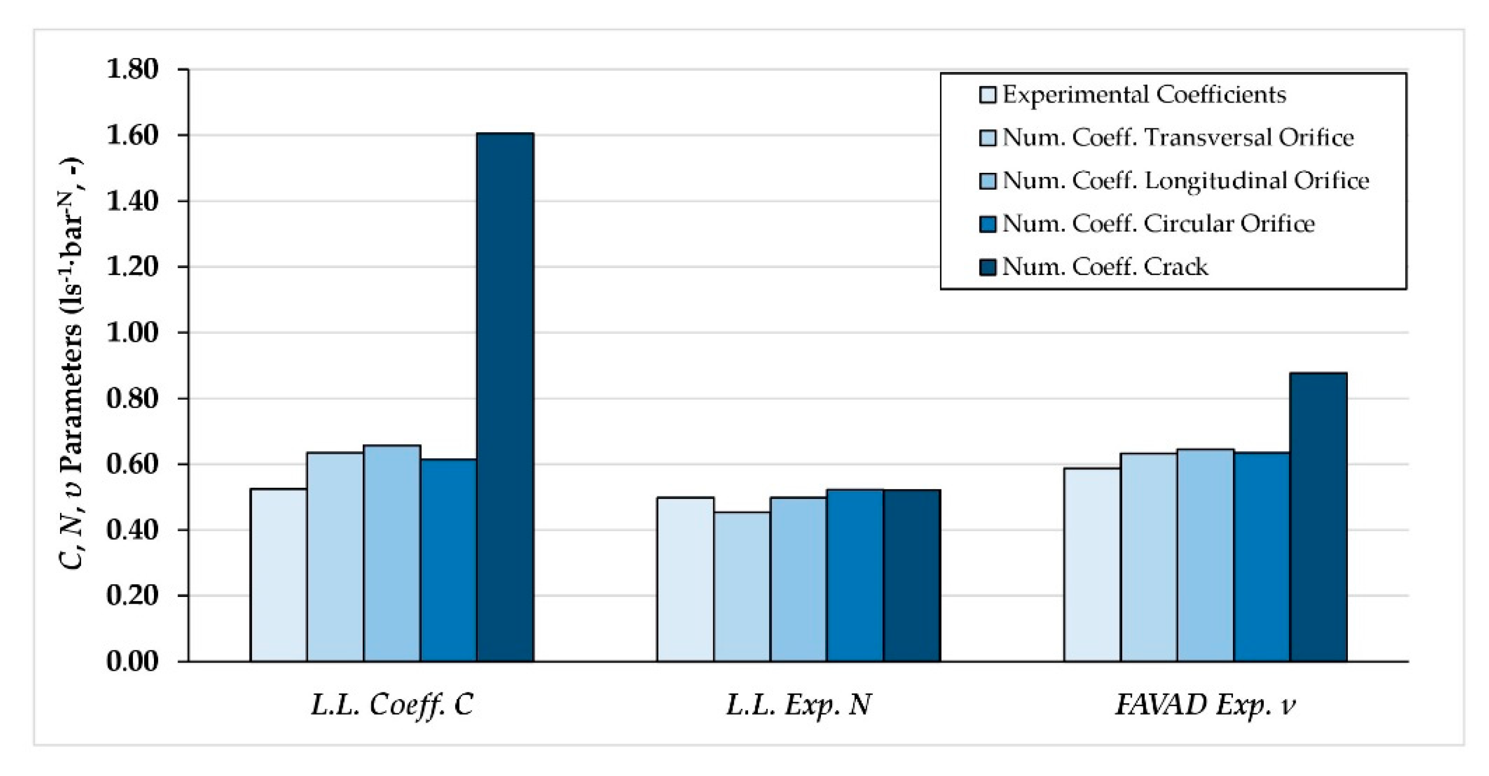
ν	0.587	0.632	0.645	0.635	0.877

and Figure 8, the results of calibration for the parameters of both Equation (2) and (3) from the CFD numerical simulations are summarized and compared with numerical results, with reference to the four types of considered orifices.

With reference to the transversal orifice, the numerical simulations provided the overestimation of the leakage coefficient C of 0.635 against the experimental value of 0.524. On the contrary, the leakage exponent was lower than the experimental one, however in the range observed by Greyvenstein and van Zyl [12] for circumferential cracks of PVC-U pipes. From the experimental-numerical comparison, relative scatters up to ±20% were observed for P ≤ 2.50 bar, whereas scatters in the order of 10÷15% were defined for higher pressure values.

Simulations of the longitudinal orifice provided both a C and N coefficient higher than the simulated transversal type. Specifically, the leakage exponent N was equal to the experimental value, at the same time, resulting very close to the theoretical value of 0.50. The circular orifice gave a lower leakage coefficient C than previous cases, whereas the leakage exponent N was higher, in any case comparable to both the experimental and the theoretical value.

Simulations of a longitudinal crack returned a C coefficient significantly higher (C = 1.61). This was due to the greater overall area of the orifice. The exponent N of the leakage law was, also in this case, in agreement with both the experimental value and further numerical simulations, thus, being contrary with Greyvenstein and van Zyl [12], who observed N values between 1.38 and 1.85 for PVC-U pipes, instead.

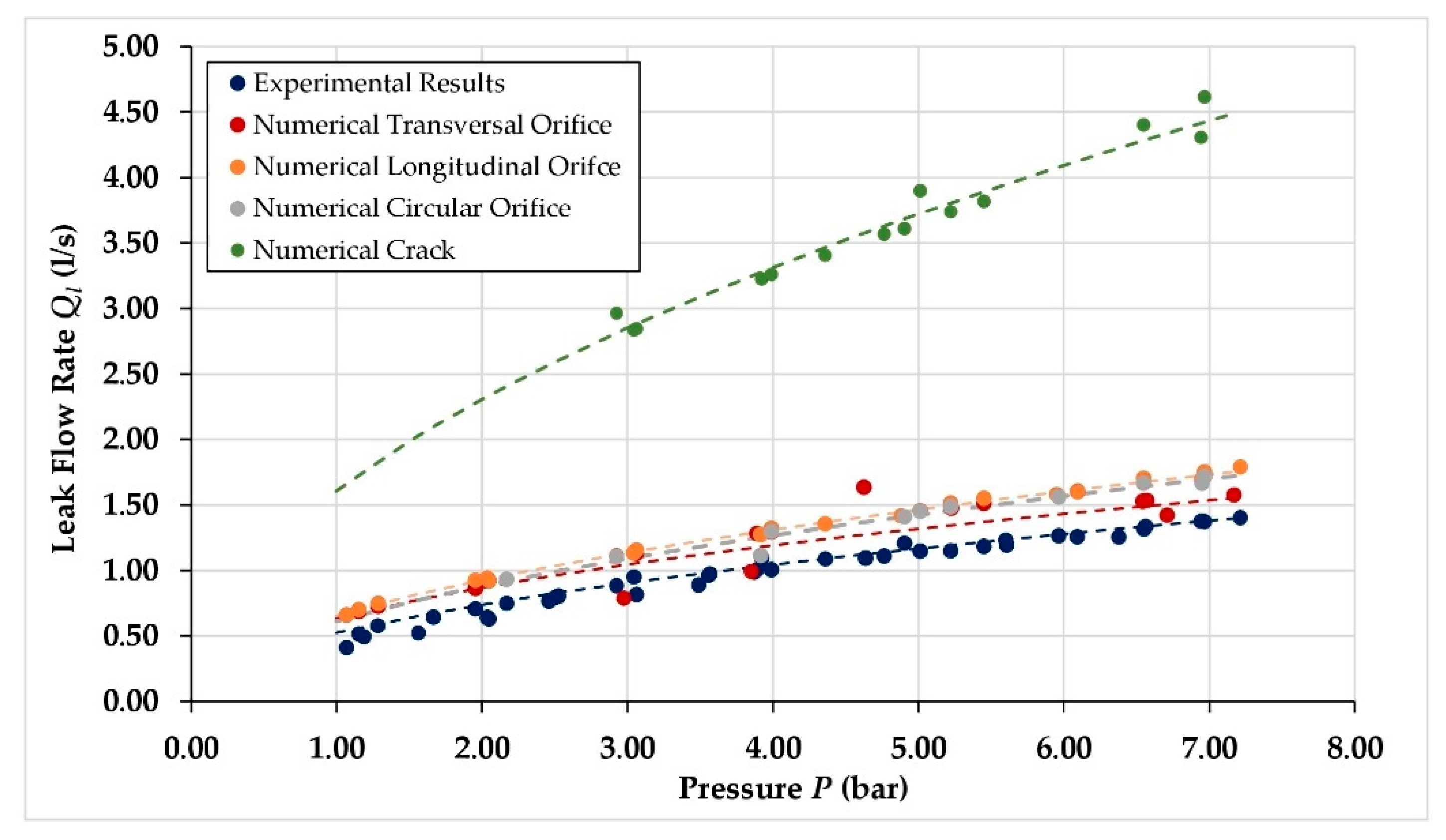
In Figure 9, a comparison between the experimental and numerical results (pointer) and the related leakage law application (dashed line) is plotted. The strict correlation between the results for the longitudinal and circular orifice is observed, resulting in slightly higher results than for the transversal orifice, showing a secondary influence of the orifice shape and orientation in the leak flow rate assessment. Nevertheless, the simulated transversal orifice overestimated the experimental results in terms of leak flow rate. This scatter can be however justified by the order of magnitude of the investigated leak flow rate (in the order of 1 L/s), which can be significantly affected by uncertainties of the recording and processing analysis of the experiments; furthermore, the orifice on the tested pipe did not present a completely regular rectangular shaped form.

The FAVAD exponent υ, with reference to the transversal orifice, overestimated the experimental value, defining scatters between 10% and 15% for P ≤ 2.50 bar and up to 21% for higher p-values. However, it was pretty comparable for numerical simulations of transversal, longitudinal and circular orifices, being in the order of 0.63–0.64. For the longitudinal crack, a higher υ exponent was observed, being close to 0.88, instead.

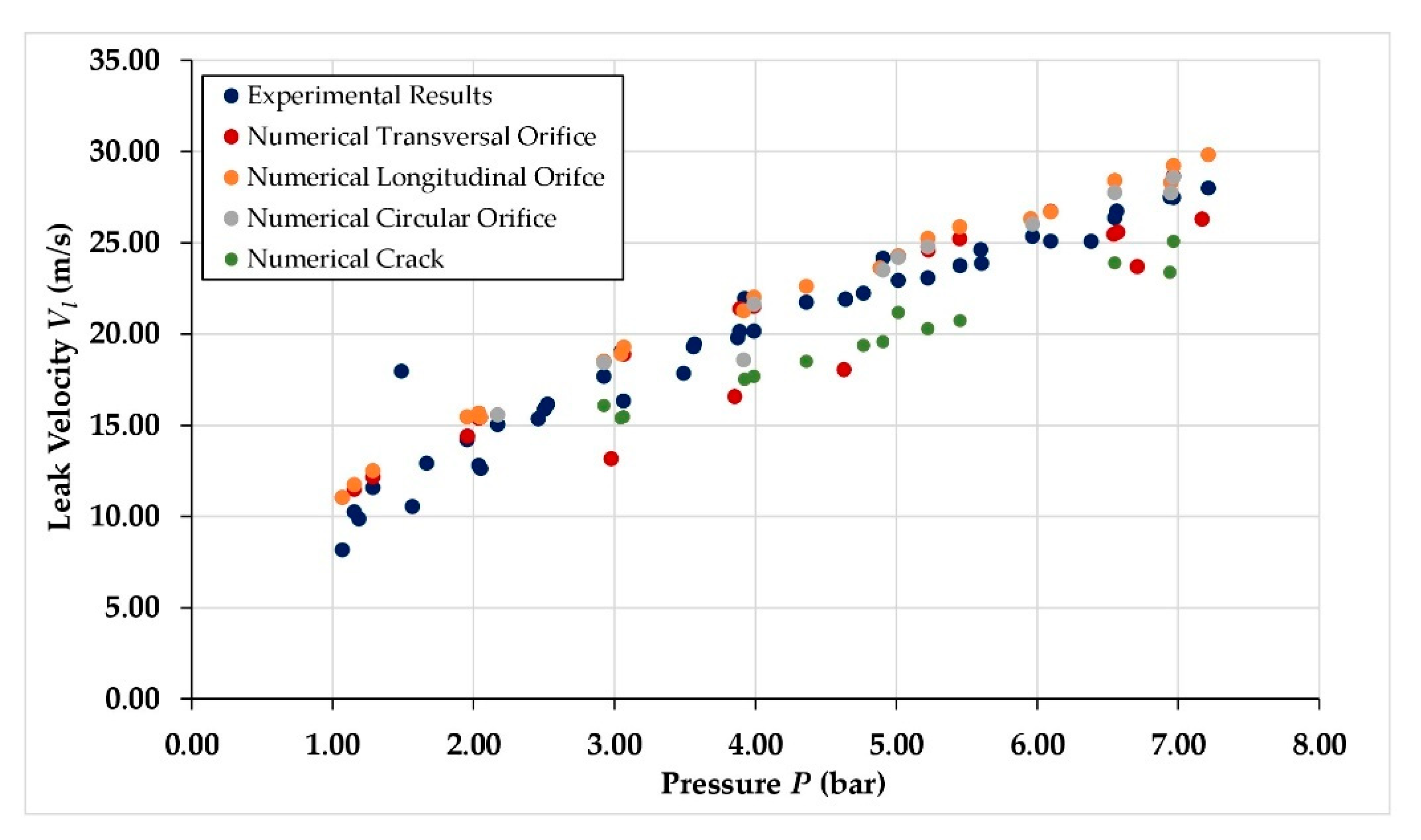
In terms of mean velocity at the leak, from the comparison between the experimental and numerical results for the transversal orifice, an overestimation of the numerical simulation of 10% was observed at P < 2 bar, whereas discrepancies not higher than ±5% resulted for higher P.

By comparing the numerical results of further orifice geometries, it was observed that comparable values were achieved by both the transversal and longitudinal orifice and the circular one, whereas slightly lower velocity was defined for the longitudinal crack (Figure 10).

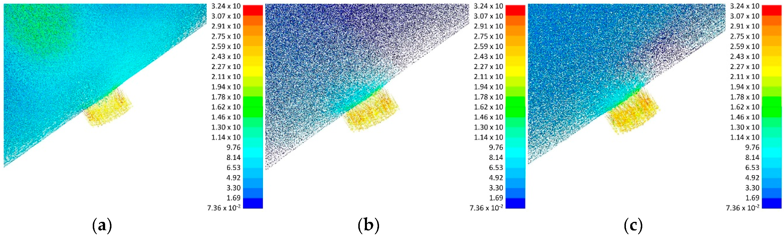
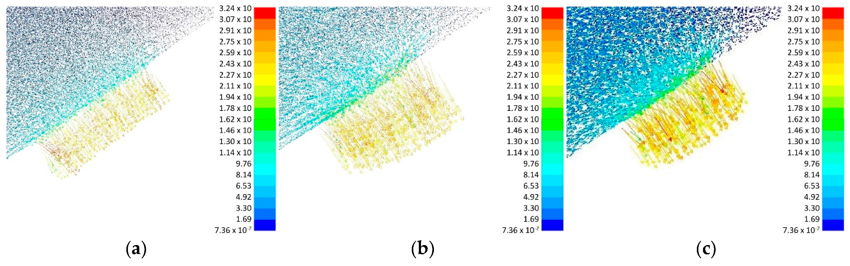
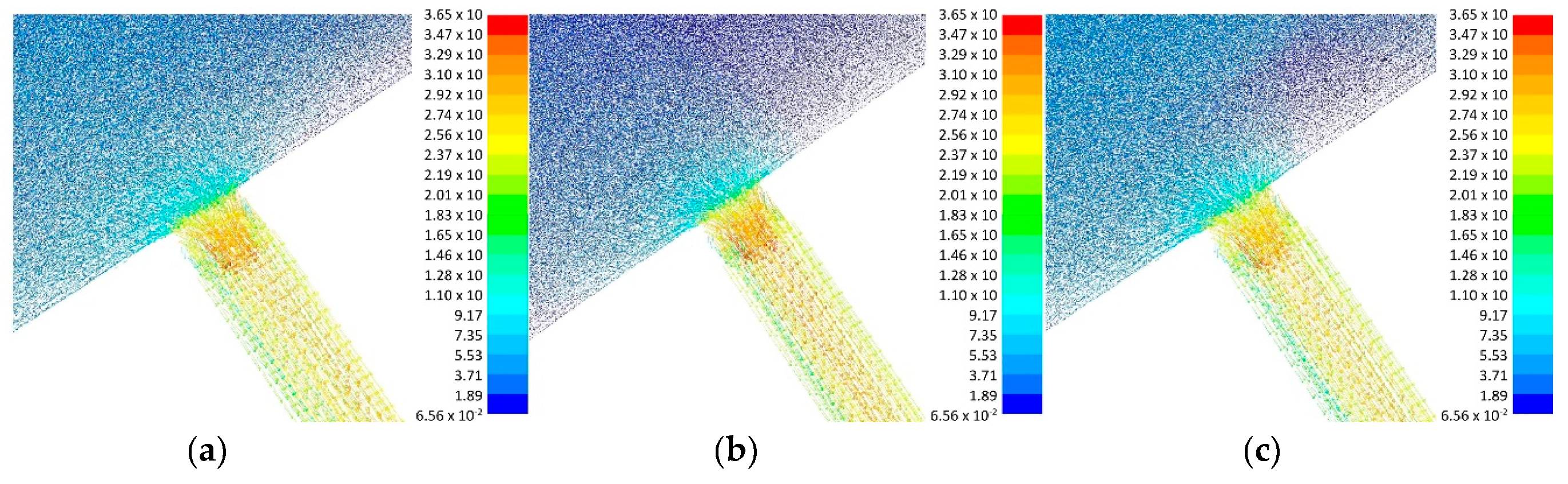
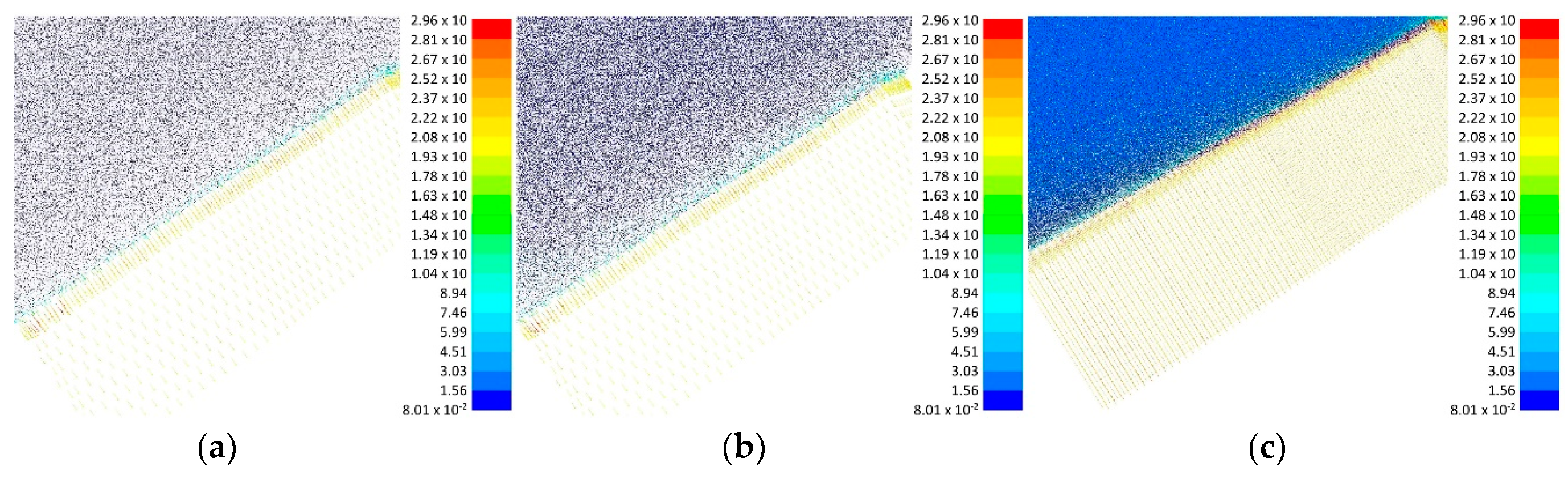
This is observable in Figure 11, Figure 12, Figure 13 and Figure 14 where the velocity fields in the region around the orifice are plotted for each simulated geometry at Q_in = 10, 20 and 30 L/s and P = 5 bar. Strictly comparable velocity fields for the transversal, longitudinal and circular orifice are detected for the whole range of investigated flow rates. However, slightly lower velocities occur at the longitudinal crack because of the greater efflux along the crack.

4. Conclusive Remarks

The significant leakage-related water losses affecting pressurized water systems calls for the definition of specific methodologies for estimating the leak discharge-head relation. With reference to the innovative PVC-A material, the hydraulic behaviour of which under different operative conditions is still unexplored, an experimental and numerical investigation was conducted. Both the general expression of the leakage law and the FAVAD equation resulted in being reliable for forecasting the water dispersed by orifices with different geometry and orientation, in the range of pressure typically experienced in water supply and distribution systems. According to the experimental results for a transversal rectangular orifice, discharge coefficient C and discharge exponent N of leakage law were found to equal 0.635 and 0.498, respectively, whereas FAVAD exponent $\nu$ = 0.657 was observed. From both the experimental and numerical approaches, the leakage exponent N was observed to be consistent with the theoretical value of 0.50. In addition, the longitudinal orientation of the leak relative to the pipe axis was observed to play a minor role on the magnitude of the leak flow rate, generating on average 7.2% higher leakage at the same pressure.

Concerning the simulated longitudinal crack, owing to the larger orifice extension, a significant increase of loss in flow rate was observed. On the other hand, the calculated mean velocity at the leak was lower than the rectangular and circular ones. This could be due to the longer extension of the orifice, defining a progressive reduction of flow rate across the area from upstream to downstream sections.

The performed experimental analysis was based on static tests, with constant pressure and short stress duration. Experimental and numerical assessment of PVC-A pipes under dynamic operations of the system, aiming at reproducing the daily pattern of a WDN, are needed to gain a full understanding of the leakage behaviour of PVC-A pipes. Specific focus on the visco-elastic behaviour of this material under variable and higher system pressures than those considered in this study is required for its hydraulic characterization. Moreover, updating the laboratory set-up could allow the investigation to be extended to pressure operations higher than those investigated so far.

This research is expected to aid in the assessment of the interaction between head and leak flow in innovative materials for pressurized hydraulic systems, providing evidence of experimental results with results from CFD numerical simulations.

References

- Lambert, A. Accounting for losses: The bursts and background concept. Water Environ. J. 1994, 8, 205–214. [Google Scholar] [CrossRef]
- De Paola, F.; Galdiero, E.; Giugni, M. A jazz-based approach for optimal setting of pressure reducing valves in water distribution networks. Eng. Optim. 2016, 48, 727–739. [Google Scholar] [CrossRef] [Green Version]
- Pugliese, F.; De Paola, F.; Fontana, N.; Giugni, M.; Marini, G. Performance of vertical-axis pumps as turbines. J. Hydraul. Res. 2018, 56, 482–493. [Google Scholar] [CrossRef]
- Morani, M.C.; Carravetta, A.; Fecarotta, O.; McNabola, A. Energy transfer from the freshwater to the wastewater network using a PAT-equipped turbopump. Water (Switzerland) 2020, 12, 38. [Google Scholar] [CrossRef] [Green Version]
- Lambert, A. What do we know about pressure: Leakage relationships in distribution systems? In Proceedings of the IWA Conference System Approach to Leakage Control and Water Distribution Systems Management, Brno, Czech Republic, 16–18 May 2001. [Google Scholar]
- Ferrante, M.; Massari, C.; Brunone, B.; Meniconi, S. Leak behaviour in pressurized PVC pipes. Water Sci. Technol. Water Supply 2013, 13, 987–992. [Google Scholar] [CrossRef]
- Managing Leakage by Managing Pressure: A Practical Approach. Available online: http://aquageo.es/wp-content/uploads/2012/10/MANAGING-LEAKAGE-BY-MANAGING-PRESSURE.pdf (accessed on 23 June 2020).
- Walski, T.; Bezts, W.; Posluszny, E.T.; Weir, M.; Whitman, B.E. Modeling leakage reduction through pressure control. J. Am. Water Work. Assoc. 2006, 98, 147–155. [Google Scholar] [CrossRef]
- May, J. Pressure dependent leakage. In World Water and Environmental Engineering; WEF Publishing Inc.: London, UK, 1994. [Google Scholar]
- Farley, M.; Trow, S. Losses in Water Distribution Networks; Control; IWA Publishing: London, UK, 2003; ISBN 9781900222112. [Google Scholar]
- Van Zyl, J.E.; Clayton, C.R.I. The effect of pressure on leakage in water distribution systems. Proc. Inst. Civ. Eng. Water Manag. 2007, 160, 109–114. [Google Scholar] [CrossRef]
- Greyvenstein, B.; van Zyl, J.E. An experimental investigation into the pressure—Leakage relationship of some failed water pipes. J. Water Supply Res. Technol. AQUA 2007, 56, 117–124. [Google Scholar] [CrossRef]
- Cassa, A.M.; van Zyl, J.E.; Laubscher, R.F. A numerical investigation into the effect of pressure on holes and cracks in water supply pipes. Urban Water J. 2010, 7, 109–120. [Google Scholar] [CrossRef]
- De Paola, F.; Giugni, M. Leakages and pressure relation: An experimental research. Drink. Water Eng. Sci. 2012, 5, 59–65. [Google Scholar] [CrossRef] [Green Version]
- Ferrante, M.; Massari, C.; Todini, E.; Brunone, B.; Meniconi, S. Experimental investigation of leak hydraulics. J. Hydroinform. 2013, 15, 666–675. [Google Scholar] [CrossRef]
- Franchini, M.; Lanza, L. Use of Torricelli’s equation for describing leakages in pipes of different elastic materials, diameters and orifice shape and dimensions. Proc. Eng. 2014, 89, 290–297. [Google Scholar] [CrossRef] [Green Version]
- Ferrante, M.; Massari, C.; Brunone, B.; Meniconi, S. Experimental evidence of hysteresis in the head-discharge relationship for a leak in a polyethylene pipe. J. Hydraul. Eng. 2011, 137, 775–780. [Google Scholar] [CrossRef]
- Massari, C.; Ferrante, M.; Brunone, B.; Meniconi, S. Is the leak head-discharge relationship in polyethylene pipes a bijective function? J. Hydraul. Res. 2012, 50, 409–417. [Google Scholar] [CrossRef]
- Ferrante, M. Experimental investigation of the effects of pipe material on the leak head-discharge relationship. J. Hydraul. Eng. 2012, 138, 736–743. [Google Scholar] [CrossRef]
- De Paola, F.; Galdiero, E.; Giugni, M.; Papa, R.; Urciuoli, G. Experimental investigation on a buried leaking pipe. Proc. Eng. 2014, 89, 298–303. [Google Scholar] [CrossRef] [Green Version]
- Lambert, A.; Hirner, W. Losses from Water Supply Systems: Standard Terminology and Recommended Performance Measures; IWA Blue Pages; IWA Publishing: London, UK, 2000. [Google Scholar]
- Alegre, H.; Baptista, J.M.; Cabrera, E.; Cubillo, F.; Duarte, P.; Hirner, W.; Merkel, W.; Parena, R. Performance Indicators for Water Supply Services, 3rd ed.; Water Intelligence Online; IWA Publishing: London, UK, 2016. [Google Scholar] [CrossRef]
- Managing Leakage by District Metered Areas: A Practical Approach. Available online: http://www.geocities.ws/kikory2004/39_Water21_5th_article_DMA.pdf (accessed on 23 June 2020).
- EPA. Water Audits and Water Loss Control for Public Water Systems. Available online: https://www.epa.gov/sites/production/files/2015-04/documents/epa816f13002.pdf (accessed on 23 June 2020).
- Cassa, A.M.; van Zyl, J.E. Predicting the head-leakage slope of cracks in pipes subject to elastic deformations. J. Water Supply Res. Technol. AQUA 2013, 62, 214–223. [Google Scholar] [CrossRef]
- Shehadeh, M.; Shahata, A.I. Modelling the effect of incompressible leakage patterns on rupture area in pipeline. CFD Lett. 2013, 5, 132–142. [Google Scholar]
- Danesh, M.; Hassan, A. Estimation of discharge coefficient in orifice meter by CFD simulation. In Proceedings of the 2018 International Conference on Pure and Applied Science, Koya University, Koysinjaq, Iraq, 23–24 April 2018. [Google Scholar]
- Shah, M.S.; Joshi, J.B.; Kalsi, A.S.; Prasad, C.S.R.; Shukla, D.S. Analysis of flow through an orifice meter: CFD simulation. Chem. Eng. Sci. 2012, 71, 300–309. [Google Scholar] [CrossRef]
- Scott, D.V. Advanced Materials for Water Handling: Composites and Thermoplastics, 1st ed.; Elsevier: Amsterdam, The Netherlands, 2000; ISBN 9781856173506. [Google Scholar]
- ANSYS Inc. Fluent, a ANSYS Fluent 12.0 User’s Guide. Available online: https://www.afs.enea.it/project/neptunius/docs/fluent/html/ug/main_pre.htm (accessed on 23 June 2020).
Figure 1.
Graphic scheme of investigated PVC-A pipe with transversal orifice.
Figure 2.
Layout of the experimental setup at the Laboratory of Hydraulics (University of Naples Federico II).
Figure 3.
Geometric model of the PVC-A with transversal orifice implemented in Ansys environment.
Figure 4.
Tetrahedral mesh of the fluid domain for transversal orifice in Ansys environment.
Figure 5.
Computational Fluid Dynamics (CFD) modelling of a (a) rectangular orifice with longitudinal orientation and (b) circular orifice in Ansys environment.
Figure 6.
CFD modelling of a longitudinal crack in Ansys environment.
Figure 7.
Comparison between experimental results and leakage law and FAVAD models.
Figure 8.
Comparison between experimental and numerical calibration of leakage law and FAVAD parameters.
Figure 9.
Comparison between experimental and numerical results.
Figure 10.
Leak velocity comparison between experimental data and numerical simulations.
Figure 11.
Velocity field for transversal orifice at P = 5.0 bar and Qin = (a) 10 L/s, (b) 20 L/s, (c) 30 L/s.
Figure 12.
Velocity field for longitudinal orifice at P = 5.0 bar and Qin = (a) 10 L/s, (b) 20 L/s, (c) 30 L/s.
Figure 13.
Velocity field for circular orifice at P = 5.0 bar and Qin = (a) 10 L/s, (b) 20 L/s, (c) 30 L/s.
Figure 14.
Velocity field for longitudinal crack at P = 5.0 bar and Qin = (a) 10 L/s, (b) 20 L/s, (c) 30 L/s.