Discharge Estimation Using Tsallis and Shannon Entropy Theory in Natural Channels


1
Department of Hydrology, Indian Institute of Technology Roorkee, Roorkee 247667, India
2
Research institute for Geo-hydrological protection, National Research Council, via della Madonna Alta 126, 06128 Perugia, Italy
*
Author to whom correspondence should be addressed.
Water 2020, 12(6), 1786; https://doi.org/10.3390/w12061786
Submission received: 24 April 2020
/
Revised: 15 June 2020
/
Accepted: 20 June 2020
/
Published: 23 June 2020
(This article belongs to the Special Issue Fluvial Hydraulics and Applications)
Abstract
:Streamflow measurements during high floods is a challenge for which the World Meteorological Organization fosters the development of innovative technologies for achieving an accurate estimation of the discharge. The use of non-contact sensors for monitoring surface flow velocities is of interest to turn these observed values into a cross-sectional mean flow velocity, and subsequently, into discharge if bathymetry is given. In this context, several techniques are available for the estimation of mean flow velocity, starting from observed surface velocities. Among them, the entropy-based methodology for river discharge assessment is often applied by leveraging the theoretical entropic principles of Shannon and Tsallis, both of which link the maximum flow velocity measured at a vertical of the flow area, named the y-axis, and the cross-sectional mean flow velocity at a river site. This study investigates the performance of the two different entropic approaches in estimating the mean flow velocity, starting from the maximum surface flow velocity sampled at the y-axis. A velocity dataset consisting of 70 events of measurements collected at two gauged stations with different geometric and hydraulic characteristics on the Po and Tiber Rivers in Italy was used for the analysis. The comparative evaluation of the velocity distribution observed at the y-axis of all 70 events of measurement was closely reproduced using both the Shannon and Tsallis entropy approaches. Accurate values in terms of the cross-sectional mean flow velocity and discharge were obtained with average errors not exceeding 10%, demonstrating that the Shannon and Tsallis entropy concepts were equally efficient for discharge estimation in any flow conditions.
Keywords:
entropy; mean velocity; maximum velocity; discharge; rating curve; surface velocity; dip; secondary current; POME1. Introduction:
In open-channel hydraulics, the cross-sectional mean flow velocity is defined as the ratio of discharge Q to the area A of the flow. The cross-sectional mean flow velocity can be estimated in several ways. Conventionally, it is estimated using the velocity–area method, which is still followed in many countries [1]. This method has certain disadvantages, such as limited accuracy, and in some stations, its use may not be safe for the observer, especially during velocity observations of high flood conditions. Furthermore, the field practices of the area–velocity method is a time-consuming process. The most common instrument used for velocity measurement is the current meter, which is employed either from cableways or from bridges across the river, and the propeller vane of the current meter is placed at the desired depth level of a vertical to measure the point velocity. However, the use of a current meter is hampered during high flood conditions due to the difficulty in sampling point velocities in the lower part of the cross-sectional flow area.
An acoustic Doppler current profilers (ADCP) can also be used for the velocity measurement during high flow conditions, though many limitations exist. Furthermore, high flow conditions characterized by high turbulence may affect flow depth conditions due to rolling and pitching motions of the boat [2]. To overcome these difficulties, non-contact measurement techniques have been developed that use equipment, such as large-scale particle image velocimetry (LSPIV) [3,4] and surface velocity radar (SVR) [5,6]. However, these non-contact techniques also have some limitations: the radar technology may be affected during low flow when the backscatter of the beam can be swamped by high noise, while the LSPIV might not be suitable for measurements during scarce seeding, illumination conditions, and/or overnight floods [7]. Even so, the use of both SVR and LSPIV is suitable for monitoring high flows by overcoming the limitations of conventional contact-based techniques, as well as avoiding the unsafe conditions faced by the operators during high flows.
Chiu [8,9,10] introduced the application of Shannon entropy theory [11] in hydraulic engineering by linking the probability distribution of the velocity and the physical space in terms of curvilinear coordinates. Using this entropy theory, the cross-sectional mean velocity is estimated by sampling the maximum flow velocity occurring at a flow depth vertical called the y-axis and linking it with the cross-sectional mean flow velocity, which is subsequently used for estimating the flow discharge. Chiu estimated the velocity distribution equation based on the principle of maximum entropy (POME) [12] and established a linear relationship between the cross-sectional mean flow velocity and the maximum flow velocity using an entropic parameter Ω(M) [13]. Later on, Moramarco’s [14] work based on Chiu’s approach expressed the simplified form of the entropy-based velocity distribution equation, where by starting from the measure of the maximum velocity and knowing the bathymetry, the 2D velocity distribution can be established. The maximum flow velocity generally occurs at the water’s surface; however, due to the presence of secondary currents [15], it may occur below the water’s surface, which is known as the dip-phenomenon linked to the concept of aspect ratio and it is a characteristic of both narrow and wide channels [16,17]. The maximum flow velocity can be easily sampled using any measuring instrument, such as a current meter, ADCP, LSPIV, and SVR. However, the non-contact discharge estimation concept is based on the estimation of the maximum flow velocity, which is inferred by measuring the surface flow velocity across the river site using, e.g., LSPIV or SVR techniques [18,19], and applying Shannon’s entropy-based approach, such as that proposed by, e.g., Chiu [8] or Moramarco [14].
Tsallis entropy is a special case of Shannon entropy [20]. Singh [21] introduced the Tsallis entropy concept in hydraulic engineering by presenting the one-dimensional velocity distribution equation, as well as the two-dimensional velocity distribution, and found that the Tsallis entropy-based concept is either superior or comparable with the Shannon entropy-based concept [22,23,24]. However, from a practical point of view, it would be interesting to explore the performance of the two different entropy-based approaches by leveraging only the velocity observations at the y-axis, for which many SVR pieces of equipment are employed for monitoring the discharge. In this context, this study aimed to present a comparison between Tsallis’ entropy-based approach and that of Shannon’s entropy for discharge estimation at river stations with different geometric and hydraulic characteristics. Unlike other studies [14,19], the analysis undertaken in this study to estimate the discharge only addresses the measurement of the maximum surface flow velocity at the y-axis and the observed dip.
Velocity datasets collected at the Pontelagoscuro station (Po River) and Ponte Nuovo station (Tiber River), both in Italy, were considered for the analysis. This paper is organized as follows: Section 2 provides the theoretical background of the non-contact discharge estimation using both Shannon and Tsallis entropies. Section 3 describes the details of the river gauge stations in this study. Section 4 describes the results achieved using these approaches and the comparative evaluation of flows estimated using both methods. Lastly, Section 5 presents the conclusion of the study.
2. Method
2.1. Tsallis Entropy-Based Non-Contact Discharge Estimation.
Singh [21] expressed the velocity distribution equation based on Tsallis entropy theory as:
where U is the point velocity in the longitudinal direction, is the maximum velocity of the channel section, G is the entropic parameter, h is the dip (depth of below the water’s surface), D is the depth of the flow, and y is the distance of the measuring point from the bottom of the channel. In the above equation, the y-axis is selected in such a way that it passes through the point of maximum velocity that generally occurs at the deepest vertical. However, the location of the y-axis can be identified using the historical record of streamflow measurements at channel sections. The entropic parameter (G) is characteristic of the channel section and it can be easily estimated through the pairs of cross-sectional mean flow and maximum velocity using a linear entropic relationship. The relation between the mean and maximum velocities based on Tsallis entropy follows a linear distribution, which is expressed as [21,23]:
where is the cross-sectional mean flow velocity and occurs at the deepest vertical flow depth of the flow section. Ω(G) is the state equilibrium constant (dimensionless parameter). The maximum flow velocity can be estimated using the surface flow velocity through Equation (1) based on Tsallis entropy as follows:
where is the surface flow velocity for the y-axis and h is the location of the maximum velocity below the free surface of the water. If h = 0, then This approach requires the identification of the deepest vertical established at the cross-section of interest and all velocity measurement points, i.e., the surface water velocity and velocity at different points on this vertical must be collected. Additionally, it requires that the ratio of the mean flow velocity to the maximum velocity is unique for the cross-section of interest.
2.2. Shannon Entropy-Based Non-Contact Discharge Estimation
Fulton [18] gave the non-contact discharge concept and developed a relationship between the surface flow velocity and the maximum flow velocity based on Shannon entropy theory. The Shannon entropy-based velocity distribution was derived by Chiu [8,9,10] and simplified by Moramarco [14]. It is expressed as:
where U is the longitudinal point velocity at any location on the y-axis; is the maximum flow velocity; M is Shannon’s entropy parameter, which is a property of a section [14]; D is the depth of flow; and y is the location of the velocity measuring point measured from the bottom of the channel.
The entropy parameter or constant M can be estimated using Equation (5):
The maximum flow velocity of a given vertical line can be estimated using Equation (6) by starting from the surface flow velocity measured at the same vertical and using Shannon entropy theory, as follows:
2.3. Cross-Sectional Mean Flow Velocity and Discharge Estimation
To compute the cross-sectional mean flow velocity and the corresponding discharge passing through the flow section using a non-contact technique based on the Tsallis and Shannon entropy concepts, the following step-by-step procedure was used:
- Identify the location of the y-axis (vertical where the maxum velocity is recorded) through historical records.
- Measure multiple point velocities along this vertical, including the surface water velocity on this identified y-axis.
- Tabulate the pairs of cross-sectional mean and maximum velocities for different flood events.
- Estimate Tsallis’ G value using Equation (2) and Shannon’s M value using Equation (5).
- Estimate the maximum velocity from the surface flow velocity measurements using Equation (3) for Tsallis’ theory and Equation (6) for Shannon’s theory, and compare these with the observed maximum velocity of that event.
- Estimate the cross-sectional mean velocity using Equation (2) for Tsallis’ theory and Equation (5) for Shannon’s theory.
- Determine the cross-sectional flow area corresponding to the recorded water surface level.
- Estimate the discharge using the estimated cross-sectional mean velocity obtained in step (8) and the cross-sectional area using Q = AV.
3. Study Area
To demonstrate the acceptability of the proposed flow estimation approach at a gauge station, two gauge sections, one each for the Po and Tiber Rivers in Italy, were considered. Flow data from the Ponte Nuovo station of the Tiber river (Italy) and Pontelagoscuro station of the Po river (Italy) were used to test the acceptability of the proposed non-contact discharge estimation based on the Tsallis entropy theory. The data sets consisted of multipoint velocity measurements made at a vertical of the flow section of an event using the current meter from the cableway. The number of velocity points sampled along the verticals was sufficient (more than ten for some verticals) to reconstruct the vertical velocity profiles and to identify the dip, even in the presence of secondary currents. Table 1 presents the details of such measurements made at the two stations at the Po and Tiber Rivers.
4. Results and Discussion
4.1. Non-Contact Discharge Assessment Using Tsallis Entropy
To evaluate the above-discussed procedure for discharge estimation using the Tsallis entropy theory, a total of 48 events of the Po River (from 1984 to 1992) and 22 events of the Tiber River (1985–2000) were considered. The velocity dataset was provided by the Agenzia Interregionale per il Fiume Po for the Po River and the Department of Environment, Planning, and Infrastructure of the Umbria Region for the Tiber River. For each of the selected measurements, the data refer to the (1) velocity points sampled along verticals in terms of the elevation above the bed and the corresponding measured value, (2) location of the vertical from the left sidewall, (3) hydrometric level, (4) mean flow velocity, and (5) discharge. For each event, was computed by starting from the surface velocity and the dip observed at the y-axis and using Equations (3) and (6) for Tsallis and Shannon entropy, respectively.
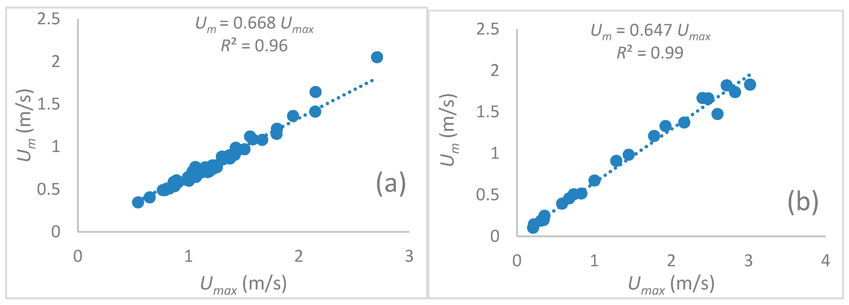
The state equilibrium constants Ω(M) for the Shannon entropy and Ω(G) for the Tsallis entropy, as well as the correlation coefficients were estimated using the pairs of maximum and mean velocities collected at the Pontelagoscuro and Ponte Nuovo stations of the Po and Tiber Rivers, respectively. The estimated values of the state equilibrium constants and correlation coefficients are indicated in Figure 1 using the velocity dataset of the two considered gauge stations.
It can be seen from Figure 1 that the linear relationship established for Pontelagoscuro and Ponte Nuovo stations are Equations (7) and (8), respectively:
The estimate of state equilibrium constant Ω(G) for the Ptelagoscuro station was found to be 0.668 and the corresponding Tsallis entropic constant was G = 4.02. Similarly, the equilibrium estimates of Ω(G) and G for the Ponte Nuovo site of the Tiber River were estimated to be 0.647 and 3.52, respectively.
Ω(G) and G could be assumed to be constant within the river reach [13]. Once the cross-sectional mean flow velocity was estimated by Equations (7) and (8), the discharge could easily be estimated as the product of and the cross-sectional flow area corresponding to the water level observed during the measurement.
The discharge estimation based on the use of Equation (3) could be verified using the values Ω(G) and G separately for both stations. Using Equation (3), one can estimate the maximum flow velocity of a vertical by only measuring the surface flow velocity.
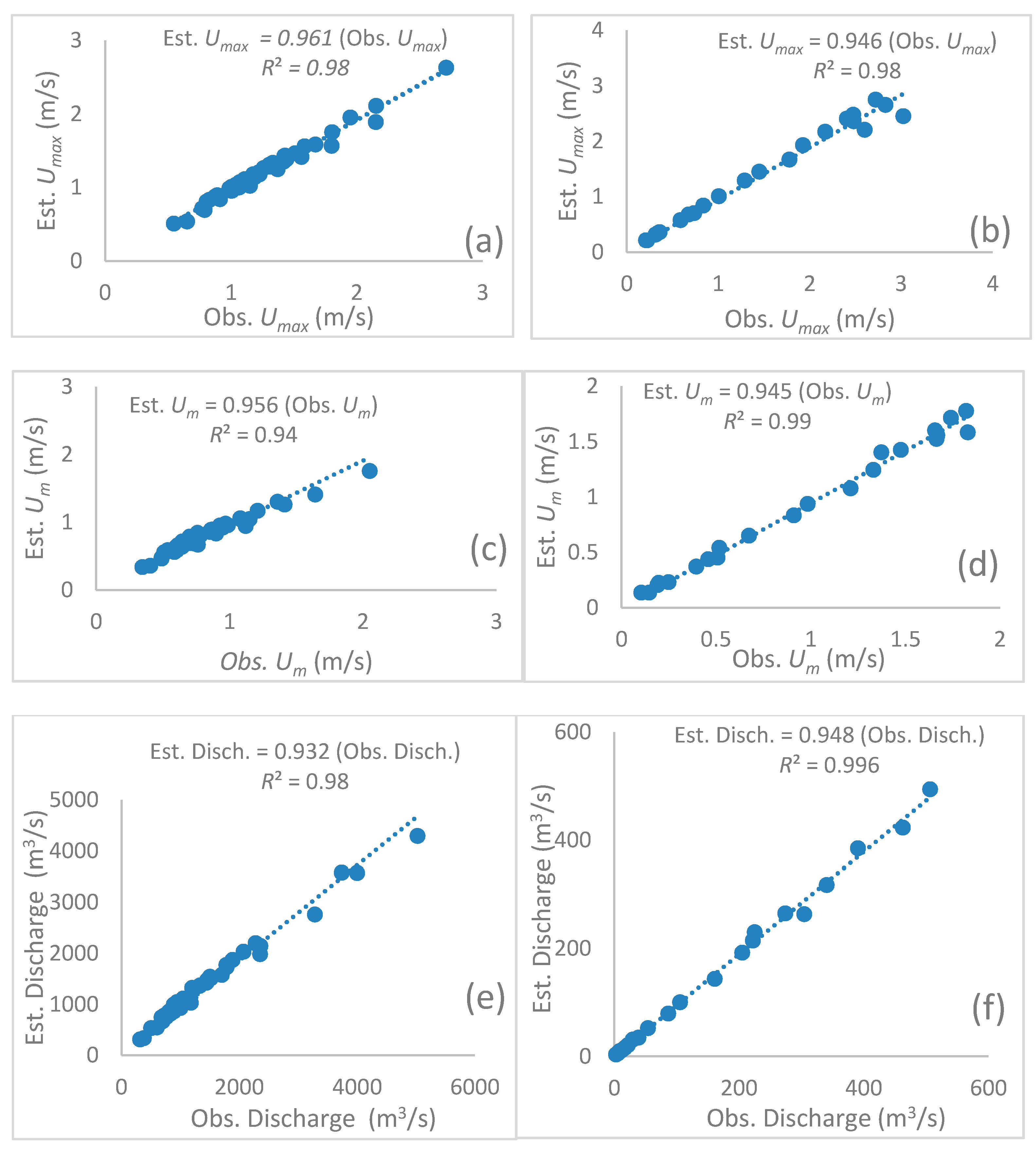
Figure 2a,b compares the estimated maximum velocity based on Tsallis entropy with the corresponding observed maximum velocity for all the events of both the considered gauge stations of the Po and Tiber Rivers using Equation (3). It can be inferred from Figure 2a,b that the values of maximum velocity estimated using Equation (3) closely reproduced the corresponding observed maximum velocity. All velocity estimates were highly correlated (R2 = 0.98 for both the gauge stations) with the observed values. Thefore, the maximum flow velocities estimated by Equation (3) for all the events of both gauge stations were used to assess the cross-sectional mean flow velocity using the Tsallis entropy-based linear relationship in Equation (2).
It can be inferred from Figure 2c,d that the estimated cross-sectional mean flow velocity for all the events of both gauge stations were highly correlated with the corresponding observed values estimated using the velocity–area method [1]. The high values shown in Figure 2c,d imply the acceptability of Equation (3) based on Tsallis entropy theory. Therefore, the cross-sectional mean flow velocity was estimated using Equations (7) and (8), and the discharge was estimated at each of the flow sections by multiplying it with the corresponding cross-sectional flow area.
The discharge values estimated for both gauge stations using the Tsallis entropy-based procedure were highly correlated with the respective station’s observed discharge values, as shown in Figure 2e,f.
4.2. Non-Contact Discharge Assessment Using Shannon Entropy
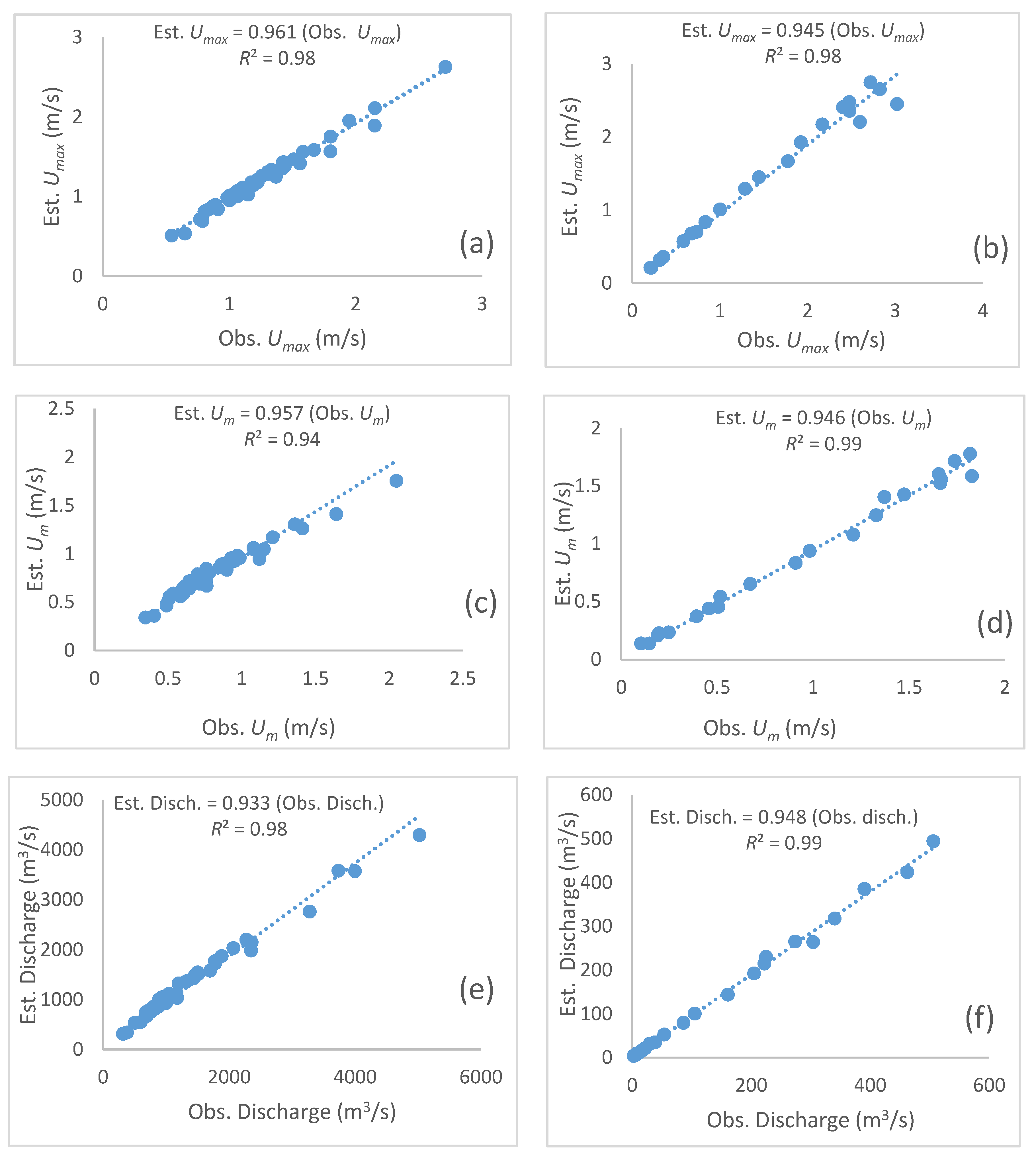
The Tsallis entropy-based mean velocity equation has the same state equilibrium constant as that of Shannon entropy, although the nature of the entropy distribution differs from that of Shannon entropy. We have already estimated the value of the state equilibrium constant Ω(M) as 0.668, as seen from Figure 1, and using Equation (5), we estimated the Shannon entropic constant M = 2.162 for Pontelagscuro gauge station of the Po river and M = 1.87 for the Ponte Nuovo gauge station of the Tiber river.
By using Equation (6), we estimated the maximum flow velocity by starting from the measured surface velocities. Figure 3 demonstrates the closeness of estimated values of maximum velocity, mean velocity, and discharge with the corresponding observed values, as shown in Figure 3a,c,e for the Pontelagoscuro station of the Po River and in Figure 3b,d,f for the Ponte Nuovo station of the Tiber River.
It can be inferred from Figure 2e,f and Figure 3e,f that the discharges estimated based on Tsallis entropy theory compared closely with the discharges estimated using Shannon entropy theory, implying that both methods estimated nearly the same discharge.
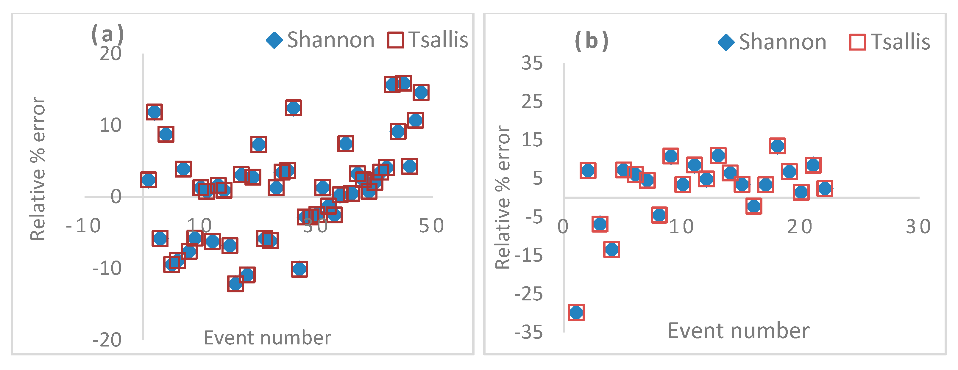
It can be inferred from Figure 4 that by considering the relative error percentage when estimating the cross-sectional mean flow velocity, i.e., × 100, the Tsallis entropy-based procedure compared well with that of the Shannon entropy-based procedure, where
is the computed mean flow velocity and is the observed one.
This finding was also corroborated in Table 2, where the estimates of the Nash–Sutcliffe efficiency (NSE) and the coefficient of determination of both the Tsallis and Shannon entropy-based approaches reproduced the observed discharges very well. Therefore, these results are consistent with those results obtained from previous studies [22,23,24], except with the difference that we employed the measured maximum surface velocity for the discharge estimation using entropy theories. Likewise, the discharge estimates using Tsallis entropy were nearly the same as the discharge estimated using Shannon entropy, and both these estimated discharges closely estimated the discharges obtained using the velocity–area method, with a difference of less than 1% for both the investigated river stations. These inferences demonstrate that both the Shannon and Tsallis entropies can be employed for discharge estimation as alternative methods.
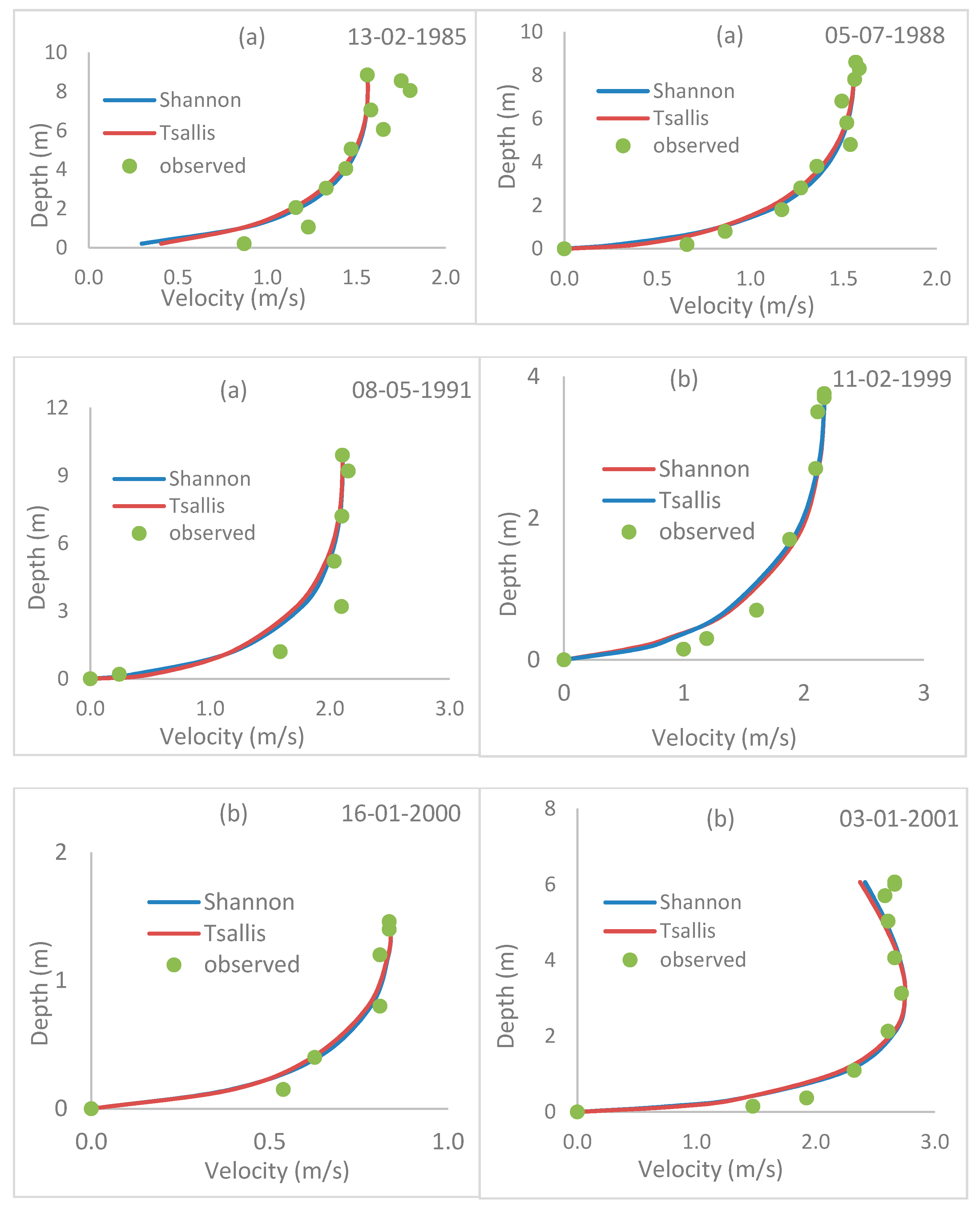
As the study of interest lay with the estimation of the maximum velocity of the vertical velocity profile recorded on the pre-defined points of the y-axis, which in turn is generally located somewhere at the mid-portion of the flow section, where the maximum flow usually passes in a flow section, the y-axis was identified at the observed maximum surface velocity point and subsequently, the dip was observed at this vertical for its use in estimating Umax using Equation (3). The vertical velocity profile at any location of the flow section of a flow event can be estimated using Equation (1) by using the estimated value of instead of the observed value of , such as that depicted by Equation (3) by leveraging the observed surface velocity and the dip. The estimated entropy constants were G = 4.02 for the Pontelagsucro station of the Po River and 3.52 for the Ponte Nuovo station of the Tiber River.
Figure 5 shows the accuracy of the estimated velocity profiles with the observed velocity points for both gauge stations. Similar reproductions were obtained for the other events at both gauge stations. We also generated vertical velocity profiles using Shannon entropy. Our main purpose regarding the vertical velocity profile generation was to compare the generated vertical velocity profiles of both approaches with the corresponding observed vertical profiles. As can be seen from Figure 5 depicting the velocity profiles, there were no significant differences between the performances of the Tsallis and Shannon entropy approaches when estimating the point velocities.
5. Conclusions
Based on the results obtained, the following conclusions can be drawn:
- -
- Non-contact monitoring techniques based on the use of surface flow velocity measurements at river gauge stations by employing surface velocity radar (SVR) and large scale particle image velocimetry (LSPIV) are a valuable alternative approach to the traditional discharge estimation methods. These approaches eliminate the drawbacks of using the traditional methods for monitoring high flow conditions, which prove to be inefficient and subject to accuracy problems, as well as pose safety problems for the operators during high flow conditions. By sampling the maximum surface flow velocity at the y-axis and applying entropy theory, one can accurately estimate the river discharge, which makes the non-contact technology highly appealing for river monitoring. It is worth noting that the uncertainty analysis of entropy-based methods using velocity measurements provide a variation on estimates that, as shown by Alvisi [25], does not exceed 10% on average for high flows. It is also worth noting that recent studies showed that entropy-based models can be applied for any flow conditions using both ground measurements [26,27] and satellite observations [28], and this is of considerable interest for new satellite missions, such as SWOT (Surface Water and Ocean Topography- NASA) and Sentinel (European Space Agency).
- -
- Tsallis entropy theory provided similar performance to the one based on Shannon entropy theory when estimating the cross-sectional mean flow velocity and the velocity profile distribution at the y-axis.
- -
- It was shown that the measure of the surface flow velocity along the y-axis allowed us to efficiently estimate the maximum velocity for which the mean flow velocity can be accurately assessed, regardless of the type of entropy approach applied. The proposed method can be easily replicable for any river site and this finding provides a considerable benefit when using the non-contact techniques for monitoring discharge during any flow conditions, and in particular, during high flow. This is linked to the fact that the key variable Umax can be easily monitored during high flow and the entropy parameter characterizing the slope of the linear entropy relationship does not depend on the hydraulic gradient, which influences the dynamics of flooding. Indeed, as shown by Moramarco and Singh [29], the entropy parameter is linked to the ratio between the geometric and hydraulic characteristics of a river site, which remains constant during a flood.
- -
- Finally, the analysis of velocity profiles at the y-axis showed that by using the observed dip values, both Tsallis and Shannon entropy theories could be used to study the secondary currents when dip phenomena occur. This aspect will be investigated in detail in terms of a two-dimensional velocity distribution when secondary currents occur by using the velocity dataset referring to the gauged river stations with different geometric and hydraulic characteristics and including Indian rivers.
Author Contributions
All authors contributed extensively to the work. J.K.V. performed the numerical experiments, result analyses and participated to write the article. M.P. and T.M. contributed equally to the discussion of methodology, results analysis and the manuscript writing. T.M. promoted and coordinated the research. All authors have read and agreed to the published version of the manuscript.
Funding
This work was partly funded by the MUR-Italian National Research Programme PRIN 2017 within the project “Interactions between hydrodynamics flows and biotic communities in fluvial ecosystems: Advancement in discharge monitoring and understanding of processes relevant for ecosystem sustainability by the development of novel technologies with field observations and laboratory testing (ENTERPRISING).”
Acknowledgments
Authors are grateful to the Department of Environment, Planning, and Infrastructure of Umbria Region and Agenzia Interregionale per il Fiume Po for providing data regarding the Tiber and Po Rivers, respectively. The first author is grateful to the Ministry of Human Resource Development of the Government of India for granting a Research Fellowship for pursuing Doctoral Research at the Department of Hydrology, Indian Institute of Technology Roorkee, Roorkee. The authors are immensely grateful to the reviewers for their useful suggestions, which resulted in the significant improvement of the contents of the paper.
Conflicts of Interest
The authors declare no conflict of interest.
References
- Herschy, R.W. Streamflow Measurement; Elsevier: London, UK, 1985. [Google Scholar]
- Simpson, M.R.; Oltman, R.N. Discharge Measurement System Using a Acoustic Doppler Current Profiler with Applications to Large Rivers and Estuaries. In U.S. Geological Survey Water-Supply Paper; 2395; U.S. Geological Survey: Reston, VA, USA, 1993; 32p. [Google Scholar]
- Fujita, I.; Muste, M.; Kruger, A. Large-scale particle image velocimetry for flow analysis in hydraulic applications. J. Hydraul. Res. 1998, 36, 397–414. [Google Scholar] [CrossRef]
- Tauro, F.; Porfiri, M.; Grimaldi, S. Orienting the camera and firing lasers to enhance large scale particle image velocimetry for streamflow monitoring. Water Resour. Res. 2014, 50, 7470–7483. [Google Scholar] [CrossRef]
- Costa, J.E.; Spicer, K.R.; Cheng, R.T.; Haeni, F.P.; Melcher, N.B.; Thurman, E.M. Measuring stream discharge by non-contact methods: A proof-of-concept experiment. Geophys. Res. Lett. 2000, 27, 553–556. [Google Scholar] [CrossRef]
- Welber, M.; Le Coz, J.; Laronne, J.B.; Zolezzi, G.; Zamler, D.; Dramais, G.; Hauet, A.; Salvaro, M. Field assessment of noncontact stream gauging using portable surface velocity radars (SVR). Water Resour. Res. 2016, 52, 1108–1126. [Google Scholar] [CrossRef] [Green Version]
- Muste, M.; Fujita, I.; Hauet, A. Large-scale particle image velocimetry for measurements in riverine environments. Water Resour. Res. 2008, 44, W00D19. [Google Scholar] [CrossRef] [Green Version]
- Chiu, C.-L. Velocity distribution in open channel flow. J. Hydraul. Eng. 1989, 115, 576–594. [Google Scholar] [CrossRef]
- Chiu, C.-L.; Hsu, S.H.; Tung, N.-C. Efficient methods of discharge measurements in rivers and streams based on the probability concept. Hydrol. Process. 2005, 19, 3935–3946. [Google Scholar] [CrossRef]
- Chiu, C.-L.; Tung, N.-C. Maximum velocity and regularities in open-channel flow. J. Hydraul. Eng. 2002, 128, 390–398. [Google Scholar] [CrossRef]
- Shannon, C.E. A mathematical theory of communication. Bell Syst. Tech. J. 1948, 27, 623–656. [Google Scholar] [CrossRef]
- Jaynes, E.T. Information theory and statistical mechanics I. Phys. Rev. 1957, 106, 620–630. [Google Scholar] [CrossRef]
- Xia, R. Relation between mean and maximum velocities in a natural river. J. Hydraul. Eng. ASCE 1997, 123, 123,720–723. [Google Scholar] [CrossRef]
- Moramarco, T.; Saltalippi, C.; Singh, V.P. Estimation of mean velocity in natural channel based on Chiu’s velocity distribution equation. J. Hydrol. Eng. 2004, 9, 42–50. [Google Scholar] [CrossRef]
- Mirauda, D.; Pannone, M.; De Vincenzo, A. An entropic model for the assessment of streamwise velocity dip in wide open channels. Entropy 2018, 20, 69. [Google Scholar] [CrossRef] [Green Version]
- Stearns, F.P. On the current meter, together with a reason why the maximum velocity of water flowing in open channel is below the surface. Trans. Am. Soc. Civ. Eng. 1883, 3, 20–32. [Google Scholar]
- Termini, D.; Moramarco, T. Dip phenomenon in high-curved turbulent flows and application of entropy theory. Water 2018, 10, 306. [Google Scholar] [CrossRef] [Green Version]
- Fulton, J.; Ostrowski, J. Measuring real-time streamflow using emerging technologies: Radar, hydroacoustics, and the probability concepts. J. Hydrol. 2008, 357, 1–10. [Google Scholar] [CrossRef]
- Moramarco, T.; Barbetta, S.; Tarpanelli, A. From Surface Flow Velocity Measurements to Discharge Assessment by the Entropy Theory. Water 2017, 9, 120. [Google Scholar] [CrossRef] [Green Version]
- Tsallis, C. Possible generalization of Boltzmann-Gibbs statistics. J. Stat. Phys. 1988, 52, 479–487. [Google Scholar] [CrossRef]
- Singh, V.P. Introduction to Tsallis Entropy Theory in Water Engineering; CRC Press/Taylor and Francis: Boca Raton, FL, USA, 2016. [Google Scholar]
- Cui, H.; Singh, V.P. One-dimensional velocity distribution in open channels using Tsallis entropy. J. Hydrol. Eng. 2014, 19, 290–298. [Google Scholar] [CrossRef]
- Cui, H.; Singh, V.P. Two-dimensional velocity distribution in open channels using the Tsallis entropy. J. Hydrol. Eng. 2013, 18, 331–339. [Google Scholar] [CrossRef]
- Singh, V.P.; Luo, H. Entropy theory for distribution of one-dimensional velocity in open channels. J. Hydrol. Eng. 2011, 16, 725–735. [Google Scholar] [CrossRef]
- Alvisi, S.; Barbetta, S.; Franchini, M.; Melone, F.; Moramarco, T. Comparing grey formulations of the velocity-area method and entropy method for discharge estimation with uncertainty. J. Hydroinf. 2014, 16, 797–811. [Google Scholar] [CrossRef]
- Alimenti, F.; Bonafoni, S.; Gallo, E.; Palazzi, V.; Vincenti Gatti, R.; Mezzanotte, P.; Roselli, L.; Zito, D.; Barbetta, S.; Corradini, C.; et al. Non-Contact Measurement of River Surface Velocity and Discharge Estimation with a Low-Cost Doppler Radar Sensor. IEEE Trans. Geosci. Remote Sens. 2020, 1–13. [Google Scholar] [CrossRef]
- Fulton, J.W.; Mason, C.; Eggleston, J.; Nicotra, M.; Chiu, C.L.; Henneberg, M.; Best, H.; Cederberg, J.; Holnbeck, S.; Lotspeich, R.; et al. Remote Sensing of Surface Velocity and River Discharge Using Radars and the Probability Concept at 10 USGS Streamgages. Remote Sens. 2020, 12, 1296. [Google Scholar] [CrossRef] [Green Version]
- Moramarco, T.; Barbetta, S.; Bjerklie, D.M.; Fulton, J.W.; Tarpanelli, A. River Bathymetry Estimate and Discharge Assessment from Remote Sensing. Water Resour. Res. 2019, 55, 6692–6711. [Google Scholar] [CrossRef]
- Moramarco, T.; Singh, V.P. Formulation of the entropy parameter based on hydraulic and geometric characteristics of river cross sections. J. Hydrol. Eng. 2010, 15, 852–858. [Google Scholar] [CrossRef]
Figure 1.
The relation between the cross-sectional mean flow velocity Um and the maximum velocity Umax for (a) Pontelagoscuro station and (b) Ponte Nuovo station.
Figure 1.
The relation between the cross-sectional mean flow velocity Um and the maximum velocity Umax for (a) Pontelagoscuro station and (b) Ponte Nuovo station.

Figure 2.
Comparison of pertinent estimated variables with the corresponding observed ones using Tsallis entropy for Ponteslagscuro station (a,c,e) and Ponte Nuovo (b,d,f).
Figure 2.
Comparison of pertinent estimated variables with the corresponding observed ones using Tsallis entropy for Ponteslagscuro station (a,c,e) and Ponte Nuovo (b,d,f).

Figure 3.
Comparison of the pertinent estimated variables with the corresponding observed ones using Shannon entropy for Ponteslagscuro station (a,c,e) and Ponte Nuovo (b,d,f).
Figure 3.
Comparison of the pertinent estimated variables with the corresponding observed ones using Shannon entropy for Ponteslagscuro station (a,c,e) and Ponte Nuovo (b,d,f).

Figure 4.
The relative percentage error in estimating the cross-sectional mean velocity using Tsallis and Shannon entropies: (a) Pontelagscuro and (b) Ponte Nuovo.
Figure 4.
The relative percentage error in estimating the cross-sectional mean velocity using Tsallis and Shannon entropies: (a) Pontelagscuro and (b) Ponte Nuovo.

Figure 5.
Typical velocity profiles estimated using Tsallis and Shannon entropies, and a comparison with the observed velocity points (depth (y-axis) represents the vertical where occurs) for the gauging stations at (a) Pontelagscuro and (b) Ponte Nuovo.
Figure 5.
Typical velocity profiles estimated using Tsallis and Shannon entropies, and a comparison with the observed velocity points (depth (y-axis) represents the vertical where occurs) for the gauging stations at (a) Pontelagscuro and (b) Ponte Nuovo.


Table 1.
Flow data set details: —number of events considered, —total number of verticals (from the events), Q—measured discharge, D—dep, A—area.
Table 1.
Flow data set details: —number of events considered, —total number of verticals (from the events), Q—measured discharge, D—dep, A—area.
| River | Station | Q (m3/s) | D (m) | A (m2) | Period | ||
|---|---|---|---|---|---|---|---|
| Po | Pontelagoscuro | 48 | 595 | 316–5026 | 5.41–15.46 | 913–2833 | 1984–1992 |
| Tiber | Ponte Nuovo | 22 | 186 | 2.65–506 | 0.91–6.07 | 25.48–278.16 | 1985–2000 |
Table 2.
Estimated percentage of errors in estimating the mean flow velocity using Tsallis and Shannon entropy and using only the observed surface velocities.
Table 2.
Estimated percentage of errors in estimating the mean flow velocity using Tsallis and Shannon entropy and using only the observed surface velocities.
| Metrics | Pontelagscuro | Ponte Nuovo | ||
|---|---|---|---|---|
| Tsallis | Shannon | Tsallis | Shannon | |
| Mean (%) | 5.59 | 5.59 | 7.55 | 7.58 |
| Standard Deviation (%) | 6.95 | 6.95 | 8.79 | 8.49 |
| NSE * | 0.99 | 0.99 | 0.99 | 0.99 |
| 0.98 | 0.98 | 0.99 | 0.99 | |
* NSE: Nash–Sutcliffe efficiency.
© 2020 by the authors. Licensee MDPI, Basel, Switzerland. This article is an open access article distributed under the terms and conditions of the Creative Commons Attribution (CC BY) license (http://creativecommons.org/licenses/by/4.0/).
Share and Cite
MDPI and ACS Style
Vyas, J.K.; Perumal, M.; Moramarco, T. Discharge Estimation Using Tsallis and Shannon Entropy Theory in Natural Channels. Water 2020, 12, 1786. https://doi.org/10.3390/w12061786
AMA Style
Vyas JK, Perumal M, Moramarco T. Discharge Estimation Using Tsallis and Shannon Entropy Theory in Natural Channels. Water. 2020; 12(6):1786. https://doi.org/10.3390/w12061786
Chicago/Turabian StyleVyas, Jitendra Kumar, Muthiah Perumal, and Tommaso Moramarco. 2020. "Discharge Estimation Using Tsallis and Shannon Entropy Theory in Natural Channels" Water 12, no. 6: 1786. https://doi.org/10.3390/w12061786
Note that from the first issue of 2016, this journal uses article numbers instead of page numbers. See further details here.