Pier Scour Prediction in Non-Uniform Gravel Beds


1
Department of Civil Engineering, National Institute of Technology Warangal, Warangal 506004, India
2
School of Engineering, University of Basilicata, 85100 Potenza, Italy
3
School of Civil Engineering, University of Bradford, Bradford BD7 1DP, UK
4
Department of Civil Engineering, Indian Institute of Technology Roorkee, Roorkee 247667, India
*
Author to whom correspondence should be addressed.
Water 2020, 12(6), 1696; https://doi.org/10.3390/w12061696
Submission received: 24 May 2020
/
Revised: 8 June 2020
/
Accepted: 10 June 2020
/
Published: 13 June 2020
(This article belongs to the Special Issue Bridge Hydraulics: Current State of the Knowledge and Perspectives)
Abstract
:Pier scour has been extensively studied in laboratory experiments. However, scour depth relationships based on data at the laboratory scale often yield unacceptable results when extended to field conditions. In this study, non-uniform gravel bed laboratory and field datasets with gravel of median size ranging from 2.7 to 14.25 mm were considered to predict the maximum equilibrium scour depth at cylindrical piers. Specifically, a total of 217 datasets were collected: 132 from literature sources and 85 in this study using new experiments at the laboratory scale, which constitute a novel contribution provided by this paper. From the analysis of data, it was observed that Melville and Coleman’s equation performs well in the case of laboratory datasets, while it tends to overestimate field measurements. Guo’s and Kim et al.’s relationships showed good agreements only for laboratory datasets with finer non-uniform sediments: deviations in predicting the maximum scour depth with non-uniform gravel beds were found to be significantly greater than those for non-uniform sand and fine gravel beds. Consequently, new K-factors for the Melville and Coleman’s equation were proposed in this study for non-uniform gravel-bed streams using a curve-fitting method. The results revealed good agreements between observations and predictions, where this might be an attractive advancement in overcoming scale effects. Moreover, a sensitivity analysis was performed to identify the most sensitive K-factors.
1. Introduction
One of the key factors for bridge stability is the scour around piers and abutments, which is caused by flowing water. Scour is a natural but complicated phenomenon in river engineering due to the three-dimensional flow separations around bridge elements, the natural bed forms, the existence of vegetation, and the complex natural flow conditions [1,2,3,4,5]. Recent surveys have shown that in a sample of about 500 bridges collapsed in the US since 1951, 60% of collapses were due to pier scour [6,7]. Qi et al. [5] performed a field scour analysis and came to the conclusion that the access allowance through the embankment and scour at bridge foundations are the main causes of bridge failure. Therefore, the estimation of the amount of scour is necessary for designing an economical and safe bridge structure [1,8,9,10].
The scour hole around the pier usually develops due to the primary vortex, which is caused by hydrodynamic drag and lift forces on sediment particles near the pier; the particles are then carried downstream of the pier [11,12]. The transportation of particles near the bridge elements usually occurs layer by layer [13] and the scour depth around a bridge pier depends on various flow and sediment properties [9,11,13,14,15,16,17]. Previous studies recognized the discrepancy between experimental and field scour depth measurements, which is mainly due to the scaling effects from laboratory tests [3,5]. Moreover, these differences could also be due to the difficulties during field data collection, instability of flow conditions, and variations in streambed particles [3,8].
In terms of flow conditions, the local scour for both clear-water and live-bed conditions has been extensively studied and several approaches, along with mathematical relationships, have been found [2,3,4,8,12]. Numerous studies have been completed to calculate the scour depth around the bridge piers [3,5,7,9,10,11,12,13,14,15,16,17]. Most of these studies were conducted for uniform sediment beds and several relationships were developed after analyzing the experimental datasets at the laboratory scale only. However, very few studies are available for non-uniform coarser beds [9,11,14].
Several studies for pier and abutment scours were completed by researchers over non-uniform sediment beds [15,16,17,18,19,20,21,22]. However, very few studies are available for non-uniform gravel beds. Raikar and Dey [15] stated that the maximum scour depth at the equilibrium stage increases with a decrease in particle size for both uniform and non-uniform gravels. For non-uniform sediments, the influence of coarser particles on the equilibrium scour depth is also prominent [15]. The equilibrium scour depth in non-uniform sediment beds is noteworthy and prevents the development of a scour hole by forming an armor layer [15]. Jueyi et al. [17] conducted 50 flume experiments for semi-circular and semi-elliptical abutments under different flow conditions and sediment sizes. They proposed an empirical equation to compute the maximum scour depth at an equilibrium condition. The scour hole at an equilibrium condition is not dependent on either the condition of the armor layer or the bed material [17]. Abderrezzak et al. [18] checked the scale effects of non-uniform sediment on sediment transport that preserves the similarity of incipient motion of the particle size and the bank stability. The time factor for sediment transport and mass movement depends on the flow rate and sediment size [18]. Pournazeri et al. [19] developed a three-dimensional pier scour prediction model for scour using non-uniform laboratory experimental data. They allowed for selective non-uniform sediment transport around the pier to calculate the scour rate and stated that the scour pattern emerges from the adjacent sides of the pier and slowly migrates toward the upstream nose of the pier. The non-uniformity of sediments reduces the size of the scour hole [19]. Sharma et al. [20] investigated the multi-scale statistical characterization of a migrating pier scour pattern over non-uniform sediment beds. Experimentally, it was observed that the turbulent characteristics at the upstream of the scour hole were negative, while the occurrence of downward seepage stabilizes the reversal of the flow and results in reduced turbulence characteristics. Pandey et al. [21] conducted flume experiments under clear-water scour conditions and analyzed the equilibrium pier scour processes in non-uniform gravel beds. They proposed a graphical method for calculating the maximum scour depth under an equilibrium condition. The scour hole occurs via the creation of an armor layer in non-uniform sediment beds and the equilibrium scour condition is achieved when a steady armor layer forms around the pier [21].
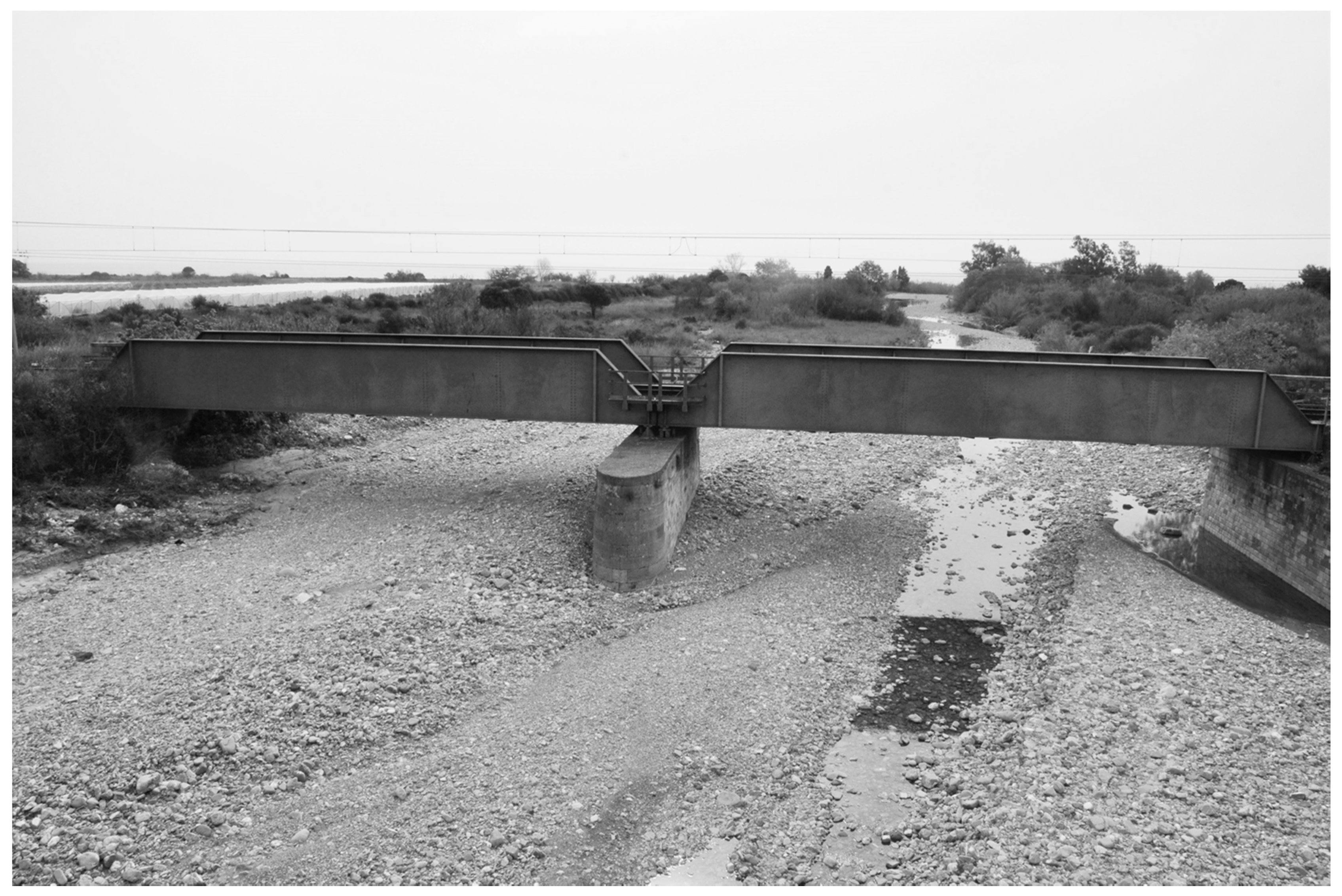
The pier scour and processes under uniform gravel beds have been studied extensively and are well documented. However, these studies did not emphasize the significance of the scour evolution in non-uniform gravel-bed streams. Therefore, in this study, we aimed to predict the maximum scour depth in equilibrium condition over non-uniform sediment beds. Herein, a difference was recognized between non-uniform gravels and non-uniform finer sediments. Figure 1 provides an example of a bridge on a gravel-and-cobble-bed stream. Signs of local erosion were noticeable at the right abutment and could just be noticed at the front of the central pier.
In particular, this study focused on local scour around circular piers under clear-water conditions. It aims to provide an approach for the estimation of the maximum scour depth at the equilibrium conditions at piers founded into non-uniform gravels; this was done based on both laboratory and field datasets. The paper is then organized to achieve the following main objectives: (i) to assess the performance of selected approaches from the literature, (ii) to propose a simplified but effective clear-water scour approach in terms of crucial factors considering flow–pier–sediment interactions, and then (iii) to verify such an approach using a wide-ranging dataset from the literature and novel experiments carried out in the present study.
2. Materials and Methods
2.1. Experiments
In the present study, 85 new laboratory experiments were carried out to investigate non-uniform gravel beds. Furthermore, 132 datasets (77 flume experimental and 55 field datasets) from literature sources [15,23,24,25,26] were collected and analyzed to extend the range of applicability of a new approach that will hereafter be introduced. All these datasets, 217 in total, were also used to analyze and discuss the accuracy of selected approaches from the published literature.
2.1.1. Experimental Works from Literature Sources
The experimental/field data collected by Raikar and Dey [15], Kothyari [23], Kumar [24], Lodhi [25], and Benedict and Caldwell [26] were considered in this study. Table 1 shows the ranges for the main dimensional parameters.
Kothyari [23] carried out a flume experimental study to estimate scour depth variations under live-bed scour and clear-water scour conditions. All tests were completed in a 30 m long and 1 m wide fixed bed masonry flume. Non-uniform sediment with a median grain size d50 = 8.30 mm and sediment gradation σ = 1.80 was used. He used circular galvanized hollow iron pipes of diameter b = 0.05–0.11 m as the pier model. The value of the threshold velocity ratio (U/Uc) and approach flow depth (y) under clear-water scour conditions were kept between 0.70–0.95 and 0.06–0.13 m, respectively.
Kumar [24] carried out an experimental series in a 20 m long and 1 m wide fixed masonry flume. He completed all the tests under the clear-water conditions for two different non-uniform gravels of d50 = 3.47–4.0 mm and σ = 1.52–1.67. Four different circular piers of cast iron with b = 0.05–0.20 m were used. He used a point gauge for measuring the maximum equilibrium scour depth over the final bed topography. All tests were conducted for a fixed duration of 8 h.
Lodhi [25] carried out flume tests in a 26 m long and 2.0 m wide rectangular flume. He used five different circular pier model with b = 0.08–0.25 m. Five different non-uniform sediments of d50 = 2.7–5.53 mm and σ = 1.43–1.51 were considered. The maximum equilibrium scour depth was measured at the upstream nose of the pier with a point gauge. It was observed that the equilibrium scour depth was reached within 12 h.
Raikar and Dey [15] conducted an experimental study on square and circular piers in uniform and non-uniform sediments (fine and medium gravels) under clear-water conditions. All tests were completed in a rectangular flume that was 12 m long and 0.6 m wide. Fifteen different non-uniform sediments with d50 = 4.10–14.25 mm and σ = 1.43–2.90 were used. It was observed that the maximum scour depth at the equilibrium condition increases with a decrease in the median diameter of sediments. They concluded that the resulting gravel size factors, found using envelope curve fitting, were notably different from the previous studies. The effect of sediment non-uniformity function on the maximum scour depth was also noticeable in non-uniform gravels.
The United State Geological Survey (USGS) completed a state-of-the-art study on pier scour to recognize possible sources of available pier scour data. These USGS datasets consisted of around 1800 field observations for bridge piers and abutments under clear-water and live-bed scour conditions. In this study, we used only the non-uniform sediment data under clear-water conditions. These datasets cover an extensive range of field conditions and illustrate field datasets from 23 states within the U.S. and 6 from other countries.
In terms of dimensionless parameters and the approach flow conditions, the Reynolds number ranged from 1.65 × 10⁵ to 2.53 × 10⁵, 1.04 × 10⁵ to 1.24 × 10⁶, 3.8 × 10⁵ to 5.1 × 10⁶, 3.3 × 10⁵ to 5.2 × 10⁵ and 1.48 × 10⁴ to 3.4 × 10⁷; the Froude number ranged from 0.22 to 0.42, 0.47 to 0.71, 0.22 to 0.34, 0.21 to 0.75, and 0.06-0.50; and the densimetric Froude number ranged from 2.13 to 2.67, 2.31 to 2.95, 1.47 to 3.48, 1.33 to 3.56, and 1.86 to 12.37 for Kothyari [23], Raikar and Dey [15], Kumar [24], Lodhi [25], and Benedict and Caldwell [26], respectively.
2.1.2. Present Experimental Work
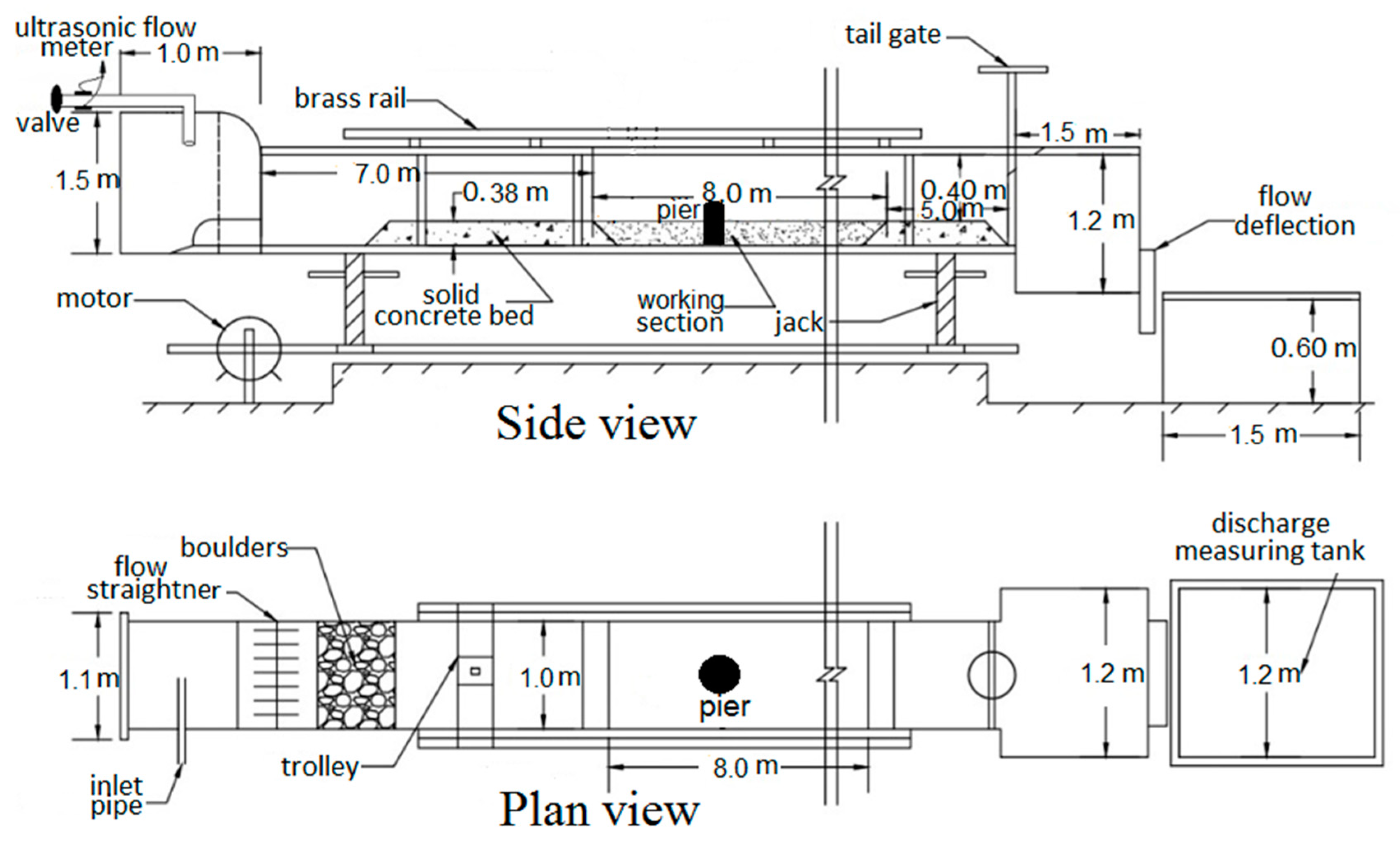
Experiments were carried out in a rectangular flume that was 20 m long, 1 m wide, and 0.78 m deep. The working-section with a length of 8 m, a width of 1 m, and a depth of 0.38 m started at a distance of 7 m from the flume entrance to allow for fully developed flows. Figure 2 shows a side and a plan view of the experimental setup.
The working section was filled with one of eight non-cohesive, non-uniform sediments with a median grain size (d50) equal to 3.26 mm, 3.82 mm, 4.38 mm, 4.94 mm, 7.50 mm, 8.60 mm, 9.10 mm, or 10.70 mm; geometric standard deviation (σ = d84/d16)1/2 equal to 1.59, 1.71, 1.88, 1.51, 1.56, 1.63, 1.66, and 1.57, respectively; and with a 2.65 relative density (S). d84 and d16 are the particle sizes at 84% and 16% finer, respectively. These sediments were filled-up to the level of the flume bed and a 2-D profiler was used to level the mobile bed. Four different hollow cylinders were used as uniform circular pier models with a diameter (b) equal to 6.6 cm, 8.4 cm, 11.5 cm, and 13.5 cm. A valve fixed at the inlet pipe controlled the flow discharge. An ultrasonic flow meter measured the flow discharge in the flume. The maximum scour depth at the quasi-equilibrium conditions (dse) was measured with a point gauge. All the experiments were conducted for 24 h or more to obtain quasi-equilibrium conditions. However, the equilibrium time varied in the range of 10–16 h. To confirm that an equilibrium scour condition was present, we measured the scour depth every 30 min, and as long as no differences of scour depths with time were observed with an accuracy of ±1 mm, an equilibrium was assumed. However, the equilibrium scour condition around piers in gravel beds depends on the particle size and flow conditions such that the time to reach such conditions is expected to decrease significantly with increasing particle size. This is also due to the reduction of the erosive power of the horseshoe vortex because of the dissipation of its energy through the interstices of the particles [12]. Therefore, the duration of the run was also compared to the conditions of end scour based on the approach used by Kothyari et al. [16], as will be shown below in Table 1, to better corroborate the empirical evidence. Here, te represents the equilibrium time for the present experimental observations and t* represents the equilibrium scour time found by Kothyari et al. [16].
Before starting each experiment, the pier model was fixed vertically across the flow at the center of the working section. This working section was perfectly finished and leveled relative to the longitudinal slope of the flume bed and then covered with a Perspex sheet. Once the predetermined flow condition was established, the Perspex sheet was removed carefully to avoid scour during this process. The hydraulic parameters and scour depth data for each experiment are given in Table 2. It was observed that dse around the pier always occurred at the upstream pier nose and the scour hole geometry was similar at the left and right sides of the pier. Similar findings have also been found by many researchers [2,27,28,29].
In Table 2, y is the approach flow depth, U is the time-averaged approach flow velocity, and Uc is the critical velocity when sediment begins to move. It can be easily recognized that the pier diameter b ranged from 0.07 to 0.14 m, the grain size d50 ranged from 3.26 to 10.70 mm, the sediment gradation σ ranged from 1.51 to 1.88, the flow depth y ranged from 0.10 to 0.14 m, the flow velocity U ranged from 0.44 to 0.79 m/s, and the ratio U/Uc ranged from 0.71 to 0.98 (i.e., clear-water scour regime). In terms of the dimensionless parameters and the approach flow conditions, it can also be recognized that the Reynolds number (Re) ranged from 6.7 × 10⁵ to 7.9 × 10⁵, the Froude number (Fr) ranged from 0.43 to 0.72, and the densimetric Froude number (Fd) ranged from 1.63 to 2.35.
Therefore, the approach flow Reynolds number was always greater than 105, thereby ensuring fully turbulent flow conditions; the sediment grain sizes were such that viscosity effects at the flow-sediment interface could be neglected [28,30]; the ratio of the flume width to the approach flow depth was kept greater than 5 to minimize side-wall effects [31]; and the ratio of the flume width to the pier diameter was always greater than or close to 10 to inhibit contraction/blockage effects [32].
Table 2 also shows that the experiments were systematically conducted: eight non-cohesive, non-uniform sediments were considered; four cylindrical piers were used for each sediment; and finally, for a given sediment and a given cylindrical pier, three flow intensities were created by changing the approach flow depth and/or the discharge.
2.2. Predictive Approaches from Literature
In this study, the maximum scour depths were first analyzed using literature approaches. Three commonly cited maximum pier scour depth relationships for non-uniform sediment beds were considered, namely those of Guo [9], Melville and Coleman [11], and Kim et al. [14].
2.2.1. Melville and Coleman’s Approach
Melville and Coleman [11] proposed an approach to estimate the local scour depth at bridge piers primarily based on controlling factors, termed K-factors, which account for the effects of flow depth; flow intensity; sediment characteristics; approach channel geometry; and foundation type, size, shape, and alignment. The K-factors were estimated by fitting the enveloping curves to the experimental data. Specifically, the scour depth at the equilibrium stage, dse, is the result of the combination of various K-factors, as follows:
where Kby is the flow depth–pier diameter/width factor, KI is the flow intensity factor, Kd50 is the sediment size factor, KS is the pier shape factor, Kθ is the pier alignment factor, and Kσ is the sediment uniformity/non-uniformity factor. For circular piers, as exemplified in this study, both the values of the shape factor KS and the alignment factor Kθ are equal to 1.
For computing Kby, Melville and Coleman [11] proposed a specific relationship depending on the range of b/y values, as follows:
The value of KI depends on the approach flow velocity and critical flow velocity of the streambed particles. Hence, KI accounts for the effect of the flow intensity on the maximum scour. It also accounts for the non-uniformity of bed sediment in terms of the armor peak velocity (Ua). It is given as:
where Uc and Ua are computed according to Melville and Sutherland [33] using the following relationship:
where u*c is the critical shear velocity, calculated using Shield’s approach, and Ua = 0.8Uca. Uca is the critical armor velocity and can be calculated using Equation (4). For computing Uca, Uc is replaced by Uca and u*c is replaced by u*ca. u*ca is calculated by considering the Shield’s approach.
Based on the pier data from Ettema [12], Chiew [34], and Baker [35], the envelope curves defining the sediment size factor Kd50 have the following equations:
Equations (5) were found to be identical for both uniform and non-uniform sediments on the condition that d50 for non-uniform sediments is the median size of the armor layer.
Finally, the factor Kσ is defined as:
2.2.2. Guo’s Approach
Guo [9] has proposed the following conservative equation for the prediction of clear-water scour at the equilibrium stage in the case of singular circular piers in non-cohesive sediment mixtures:
where H is the so-called Hager’s number representing the effect of the reduced gravity ((ρs/ρ) − 1)g on the water-sediment interface, where ρ is the water density, ρs the sediment density, and g the gravitational acceleration; this is similar to the classic Froude number representing the effect of the gravity g on water-air interfaces [9]. Equation (7) was tested using flume data with d50 ranging from 0.55 to 16.7 mm and σ from 1.3 to 3.4. However, the author emphasized that his study was based on a limited database and more experimental data, as well as further analyses, would be needed for a more exhaustive understanding of pier scour for sediment mixtures under a clear-water regime [9].
2.2.3. Kim et al.’s Approach
Kim et al. [14] proposed a design method for bridge piers, and the results of this study were compared to various existing methods for pier design. They used equilibrium scour data from the literature for validation. Support vector machine (SVM) and non-dominated sorting genetic algorithm (NSGA-II) approaches were also used for deriving maximum scour depth relationships. The proposed relationship was compared with two selected empirical models. The outcomes showed that their proposed relationship improved the estimation of the maximum scour depth under an equilibrium scour condition, where their proposed relationship is shown below:
where Fr is the Froude number. Generally, the performance of the NSGA-II based relationship depends on the crossover probability, crossover index, population size, mutation index, and mutation probability [14]. Equation (8) was derived using limited field data (from only 30 trials) with d50 = 0.12–11.0 mm and σ = 1.2–20.34. The accuracy of their model can be increased by increasing the number of trial datasets.
3. Results and Discussion
In this section, both the laboratory and field datasets from the literature sources shown in Table 1 are considered. First, the performances of some literature approaches are assessed and then a new approach is proposed, the performance of which looks promising.
3.1. Comparative Analysis for Previous Approaches
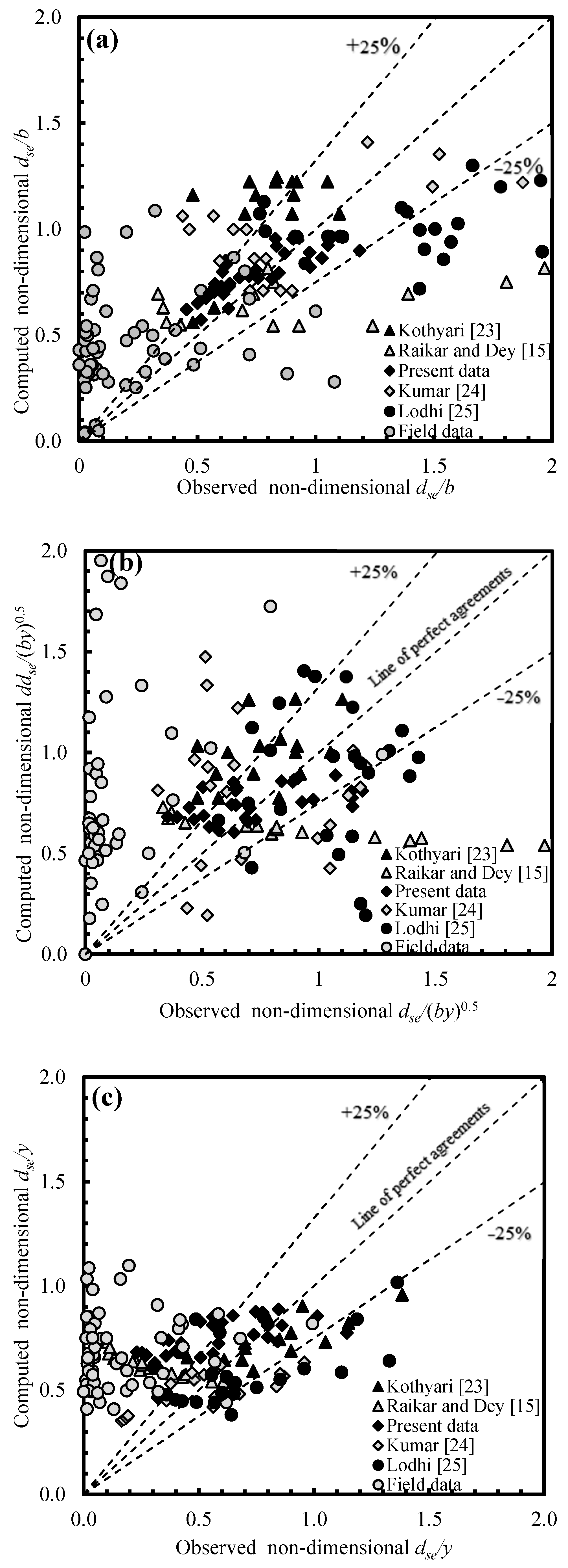
Figure 3a–c demonstrates the percentage errors between the calculated and observed experimental/field scour depths for Melville and Coleman’s [11], Guo’s [9], and Kim et al.’s [14] approaches, respectively, with ±25% error bands. Figure 3a, relating to the Melville and Coleman’s [11] approach, shows the findings for the calculated values of the normalized maximum scour depth, dse/b, with about 40% of the datasets falling inside the ±25% error margins. A reasonable accuracy was found especially for fine-sized gravel data. Figure 3c refers to the approach by Kim et al. [14]. The comparison between the observed and computed values of dse/y revealed that 22% of datasets were within the ±25% errors. In the case of Guo’s [9] approach (Figure 3b), only 20% of datasets of dse/(by)0.5 were within the ±25% errors. It should be noted that different normalizing parameters were used for dse according to the scale-length parameter used in the specific approach. This, of course, would not affect the results of the comparison.
Guo’s [9] equation only showed good agreement for relatively fine sediments (Figure 3b). When this equation was analyzed for coarser experimental and field data, it showed more significant errors: around 95% of field data were found outside the ±25% error bands. The analyses that were used here revealed that Guo’s [9] equation only appeared applicable to laboratory datasets. Kim et al. [14] used the approach flow depth to normalize the maximum scour depth, which affected the accuracy of their equation. Instead, Melville and Coleman [11] considered both non-uniform coarse sand and fine gravel to derive their equation. Therefore, this approach seemed to perform better with the data considered in this study.
3.2. A New Approach for the Maximum Equilibrium Scour Depth
In an attempt to propose a new approach for the prediction of the maximum scour depth, 70% of the entire set of data was used for calibration and the remaining 30% was used for validation. Moreover, the laboratory and field datasets were analyzed and validated separately.
Equation (1) proposed by Melville and Coleman [11] was obtained by considering both the non-uniform sand and non-uniform fine gravel. Here, the K-factors proposed by them were revised using an enveloping curve-fitting method and incorporating new non-uniform gravel laboratory datasets (mainly collected in this study) and field datasets. Above all, the analysis of data revealed that Equation (1) should be modified to:
where the 0.5 factor can be explained as a correction factor for a circular pier. The revised K-factors are given through Equations (10)–(12) below. The values of the shape factor Ks and alignment factor Kθ were both set equal to 1 because circular piers were considered.
3.2.1. Flow Depth–Pier Diameter Factor (Kby)
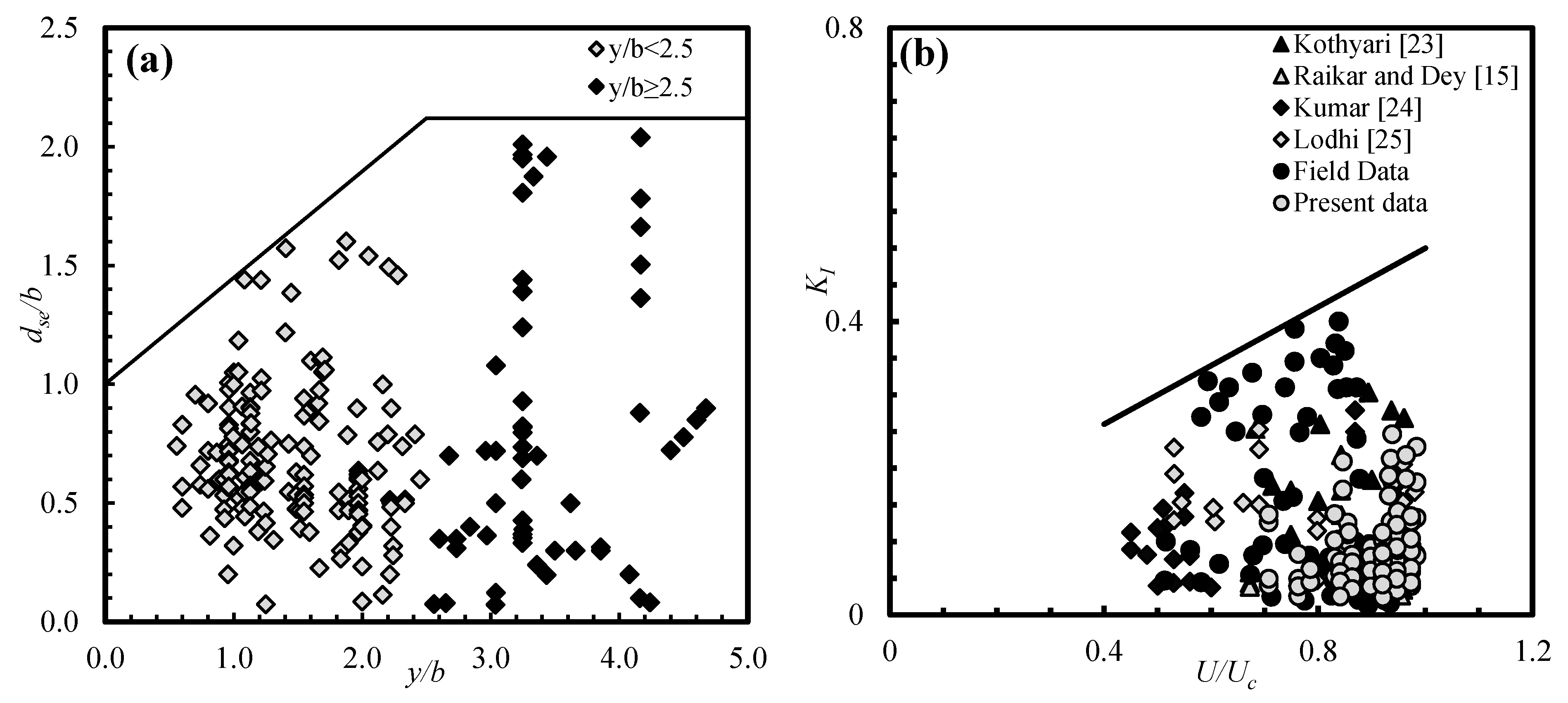
From the variation of d*se = dse/b against y* = y/b, an asymptotic variation of the scour depth with different approach flow depths was identified. Data for single circular piers from laboratory and field studies were arranged and shown in Figure 4a for various flow conditions. The factor Kby is the value of d*se at a specific point of y*. As illustrated in Figure 4a, the enveloping curve for 70% non-uniform calibrating gravel bed data gave a ratio factor Kby of:
3.2.2. Flow Intensity Factor (KI)
The flow intensity factor is known as the ratio of the maximum equilibrium scour depth at a particular flow velocity to its value at the critical velocity. For uniform (σ ≤ 1.4) and non-uniform sediments (σ > 1.4), the U/Uc ratio is a factor of the flow intensity measurement that defines the threshold sediment motion on the upstream bed [15]. The effect of KI on the maximum equilibrium scour depth, is illustrated in Figure 4b. The enveloping curve defining KI was found to be as follows:
According to Figure 4b, KI for U/Uc < 0.4 was not achieved because the values of U/Uc lay between 0.4 and 1 for all experimental and field datasets used in this study.
3.2.3. Gravel Size Factor (Kd50)
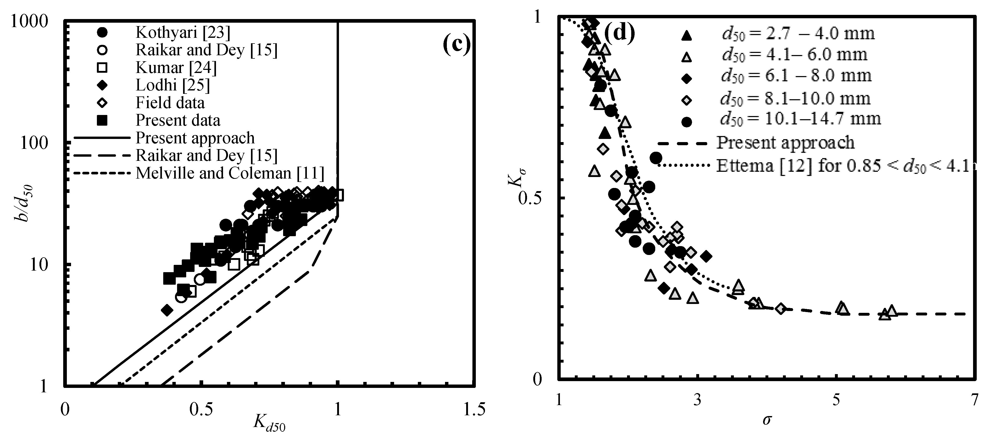
The gravel size factor Kd50 is defined as the influence of b* = b/d50 on d*se = dse/b. Melville and Coleman [11] stated that the decrease in the scour depth for comparatively coarser non-cohesive sediments was due to coarse particles obstructing the scour process near the pier and dissipating less flow energy in the scour region. Figure 4c illustrates the enveloping curve for Kd50 and shows that it can be governed by the following equations:
According to Melville and Coleman [11] and Raikar and Dey [15], the maximum equilibrium scour depth is independent of b* for b* ≥ 25, while in the present analysis, dse was found to be independent of b* for b* ≥ 35. However, in this experimental work, the whole scour area was typically roofed by the coarser size of gravel at an equilibrium scour condition. Therefore, the effect of the gravel size factor Kd50 could not be ignored.
3.2.4. Effect of Non-Uniformity Factor (Kσ)
Ettema [12] proposed a non-uniformity correction factor Kσ for uniform and non-uniform particles, as defined in Equation (6). The effect of Kσ as a function of the sediment gradation σ is shown in Figure 4d. According to Ettema [12], Kσ is constant for values of σ equal to or greater than 3.0; however, his study only considered values of σ from about 1.0 to 3.0. In this study, a wider range of σ from 1.41 to 5.8 was explored and it would appear that the value of the non-uniformity factor Kσ tended to be constant only for σ ≥ 3.8.
The maximum equilibrium scour depth dse in non-uniform gravel beds can be calculated in terms of the standard deviation of particle size distribution by using the values of Kσ. The non-uniform gravel size distribution has a significant effect on the maximum scour depth at the equilibrium stage: the sediment non-uniformity has been found to significantly reduce the scour processes [11].
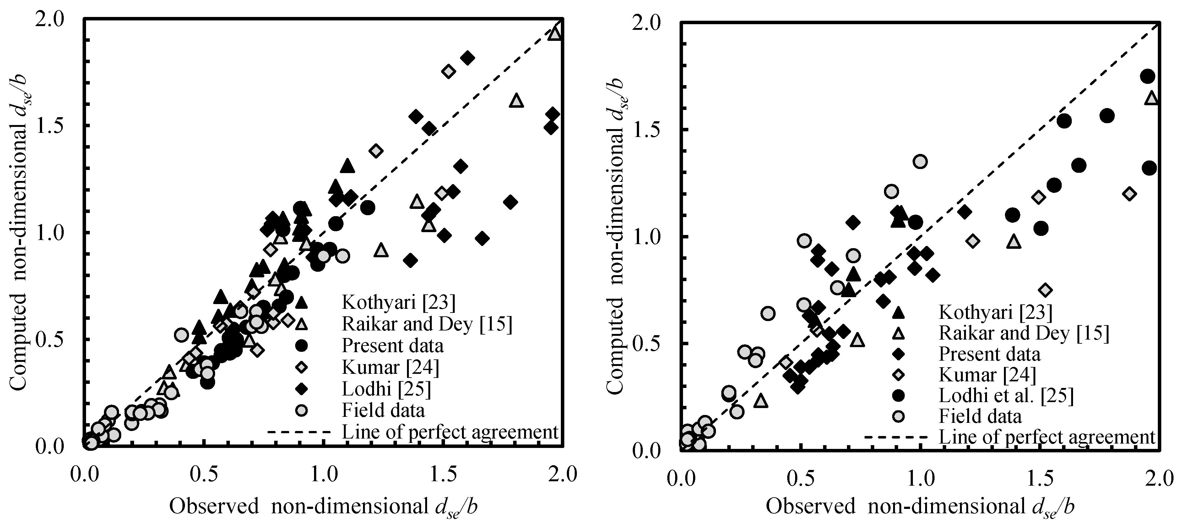
The calculation using the proposed model in Equation (9) showed a reasonably good accuracy when compared to various field and experimental datasets, as illustrated in Figure 5. By using the proposed K-factors, 80% of the datasets were found within the ±25% error margins at the calibration stage. Nearly 68% of the datasets were found within the ±25% error margins when considering all the data. The results still show good agreements at the validation stage (where 30% of the entire set of data was considered), with 75% of the datasets found to lie within the reasonable error limits, as presented in Figure 5.
3.3. Error and Statistical Calculations
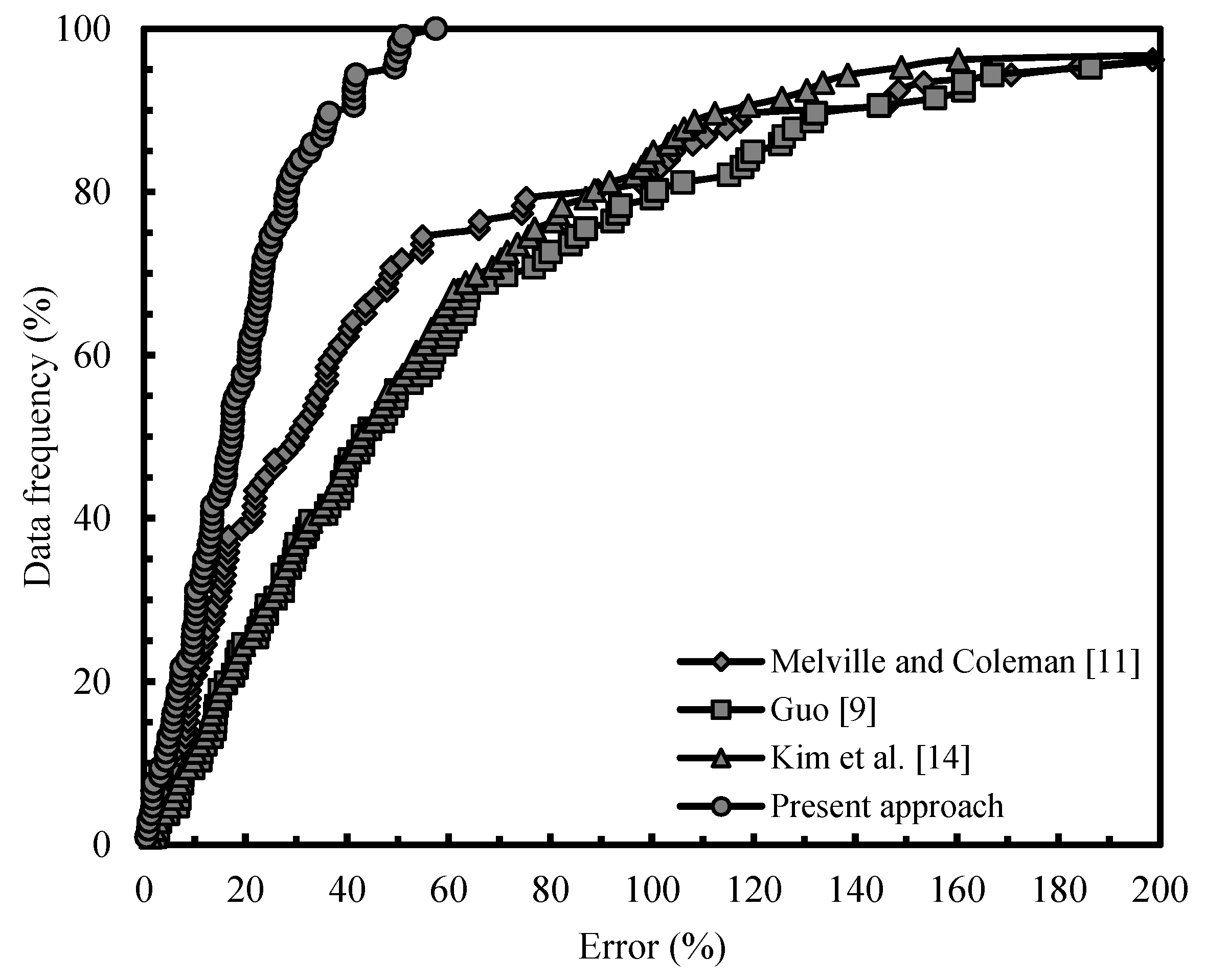
Figure 6 shows the calculated percentage error, which is the absolute value of the difference between the computed and experimental values of scour depth divided by the experimental value, against data frequency. By analyzing the previous Figure 3, it was recognized that the coarser laboratory data and the field data affected the accuracy of the considered literature approaches, which means that some datasets showed more than a 100% error (Figure 6). These errors were particularly high for Guo’s [9] and Kim et al.’s [14] approaches. Meanwhile, the equation given by Melville and Coleman [11] showed better agreements compared to the other two models. However, it was also necessary to make changes to Melville and Coleman’s [11] approach to estimate the maximum scour depth in coarser non-uniform riverbeds, as we have done in the new approach that was proposed and discussed in the previous sub-section. Figure 6 reveals that the proposed approach was capable of significantly reducing the percentage error for the coarser laboratory data and field data, hence providing a much better modeling accuracy for all the data.
More specifically, the percentage error and statistical indices were computed using the following formulae. These formulae depend on differences between the computed and experimental/field values of scour depths.
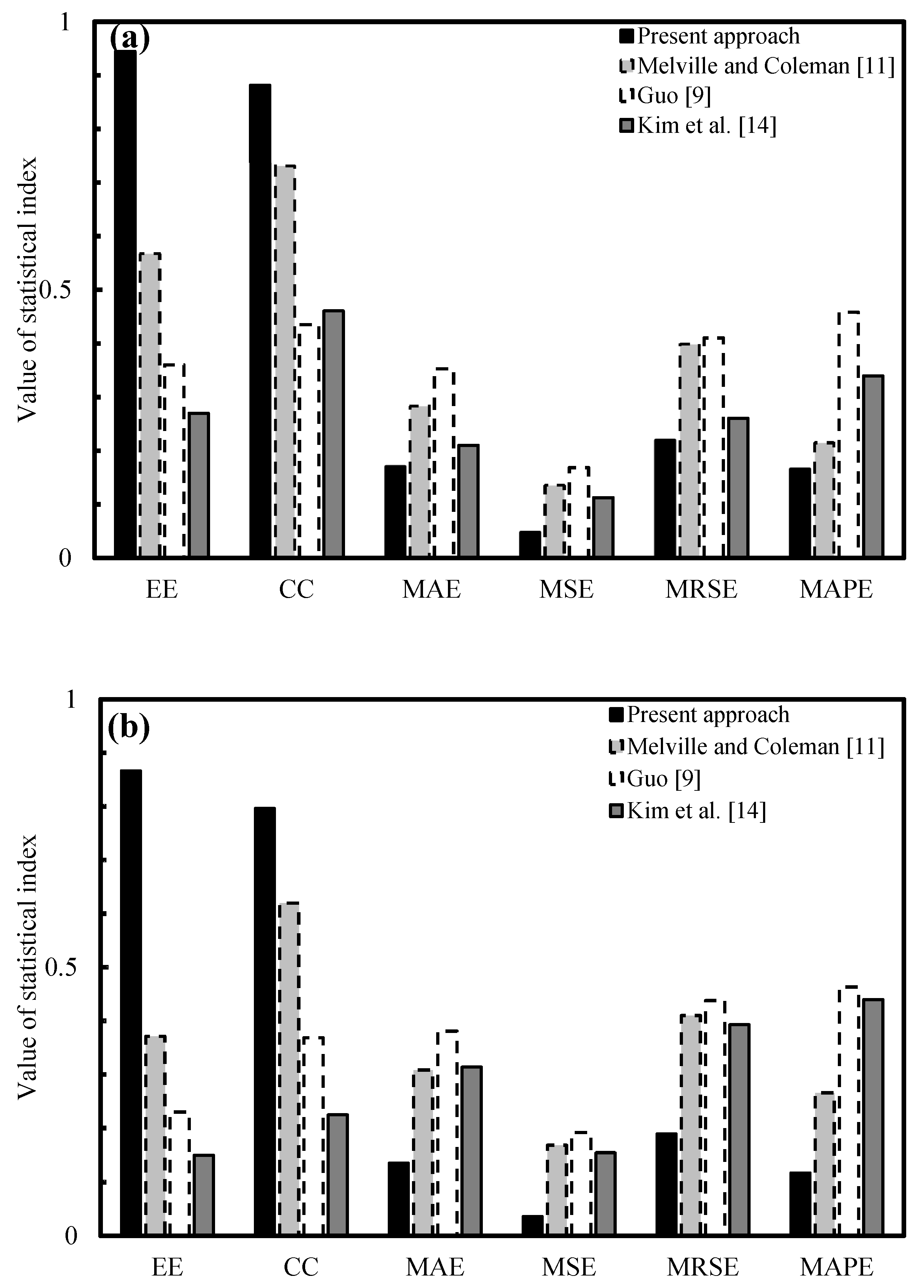
In Equations (13)–(18), is the observed maximum scour depth and is the computed maximum scour depth, n is the total number of maximum scour depth data (217 in the present study), CC is the coefficient of correlation, MAE is the mean absolute error, MSE is the mean squared error, MRSE is the mean root square error, and MAPE is the mean absolute percentage error. The values of these indices are presented in Figure 7. The values of CC and EE for the proposed approach were higher than the other approaches, and MAE, MSE, MRSE, and MAPE were lower for both the laboratory and field datasets. These statistical indices confirmed that the present approach performed significantly better than the literature approaches considered in this study. When focusing on the field datasets, both of the approaches used by Guo [9] and Kim et al. [14] showed similar performances but with unacceptable accuracies, while the approach from Melville and Coleman [11] showed better outcomes.
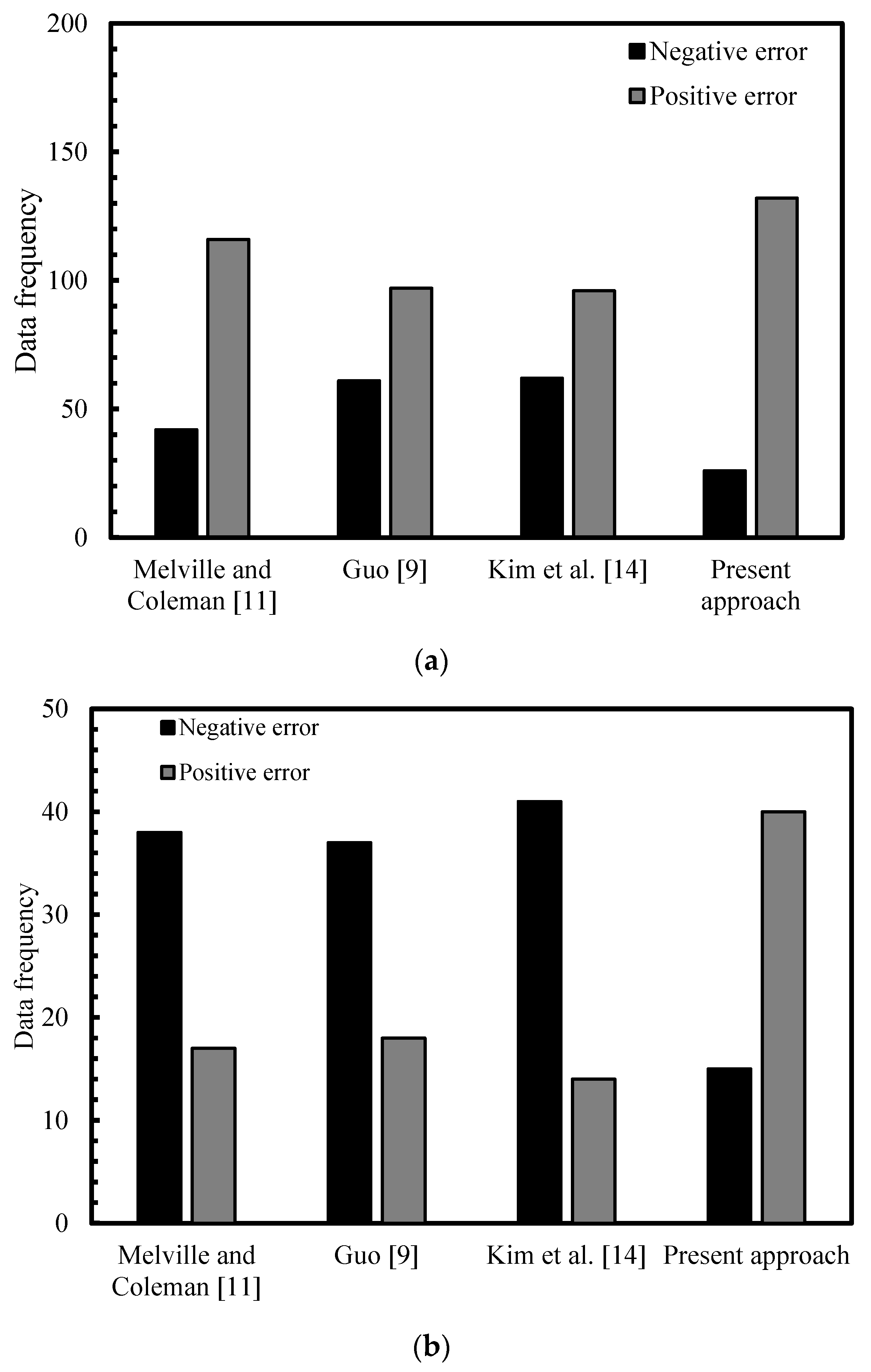
The distributions of positive and negative errors are shown in Figure 8 and Figure 9. The equations proposed by Guo [9] and Kim et al. [14] tended to underpredict the maximum scour depth. Conversely, the approach by Melville and Coleman [11] tended to slightly overpredict the maximum scour depth for the laboratory data and significantly overpredict the field data. The present approach consistently showed the best negative averaged error for both the laboratory and field datasets. For the laboratory datasets, the Melville and Coleman’s [11] approach and the proposed approach exhibited a comparable performance.
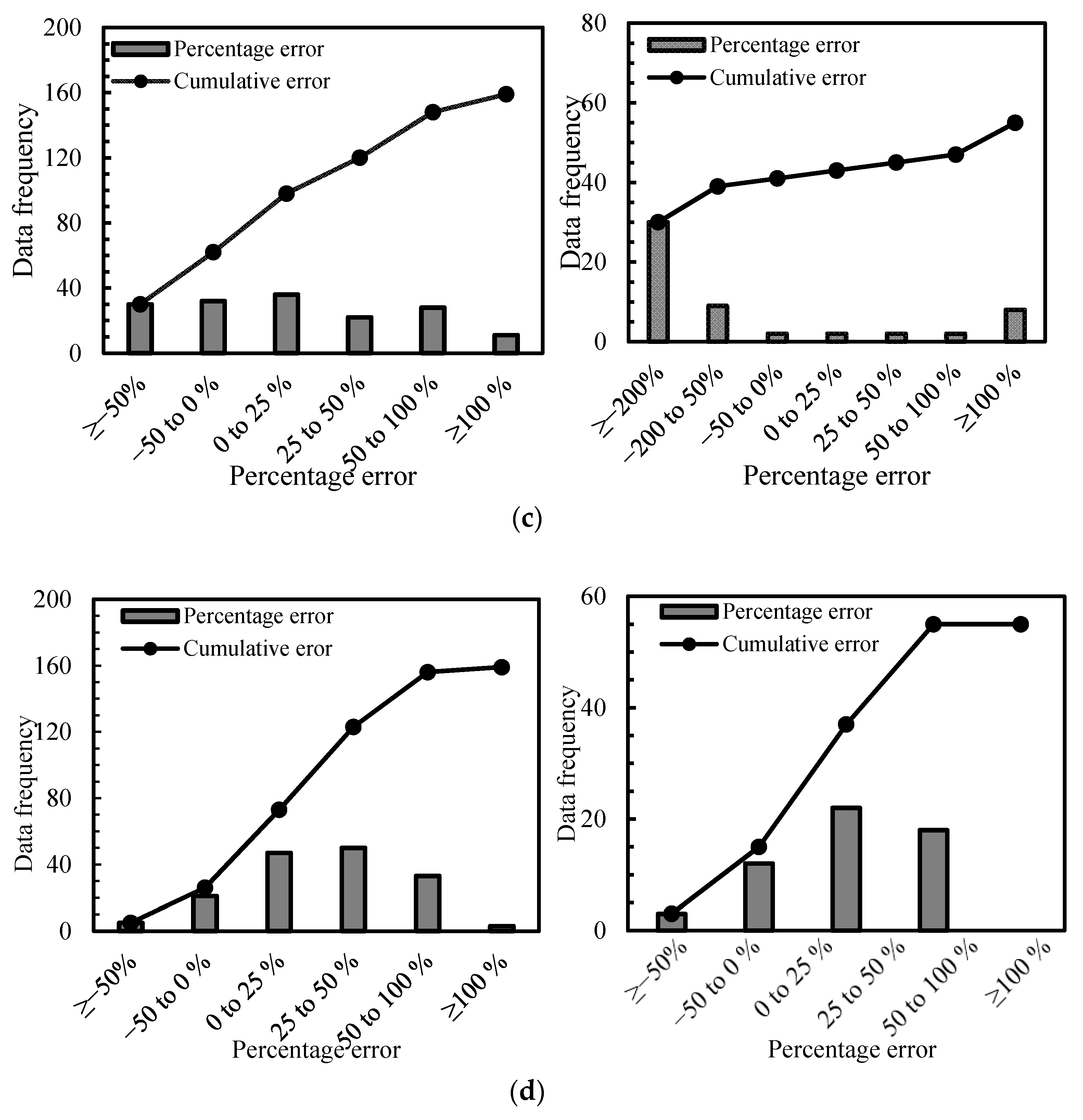
Figure 9a,b illustrate the histograms of the cumulative frequency for each error distribution using laboratory and field datasets for present and previous approaches. For the laboratory datasets, most of the percentage errors for the proposed approach were located at errors within 0–50%, while the percentage errors for the other approaches were typically located in the range between −50% and +50% (as shown in Figure 8 and Figure 9a). For the field datasets, most of the percentage errors for the present approach were located at errors within 25–100%, while the percentage errors for the other approaches were typically located between −200% and +25% (as shown in Figure 8 and Figure 9b). Overall, other literature approaches largely underpredict the maximum scour depth. Guo [9] and Kim et al. [14] show around 40% negative errors for laboratory datasets, while Melville and Coleman [11] show 25% negative errors. For field datasets, all previous studies show more than 65% negative errors. In comparison, for both the laboratory and field datasets, the present approach showed between only 15% and 30% negative errors, respectively. As summarized from Figure 8, the present approach produced small and positive errors compared to the previous approaches, which showed that the present approach performed well under both laboratory and field conditions.
3.4. Sensitivity Analysis
A sensitivity analysis was also performed to categorize the most critical K-factor, which influenced the scour depth calculations. This analysis was completed by taking the average values of all K-factors using the laboratory and field datasets. During the sensitivity analysis, an assumption was made stating that each K-factor was independent. The average values of Kby, KI, Kd50, and Kσ for the laboratory and field datasets were 0.89, 1.17, 0.84, and 0.34, respectively.
In terms of the sensitivity analysis methodology, if a percentage error ΔZ in the output is known as the difference between the values of output computed for inputs X and X + ΔX, then the percentage error can be estimated as the absolute sensitivity (A.S. = ΔZ/ΔX). Here, the output was X = dse and the input was X = Kby, KI, Kd50, and Kσ. The error ΔZ in the output is fundamentally the deviation sensitivity, with ΔX being the error. The relative sensitivity can be expressed as R.S. = (X × ΔZ)/(Z × ΔX) [36]. A linear sensitivity analysis was selected here, mainly because it is more understandable and computationally cheap while preserving true quantitative information about the linear influence of parameters.
The sensitivity analysis was done by changing each K-factor by ±10%. Table 3 illustrates the outcomes of the sensitivity analysis, where it can be seen that Kσ was the most sensitive K-factor, followed by Kby, Kd50, and lastly, KI. For a 10% increase in the K-factors, the absolute sensitivity (A.S.) of Kσ was nearly 12.8, 4.4, and 3.3 times that of KI, Kd50, and Kby, respectively. However, for a 10% reduction in each K-factor, the A.S. of Kσ was nearly 6.2, 3.8, and 2.8 times that of KI, Kd50, and Kb, respectively. Thus, it can be concluded that the proposed model significantly depended on Kσ compared to Kby, Kd50, and KI.
4. Conclusions
There is a remarkable scarcity of studies on pier scour in gravel-bed streams and major efforts are needed in this respect. Among the novelties of this study, there was a collection of 85 new experiments at the laboratory scale, all of which had a duration equal to or greater than 10 h. The data we collected, along with those from the literature, allowed for improving the Melville and Coleman’s [11] approach in the interpretation of both laboratory and field data, where this might be an attractive advancement in knowledge in overcoming scale effects. In this study, a new approach was developed to estimate the maximum scour depth at a circular pier in non-cohesive, non-uniform gravel beds. In the proposed approach, the pier scour depth depended on the interaction of flow properties, pier geometry, and sediment properties through different K-factors. The most noticeable findings from this work are summarized as follows.
Three previous models on the maximum scour depth were considered by checking their accuracy using a wide range of laboratory and field data. Statistically and graphically, it was observed that Melville and Coleman’s [11] approach performed relatively well for laboratory datasets, while it overestimated for field datasets. The approaches proposed by Guo [9] and Kim et al. [14] showed good agreements between observed and calculated values of scour depths, but only for laboratory datasets related to fine sediments. The effect of non-uniform gravel size on maximum scour depth around the pier was prominent. As a result, new K-factors that were significantly different from those suggested by Melville and Coleman [11] were estimated using a curve-fitting method. Finally, a new approach was developed based on the newly derived K-factors. This approach was also well validated by the 30% laboratory and field datasets. Furthermore, it performed better than the current literature approaches. A sensitivity analysis was also conducted for the newly proposed model. It was found that the factor Kσ was the most sensitive K-factor, followed by Kby, Kd50, and KI.
The proposed approach was applied to non-uniform gravel beds with sediment gradation σ ranging from 1.41 to 5.80, cylindrical piers, and approach flow conditions characterized by fully turbulent flow, a clear-water regime, Froude numbers from 0.21 to 0.75, and densimetric Froude numbers from 1.33 to 3.56. According to Oliveto and Marino [37], typical conditions of a clear-water regime (or low sediment transport) might be flows over floodplains (also during floods) and coarse-bed rivers, especially with natural vegetation. However, it is known that the maximum local clear-water scour depth is typically 10% larger than the maximum live-bed scour depth. Therefore, clear-water scour conditions could also be considered to approximately predict the local scour under live-bed conditions. Finally, the proposed approach referred to quasi-equilibrium conditions, neglecting the effect of time; however, in non-uniform gravel beds, equilibrium conditions are generally reached in a short time because the sediment non-uniformity aims to reduce the scour processes significantly.
Author Contributions
M.P. and P.K.S. conducted the experiments; M.P., G.O., and J.H.P. analyzed the data, applied the methodology, and validated this experimental study; G.O., J.H.P., and C.S.P.O. revised and edited the manuscript. All authors have read and agreed to the published version of the manuscript.
Funding
This research received no external funding.
Acknowledgments
The authors kindly acknowledge the staff of the Hydraulic Engineering Laboratory, Department of Civil Engineering, Indian Institute of Technology Roorkee, Uttarakhand 247667, India.
Conflicts of Interest
The authors declare no conflict of interest.
References
- Azamathulla, H.M.; Yusoff, M.A.M.; Hasan, Z.A. Scour below submerged skewed pipeline. J. Hydrol. 2014, 509, 615–620. [Google Scholar] [CrossRef]
- Qi, W.-G.; Gao, F.-P. Physical modeling of local scour development around a large-diameter monopile in combined waves and current. Coast. Eng. 2014, 83, 72–81. [Google Scholar] [CrossRef] [Green Version]
- Barbetta, S.; Camici, S.; Moramarco, T. A reappraisal of bridge piers scour vulnerability: A case study in the Upper Tiber River basin (central Italy). J. Flood Risk Manag. 2017, 10, 283–300. [Google Scholar] [CrossRef]
- Qi, M.; Li, J.; Chen, Q. Comparison of existing equations for local scour at bridge piers: Parameter influence and validation. Nat. Hazards 2016, 82, 2089–2105. [Google Scholar] [CrossRef]
- Qi, M.; Li, J.; Chen, Q. Applicability analysis of pier-scour equations in the field: Error analysis by rationalizing measurement data. J. Hydraul. Eng. ASCE 2018, 144, 04018050. [Google Scholar] [CrossRef]
- Decò, A.; Frangopol, D.M. Life-cycle risk assessment of spatially distributed aging bridges under seismic and traffic hazards. Earthq. Spectra 2013, 29, 127–153. [Google Scholar] [CrossRef]
- Brandimarte, L.; Paron, P.; Di Baldassarre, G. Bridge pier scour: A review of processes, measurements and estimates. Environ. Eng. Manag. J. 2012, 11, 975–989. [Google Scholar] [CrossRef]
- Richardson, E.V.; Davis, S.R. Evaluating Scour at Bridges—Hydraulic Engineering Circular No. 18; Report No. FHWA NHI 01-001; U.S. Department of Transportation, Federal Highway Administration: Washington, DC, USA, 2001.
- Guo, J. Pier scour in clear water for sediment mixtures. J. Hydraul. Res. 2012, 50, 18–27. [Google Scholar] [CrossRef]
- Pu, J.H.; Tait, S.; Guo, Y.; Huang, Y.; Hanmaiahgari, P.R. Dominant features in three-dimensional turbulence structure: Comparison of non-uniform accelerating and decelerating flows. Environ. Fluid Mech. 2018, 18, 395–416. [Google Scholar] [CrossRef] [Green Version]
- Melville, B.W.; Coleman, S.E. Bridge Scour; Water Resources Publications, LLC: Lone Tree, CO, USA, 2000. [Google Scholar]
- Ettema, R. Scour at Bridge Piers. Ph.D. Thesis, University of Auckland, Auckland, New Zealand, 1980. [Google Scholar]
- Coleman, S.E. Clearwater local scour at complex piers. J. Hydraul. Eng. ASCE 2005, 131, 330–334. [Google Scholar] [CrossRef]
- Kim, I.; Fard, M.Y.; Chattopadhyay, A. Investigation of a bridge pier scour prediction model for safe design and inspection. J. Bridge Eng. 2015, 20, 04014088. [Google Scholar] [CrossRef]
- Raikar, R.V.; Dey, S. Clear-water scour at bridge piers in fine and medium gravel beds. Can. J. Civ. Eng. 2005, 32, 775–781. [Google Scholar] [CrossRef]
- Kothyari, U.C.; Hager, W.H.; Oliveto, G. Generalized approach for clear-water scour at bridge foundation elements. J. Hydraul. Eng. ASCE 2007, 133, 1229–1240. [Google Scholar] [CrossRef]
- Jueyi, S.U.I.; Afzalimehr, H.; Samani, A.K.; Maherani, M. Clear-water scour around semi-elliptical abutments with armored beds. Int. J. Sediment Res. 2010, 25, 233–245. [Google Scholar]
- Abderrezzak, K.E.K.; Moran, A.D.; Mosselman, E.; Bouchard, J.P.; Habersack, H.; Aelbrecht, D. A physical, movable-bed model for non-uniform sediment transport, fluvial erosion and bank failure in rivers. J. Hydroenviron. Res. 2014, 8, 95–114. [Google Scholar] [CrossRef]
- Pournazeri, S.; Li, S.S.; Haghighat, F. A bridge pier scour model with non-uniform sediments. Proc. Inst. Civ. Eng. Water Manag. 2012, 167, 499–511. [Google Scholar] [CrossRef]
- Sharma, A.; Chavan, R.; Kumar, B. Multi-scale statistical characterization of migrating pier scour depth in non-uniform sand bed channel. Int. J. River Basin Manag. 2017, 15, 265–276. [Google Scholar] [CrossRef]
- Pandey, M.; Chen, S.C.; Sharma, P.K.; Ojha, C.S.P.; Kumar, V. Local Scour of Armor Layer Processes around the Circular Pier in Non-Uniform Gravel Bed. Water 2019, 11, 1421. [Google Scholar] [CrossRef] [Green Version]
- Pandey, M.; Valyrakis, M.; Qi, M.; Sharma, A.; Lodhi, A.S. Experimental assessment and prediction of temporal scour depth around a spur dike. Int. J. Sediment Res. 2020, 1–10. [Google Scholar] [CrossRef]
- Kothyari, U.C. Scour around Bridge Piers. Ph.D. Thesis, Indian Institute of Technology Roorkee, Roorkee, India, 1989. [Google Scholar]
- Kumar, A. Scour around Circular Compound Bridge Piers. Ph.D. Thesis, Indian Institute of Technology Roorkee, Roorkee, India, 2007. [Google Scholar]
- Lodhi, A.S. Scour around Spur Dikes and Bridge Piers Founded in Cohesive Sediment Mixtures. Ph.D. Thesis, Indian Institute of Technology Roorkee, Roorkee, India, 2015. [Google Scholar]
- Benedict, S.T.; Caldwell, A.W. A Pier-Scour Database: 2427 Field and Laboratory Measurements of Pier Scour; U.S. Department of the Interior, U.S. Geological Survey: Reston, VA, USA, 2014.
- Pu, J.H.; Lim, S.Y. Efficient numerical computation and experimental study of temporally long equilibrium scour development around abutment. Environ. Fluid Mech. 2014, 14, 69–86. [Google Scholar] [CrossRef] [Green Version]
- Kothyari, U.C.; Ranga Raju, K.G. Scour around spur dikes and bridge abutments. J. Hydraul. Res. 2001, 39, 367–374. [Google Scholar] [CrossRef]
- Pandey, M.; Sharma, P.K.; Ahmad, Z.; Karna, N. Maximum scour depth around bridge pier in gravel bed streams. Nat. Hazards 2018, 91, 819–836. [Google Scholar] [CrossRef]
- Oliveto, G.; Hager, W.H. Temporal evolution of clear-water pier and abutment scour. J. Hydraul. Eng. ASCE 2002, 128, 811–820. [Google Scholar] [CrossRef]
- Graf, W.H.; Altinakar, M.S. Fluvial Hydraulics—Flow and Transport Processes in Channels of Simple Geometry; John Wiley & Sons Ltd.: Chichester, UK, 1998; pp. 10–12. [Google Scholar]
- Ballio, F.; Teruzzi, A.; Radice, A. Constriction effects in clear-water scour at abutments. J. Hydraul. Eng. ASCE 2009, 135, 140–145. [Google Scholar] [CrossRef]
- Melville, B.W.; Sutherland, A.J. Design method for local scour at bridge piers. J. Hydraul. Eng. ASCE 1988, 114, 1210–1226. [Google Scholar] [CrossRef]
- Chiew, Y.M. Local Scour at Bridge Piers. Ph.D. Thesis, University of Auckland, Auckland, New Zealand, 1984. [Google Scholar]
- Baker, R.E. Local Scour at Bridge Piers in Non Uniform Sediment. Master’s of Philosophy Thesis, University of Auckland, Auckland, New Zealand, 1986. [Google Scholar]
- Pandey, M.; Lam, W.H.; Cui, Y.; Khan, M.A.; Singh, U.K.; Ahmad, Z. Scour around Spur Dike in Sand–Gravel Mixture Bed. Water 2019, 11, 1417. [Google Scholar] [CrossRef] [Green Version]
- Oliveto, G.; Marino, M.C. Temporal scour evolution at non-uniform bridge piers. Proc. Inst. Civ. Eng. Water Manag. 2017, 170, 254–261. [Google Scholar] [CrossRef]
Figure 1.
Bridge on a gravel-and-cobble-bed stream in Calabria, Southern Italy. The view is from upstream to downstream.
Figure 1.
Bridge on a gravel-and-cobble-bed stream in Calabria, Southern Italy. The view is from upstream to downstream.

Figure 2.
Layout of the experimental setup used in this study.

Figure 3.
Calculated vs. observed non-dimensional scour depths using (a) Melville and Coleman’s [11], (b) Guo’s [9], and (c) Kim et al.’s [14] approaches.

Figure 4.
(a) Enveloping curve between d*se and y*, (b) enveloping curve found when computing KI, (c) enveloping curve found when computing Kd50, and (d) effect of non-uniformity factor Kσ on σ.
Figure 4.
(a) Enveloping curve between d*se and y*, (b) enveloping curve found when computing KI, (c) enveloping curve found when computing Kd50, and (d) effect of non-uniformity factor Kσ on σ.


Figure 5.
Calculated vs. observed non-dimensional scour depth using the present approach. The plot on the left refers to the 70% of the entire set of data used for calibration and the plot on the right refers to the remaining 30% of data used for validation.
Figure 5.
Calculated vs. observed non-dimensional scour depth using the present approach. The plot on the left refers to the 70% of the entire set of data used for calibration and the plot on the right refers to the remaining 30% of data used for validation.

Figure 6.
Percentage errors in estimates of the scour depth against data frequency using the present and previous pier scour approaches.
Figure 6.
Percentage errors in estimates of the scour depth against data frequency using the present and previous pier scour approaches.

Figure 7.
Variation of different statistical indices using (a) laboratory data and (b) field data (all statistical indices are dimensionless).
Figure 7.
Variation of different statistical indices using (a) laboratory data and (b) field data (all statistical indices are dimensionless).

Figure 8.
Error distributions using laboratory data (left column) and field data (right column): (a) Melville and Coleman [11], (b) Guo [9], (c) Kim et al. [14], and (d) the present approach.


Figure 9.
Positive and negative error distributions using (a) laboratory experimental data and (b) field data.
Figure 9.
Positive and negative error distributions using (a) laboratory experimental data and (b) field data.


Table 1.
Main conditions and outcomes for the experiments from literature sources.
| Literature Source | Data Type | y (m) | U (m/s) | b (m) | d50 (mm) | σ | U/Uc |
|---|---|---|---|---|---|---|---|
| Raikar and Dey [15] | Lab | 0.25 | 0.76–1.10 | 0.03–0.08 | 4.10–14.25 | 1.43–2.90 | 0.66–0.96 |
| Kothyari [23] | Lab | 0.06–0.13 | 0.25–0.31 | 0.05–0.11 | 8.30 | 1.80 | 0.70–0.95 |
| Kumar [24] | Lab | 0.16–0.19 | 0.28–0.44 | 0.05–0.20 | 3.47–4.00 | 1.52–1.67 | 0.54–0.86 |
| Lodhi [25] | Lab | 0.08–0.25 | 0.30–1.10 | 0.08–0.12 | 2.70–5.53 | 1.43–1.51 | 0.60–0.95 |
| Benedict and Caldwell [26] | Field | 0.91–5.58 | 0.95–3.66 | 0.76–1.52 | 2.70–6.10 | 1.50–5.80 | 0.52–0.89 |
Table 2.
Main conditions and outcomes for the experiments carried out in this study.
| Run | b (m) | d50 (m) | σ | y (m) | U (m/s) | U/Uc | dse (m) | te (h) | t* (h) |
|---|---|---|---|---|---|---|---|---|---|
| R1 | 0.066 | 0.00494 | 1.51 | 0.14 | 0.61 | 0.938 | 0.042 | 10 | 11.24 |
| R2 | 0.066 | 0.00494 | 1.51 | 0.13 | 0.55 | 0.846 | 0.035 | 12 | 10.98 |
| R3 | 0.066 | 0.00494 | 1.51 | 0.10 | 0.46 | 0.708 | 0.026 | 15 | 9.70 |
| R4 | 0.084 | 0.00494 | 1.51 | 0.14 | 0.61 | 0.938 | 0.071 | 11 | 10.28 |
| R5 | 0.084 | 0.00494 | 1.51 | 0.13 | 0.55 | 0.846 | 0.062 | 11 | 9.69 |
| R6 | 0.084 | 0.00494 | 1.51 | 0.10 | 0.46 | 0.708 | 0.032 | 14 | 11.06 |
| R7 | 0.115 | 0.00494 | 1.51 | 0.14 | 0.61 | 0.938 | 0.118 | 10 | 9.73 |
| R8 | 0.115 | 0.00494 | 1.51 | 0.13 | 0.55 | 0.846 | 0.111 | 12 | 11.04 |
| R9 | 0.115 | 0.00494 | 1.51 | 0.10 | 0.46 | 0.708 | 0.082 | 15 | 9.51 |
| R10 | 0.135 | 0.00494 | 1.51 | 0.14 | 0.61 | 0.938 | 0.160 | 11 | 8.66 |
| R11 | 0.135 | 0.00494 | 1.51 | 0.13 | 0.55 | 0.846 | 0.136 | 14 | 8.27 |
| R12 | 0.135 | 0.00494 | 1.51 | 0.10 | 0.46 | 0.708 | 0.089 | 15 | 8.25 |
| R13 | 0.066 | 0.00438 | 1.88 | 0.14 | 0.61 | 0.984 | 0.050 | 11 | 9.79 |
| R14 | 0.066 | 0.00438 | 1.88 | 0.13 | 0.58 | 0.935 | 0.042 | 12 | 10.04 |
| R15 | 0.066 | 0.00438 | 1.88 | 0.10 | 0.53 | 0.855 | 0.031 | 14 | 9.68 |
| R16 | 0.084 | 0.00438 | 1.88 | 0.14 | 0.61 | 0.984 | 0.082 | 10 | 8.86 |
| R17 | 0.084 | 0.00438 | 1.88 | 0.13 | 0.58 | 0.935 | 0.079 | 12 | 8.16 |
| R18 | 0.084 | 0.00438 | 1.88 | 0.10 | 0.53 | 0.855 | 0.062 | 15 | 7.62 |
| R19 | 0.115 | 0.00438 | 1.88 | 0.14 | 0.61 | 0.984 | 0.112 | 11 | 9.93 |
| R20 | 0.115 | 0.00438 | 1.88 | 0.13 | 0.58 | 0.935 | 0.101 | 12 | 9.72 |
| R21 | 0.115 | 0.00438 | 1.88 | 0.10 | 0.53 | 0.855 | 0.068 | 14 | 10.41 |
| R22 | 0.135 | 0.00438 | 1.88 | 0.14 | 0.61 | 0.984 | 0.142 | 14 | 9.64 |
| R23 | 0.135 | 0.00438 | 1.88 | 0.13 | 0.58 | 0.935 | 0.132 | 15 | 9.11 |
| R24 | 0.135 | 0.00438 | 1.88 | 0.10 | 0.53 | 0.855 | 0.078 | 13 | 10.80 |
| R25 | 0.066 | 0.00382 | 1.71 | 0.13 | 0.55 | 0.932 | 0.040 | 12 | 12.18 |
| R26 | 0.066 | 0.00382 | 1.71 | 0.12 | 0.49 | 0.831 | 0.031 | 14 | 12.26 |
| R27 | 0.066 | 0.00382 | 1.71 | 0.11 | 0.45 | 0.763 | 0.015 | 15 | 13.52 |
| R28 | 0.084 | 0.00382 | 1.71 | 0.13 | 0.55 | 0.932 | 0.052 | 12 | 13.44 |
| R29 | 0.084 | 0.00382 | 1.71 | 0.12 | 0.49 | 0.831 | 0.046 | 14 | 12.43 |
| R30 | 0.084 | 0.00382 | 1.71 | 0.11 | 0.45 | 0.763 | 0.029 | 16 | 14.56 |
| R31 | 0.115 | 0.00382 | 1.71 | 0.13 | 0.55 | 0.932 | 0.096 | 13 | 12.29 |
| R32 | 0.115 | 0.00382 | 1.71 | 0.12 | 0.49 | 0.831 | 0.060 | 15 | 14.75 |
| R33 | 0.115 | 0.00382 | 1.71 | 0.11 | 0.45 | 0.763 | 0.023 | 15 | 18.16 |
| R34 | 0.135 | 0.00382 | 1.71 | 0.13 | 0.55 | 0.932 | 0.112 | 12 | 13.11 |
| R35 | 0.135 | 0.00382 | 1.71 | 0.12 | 0.49 | 0.831 | 0.081 | 14 | 14.19 |
| R36 | 0.135 | 0.00382 | 1.71 | 0.11 | 0.45 | 0.763 | 0.049 | 15 | 17.65 |
| R37 | 0.066 | 0.00326 | 1.59 | 0.13 | 0.53 | 0.946 | 0.041 | 12 | 13.97 |
| R38 | 0.066 | 0.00326 | 1.59 | 0.12 | 0.48 | 0.857 | 0.036 | 14 | 13.25 |
| R39 | 0.066 | 0.00326 | 1.59 | 0.105 | 0.44 | 0.786 | 0.025 | 14 | 14.10 |
| R40 | 0.084 | 0.00326 | 1.59 | 0.13 | 0.54 | 0.964 | 0.073 | 12 | 12.73 |
| R41 | 0.084 | 0.00326 | 1.59 | 0.12 | 0.48 | 0.857 | 0.063 | 15 | 11.88 |
| R42 | 0.084 | 0.00326 | 1.59 | 0.105 | 0.44 | 0.786 | 0.035 | 14 | 15.01 |
| R43 | 0.115 | 0.00326 | 1.59 | 0.13 | 0.54 | 0.964 | 0.104 | 15 | 14.01 |
| R44 | 0.135 | 0.00326 | 1.59 | 0.13 | 0.54 | 0.964 | 0.122 | 15 | 14.90 |
| R45 | 0.135 | 0.01070 | 1.57 | 0.125 | 0.79 | 0.898 | 0.081 | 11 | 9.37 |
| R46 | 0.135 | 0.01070 | 1.57 | 0.125 | 0.76 | 0.864 | 0.072 | 11 | 9.80 |
| R47 | 0.135 | 0.01070 | 1.57 | 0.125 | 0.74 | 0.841 | 0.064 | 12 | 10.38 |
| R48 | 0.115 | 0.01070 | 1.57 | 0.125 | 0.79 | 0.898 | 0.070 | 10 | 8.67 |
| R49 | 0.115 | 0.01070 | 1.57 | 0.125 | 0.76 | 0.864 | 0.063 | 12 | 8.99 |
| R50 | 0.115 | 0.01070 | 1.57 | 0.125 | 0.74 | 0.841 | 0.051 | 12 | 10.12 |
| R51 | 0.084 | 0.01070 | 1.57 | 0.125 | 0.79 | 0.898 | 0.053 | 11 | 7.40 |
| R52 | 0.084 | 0.01070 | 1.57 | 0.125 | 0.76 | 0.864 | 0.045 | 10 | 7.97 |
| R53 | 0.084 | 0.01070 | 1.57 | 0.125 | 0.74 | 0.841 | 0.040 | 12 | 8.39 |
| R54 | 0.066 | 0.01070 | 1.57 | 0.125 | 0.79 | 0.898 | 0.034 | 10 | 7.60 |
| R55 | 0.066 | 0.01070 | 1.57 | 0.125 | 0.76 | 0.864 | 0.031 | 11 | 7.75 |
| R56 | 0.066 | 0.01070 | 1.57 | 0.125 | 0.74 | 0.841 | 0.022 | 11 | 9.13 |
| R57 | 0.115 | 0.00910 | 1.66 | 0.13 | 0.76 | 0.974 | 0.073 | 13 | 8.52 |
| R58 | 0.115 | 0.00910 | 1.66 | 0.13 | 0.74 | 0.949 | 0.069 | 12 | 8.63 |
| R59 | 0.115 | 0.00910 | 1.66 | 0.13 | 0.72 | 0.923 | 0.065 | 14 | 8.75 |
| R60 | 0.135 | 0.00910 | 1.66 | 0.13 | 0.74 | 0.949 | 0.110 | 13 | 6.88 |
| R61 | 0.135 | 0.00910 | 1.66 | 0.13 | 0.74 | 0.949 | 0.091 | 12 | 8.31 |
| R62 | 0.135 | 0.00860 | 1.63 | 0.13 | 0.74 | 0.974 | 0.097 | 12 | 8.71 |
| R63 | 0.135 | 0.00860 | 1.63 | 0.13 | 0.72 | 0.947 | 0.085 | 12 | 9.43 |
| R64 | 0.135 | 0.00860 | 1.63 | 0.13 | 0.70 | 0.921 | 0.077 | 13 | 9.88 |
| R65 | 0.115 | 0.00860 | 1.63 | 0.13 | 0.74 | 0.974 | 0.066 | 12 | 9.80 |
| R66 | 0.115 | 0.00860 | 1.63 | 0.13 | 0.70 | 0.921 | 0.056 | 13 | 10.38 |
| R67 | 0.115 | 0.00860 | 1.63 | 0.13 | 0.70 | 0.921 | 0.066 | 12 | 9.43 |
| R68 | 0.084 | 0.00860 | 1.63 | 0.13 | 0.74 | 0.974 | 0.045 | 10 | 8.95 |
| R69 | 0.084 | 0.00860 | 1.63 | 0.13 | 0.72 | 0.947 | 0.042 | 12 | 9.11 |
| R70 | 0.084 | 0.00860 | 1.63 | 0.13 | 0.70 | 0.921 | 0.039 | 13 | 9.30 |
| R71 | 0.066 | 0.00860 | 1.63 | 0.13 | 0.74 | 0.974 | 0.030 | 11 | 8.82 |
| R72 | 0.066 | 0.00860 | 1.63 | 0.13 | 0.72 | 0.947 | 0.025 | 12 | 9.52 |
| R73 | 0.066 | 0.00860 | 1.63 | 0.13 | 0.70 | 0.921 | 0.018 | 12 | 10.92 |
| R74 | 0.135 | 0.00750 | 1.56 | 0.13 | 0.73 | 0.973 | 0.101 | 10 | 9.87 |
| R75 | 0.135 | 0.00750 | 1.56 | 0.13 | 0.71 | 0.947 | 0.092 | 12 | 10.31 |
| R76 | 0.135 | 0.00750 | 1.56 | 0.13 | 0.69 | 0.920 | 0.084 | 14 | 10.72 |
| R77 | 0.115 | 0.00750 | 1.56 | 0.13 | 0.73 | 0.973 | 0.078 | 11 | 10.03 |
| R78 | 0.115 | 0.00750 | 1.56 | 0.13 | 0.71 | 0.947 | 0.069 | 12 | 10.65 |
| R79 | 0.115 | 0.00750 | 1.56 | 0.13 | 0.69 | 0.920 | 0.063 | 12 | 11.02 |
| R80 | 0.084 | 0.00750 | 1.56 | 0.13 | 0.73 | 0.973 | 0.048 | 12 | 9.85 |
| R81 | 0.084 | 0.00750 | 1.56 | 0.13 | 0.71 | 0.947 | 0.045 | 11 | 10.00 |
| R82 | 0.084 | 0.00750 | 1.56 | 0.13 | 0.69 | 0.920 | 0.044 | 11 | 9.87 |
| R83 | 0.066 | 0.00750 | 1.56 | 0.13 | 0.73 | 0.973 | 0.033 | 11 | 9.52 |
| R84 | 0.066 | 0.00750 | 1.56 | 0.13 | 0.71 | 0.947 | 0.037 | 12 | 8.70 |
| R85 | 0.066 | 0.00750 | 1.56 | 0.13 | 0.69 | 0.920 | 0.031 | 12 | 9.41 |
Table 3.
Sensitivity analysis with a 10% increment or reduction in K-factors.
| Percentage Change | X | ΔX | ΔZ | A.S. | R.S. |
|---|---|---|---|---|---|
| 10% increment | Kσ | 0.034 | 0.057 | 1.66 | 2.67 |
| Kby | 0.089 | 0.046 | 0.51 | 2.17 | |
| Kd50 | 0.084 | 0.032 | 0.38 | 1.51 | |
| KI | 0.117 | 0.015 | 0.13 | 0.69 | |
| 10% reduction | Kσ | 0.034 | −0.041 | −1.18 | −1.92 |
| Kby | 0.089 | −0.037 | −0.42 | −1.78 | |
| Kd50 | 0.084 | −0.025 | −0.31 | −1.21 | |
| KI | 0.117 | −0.022 | −0.19 | −1.06 |
© 2020 by the authors. Licensee MDPI, Basel, Switzerland. This article is an open access article distributed under the terms and conditions of the Creative Commons Attribution (CC BY) license (http://creativecommons.org/licenses/by/4.0/).
Share and Cite
MDPI and ACS Style
Pandey, M.; Oliveto, G.; Pu, J.H.; Sharma, P.K.; Ojha, C.S.P. Pier Scour Prediction in Non-Uniform Gravel Beds. Water 2020, 12, 1696. https://doi.org/10.3390/w12061696
AMA Style
Pandey M, Oliveto G, Pu JH, Sharma PK, Ojha CSP. Pier Scour Prediction in Non-Uniform Gravel Beds. Water. 2020; 12(6):1696. https://doi.org/10.3390/w12061696
Chicago/Turabian StylePandey, Manish, Giuseppe Oliveto, Jaan H. Pu, P. K. Sharma, and C. S. P. Ojha. 2020. "Pier Scour Prediction in Non-Uniform Gravel Beds" Water 12, no. 6: 1696. https://doi.org/10.3390/w12061696
Note that from the first issue of 2016, this journal uses article numbers instead of page numbers. See further details here.