Design and Bench-Scale Hydrodynamic Testing of Thin-Layer Wavy Photobioreactors


1
Department of Civil and Environmental Engineering, Sapienza Università di Roma, Via Eudossiana 18, 00184 Rome, Italy
2
Department of Chemical Engineering, Sapienza Università di Roma, Via Eudossiana 18, 00184 Rome, Italy
3
Bio-P s.r.l., via di Vannina 88, 00156 Rome, Italy
*
Author to whom correspondence should be addressed.
Water 2019, 11(7), 1521; https://doi.org/10.3390/w11071521
Submission received: 12 June 2019
/
Revised: 12 July 2019
/
Accepted: 19 July 2019
/
Published: 23 July 2019
(This article belongs to the Special Issue Integration of Microalgal Based Processes in Wastewater Treatment)
Abstract
:In a thin-volume photobioreactor where a concentrated suspension of microalgae is circulated throughout the established spatial irradiance gradient, microalgal cells experience a time-variable irradiance. Deploying this feature is the most convenient way of obtaining the so-called “flashing light” effect, improving biomass production in high irradiance. This work investigates the light flashing features of sloping wavy photobioreactors, a recently proposed type, by introducing and validating a computational fluid dynamics (CFD) model. Two characteristic flow zones (straight top-to-bottom stream and local recirculation stream), both effective toward light flashing, have been found and characterized: a recirculation-induced frequency of 3.7 Hz and straight flow-induced frequency of 5.6 Hz were estimated. If the channel slope is increased, the recirculation area becomes less stable while the recirculation frequency is nearly constant with flow rate. The validated CFD model is a mighty tool that could be reliably used to further increase the flashing frequency by optimizing the design, dimensions, installation, and operational parameters of the sloping wavy photobioreactor.
1. Introduction
Microalgae are considered as one of the most promising fast-growing photosynthetic microorganisms on Earth; hence, it is expected that they can play an important role in CO2 sequestration, food, feed, sourcing of biochemical products, commodities, biofuels, and phytodepuration.
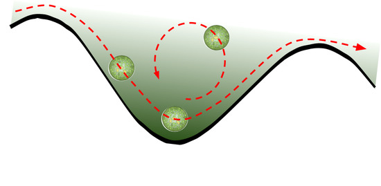
Due to significant light attenuation along the light path [1], concentrated microalgal suspensions need to be cultured at minimal thickness to avoid reducing the volume-based specific growth rate [2] so cells that circulate back and forth along the established spatially distributed irradiance gradient experience a time-varying irradiance, which is the flashing light effect. The “flashing light” effect is extremely beneficial in outdoor cultures because microalgae reach their maximum photosynthetic activity at roughly 1/10 of the maximum irradiation recorded in summer days, and photosynthetic machinery is damaged by photooxidation and photoinhibition well below the maximum sunlight irradiance values [3] if light is not alternated with darkness at a proper rate. Indeed, the combination between an excessively large dark volume and an excessive irradiance in the well-illuminated zone is the main cause that limits the productivity of established commercial photobioreactors (PBRs) to one order of magnitude below the theoretical limit. This depression would be partly offset if cells were exposed to a rapidly variable irradiance as an effect of hydrodynamically travelling across differently lit zones.
Apparently, there is quite substantial discrepancy among the quantitative estimates of the benefits of light flashing, and this is at least partly due to differences in the experimental setup or assumptions concerning the operational mode of the equipment used to carry out the experimental investigation, such as the irradiance spectrum, the operational dark volume fraction of the photobioreactor, and the culturing mode. As an example of the different conclusions that may be drawn from the recent literature, it was observed that photosynthetic rates increase exponentially with an increasing light-to-darkness (L/D) frequency, and they also depend upon: (1) the L/D ratio, (2) the light acclimation state of the culture (low or high irradiance), and (3) the light intensity exposition history [4]. However, L/D cycles of 1 and 10 Hz were found to result in a 10% lower biomass yield than in continuous light (therefore, a growth depression), while L/D cycles of 100 Hz resulted in a 35% boost of biomass productivity [5]. Low-frequency, hydrodynamically induced light pulsation was found to increase productivity by 38%–48% (depending on the cultured species) in an airlift photobioreactor featuring spatial alternation of irradiation rates creating a light pulse frequency of 10 Hz [6]. On the other hand, a significant penalty occurs when L/D alternation is in the range ~0.1 to ~0.01 Hz under short lighting duty cycles and during purely autotrophic growth [7]. An important point that motivates intricacy in the analysis of flashing light experimental data, and the consequent assessment of the growth promotion claim, resides in the difference between the specific observed growth rate of a cell population exposed to a spatially uniform, time-varying irradiance, and that of a cell population of such density to completely absorb the impinging irradiance over the culture thickness. Complete absorption, indeed, maximizes light utilization by the culture and, thus, also maximizes areal productivity [2,8]. Mass transfer efficiency in mass-transfer-limited cultures is synergic with photosynthetic activity promotion; since concentrated cultures may be mass transfer limited, care must be exerted both in designing experiments aimed at quantifying the effects of light flashing of hydrodynamic origin and in subsequent data analyses [9]. Finally, it has been underlined that L/D cycles with a well-defined frequency result in enhancing productivity more than chaotic L/D alternation [10].
The ways to induce fast alternation of illumination and darkness perceived by the microalgal cells beyond the slow (day/night) cycle, which microalgae are normally exposed to, include: (i) flashing artificial illumination [11] and (ii) hydrodynamic displacement of cells entrained in the medium experiencing differently lit zones, while the photobioreactor exposed surface is subjected to a stationary radiative field [12]. In this latter case, perceived flashing is the result of the combined effect of the photobioreactor’s geometry, of the adopted circulation flow, and of the microalgal culture characteristics (viscosity and optical density). In the case of mixing-induced L/D cycles, it has been noted that algal productivity increases as the Reynolds number is increased [13]. However, high recirculation rates may depress productivity, and operation of the photobioreactor may require an excessive energy input [14]. Increased turbulence also enhances the exchange rates of nutrients and metabolites between the cells and their growth medium [15]. To achieve a hydrodynamically induced flashing, Torzillo and others developed a novel photobioreactor design featuring a sloping, wavy-bottomed surface [16], which differs from the uniform thin-layer cascade system with a flat bottom designed by Setlik and others [17]. When installed with a low inclination angle, this photobioreactor features a spatial alternation of deep (wave troughs) and shallow (wave ridges) zones. Compared to many conventional culture systems, this photobioreactor design: (1) features an optically thin culture that is amenable to high cell concentrations, which is amongst the top requirements for lowering biomass harvest costs [16]; (2) provides an efficient gas–liquid mass transfer, with a positive dependence upon specific flow rate [15]; (3) features a low equipment cost (can be produced from low-cost, semi-finished materials); and (4) has hydrodynamic features leading to regular, specific flow rate dependent L/D alternation, which might result in increased photosynthetic activity with respect to other frequently adopted (e.g., tubular and bubble column) photobioreactor geometries. It was shown that in a 15-cavity wavy-bottomed lower surface photobioreactor, a local recirculation zone was established in each cavity only at low inclinations (≤6°), and its location changed according to the inclination slope from the lower (0° and 3°) to the upper part of each cavity (6°) [18]. Sforza and others have warned that the combination between species, external irradiance, and hydrodynamic mixing frequency must be carefully checked before investing in a specific photobioreactor installation [19]. The burden of experimentally investigating a variety of design and operational photobioreactor alternatives [19] motivates the development and validation of a computational fluid dynamics (CFD) model. By such a model, further development of the sloping wavy-bottom photobioreactor can be fostered, as reported for other novel photobioreactors [20,21,22]. Development of such a CFD model is the object of the present work. Indeed, the present work provides, at one time, a description of hydrodynamics and an estimate of the L/D frequency experienced by microalgal cells during their travel across differently lit zones driven by gravity.
2. Materials and Methods
2.1. Computational Fluid Dynamics (CFD) Modeling of the Photobioreactor
Using the CFD approach, the dynamic behavior of fluids in complex physical problems can be simulated through numerical implementation of mathematical models. Here, the commercial software ANSYS FLUENT® (Ansys Inc., Canonsburg, PA, USA) was used. Numerical modeling of fluid dynamics problems involves solutions of the Navier–Stokes equations, which are a mathematical formulation of mass and momentum conservation. Beyond the Navier–Stokes equation, additional transport equations are solved to represent the effect of turbulence.
Since both viscosity and density of the algal culture flowing within the photobioreactor are very similar to the viscosity and density of water (in the limit of a dilute, microalgal suspension), and viscosity dependence upon suspension concentration is very limited up to a concentration of 10 g/L [23], the CFD models were designed for an air–water system. The volume of fluid (VOF) method was chosen to track the interface between the microalgal suspension phase and the upper gas phase [24]. This approach introduces the volume fraction αq, defined as the fraction of the cell’s volume occupied by the phase q. Said volume fractions were solved to track the interface of the air–water system (continuity equation for the volume fraction of the water phase) and to calculate the values of the needed fluid properties (density and viscosity).
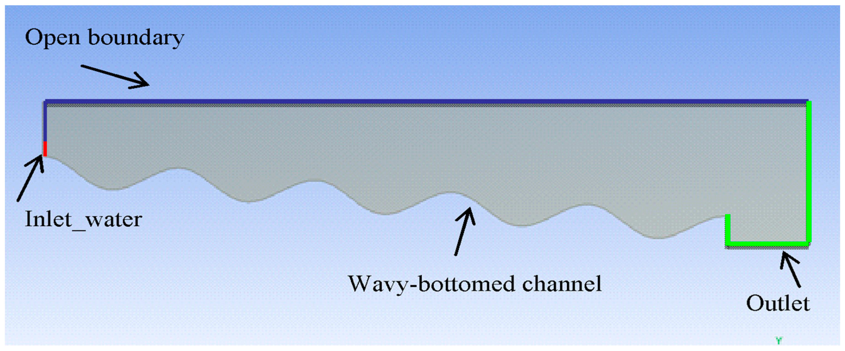
The fluid flowing through the photobioreactor was simulated for two different slopes (6° for model setup and validation and 9° for model application). Considering the channel geometry (Figure 1) and the feeding conditions, the flow is mainly two-dimensional; therefore, 2D models were used to save computational time.
The model of the wavy-bottomed channel photobioreactor at slope 6° is shown in Figure 2; the model of the channel inclined at 9° is identical to the 6° one in every aspect but the inclination slope. To limit computational burden, a 5-cavity channel was implemented instead of a 15-cavity model to mimic the experimental channel. Tests were carried out to verify that a fully developed flow was attained in each modeled cavity and that the CFD model was, therefore, equivalent to the 15-cavity channel used in the experiments (test results shown in the Supplementary Materials).
Boundary conditions are required on all the boundaries of the solution domain to define a specific fluid flow. In the present work, water was injected in the domain through an aperture 0.015 m high, specifying its mass flow. The modeled diffuser had the same shape as the experimental diffuser described later. They shared the same width, which was equal to the wavy channel width. We found that the model diffuser height did not influence simulation results. Referring to a channel 1 m wide, three flow rates per unit width were investigated: q1 = 1.11 × 10⁻³, q2 = 1.48 × 10⁻³, and q3 = 1.85 × 10⁻³ m3 s−1 m−1, respectively. No remarkable influence of the water inlet height on the results was noticed.
Atmospheric pressure was specified at the outlet, at the boundary above the inlet and at the top boundary. Lastly, the wavy-bottom channel was modeled as a no-slip wall boundary (Figure 1).
A second-order discretization scheme was chosen for the momentum, turbulent kinetic energy, and the specific dissipation rate equations; the body force-weighted pressure discretization scheme was used because of the presence of gravity, and the “geometric reconstruction” method was successful in sharpening the interface between air and water. The k-ω turbulent shear stress transport (SST) model was adopted to solve the closure scheme, owing to the prevailing flow conditions. The Reynolds number (Re = (Q/W)/ν, where Q is the flow rate, W = 0.15 m is the channel width, and ν is the kinematic viscosity of water) increases with flow rate, ranging between 1110 and 1850. The prevailing Re values suggest that the flow regime within the channel is in the transitional region, since the critical Re for an open channel is about 500. The PISO (Pressure-Implicit with Splitting of Operators) algorithm was employed because it is specifically designed for transient simulations, and a time step of 10−4 s was used to keep the simulation stable. The type, quadrangular versus triangular cells, and size of the calculation grid was chosen based on a trade-off between accuracy in describing the interface and the computational time issue. Each simulation was extended until a stable velocity field was obtained, wherefrom the recirculation time in each cavity and the time required for a neutrally buoyant particle to travel from one cavity to the subsequent one can be calculated, thus determining the light flashing experienced by cells in an operating photobioreactor of this type. The influence of the gridding scheme on the velocity profile and the progress toward the steady-state are fully documented in the Supplementary Materials.
2.2. Experimental Investigation
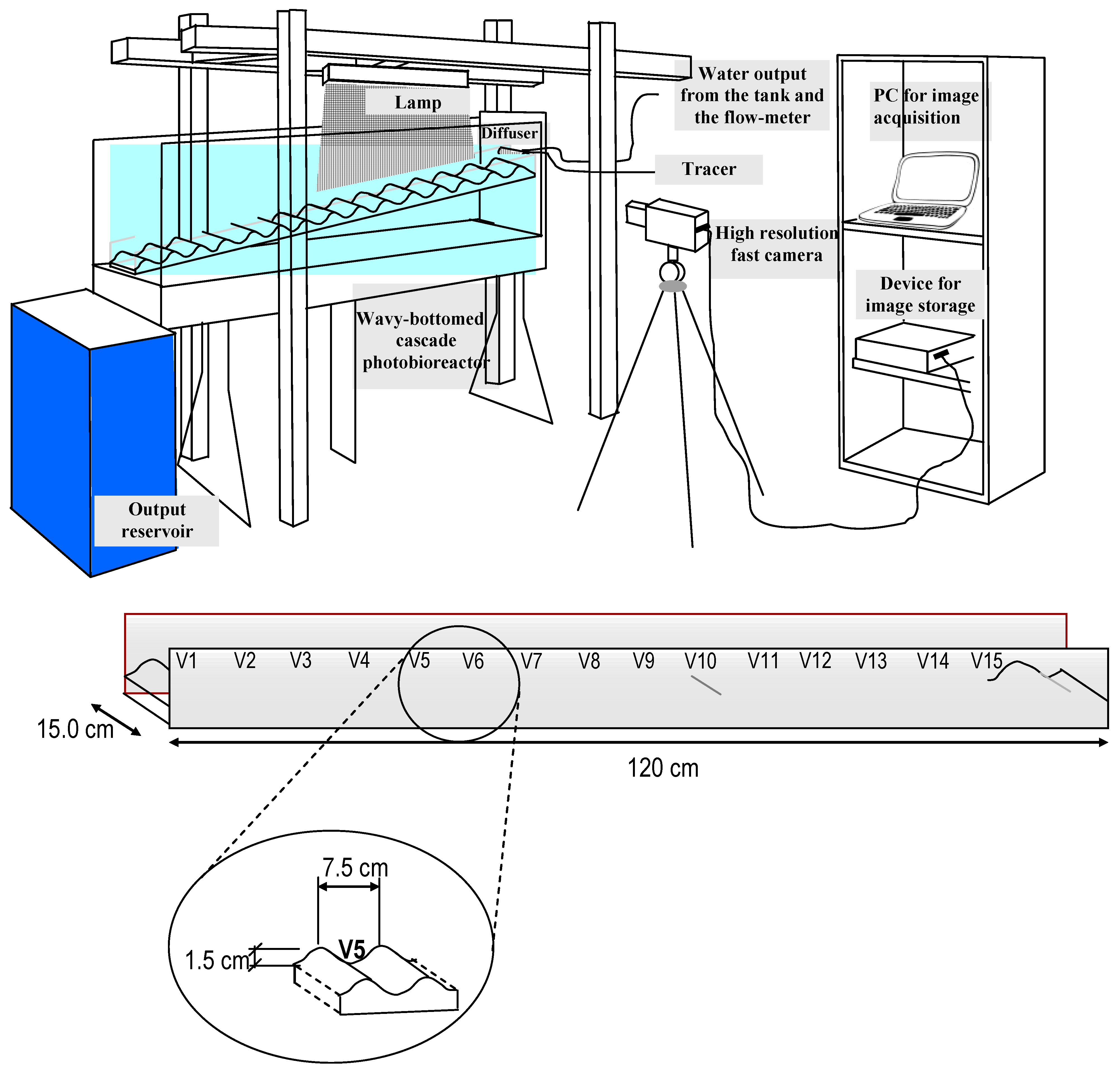
Model setup was based on experimental data collected in a test rig substantially analogous to that described by Moroni and others [19]. The wavy-bottomed channel, comprising 15 complete cavities (Figure 2), was installed at 6° slope and operated at the flow rates of Q1 = 0.6, Q2 = 0.8, and Q3 = 1.0 m3/h, corresponding to the specific flow rates numerically investigated.
Experimental investigation was carried out by feeding the channel with mixtures of water and a reflecting, neutrally buoyant passive tracer (VESTOSINT®, average diameter dp = 56 µm, density ρp = 1016 Kg/m3) via a variable height tank connected to the diffuser installed at the upper-most cavity of the channel that took a high-speed video of the flow. The illuminating device was a commercial equipment (Cobra Slim), providing a vertical sheet of light 1 cm thick along the plane of symmetry of the channel. The installed high-speed camera was capable of acquiring videos at 500 fps, but image sequences were taken at 250 fps after checking that this frequency ensured stable flow reconstruction with minimal computational burden. The acquired image sequences were elaborated by hybrid Lagrangian particle tracking (HLPT) [25] to obtain the trajectories and the velocity fields of the tracer particles. The HLPT algorithm is based on the solution of the optical flow equation and selects areas of each image where strong brilliance gradients exist. Such areas can be associated to tracer particles and are good features to track from frame to frame. Once the particles have been identified, the algorithm calculates the coordinates of the barycenter and reconstructs the trajectory of each particle, calculating their displacement in the subsequent frames.
Image processing was achieved in three steps: (1) a pre-processing step aimed to remove the background and improve image contrast, (2) particle detection and temporal tracking via HLPT to isolate particles and track them in consecutive frames, and (3) post-processing to obtain the relevant flow parameters [18].
The free surface, which from a finite distance appears as a thick zone due to the divergence of the optical axes, was excluded from analysis.
3. Results
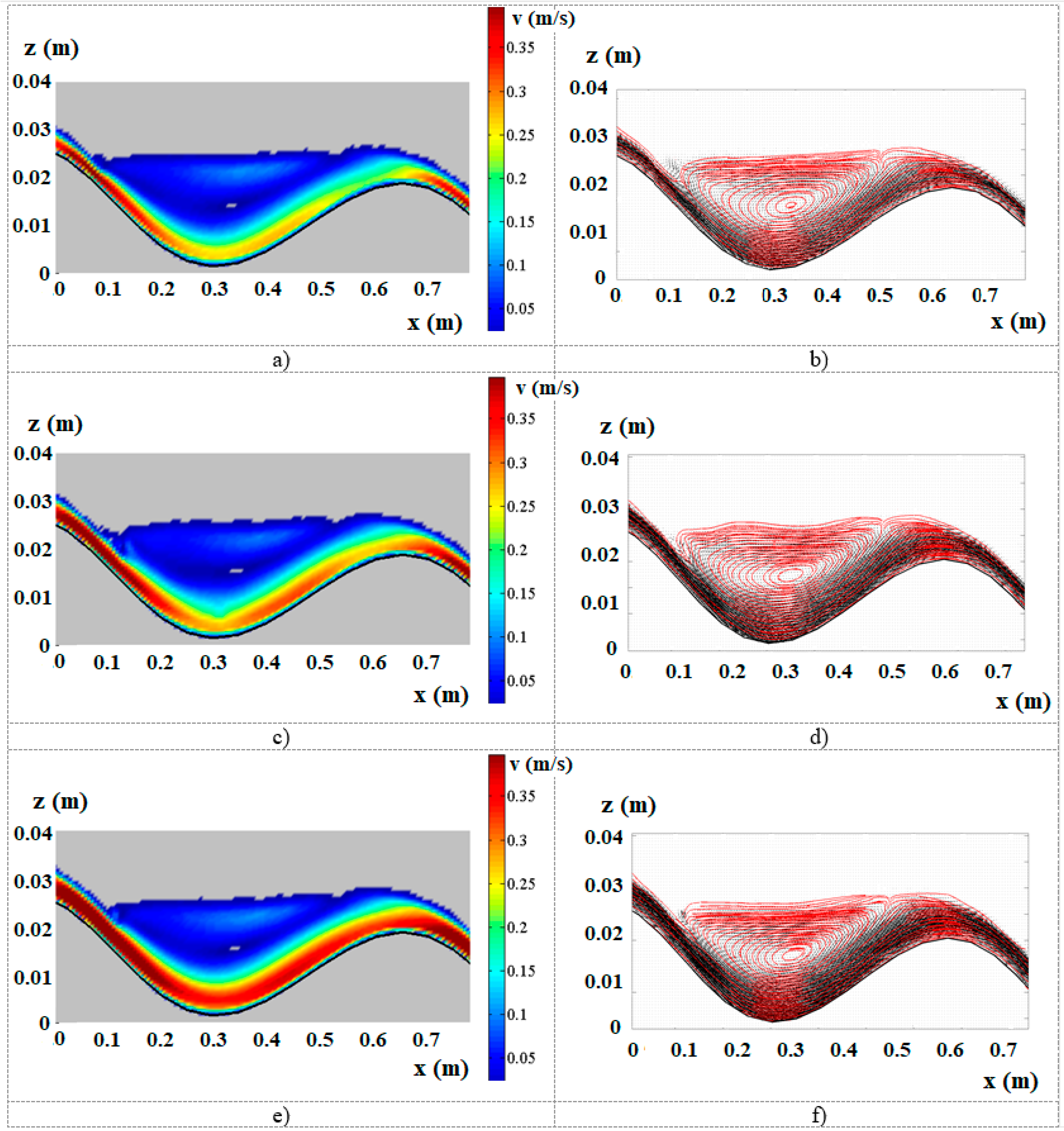
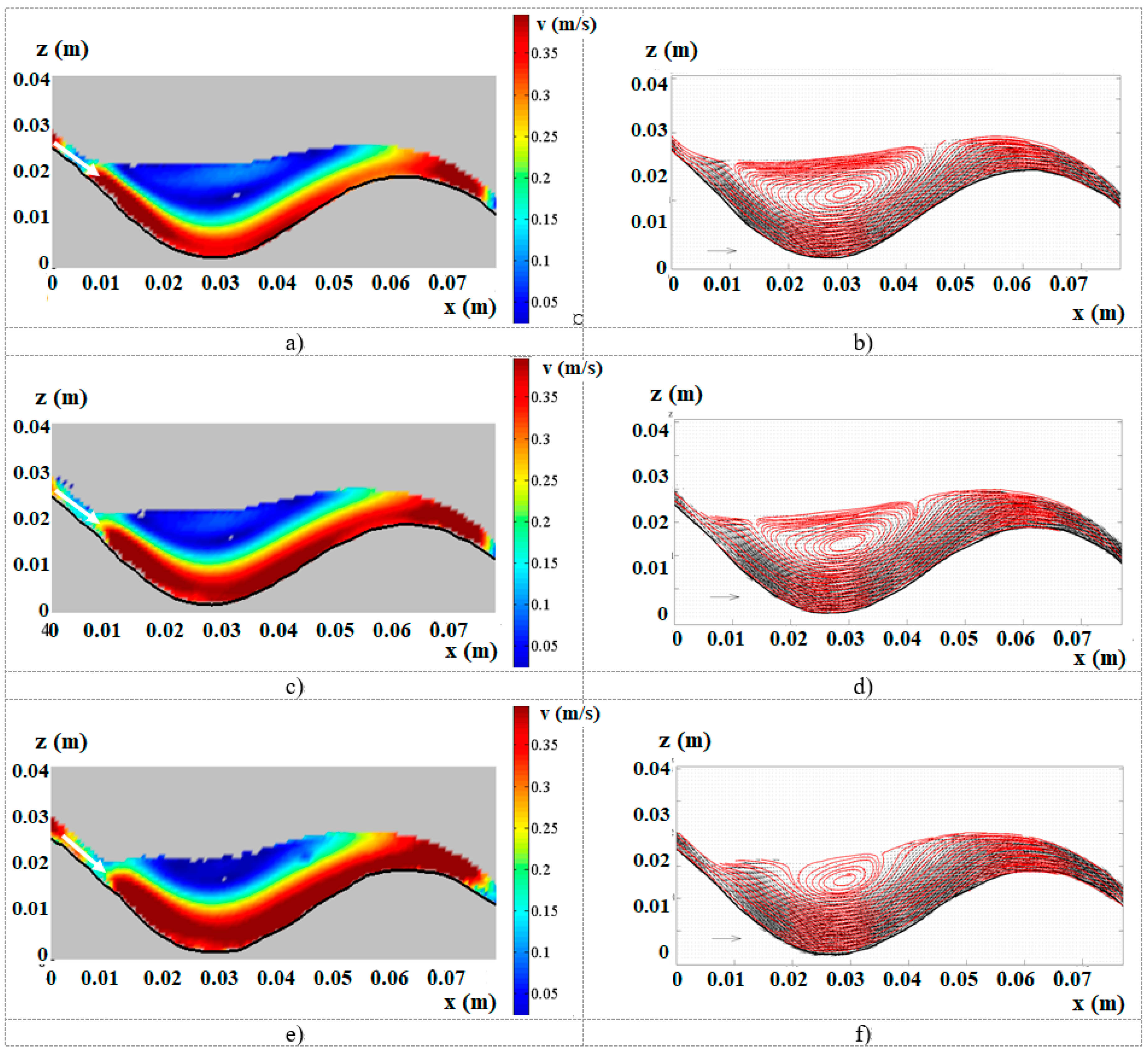
The predicted model of the velocity field and streamlines is shown in Figure 3 (the complete set of predictions can be found in the Supplementary Materials file). It showed a transport stream flowing on the bottom of the channel and a recirculation zone, which steadily occupied the central part of the cavities and represented, fairly well, the hydrodynamic features obtained from the experimental investigation (Figure 4).
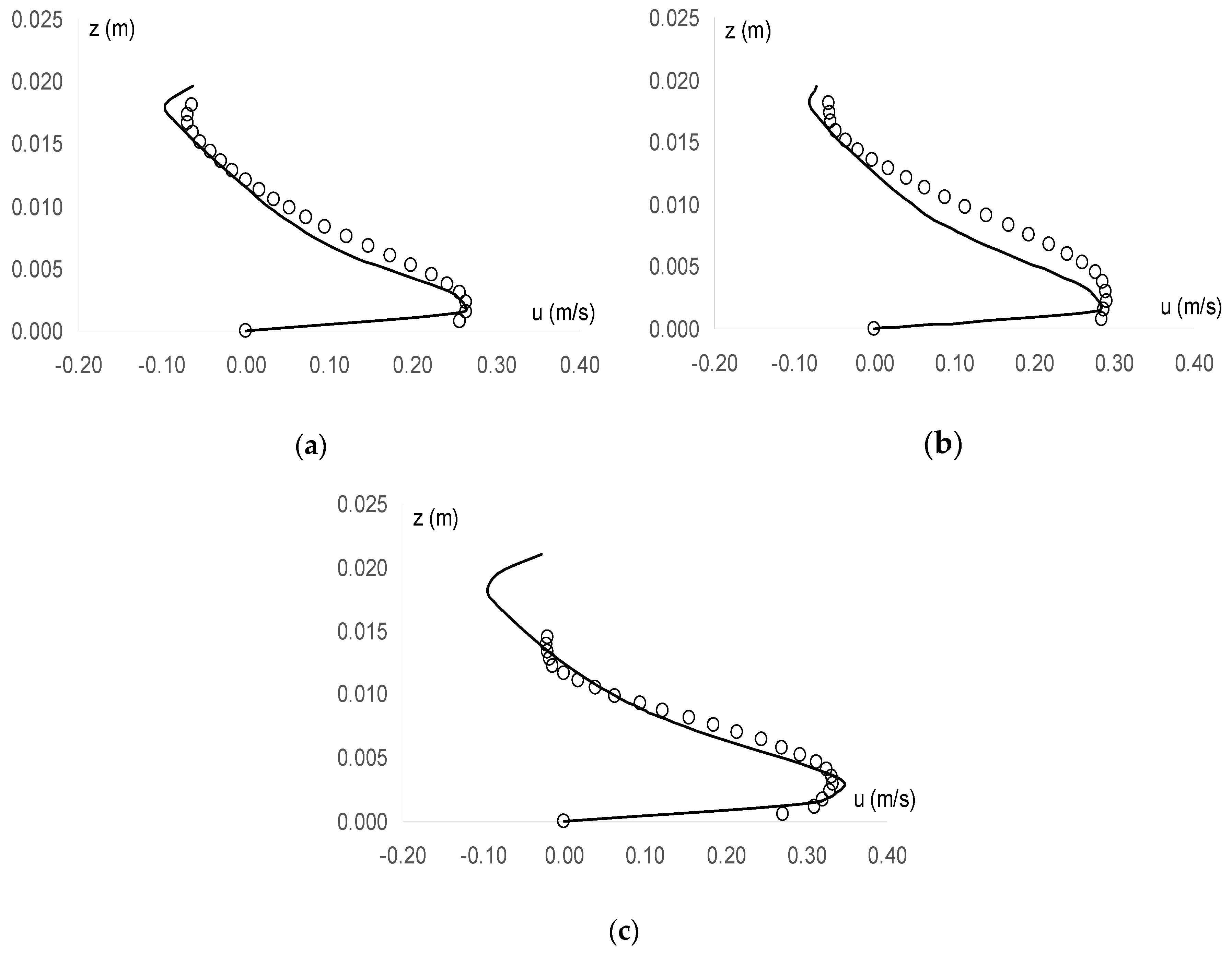
Semiquantitative validation of the numerical model was based on visually judging the agreement of the velocity profiles along the vertical section passing through the vortex center. For the three experimentally tested and computationally simulated flow rates quite a good agreement for the minimum and the intermediate flow rates was observed, with substantial agreement both in the trend and in the local values of velocity (Figure 5a,b). In the case of maximum flow rate, adherence between predicted and measured values of local velocity appeared remarkable up to the height at which experiments allowed estimating the local velocity vectors (Figure 5c).
Quantitative validation of the numerical model was performed by comparing the corresponding numeric values of the parameters describing the hydraulic features of potential photobiological significance, which are of most concern for microalgal technology. The recirculation period (tc) of the liquid elements was calculated as tc = 2π/(∂u/∂z) from the velocity plot by considering the (nearly) constant value of the velocity gradient within the vortex (∂u/∂z) and the characteristic dimensions of the vortex structure according to a previously described procedure [18].
For numerical simulations, the transport stream flow transit time was calculated by averaging the time required for individual “virtual tracers” (a feature of the Fluent environment) to travel the distance between two subsequent ridges of the wavy bottom. The size of the recirculation zone as well as the ratio of the cross-section of fluid entrained in the tumbling structure and the entire fluid cross-section occupying each cavity were calculated from streamline plots.
Comparisons between the values of the light flash-related hydrodynamic parameters predicted by CFD and those computed from post-processed experimental data are reported in Table 1.
It can be seen that the two period-related features were extremely consistent between corresponding flow rates, as deviations were within 10%. Larger deviations can be observed for the ratio of recirculating to total cross-section, in which each feature applied only for the higher specific flow rates. This deviation was motivated by the increasingly agitated free surface, which did not undergo image analysis. The discrepancy in the total cross-section of the liquid body contained by the cavity between CFD and experimental determination was constant across specific flow rates, and it was largely justified by the agitated free surface effect as well.
The CFD model was validated by attempting to predict the flow conditions that would establish if a wavy channel with the same geometry was installed with a higher slope (i.e., 9°). The simulations relevant to the channel inclined by 9° were characterized by the presence of a less-stable free surface with respect to that obtained in the 6° inclination cases. Furthermore, the recirculation areas, although they were present, fluctuated over time, never settling in a well-defined zone of the cavity.
Companion experimental tests were, therefore, performed with the channel slope set at 9° to assess the validity of CFD predictions. Post-processed experimental data did not show recirculations at larger specific flow rates (Q2 = 0.8 and Q3 = 1.0 m3/h, corresponding to 1.48 × 10⁻³ and 1.85 × 10⁻³ m3 s−1 m−1 specific flow rates), while a small recirculation area was visible at the lower specific test flow rate (Q1 = 0.6 m3/h, corresponding to 1.11 × 10⁻³ m3 s−1 m−1). A deeper analysis carried out by visualizing the experimental tracer particles trajectories showed, however, that recirculation sections still appeared at higher specific flow rates, but the positions of the centers of such recirculation sections fluctuated; thus, they did not appear in streamline plots as a consequence of the averaging of velocity fields over the whole acquisition time of the experimental run. A constant finding of this closer observation is that the observed moving-center recirculation zones were always above the transport stream. These findings appear very consistent and show that the developed CFD model is very robust and reliable.
Even in the absence of significant recirculation areas within the cavity, the transport stream produced alternations of light and darkness, and the validated model at 9° slope was, therefore, used to attempt calculating the characteristic period (transport stream flow transit time) and the cross-sections that had a photobiological significance (Table 2). As a matter of fact, the 6° to 9° increase in channel slope did not produce a significant decrease of the recirculation period.
The lowest recirculatory period of the tested installation slopes was 0.27 s (for both 6° and 9° slopes) with scarcely significant differences among test cases (the maximum period was 0.29 s). The lowest top-bottom straight transit time was 0.18 s (9° slope), corresponding to flashing frequencies of 3.7 and 5.6 Hz, respectively. The validated CFD model might be reliably used to improve results by optimizing relevant aspects of the geometry (pitch—i.e., distance between subsequent cavities of the wavy bottom—and inclination) and operation (specific flow rate) of the sloping wavy photobioreactor, hunting for an optimal synergism of the entailed flashing-light effects and mass transfer efficiency, and thereby improving microalgal productivity.
4. Conclusions
The present work shows that CFD modeling is capable of accurately predicting hydrodynamic parameters that are relevant for photobiology, such as the recirculating and transport stream flow periods (within 10%) of stable flows. The robustness of the developed model was demonstrated by successful prediction of the flow behavior at a higher installation inclination of the wavy channel, where unstable recirculations that were clearly visible in the CFD streamlines matched unstable recirculations that could be spotted by inspecting the experimental trajectories. The lowest recirculatory period of the tested installation slopes was 0.27 s, and the lowest top-bottom straight transit time was 0.18 s, corresponding to flashing frequencies of 3.7 and 5.6 Hz, respectively.
The reliability of the presented CFD model paves the way for multiple development scenarios in the research to come. Future research includes (1) improving the flashing light frequency-related aspects of the geometry (pitch and inclination) and operation (specific flow rate) of the sloping wavy photobioreactor, (2) developing a coupled fluid dynamic-cell photobiology model for the forecast of microalgal productivity of the bare photobioreactor, and (3) experimentally validating the photobioreactor, including the recirculation device with a living culture in controlled, high-irradiance experimental conditions and real-life outdoor operation.
Supplementary Materials
The following are available online at https://www.mdpi.com/2073-4441/11/7/1521/s1, Figure S1: Model domain with (a) quadrangular and (b) triangular mesh cells, Figure S2: Color maps of the water volume fraction obtained by employing the (a) implicit Volume of Fraction and (b) explicit Volume of Fraction models (recall that the red color represents water, while blue air), Figure S3: Comparison of the interface for quadrangular cells of (a) 10−3 m, (b) 2 × 10⁻³ m and (c) 3 × 10⁻³ m size, Figure S4: Time history of the water volume fraction, Figure S5: Streamlines from numerical data for 6° slope and flow rate per unit width a) 1.11 × 10⁻³ m3 s−1 m−1; b) 1.48 × 10⁻³ m3 s−1 m−1 and c) 1.85 × 10⁻³ m3 s−1 m−1 (streamlines refer to the condition reached at simulation time = 4 s with 1 mm quadrilateral calculation grid), Figure S6: Streamlines from experimental data for 6° slope and flow rate per unit width a) 1.11 × 10⁻³ m3 s−1 m−1; b) 1.48 × 10⁻³ m3 s−1 m−1 and c) 1.85 × 10⁻³ m3 s−1 m−1, Figure S7: Magnification of a single vane (slope 9°, specific flow rate = 1.48 × 10⁻³ m3 s−1 m−1).
Author Contributions
Conceptualization, M.M. and A.C.; Investigation, M.M. and S.L.; Supervision, M.B.
Funding
This research received no external funding. APC was covered by internal funding of Sapienza Università di Roma.
Conflicts of Interest
The authors declare no conflict of interest.
References
- Kim, Z.H.; Kim, S.H.; Lee, H.S.; Lee, C.G. Enhanced production of astaxanthin by flashing light using Haematococcus pluvialis. Enzym. Microb. Technol. 2006, 39, 414–419. [Google Scholar] [CrossRef]
- Pruvost, J.; Le Borgne, F.; Artu, A.; Cornet, J.F.; Legrand, J. Industrial photobioreactors and scale-up concepts. In Advances in Chemical Engineering; Academic Press: Cambridge, MA, USA, 2016; Volume 48, pp. 257–310. [Google Scholar]
- Raven, J.A. The cost of photoinhibition. Physiol. Plant. 2011, 142, 87–104. [Google Scholar] [CrossRef] [PubMed]
- Grobbelaar, J.U. Upper limits of photosynthetic productivity and problems of scaling. J. Appl. Phycol. 2009, 21, 519–522. [Google Scholar] [CrossRef]
- Vejrazka, C.; Janssen, M.; Streefland, M.; Wijffels, R.H. Photosynthetic efficiency of Chlamydomonas reinhardtii in attenuated, flashing light. Biotechnol. Bioeng. 2012, 109, 2567–2574. [Google Scholar] [CrossRef] [PubMed]
- Xue, S.; Zhang, Q.; Wu, X.; Yan, C.; Cong, W. A novel photobioreactor structure using optical fibers as inner light source to fulfill flashing light effects of microalgae. Bioresour. Technol. 2013, 138, 141–147. [Google Scholar] [CrossRef] [PubMed]
- Graham, P.J.; Nguyen, B.; Burdyny, T.; Sinton, D. A penalty on photosynthetic growth in fluctuating light. Sci. Rep. 2017, 7, 1–11. [Google Scholar] [CrossRef] [PubMed] [Green Version]
- Grobbelaar, J.U. Photosynthetic response and acclimation of microalgae to light fluctuations. In Algal Cultures, Analogues of Blooms and Applications; Subba Rao, D.V., Ed.; Science Publishers: Enfield, CT, USA, 2006; pp. 671–683. [Google Scholar]
- Richmond, A. Efficient utilization of high irradiance for production of photoautotropic cell mass: A survey. J. Appl. Phycol. 1996, 8, 381–387. [Google Scholar] [CrossRef]
- Abu-Ghosh, S.; Fixler, D.; Dubinsky, Z.; Iluz, D. Flashing light in microalgae biotechnology. Bioresour. Technol. 2016, 203, 357–363. [Google Scholar] [CrossRef]
- Gordon, J.M.; Polle, J.E. Ultrahigh bioproductivity from algae. Appl. Microbiol. Biotechnol. 2007, 76, 969–975. [Google Scholar] [CrossRef]
- Qiang, H.; Richmond, A. Productivity and photosynthetic efficiency of Spirulina platensis as affected by light intensity, algal density and rate of mixing in a flat plate photobioreactor. J. Appl. Phycol. 1996, 8, 139–145. [Google Scholar] [CrossRef]
- Grobbelaar, J.U. Turbulence in mass algal cultures and the role of light/dark fluctuations. J. Appl. Phycol. 1994, 6, 331–335. [Google Scholar] [CrossRef]
- Scarsella, M.; Torzillo, G.; Cicci, A.; Belotti, G.; De Filippis, P.; Bravi, M. Mechanical stress tolerance of two microalgae. Process. Biochem. 2011, 47, 1603–1611. [Google Scholar] [CrossRef]
- Cicci, A.; Stoller, M.; Moroni, M.; Bravi, M. Mass Transfer, Light Pulsing and Hydrodynamic Stress Effects in Photobioreactor Development. Chem. Eng. Trans. 2015, 43, 235–240. [Google Scholar]
- Torzillo, G.; Giannelli, L.; Verdone, N.; De Filippis, P.; Scarsella, M.; Martínez-Roldán, A.J.; Bravi, M. Microalgae Culturing in Thin-layer Photobioreactors. Chem. Eng. Trans. 2010, 20, 265–270. [Google Scholar]
- Setlik, I.; Veladimir, S.; Malek, I. Dual purpose open circulation units for large scale culture of algae in temperature zones. I. Basic design considerations scheme of pilot plant. Algol Stud. (Trebon) 1970, 1, 111–164. [Google Scholar]
- Moroni, M.; Cicci, A.; Bravi, M. Experimental investigation of a local recirculation photobioreactor for mass cultures of photosynthetic microorganisms. Water Res. 2014, 52, 29–39. [Google Scholar] [CrossRef]
- Sforza, E.; Simionato, D.; Giacometti, G.M.; Bertucco, A.; Morosinotto, T. Adjusted light and dark cycles can optimize photosynthetic efficiency in algae growing in photobioreactors. PLoS ONE 2012, 7, e38975. [Google Scholar] [CrossRef]
- Soman, A.; Shastri, Y. Optimization of novel photobioreactor design using computational fluid dynamics. Appl. Energy 2015, 140, 246–255. [Google Scholar] [CrossRef]
- Gómez-Pérez, C.A.; Espinosa, J.; Ruiz, L.M.; Van Boxtel, A.J.B. CFD simulation for reduced energy costs in tubular photobioreactors using wall turbulence promoters. Algal Res. 2015, 12, 1–9. [Google Scholar] [CrossRef]
- Cho, B.A.; Pott, R.W.M. The development of a thermosiphon photobioreactor and analysis using Computational Fluid Dynamics (CFD). Chem. Eng. J. 2019, 363, 141–154. [Google Scholar] [CrossRef]
- Adesanya, V.O.; Vadillo, C.D.; Mackley, M.R. The rheological characterization of algae suspensions for the production of biofuels. J. Rheol. 2012, 56, 925–939. [Google Scholar] [CrossRef] [Green Version]
- Hirt, C.W.; Nichols, B.D. Volume of Fluid (VOF) Method for Dynamics of Free Boundaries. J. Comput. Phys. 1981, 39, 201. [Google Scholar] [CrossRef]
- Moroni, M.; Lupo, E.; La Marca, F. Investigation on an innovative technology for wet separation of plastic wastes. Waste Manag. 2017, 66, 13–22. [Google Scholar] [CrossRef] [PubMed]
Figure 1.
Experimental setup and the channel featuring characteristic dimensions. V stands for vane.
Figure 1.
Experimental setup and the channel featuring characteristic dimensions. V stands for vane.

Figure 2.
Model geometry and boundary conditions of the photobioreactor at slope 6°.

Figure 3.
Computational fluid dynamic (CFD) colormap results for 6° slope and flow rate per unit width (a) q1, (b) q2, and (c) q3. Streamlines at flow rate per unit width (d) q1, (e) q2, and (f) q3.
Figure 3.
Computational fluid dynamic (CFD) colormap results for 6° slope and flow rate per unit width (a) q1, (b) q2, and (c) q3. Streamlines at flow rate per unit width (d) q1, (e) q2, and (f) q3.

Figure 4.
Experimental colormap results for 6° slope and flow rate per unit width (a) q1, (b) q2, and (c) q3. Streamlines at flow rate per unit width (d) q1, (e) q2, and (f) q3.
Figure 4.
Experimental colormap results for 6° slope and flow rate per unit width (a) q1, (b) q2, and (c) q3. Streamlines at flow rate per unit width (d) q1, (e) q2, and (f) q3.

Figure 5.
Experimental (open dots) and numerical (continuous line) profiles of local liquid velocities along the vertical lines passing through the center of the recirculation areas that were established inside each cavity for the flow rates per unit width (a) 1.11 × 10⁻³, (b) 1.48 × 10⁻³, and (c) 1.85 × 10⁻³ m3 s−1 m−1.


Table 1.
Comparisons of experimentally determined and numerically simulated hydraulic features of potential photobiologic significance for the 6° channel slope.
Table 1.
Comparisons of experimentally determined and numerically simulated hydraulic features of potential photobiologic significance for the 6° channel slope.
| Flow Rate per Unit Width (m3 s−1 m−1) | Recirculation Period (s) | Transport Stream Flow Transit Time (s) | Recirculation Area (10−4 m2) | Total Cross- Section (10−4 m2) | Ratio of Recirculating Area to Total Cross-Section | |||||
|---|---|---|---|---|---|---|---|---|---|---|
| Exp | Num | Exp | Num | Exp | Num | Exp | Num | Exp | Num | |
| 1.11 × 10⁻³ | 0.37 | 0.34 | 0.31 | 0.31 | 3.83 | 4.43 | 8.58 | 9.27 | 0.45 | 0.48 |
| 1.48 × 10⁻³ | 0.34 | 0.33 | 0.27 | 0.26 | 2.91 | 4.32 | 9.12 | 9.45 | 0.32 | 0.43 |
| 1.85 × 10⁻³ | 0.27 | 0.29 | 0.25 | 0.23 | 2.14 | 3.97 | 9.23 | 9.87 | 0.23 | 0.40 |
Table 2.
Hydraulic features of potential photobiologic significance for validated model at 9° slope.
Table 2.
Hydraulic features of potential photobiologic significance for validated model at 9° slope.
| Flow Rate per Unit Width. (m3 s−1 m−1) | Recirculation Period (s) | Transport Stream Flow Transit Time (s) | Recirculation Area (10−4 m2) | Total Cross-Section (10−4 m2) | Ratio of Recirculating to Total Cross-Section |
|---|---|---|---|---|---|
| 1.11 × 10⁻³ | 0.28 | 0.25 | 3.36 | 6.79 | 0.49 |
| 1.48 × 10⁻³ | 0.29 | 0.23 | 3.31 | 7.84 | 0.42 |
| 1.85 × 10⁻³ | 0.27 | 0.18 | 2.39 | 8.18 | 0.33 |
© 2019 by the authors. Licensee MDPI, Basel, Switzerland. This article is an open access article distributed under the terms and conditions of the Creative Commons Attribution (CC BY) license (http://creativecommons.org/licenses/by/4.0/).
Share and Cite
MDPI and ACS Style
Moroni, M.; Lorino, S.; Cicci, A.; Bravi, M. Design and Bench-Scale Hydrodynamic Testing of Thin-Layer Wavy Photobioreactors. Water 2019, 11, 1521. https://doi.org/10.3390/w11071521
AMA Style
Moroni M, Lorino S, Cicci A, Bravi M. Design and Bench-Scale Hydrodynamic Testing of Thin-Layer Wavy Photobioreactors. Water. 2019; 11(7):1521. https://doi.org/10.3390/w11071521
Chicago/Turabian StyleMoroni, Monica, Simona Lorino, Agnese Cicci, and Marco Bravi. 2019. "Design and Bench-Scale Hydrodynamic Testing of Thin-Layer Wavy Photobioreactors" Water 11, no. 7: 1521. https://doi.org/10.3390/w11071521
Note that from the first issue of 2016, this journal uses article numbers instead of page numbers. See further details here.