Parameters Estimation and Prediction of Water Movement and Solute Transport in Layered, Variably Saturated Soils Using the Ensemble Kalman Filter

Abstract

The parameters of water movement and solute transport models are essential for the accurate simulation of soil moisture and salinity, particularly for layered soils in field conditions. Parameter estimation can be achieved using the inverse modeling method. However, this type of method cannot fully consider the uncertainties of measurements, boundary conditions, and parameters, resulting in inaccurate estimations of parameters and predictions of state variables. The ensemble Kalman filter (EnKF) is well-suited to data assimilation and parameter prediction in Situations with large numbers of variables and uncertainties. Thus, in this study, the EnKF was used to estimate the parameters of water movement and solute transport in layered, variably saturated soils. Our results indicate that when used in conjunction with the HYDRUS-1D software (University of California Riverside, California, CA, USA) the EnKF effectively estimates parameters and predicts state variables for layered, variably saturated soils. The assimilation of factors such as the initial perturbation and ensemble size significantly affected in the simulated results. A proposed ensemble size range of 50–100 was used when applying the EnKF to the highly nonlinear hydrological models of the present study. Although the simulation results for moisture did not exhibit substantial improvement with the assimilation, the simulation of the salinity was significantly improved through the assimilation of the salinity and relative solutetransport parameters. Reducing the uncertainties in measured data can improve the goodness-of-fit in the application of the EnKF method. Sparse field condition observation data also benefited from the accurate measurement of state variables in the case of EnKF assimilation. However, the application of the EnKF algorithm for layered, variably saturated soils with hydrological models requires further study, because it is a challenging and highly nonlinear problem.

1. Introduction

The soil moisture status of farmland is crucial for optimizing irrigation water management, which promotes efficient water use and alleviates soil secondary salinity problems. In field conditions, soils exhibit a vertically layered distribution and are variably saturated due to infiltration and evaporation. Soil water and salinity are commonly estimated or predicted using the Richards equation and convection–dispersion equation-based models, respectively.

The estimation and prediction of soil moisture and salinity are imprecise because of inherent process uncertainties, such as the model parameters [1], initial and boundary conditions [2], and source/sink relationships in the root zone, particularly for layered, variably saturated soils. Thus, there is a great need for methods that can improve the accuracy of simulation results or parameter estimation via inverse modeling [3]. The accuracy of modeling and prediction can be improved by optimizing the parameters through a calibration process [4] or by directly updating the state variables involved in the modeling process [5]. Both types of improvements require exploiting observations associated with the model state variables. However, observations can introduce errors due to instrument inaccuracy.

Optimal parameter values can be obtained using inverse modeling. Various inverse modeling methods have been developed, including the annealing–simplex method [6], genetic algorithms [7], multilevel grid sampling strategies [8], ant colony optimization [9], shuffled complex methods [10], the Shuffled Complex Evolution Metropolis algorithm [11], and the multi-algorithm genetically adaptive method [12]. Although these methods account for the uncertainties of model parameters, they do not explicitly consider the uncertainties of inputs and outputs, as well as those of the model [13]. Therefore, such treatments may produce suboptimal parameter values and correspondingly inaccurate models and forecasts.

The recently developed ensemble Kalman filter (EnKF) [14] has been widely used in hydrological processes for data assimilation and parameterization [15,16,17] because of its comprehensive consideration of uncertainties. Moreover, the EnKF is well-suited to multi-dimensional systems and nonlinear problems [14] owing to its titular ensemble forecasting technique. The EnKF method is particularly noted for its robustness when applied to state assimilation and parameters estimation for hydrological modeling. For example, Xie and Zhang [18] obtained acceptable parameters and satisfactory estimations of the runoff, soil water content, and evapotranspiration in the Soil & Water Assessment Tool model using the EnKF method. Li et al. [19] enhanced the accuracy of the estimation of the conductivities and piezometric heads in a transient groundwater flow by coupling ensemble Kalman filtering with an upscaling method. Wanders et al. [20] applied a dual state and parameter EnKF to calibrate the hydrological LISFLOOD model and used the discharge and remotely sensed soil moisture to improve the estimation of groundwater and routing parameters. Zhang et al. [21] examined the benefits of assimilating groundwater levels using different EnKF-based methodologies to improve the predictions of root zone soil moisture with an integrated terrestrial system model.

The EnKF has also been used in data assimilation for soil water movement and solute transport systems [22,23,24,25,26]. For example, Li and Ren [27] investigated the influence of assimilation factors, including the initial parameter estimate, ensemble size, observation error, model error, assimilation interval, and water regime, on soil hydraulic parameter estimation for 12 synthetic unsaturated soils. Song et al. [28] compared the performance of different iterative EnKFs (i.e., the confirming EnKF, restart EnKF, and modified restart EnKF) for the estimation of unsaturated soil hydraulic parameters. Gharamti et al. [29] used an efficient sequential data assimilation scheme based on a hybrid formulation of EnKF and optimal interpolation to accurately estimate the aquifer contamination and spatially variable sorption coefficients in a saturated heterogeneous clayey sandstone zone. However, to our knowledge, there is limited research on the application of the EnKF method for water movement and solute transport in field conditions, particularly for data from soil sampling in layered soil textures.

The objectives of the present study were as follows:

(i)

Extend the EnKF framework to estimate the parameters of water movement and solute transport in layered, variably saturated soils with field sampling data.

(ii)

Improve the prediction accuracy of soil moisture and salinity status under field conditions.

2. Materials and Methods

2.1. Governing Equations for Water Flow and Solute Transport in Variably Saturated Soils

Water flow in soils are most commonly described using the one-dimensional Richards equation [30]:

$$\frac{\partial \theta }{\partial t}=\frac{\partial }{\partial z}\left[K\left(\frac{\partial h}{\partial z}+\cos \alpha \right)\right]-S\left(h\right)$$

(1)

where θ represents the volumetric water content (cm³ cm⁻³), h represents the water pressure head (cm), t represents time (d), z represents the vertical space coordinate (cm), α represents the angle between the direction of water flow and the vertical direction, K represents the hydraulic conductivity function (cm day⁻¹), and S is the sink term (cm³ cm⁻³ day⁻¹), which is defined as the rate of root water uptake.

The soil hydraulic properties can be expressed using the equations of van Genuchten [31] and Mualem [32], which take the following forms:

$$\theta \left(h\right)=\{\begin{array}{ll}{\theta }_r+\frac{{\theta }_s-{\theta }_r}{{\left[1+{\left(\alpha \left|h\right|\right)}^n\right]}^m}& h<0\\ {\theta }_s& h\ge 0\end{array}$$

(2)

$$K\left(h\right)=K_s{S}_e^l{\left[1-{\left(1-S_e^{1/m}\right)}^m\right]}^2$$

(3)

$$S_e=\frac{\theta -{\theta }_r}{{\theta }_s-{\theta }_r}$$

(4)

where S_e represents the effective saturation (-), θ_r and θ_s represent the residual and saturated water contents (cm³ cm⁻³), respectively, K_s represents the saturated hydraulic conductivity (cm day⁻¹), α (cm⁻¹), m (-), and n (-) are empirical shape parameters, m = 1 − 1/n, and l (-) is the pore connectivity parameter with the common assumption that l = 0.5.

The solute transport can be described using the convection–dispersion equation:

$$\frac{\partial \left(\theta c\right)}{\partial t}+\frac{\partial \left(\rho s\right)}{\partial t}=\frac{\partial }{\partial z}\left(\theta D\frac{\partial c}{\partial z}\right)-\frac{\partial \left(qc\right)}{\partial z}$$

(5)

where c represents the solute concentration in the liquid phase (mg cm⁻³ or g L⁻¹), ρ represents the bulk density (g cm⁻³), s represents the adsorbed concentration (g g⁻¹), q represents the vertical water flux (cm day⁻¹), and D represents the diffusion–dispersion coefficient (cm² day⁻¹).

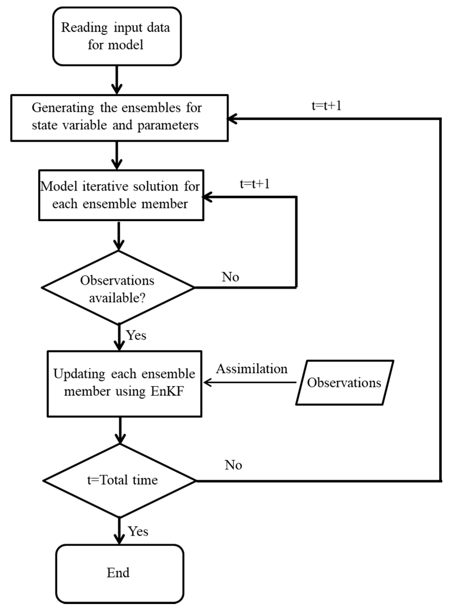
2.2. Framework of EnKF

The EnKF was first proposed by Evensen [14]. It is based on forecasting error statistics using the Monte Carlo method. This method adopts the mean of the ensemble of model states evolved in the state space as the best estimate and the spreading of the ensemble as the error variance [32]. The EnKF operates sequentially by performing a forecast step, followed by a filter update step. Generally, the forecast step for an ensemble member i between times k + 1 and k can be expressed as:

$$X_{i,k+1}^f=F_k(X_{i,k}^a)+w_{i,k};w_{i,k}~N(0,Q_k)$$

(6)

where $X_{i,k+1}^f$ and $X_{i,k}^a$ represent the forecast state vector at time k + 1 and the updated state vector at time k, respectively, F_k(•) represents the nonlinear model operator, Q_k represents the model error covariance matrix, and w_i,k represents the perturbation of the model error.

Based on a linear correction, the filter update step at time k + 1 can be expressed as:

$$X_{i,k+1}^a=X_{i,k+1}^f+K_{k+1}\left(Y_{i,k+1}-H\left(X_{i,k+1}^f\right)\right)$$

(7)

where Y_i,k+1 is the ith observation sample obtained by adding a Gaussian noise to the actual observation and H(•) is the observation operator that maps the model states to the observation space. For detailed computation of the Kalman gain matrix at time k + 1, K_k+1, please refer to Evensen [33].

2.3. Observations in Layered, Variably Saturated Soils under Field Conditions

Using datasets including the soil texture, soil moisture, and salinity of layered, variably saturated soils were collected from a maize field in the Hetao Irrigation District, which is located in the upper reaches of the Yellow River Basin. Other information, including weather, irrigation, and crop growth data, were also collected during the growing season of the year 2013 (seeded May 2 and harvested September 21) [34].

The field was irrigated three times at rates of 112 mm in the jointing stage, 94 mm in flowering stage, and 108 mm in the filling stage. The precipitation and evaporation during the growing season were 104 and 920 mm, respectively. The soils were in a variably saturated state during the wet (irrigation and/or precipitation) and drying (evaporation) cycles. The soil profiles at a depth of 0–300 cm were divided into four layers according to the soil textures, as shown in

Table 1. Values of the van Genuchten–Mualem model parameters and dispersion length for different soil layers.

Depth (cm)	θr (cm3 cm−3)	θs (cm3 cm−3)	α (cm−1)	n (-)	Ks (cm d−1)	l (-)	L (cm)	Soil Texture
0–50	0.05	0.42	0.010	1.70	9	0.5	15	Silt loam
50–150	0.04	0.47	0.012	1.50	15	0.5	15	Silt loam
150–240	0.07	0.50	0.007	1.20	4	0.5	15	Silt loam
240–300	0.03	0.45	0.012	1.70	25	0.5	15	Silt loam

. The soil water content and salinity at depths of 0–10, 10–20, 20–40, 40–60, 60–80, and 80–100 cm were measured using soil samples collected once every 10 d from May 2 to September 21, according to the crop growing season.

2.4. Model Setup

In the simulation, we used the calibrated results of Ren et al. [34] as the initial values of the soil hydraulic parameters θ_r, θ_s, α, n, and K_s, and solute longitudinal dispersivity L, as shown in Table 1. The parameters of the root water uptake used in the simulation are presented in

Table 2. Values of parameters in water and salt stress response functions.

Parameter	Description	Values (cm)
h1	No water extraction at higher pressure heads	−0.1
h2	h below which optimal water starts	−15
h3h	h below which water uptake reduction starts at high atmospheric demand	−325
h3l	h below which water uptake reduction starts at low atmospheric demand	−450
h4	h below which water uptake is zero	−8000
h*φ	Threshold value of hφ	−2000
h*φ50	hφ at which water uptake is reduced by 50%	−6000

.

A meteorological forcing with a surface layer was specified as the upper boundary condition for water flow, while a transient specified head defined by the observed groundwater depth was used as the bottom boundary condition. For solute transport, the upper and lower boundary conditions were defined by a given concentration flux, which was based on the observed total dissolved solid of irrigation water and groundwater, respectively. The initial conditions of the soil water content and solute concentration were set according to field observations [34].

2.5. Data Assimilation Procedure

The HYDRUS-1D model was employed as an ensemble mode in the data assimilation scheme, in which the soil moisture, solute contents, and model parameters were treated as random variables. The data assimilation system predicted the states of soil water movement and solute transport, and updated the model parameters sequentially in consideration of the observations. The detailed procedures are described as follows:

(1) Construct the joint matrices for water dynamics and solute transport.

$$A=\left[\begin{array}{l}h\\ K_s\\ \alpha \end{array}\right]B=\left[\begin{array}{l}c\\ L\end{array}\right]$$

(8)

In matrix A, K_s and α represent the ensembles of the soil hydraulic parameters, and h represents the pressure heads. In matrix B, L represents the ensemble of longitudinal dispersivity, and c represents the simulated solute concentration simulated.

(2) Calculate the Kalman gain matrix K_k+1 when the observations are available at time k + 1. The Kalman gain matrix can be expressed as follows:

$$K_{k+1}=P_{k+1}^f{H}^{\mathrm{T}}{(H{P}_{k+1}^f{H}^{\mathrm{T}}+R_{k+1})}^{-1}$$

(9)

where P_k+1 represents the error covariance matrix for the predicted state at time k + 1 and R_k+1 represents the error covariance matrix for observation at time k + 1.

(3) Update matrices A and B using Equation (7).

(4) Repeat steps (1)–(3) until the end of the simulation.

A flowchart of the coupling of the EnKF with HYDRUS-1D for assimilating the soil water movement and solute transport is presented in Figure 1.

2.6. Performance Metrics

The results of data assimilation were evaluated using the following indicators: the determination coefficient (R²), mean relative error (MRE), root mean square error (RMSE), andNash and Sutcliffe model efficiency (NSE) [35,36,37].

3. Results

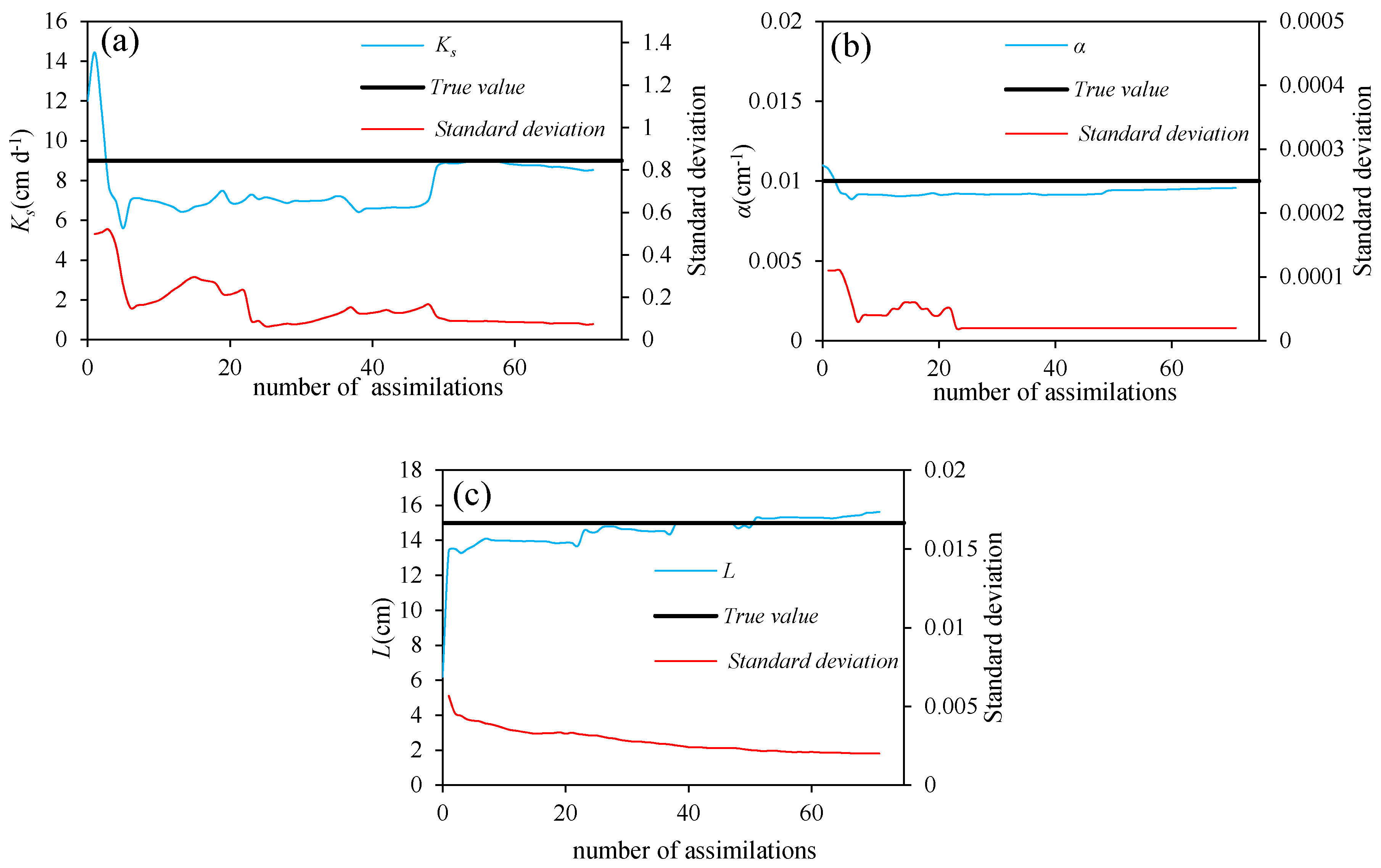
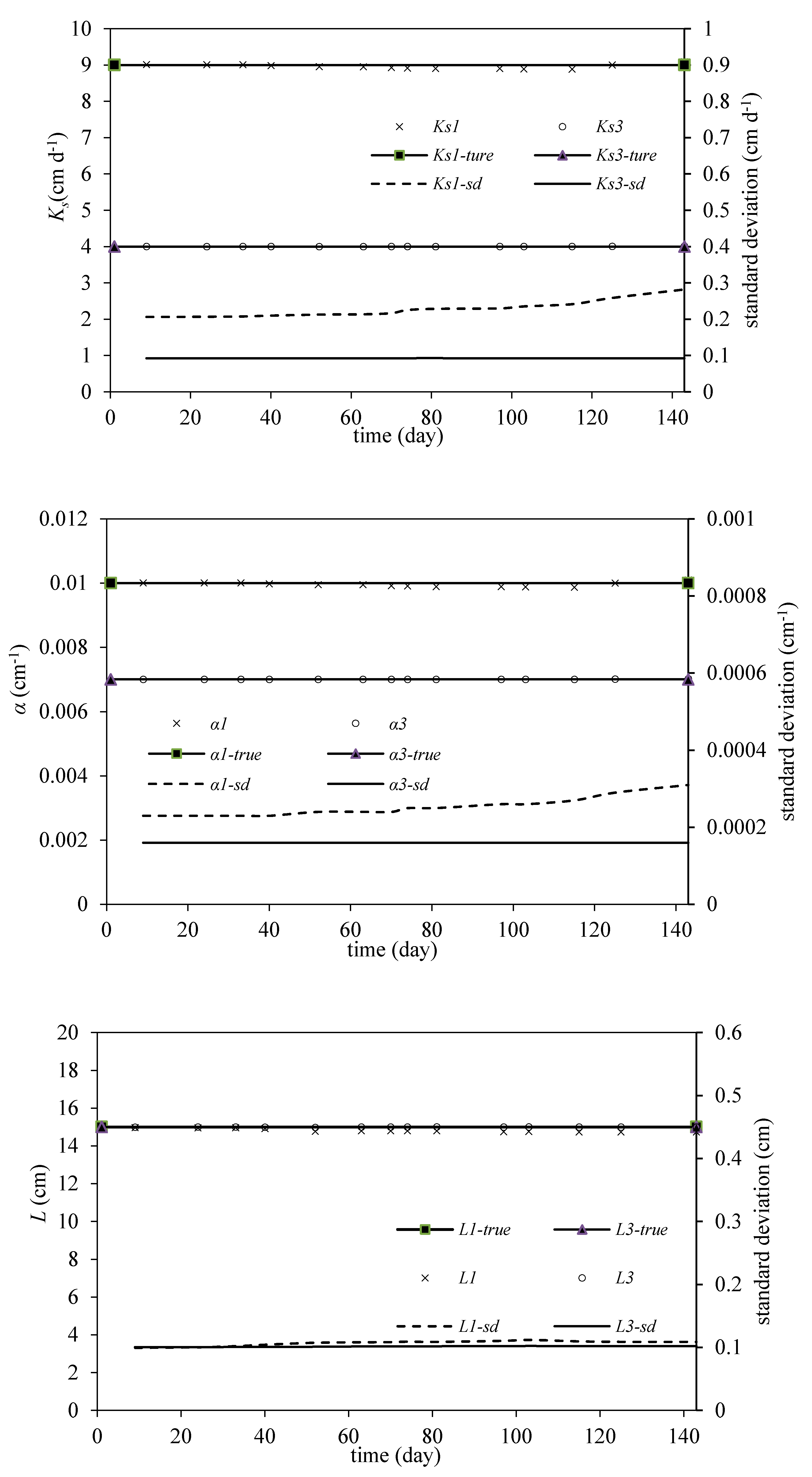
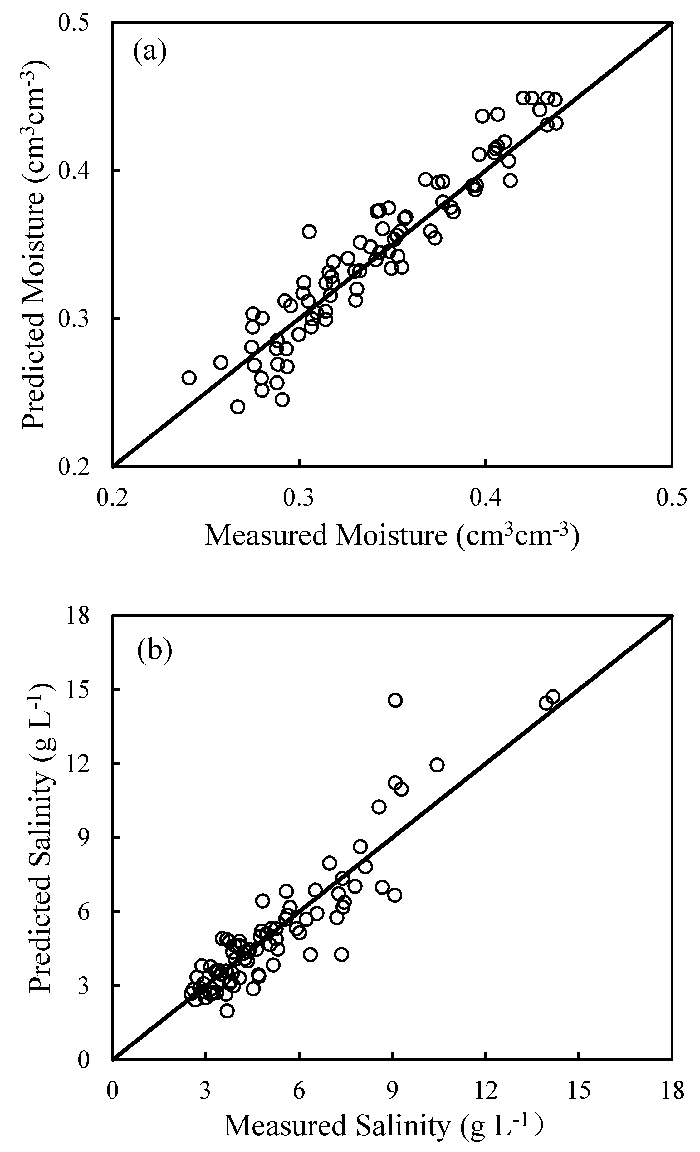
3.1. Parameter Estimation for Homogeneous Soil

First, the established assimilation scheme was applied in a synthetic experiment to verify its accuracy. The meteorological data from the study area were used as the upper boundary condition in the scheme. In situ information for the soil texture and silt loam was applied in HYDRUS-1D. The corresponding reference values of the parameters for the soil water and solute transport in assimilation were K_s = 9 cm/day, α = 0.01 cm⁻¹, and L = 15 cm. The simulated results at specific depths corresponding to the sampling scheme (5, 10, 15, 20, 30, 35, 40, 45, 50, 60, 70, 80, 90, 100, and 110 cm from the surface) were extracted for model comparison and verification. The time interval for model assimilation was set as 2 days. To evaluate the performance of the EnKF for parameter estimation, the initial estimates of K_s and α were shifted up and L was shifted down from their true values in the forecasted prior system state. Detailed information regarding the data assimilation is presented in

Table 3. Values of potential impact factors for synthetic simulation.

Factors	Values
Initial estimate of Ks (cm/day)	12
Initial estimate of α (cm−1)	0.011
Initial estimate of L (cm)	6.2
Initial standard deviation of lnKs	0.1
Initial standard deviation of lnα	0.01
Initial standard deviation of L	0.1
Model standard deviation of water content	0.001
Model standard deviation of salinity	0.01
Observation standard deviation of water content	0.0004
Observation standard deviation of salinity	0.0004
Initial standard deviation of water content	0.001
Initial standard deviation of salinity	0.01

.

The results of parameter estimation are depicted in Figure 2. We found that all the parameters for water movement and solute transport eventually approached the reference values. Among the three parameters, L exhibited a fast convergence. The changes of α and L were relatively stable, but K_s changed drastically during the process. This tendency is attributed to the larger difference between the initial estimate and the true value for K_s compared with those for α and L. The standard deviations of all the parameters decreased continuously during assimilation. Thus, in summary, the EnKF is effective for estimating the parameters of water and solute transport in homogeneous soil.

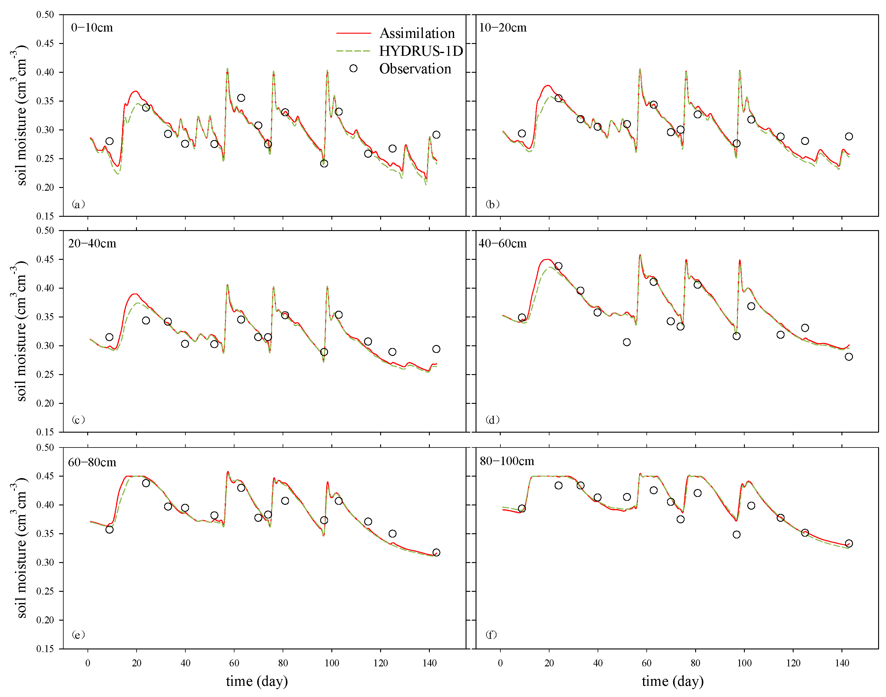
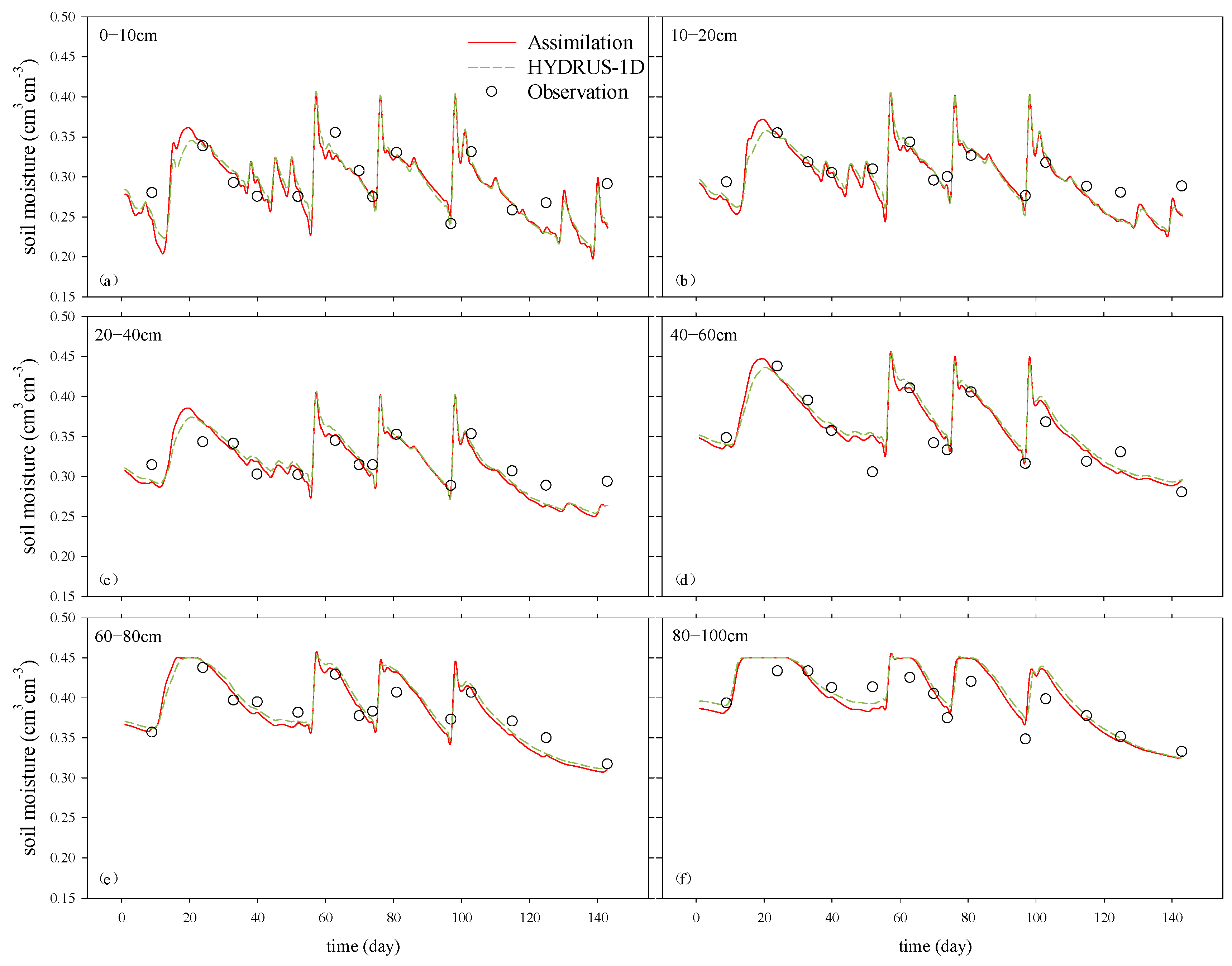
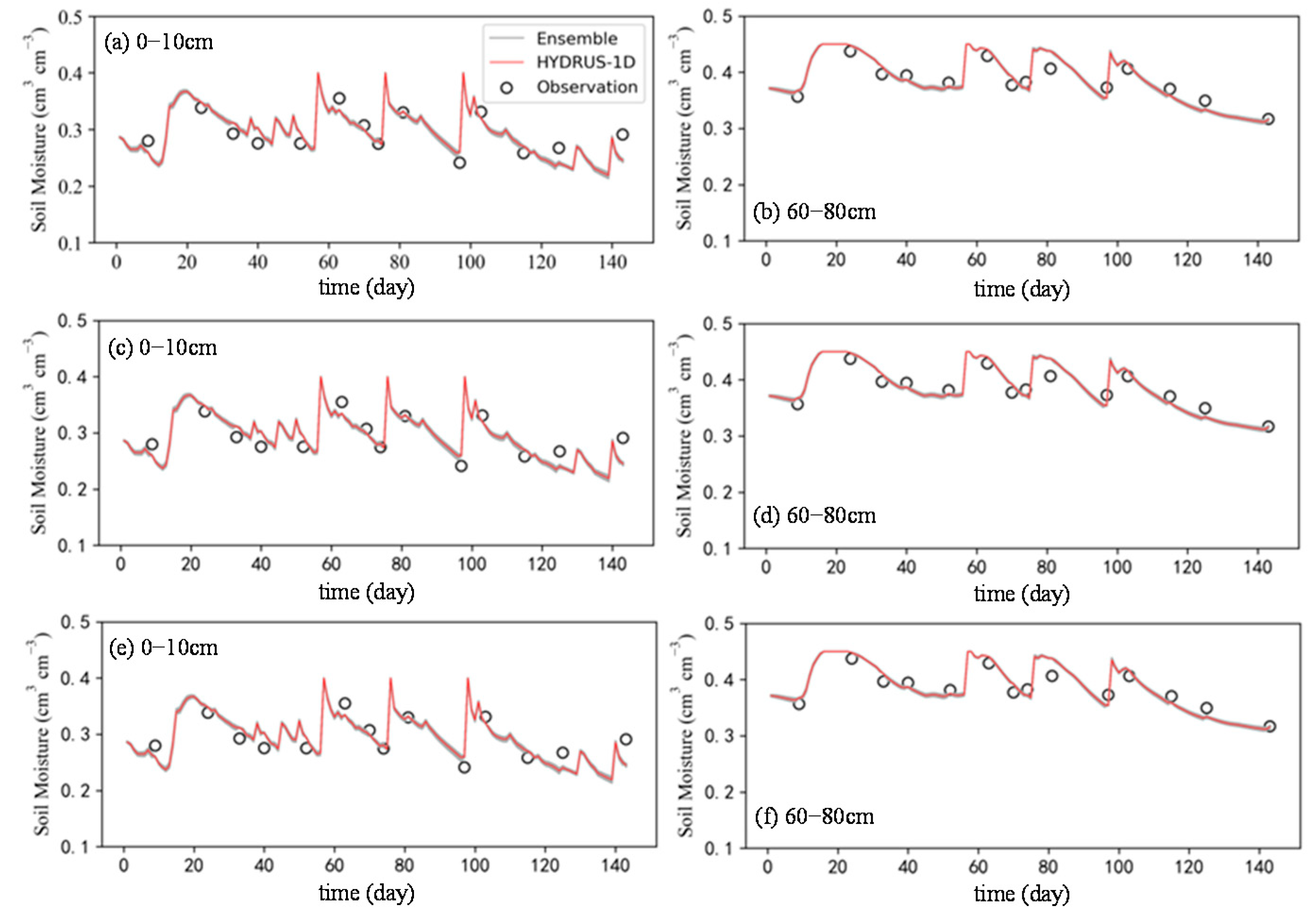
3.2. Water and Solute Dynamics Processes with Assimilation of Soil Moisture

The established assimilation system was applied to verify its practicability in field conditions. The reference parameter values used for assimilation listed in Table 1 were used with soil moisture data. Other model setups duplicate those in Section 2.4. Figure 3 and Figure 4 show the dynamics of the soil moisture and salinity, respectively, at different depths of the simulation. The green dashed lines labeled HYDRUS-1D in Figure 3 and Figure 4 represent the results simulated by Ren et al. [34]. Both nonlinear least squares estimation of parameters and trial and error curves fitting were employed in their simulation. The “assimilation” marked with solid red lines denotes results from the EnKF with parameter optimization. The assimilation results concur with the simulated results from HYDRUS-1D. Often, a limitation in assimilation times and a lack of observation data are the two most significant obstacles in the application of the EnKF for soil moisture and solute predictions. However, in our experiment, there appeared to be no distinguishing differences between the results of the EnKF and the least squares fitting when the number of assimilations approached 14, for both soil moisture and salinity.

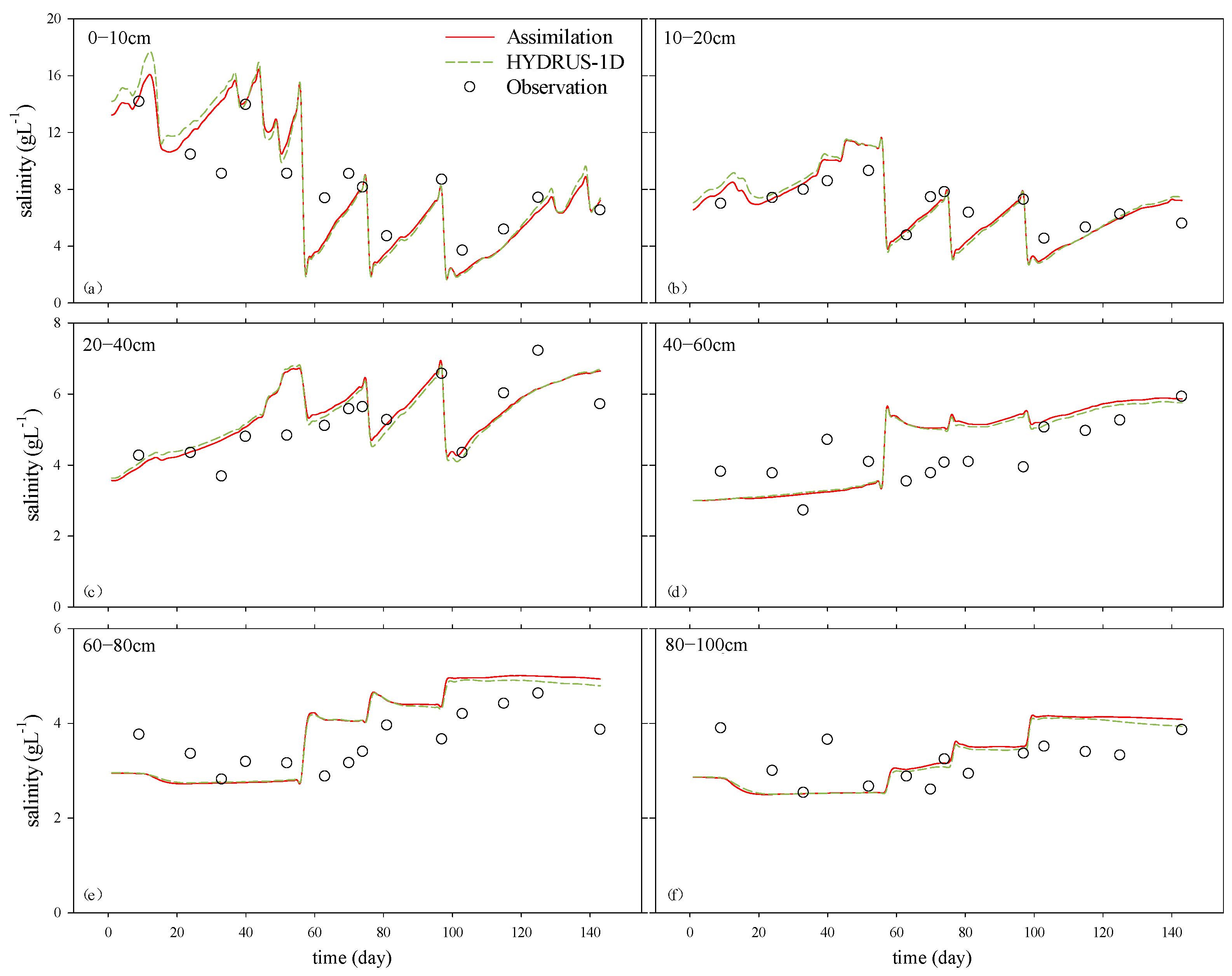
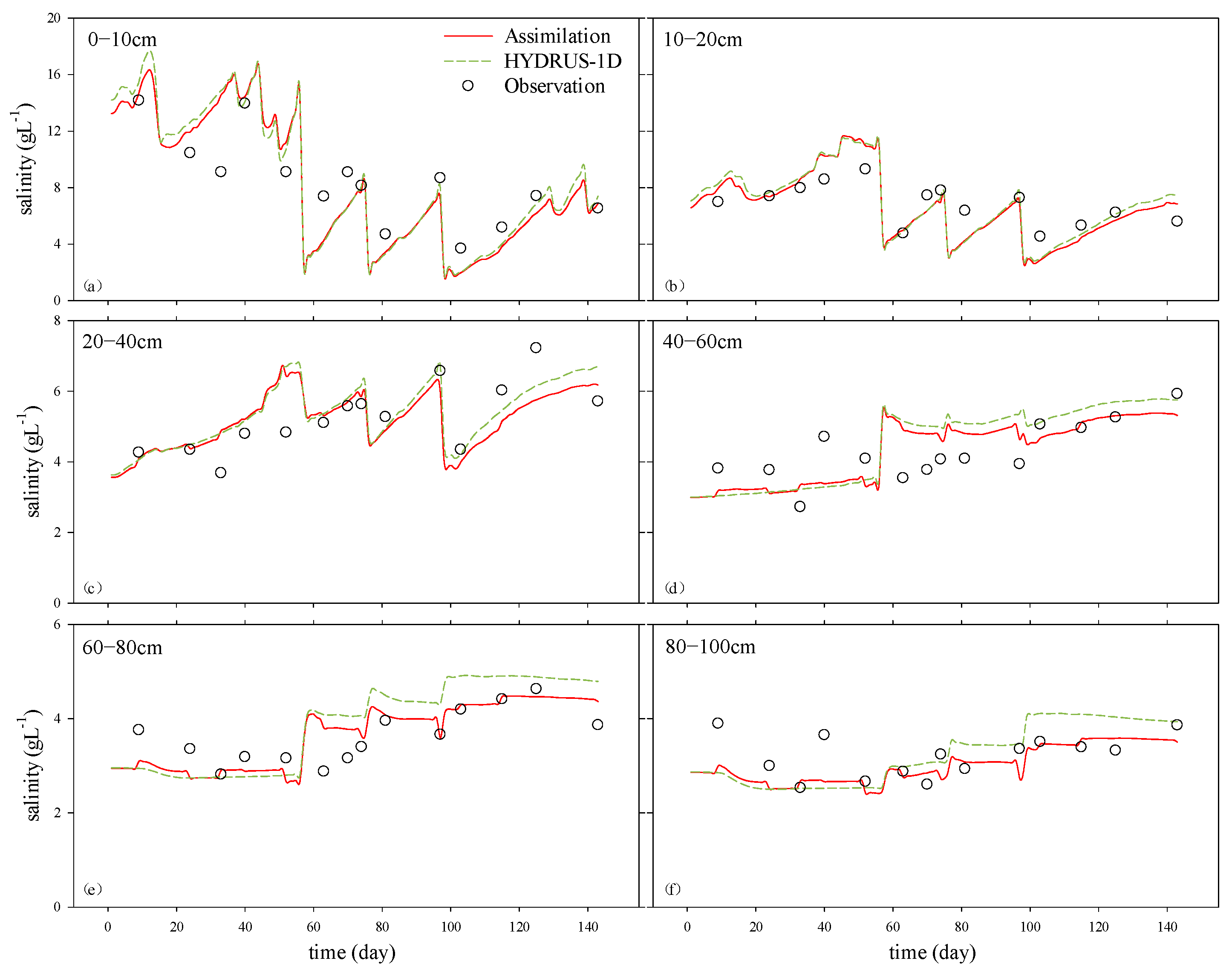
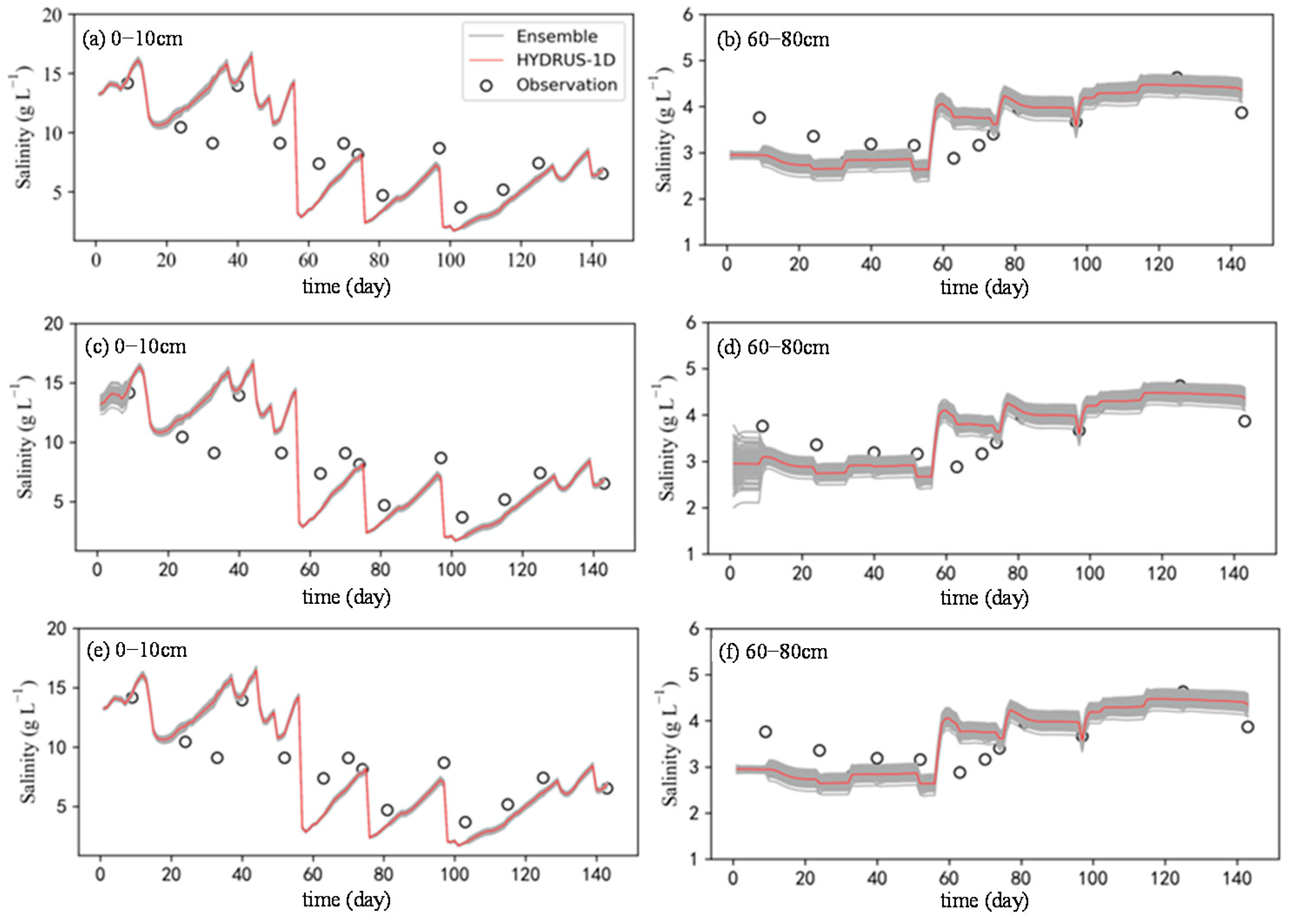
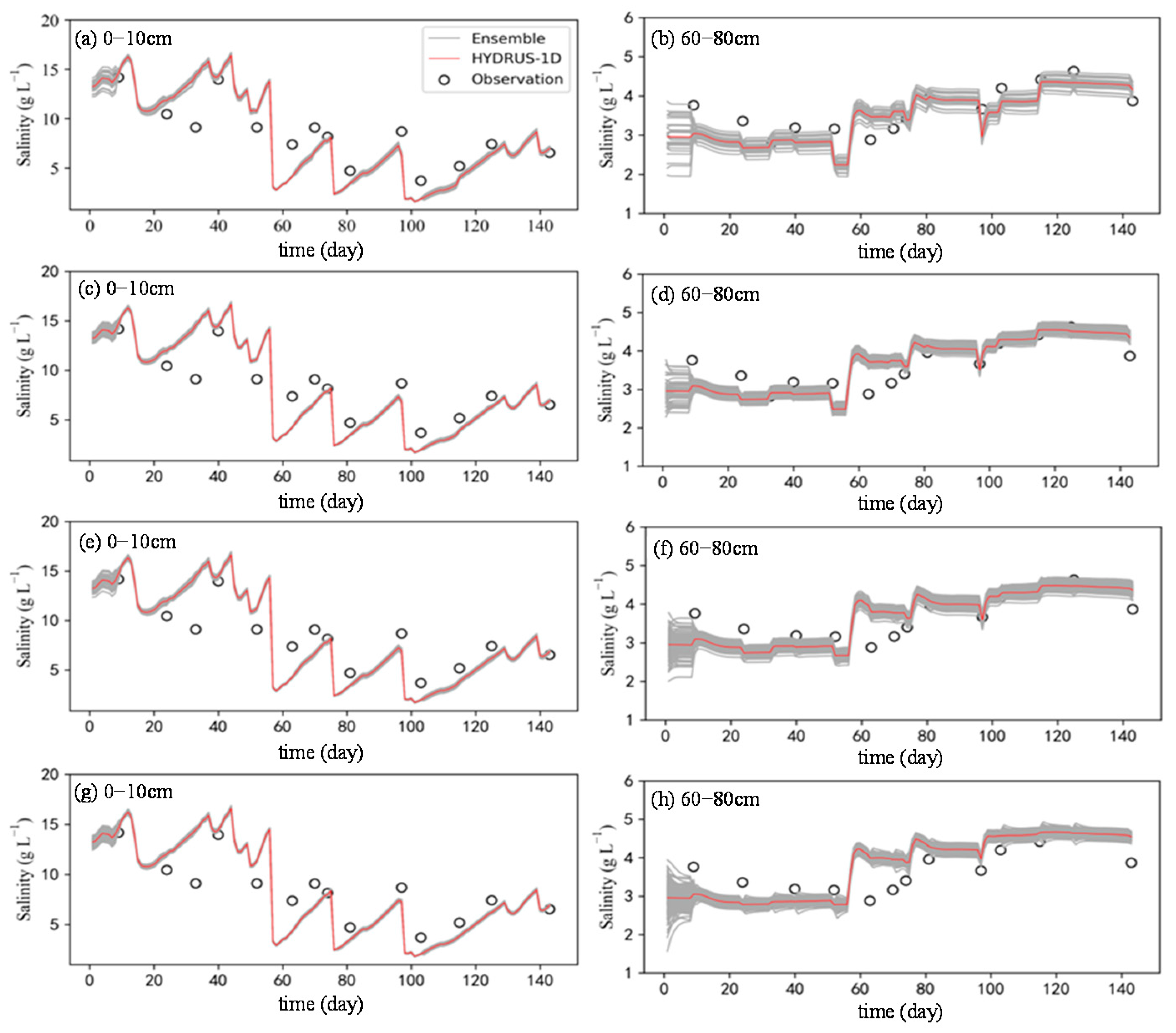
3.3. Water and Solute Dynamics Process for Assimilation of Soil Moisture, Salinity, and Parameters

Both the salinity data and the parameter L were considered in the assimilation process to investigate the parameter-estimation capability of the EnKF. The dynamic processes of soil moisture from observation, simulation, and assimilation at different depths are depicted in Figure 5, indicating a perfect match for the soil moisture among the three datasets. The results are even better than those for the assimilation shown in Figure 3 for a certain period. Figure 6 shows the measured, simulated, and assimilated soil salinity content at different depths. Compared with Figure 4, the simulation results for the soil salinity at different depths improved when the EnKF was applied. Both figures indicated better simulations for the salinity of deeper layers (e.g., below 40 cm) than for that of the surface layers. Furthermore, the simulated results for the salinity tended to be better at the later assimilation stage; for example, the simulated results for greater than 60 d were better than those for the days prior to day 60. Additionally, it appears that assimilating both the soil moisture and salinity did not significantly improve the prediction of the soil moisture; however, it improved the prediction of the salinity dynamics, particularly for the deeper layers.

The evolution of the estimated hydraulic conductivity (K_s), shape parameter (α), and longitudinal dispersivity (L) values are shown in Figure 7. The estimated results of K_s1 and K_s3 for unsaturated and saturated zones, respectively, were obviously stable during the assimilation process, and similar tendencies for α and L are also observed in Figure 7. The standard deviations of K_s1 and α₁ increased over time. The primary reason for the increase was the impact of the uncertainty on the upper boundary condition. The standard deviations of K_s3 and α₃ were stable during the simulation, and the standard deviations of L₁ and L₃ were stable during all simulation periods. Because of the insufficient measured data during assimilation, deviation from the true value usually occurs when the EnKF is applied for parameter estimation. Because the initial approximations for the parameters are used as the reference values in the assimilation, accurate results for parameter estimation cannot be achieved if significant differences exist between the initial estimations of the parameters and the true values.

Ren et al. [34] used the procedures of nonlinear least squares fitting in addition to the trial and error method to obtain optimized parameters, at the high cost of extensive human labor. The results of parameter estimation using the EnKF proved to be of similar quality to those of Ren et al. [34], although the procedures were both more straightforward and far less intensive with regard to human labor. Furthermore, the results for the assimilation of the salinity were improved compared with the original simulation results obtained by Ren et al. [34]. The goodness-of-fit indices for the simulation of the salinity are presented in

Table 4. Goodness-of-fit test indicators for simulations with the assimilation of soil salinity data.

Indicator	Original Simulation	Assimilating Soil Moisture	Assimilating Soil Moisture and Salinity
RMSE (cm3 cm−3)	1.191	1.113	1.116
MRE (%)	−3.345	−3.579	1.708
NSE	0.741	0.743	0.772
R2	0.822	0.830	0.834

. In the present study, the assimilation of L improved the simulation results compared with the MRE and NSE assimilation values for the original simulation. This indicates that assimilation with the estimation of L can yield better results than assimilation of only the salinity.

The RMSE values of the soil salinity were calculated for the entire simulation period, as shown in Figure 8. The RMSE values of the simulation results for the depth of 0–30 cm were slightly smaller than those of the original simulation, in which the parameter estimation for salinity dynamics was not considered. The RMSE values below 30 cm indicated that the original simulation was slightly better than the assimilation results. Furthermore, the parameter estimation improved the accuracy of the salinity prediction. The results of direct simulation via HYDRUS-1D were better than those of the assimilation result when the parameters for the salinity dynamics were considered for depth below 30 cm. In contrast, the assimilation results for the salinity were significantly improved compared with those of the original simulation when the parameter estimations were considered.

This study indicates that the EnKF is effective for handling the highly nonlinear dynamics of soil moisture and salinity, even for layered soil profiles. Figure 9 shows that both the soil moisture and salinity were accurately predicted via the EnKF scheme within the assimilating depths of 0–100 cm, although the prediction of the soil moisture was better than that of the salinity. Similar conclusions were reported by Wu and Margulis [26]. Onsite soil moisture and solution electrical conductivity (EC) data from sensors were used for data assimilation in their study. A far larger deviation was observed between the results of the assimilation and measurement in the study of Wu and Margulis than in the present study. The primary reason for the bias of the EnKF simulation was the uncertainties of the measurements from the sensor. High quality on-site measured data may improve the goodness-of-fit in the application of the EnKF method. Thus, the uncertainties of the data source are an important aspect worth considering in the application of the EnKF for hydrological modeling, particularly in cases where parameter estimation is required.

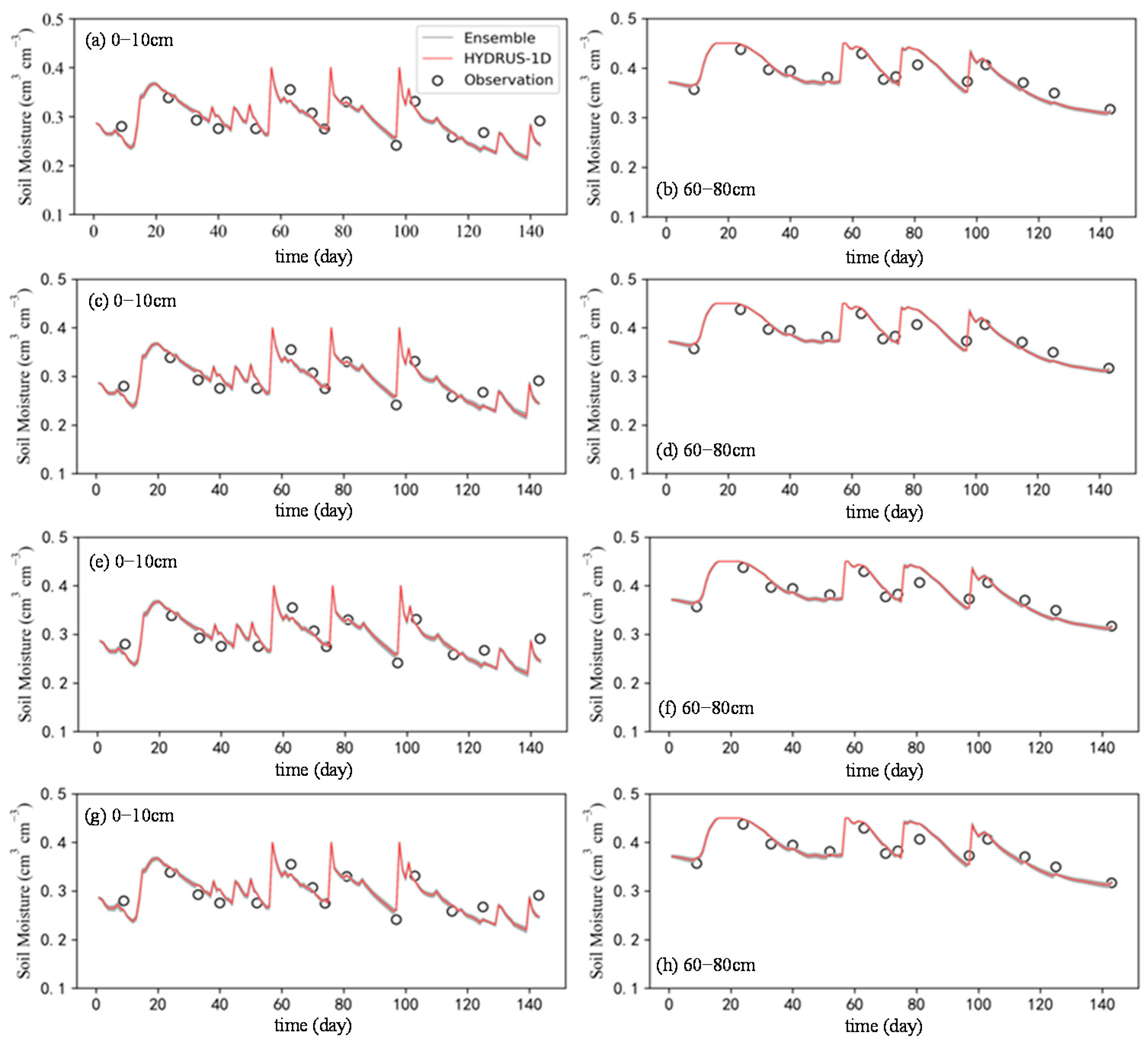
3.4. Impact of Initial Perturbation

To analyze the influence of the initial perturbation on the assimilation results, different standard deviations of the water content and salt concentration—(1) 0.001 cm³ cm⁻³, 0.1 g L⁻¹; (2) 0.001 cm³ cm⁻³, 1 g L⁻¹; and (3) 0.01 cm³ cm⁻³, 0.1 g L⁻¹—were applied in a numerical scheme. Figure 10 shows the soil moisture simulated using the EnKF at different initial perturbations. Figure 11 shows the simulated salinity concentration in the same situation as that of Figure 10. It appears that the initial perturbations had less effect on the results of the soil moisture simulation, while the initial perturbation of the salinity may have caused a significant bias in the results of salinity simulation. The remarkable bias of the simulated results could also cause divergence in certain cases or parts of the simulation period. If the parameter estimation process was stable, the impact of the initial perturbation decreased rapidly and remained stable after assimilation. The simulated soil moisture was not significantly influenced by the simulation results for the salinity. This may have been caused by the small standard deviation of the moisture.

3.5. Influence of Ensemble Size

Ensemble size significantly affected the assimilation results in for the EnKF method and thus also influenced the simulated results for the soil moisture and salinity. Different ensemble sizes—(1) 30, (2) 50, (3) 100, and (4) 200—were adopted to investigate the effects of the ensemble size on the assimilation processes and simulation results. Because the quality of parameter estimation is affected greatly by the quantity of field observation data, the influence of the ensemble size on the parameter estimation will not be discussed in this section, as limited field observation data were employed in the numerical scheme. According to Figure 12, we concluded that the ensemble size had little influence on the soil moisture at different depths, indicating that a reasonable or relatively small initial perturbation was given for the soil moisture. Figure 13 shows the effect of the ensemble size on the assimilation of the salinity for different soil depths. Clearly, the estimated results for the salinity were strongly influenced by the ensemble size compared with the soil moisture. A smaller ensemble size yielded a broader distribution of the simulated salinity values. Thus, a reasonably large ensemble size (e.g., 50 to 100) can be useful for obtaining a stable assimilation result when the EnKF is applied in highly nonlinear hydrological models.

4. Discussion

As mentioned previously, the quality of parameter estimation via the EnKF for nonlinear hydrological models is subject to two major constraints: uncertainties in the data source and the quantity of observations. It is difficult to obtain an accurate result with uncertain data or sparse observations in either the spatial or temporal scale. In our study, sampling data from six different layers with soil depths of 0–100 cm were used for assimilation. The simulated soil profile spanned depths of 0–300 cm, which could include substantial differences in the soil texture, as well as in the parameters for water and solute transport. Nodes far from the observation points exhibited weaker correlations to the observation points, which may cause inaccurate estimation of parameters and prediction of state variables when the EnKF method is applied. A numerical experiment was performed setting the initial estimates of parameters to the true values to validate the simulation. The parameter estimation and state prediction were improved by reducing the depth of the simulation or the number of grids for spatial discretization. However, there was a need to balance these two factors and balance the EnKF with the model operator. In this study, reducing the number of grids for spatial discretization compromised the numerical stability of HYDRUS-1D. Furthermore, sparse observation data of field conditions was common, which influenced the assimilation accuracy. Compared with the application of Wu and Margulis [26], this study had the benefit of less uncertainties in the measured data. This is because Wu and Margulis [26] obtained measurements using an onsite sensor, while we acquired our data through soil sampling. Thus, accurate measurement of the state variables can mitigate an insufficient dataset when used for assimilation.

In this study, the assimilation results for the soil moisture and salinity appeared to be independent, which contradicts the fact that salinity dynamics depend on water movement. The main reason for this result may be that the assimilations of the soil moisture and salinity were conducted separately in the HYDRUS-1D model, and the calculation of the solute transport was based on the water-movement results. In HYDRUS-1D, the water movement was simulated via sequential iteration untill the threshold for the water content/pressure was satisfied for a certain timestep. Then, the pore velocity of water was used to simulate the solute transport via another sequential iteration untill the threshold for the solute concentration was satisfied for the same timestep. Thus, the water movement and salinity transport were modeled separately for a certain timestep. In contrast to HYDRUS-1D, which is physical process-based model, the EnKF is a statistical method. It is impossible for the EnKF to allocate reasonable weights for the soil moisture, salinity, and parameters of solute transport during parameter estimation for the dynamics of the soil moisture process. Thus, further investigation of simultaneously solving the water and solute movement is needed to improve the assimilation results when the EnKF is applied to layered, variably saturated soil profiles.

The uncertainty in the upper boundary condition could also have an important impact on the parameter estimation and hydrologic simulations. Factors, such as the weather conditions (precipitation, potential evapotranspiration, etc.), irrigation practices, crop-growth conditions (amount and location of water abstraction from the root zone, real evapotranspiration, etc.), that were applied in the simulation may have deviated from the onsite field conditions. This type of uncertainty could have significantly affected the upper layer when the assimilation was implemented (as shown in Figure 7). Although proper quantification of the uncertainty on the upper boundary condition can improve the simulation results, further investigation is needed for higher efficiency and more robust assimilation when the EnKF is in combined with HYDRUS-1D.

5. Conclusions

The EnKF has been proven to be an effective tool for data assimilation in diverse areas. In this study, data from a field experiment in the Hetao Irrigation District were used to investigate the performance of the EnKF in combination with the HYDRUS-1D model under field conditions. Numerical schemes, including diverse perturbation for initial values, different ensemble sizes, and parameter estimation, were considered. The results and conclusions are as follows.

• The EnKF effectively estimates parameters and predicts state variables such as the soil moisture and salinity in layered, variably saturated soils when used with HYDRUS-1D. The reliability of the results was highly dependent on the proper selection of assimilating factors such as initial perturbation and ensemble size. A reasonable ensemble size range of 50–100 yields stable assimilation results when the EnKF is applied to highly nonlinear hydrological models such as that of this study.
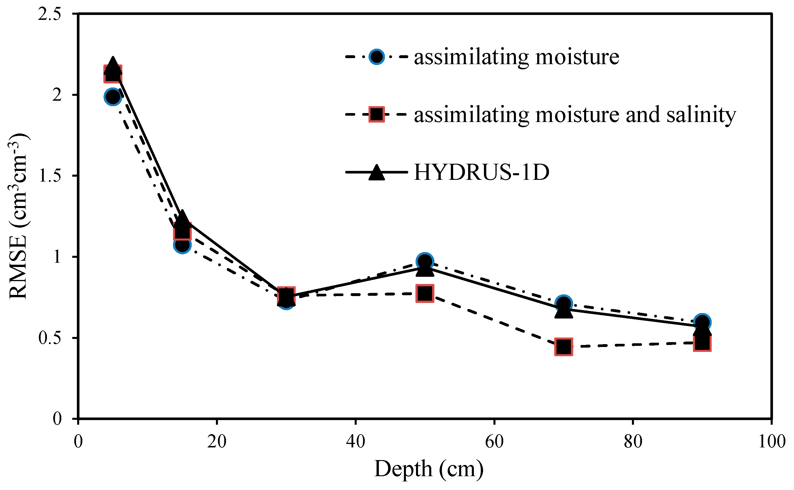
• The simulation results for moisture could not be significantly improved through the assimilation of the soil moisture and relative parameters, but the simulation of the salinity was significantly improved through the assimilation of the salinity and relative solute-transport parameters.
• The bias of the EnKF simulation was primarily attributed to the uncertainties of the measurements from the sensor. High-quality onsite measured data improved the goodness-of-fit when the EnKF method was applied. Thus, the uncertainties of the data source are an important aspect to consider when the EnKF is applied to hydrological modeling, particularly when parameter estimation is required. Sparse observation data of field conditions benefits from the accurate measurement of states variables in the application of EnKF assimilation.

The application of the EnKF algorithm for layered, variably saturated soils with a hydrological model requires additional study, because solving the inherent physical model of the van Genuchten–Mualem equation is a highly nonlinear problem and the situation is further complicated in cases of sophisticated boundary conditions and a detailed driving force.

References

1. Vrugt, J.A.; Schoups, G.; Hopmans, J.W.; Young, C.; Wallender, W.W.; Harter, T.; Bouten, W. Inverse modeling of large-scale spatially distributed vadose zone properties using global optimization. Water Resour. Res. 2004, 40, 308–322. [Google Scholar] [CrossRef]
2. Wood, A.W.; Lettenmaier, D.P. An ensemble approach for attribution of hydrologic prediction uncertainty. Geophys. Res. Lett. 2008, 35. [Google Scholar] [CrossRef] [Green Version]
3. Le Bourgeois, O.; Bouvier, C.; Brunet, P.; Ayral, P.A. Inverse modeling of soil water content to estimate the hydraulic properties of a shallow soil and the associated weathered bedrock. J. Hydrol. 2016, 541, 116–126. [Google Scholar] [CrossRef]
4. Pan, F.; McKane, R.B.; Stieglitz, M. Identification of optimal soil hydraulic functions and parameters for predicting soil moisture. Hydrol. Sci. J. 2012, 57, 723–737. [Google Scholar] [CrossRef] [Green Version]
5. Gharamti, M.; Ait-El-Fquih, B.; Hoteit, I. An iterative ensemble Kalman filter with one-step-ahead smoothing for state-parameters estimation of contaminant transport models. J. Hydrol. 2015, 527, 442–457. [Google Scholar] [CrossRef] [Green Version]
6. Pan, L.; Wu, L. A hybrid global optimization method for inverse estimation of hydraulic parameters: Annealing-Simplex Method. Water Resour. Res. 1998, 34, 2261–2269. [Google Scholar] [CrossRef]
7. Takeshita, Y.; Nakazawa, K.; Fukuda, D.; Kohno, I. Determination of unsaturated soil hydraulic properties from transient outflow experiments using genetic algorithms. Doboku Gakkai Ronbunshu 1999, 191–201. [Google Scholar] [CrossRef]
8. Javaux, M.; Hupet, F.; Lambot, S.; Vanclooster, M. A global multilevel coordinate search procedure for estimating the unsaturated soil hydraulic properties. Water Resour. Res. 2002, 38, 6-1–6-15. [Google Scholar]
9. Abbaspour, K.; Schulin, R.; Van Genuchten, M.; Van Genuchten, M. Estimating unsaturated soil hydraulic parameters using ant colony optimization. Adv. Water Resour. 2001, 24, 827–841. [Google Scholar] [CrossRef]
10. Mertens, J.; Madsen, H.; Kristensen, M.; Jacques, D.; Feyen, J. Sensitivity of soil parameters in unsaturated zone modelling and the relation between effective, laboratory and in situ estimates. Hydrol. Process. 2005, 19, 1611–1633. [Google Scholar] [CrossRef]
11. Schoups, G.; Hopmans, J.; Young, C.; Vrugt, J.; Wallender, W. Multi-criteria optimization of a regional spatially-distributed subsurface water flow model. J. Hydrol. 2005, 311, 20–48. [Google Scholar] [CrossRef]
12. Vrugt, J.A.; Robinson, B.A. Improved evolutionary optimization from genetically adaptive multimethod search. Proc. Natl. Acad. Sci. USA 2007, 104, 708–711. [Google Scholar] [CrossRef] [PubMed] [Green Version]
13. Vrugt, J.A.; Stauffer, P.H.; Wöhling, T.; Robinson, B.A.; Vesselinov, V.V. Inverse Modeling of Subsurface Flow and Transport Properties: A Review with New Developments. Vadose Zone J. 2008, 7, 843. [Google Scholar] [CrossRef]
14. Evensen, G. Sequential data assimilation with a nonlinear quasi-geostrophic model using Monte Carlo methods to forecast error statistics. J. Geophys. Res. Space Phys. 1994, 99, 10143. [Google Scholar] [CrossRef]
15. Entekhabi, D.; Dunne, S.; Margulis, S.A.; McLaughlin, D. Land data assimilation and estimation of soil moisture using measurements from the Southern Great Plains 1997 Field Experiment. Water Resour. Res. 2002, 38, 1299. [Google Scholar]
16. Das, N.N.; Mohanty, B.P. Root Zone Soil Moisture Assessment Using Remote Sensing and Vadose Zone Modeling. Vadose Zone J. 2006, 5, 296. [Google Scholar] [CrossRef]
17. Huang, C.; Hu, B.X.; Li, X.; Ye, M. Using data assimilation method to calibrate a heterogeneous conductivity field and improve solute transport prediction with an unknown contamination source. Stoch. Env. Res. Risk A 2009, 23, 1155–1167. [Google Scholar] [CrossRef]
18. Xie, X.; Zhang, D. Data assimilation for distributed hydrological catchment modeling via ensemble Kalman filter. Adv. Water Resour. 2010, 33, 678–690. [Google Scholar] [CrossRef]
19. Li, L.; Zhou, H.; Franssen, H.J.H.; Gómez-Hernández, J.J.; Gómez-Hernández, J.J.; Gómez-Hernández, J.J. Modeling transient groundwater flow by coupling ensemble Kalman filtering and upscaling. Water Resour. Res. 2012, 48. [Google Scholar] [CrossRef] [Green Version]
20. Wanders, N.; Karssenberg, D.; De Roo, A.; De Jong, S.; Bierkens, M.F.P. The suitability of remotely sensed soil moisture for improving operational flood forecasting. Hydrol. Earth Syst. Sci. 2014, 18, 2343–2357. [Google Scholar] [CrossRef] [Green Version]
21. Zhang, H.; Kurtz, W.; Kollet, S.; Vereecken, H.; Franssen, H.J.H. Comparison of different assimilation methodologies of groundwater levels to improve predictions of root zone soil moisture with an integrated terrestrial system model. Adv. Water Resour. 2018, 111, 224–238. [Google Scholar] [CrossRef]
22. Vrugt, J.A.; Diks, C.G.H.; Gupta, H.V.; Bouten, W.; Verstraten, J.M. Improved treatment of uncertainty in hydrologic modeling: Combining the strengths of global optimization and data assimilation. Water Resour. Res. 2005, 41, 1–17. [Google Scholar] [CrossRef]
23. Chen, Y.; Zhang, D. Data assimilation for transient flow in geologic formations via ensemble Kalman filter. Adv. Water Resour. 2006, 29, 1107–1122. [Google Scholar] [CrossRef]
24. Franssen, H.J.H.; Kaiser, H.P.; Kuhlmann, U.; Bauser, G.; Stauffer, F.; Muller, R.; Kinzelbach, W. Operational real-time modeling with ensemble Kalman filter of variably saturated subsurface flow including stream-aquifer interaction and parameter updating. Water Resour. Res. 2011, 47. [Google Scholar] [CrossRef]
25. Man, J.; Zheng, Q.; Wu, L.; Zeng, L. Improving parameter estimation with an efficient sequential probabilistic collocation-based optimal design method. J. Hydrol. 2019, 569, 1–11. [Google Scholar] [CrossRef]
26. Wu, C.C.; Margulis, S.A. Real-Time Soil Moisture and Salinity Profile Estimation Using Assimilation of Embedded Sensor Datastreams. Vadose Zone J. 2013, 12. [Google Scholar] [CrossRef]
27. Li, C.; Ren, L. Estimation of Unsaturated Soil Hydraulic Parameters Using the Ensemble Kalman Filter. Vadose Zone J. 2011, 10, 1205–1227. [Google Scholar] [CrossRef]
28. Song, X.; Shi, L.; Ye, M.; Yang, J.; Navon, I.M. Numerical Comparison of Iterative Ensemble Kalman Filters for Unsaturated Flow Inverse Modeling. Vadose Zone J. 2014, 13. [Google Scholar] [CrossRef]
29. Gharamti, M.; Valstar, J.; Hoteit, I. An adaptive hybrid EnKF-OI scheme for efficient state-parameter estimation of reactive contaminant transport models. Adv. Water Resour. 2014, 71, 1–15. [Google Scholar] [CrossRef]
30. Šimůnek, J.; Šejna, M.; Saito, H. The HYDRUS-1D Software Package for Simulating the Movement of Water, Heat, and Multiple Solutes in Variably-Saturated Media, version 4.08; HYDRUS Software Series 3; Department of Environmental Sciences, University of California Riverside: Riverside, CA, USA, 2009; p. 315. [Google Scholar]
31. Van Genuchten, M.T. A closed-form equation for predicting the hydraulic conductivity of unsaturated soils. Soil Sci. Soc. Am. 1980, 5, 892–898. [Google Scholar] [CrossRef]
32. Mualem, Y. A new model for predicting the hydraulic conductivity of unsaturated porous media. Water Resour. Res. 1976, 12, 513–522. [Google Scholar] [CrossRef] [Green Version]
33. Evensen, G. The Ensemble Kalman Filter: Theoretical formulation and practical implementation. Ocean. Dyn. 2003, 53, 343–367. [Google Scholar] [CrossRef]
34. Ren, D.; Xu, X.; Hao, Y.; Huang, G. Modeling and assessing field irrigation water use in a canal system of Hetao, upper Yellow River basin: Application to maize, sunflower and watermelon. J. Hydrol. 2016, 532, 122–139. [Google Scholar] [CrossRef]
35. LeGates, D.R.; McCabe, G.J. Evaluating the use of “goodness-of-fit” Measures in hydrologic and hydroclimatic model validation. Water Resour. Res. 1999, 35, 233–241. [Google Scholar] [CrossRef]
36. Moriasi, D.N.; Arnold, J.G.; Van Liew, M.W.; Bingner, R.L.; Harmel, R.D.; Veith, T.L. Model Evaluation Guidelines for Systematic Quantification of Accuracy in Watershed Simulations. Trans. ASABE 2007, 50, 885–900. [Google Scholar] [CrossRef]
37. Nash, J.; Sutcliffe, J. River flow forecasting through conceptual models part I—A discussion of principles. J. Hydrol. 1970, 10, 282–290. [Google Scholar] [CrossRef]
Figure 1. Flowchart of data assimilation for soil water movement and solute transport using the EnKF coupled with HYDRUS-1D.
Water 11 01520 g001
Figure 2. Evolution of the estimated hydraulic conductivity (Ks), shape parameter (α), and longitudinal dispersivity (L) values using EnKF.
Water 11 01520 g002
Figure 3. Simulated soil moisture at different depths with assimilation of only the soil moisture. (Green dashed lines represent the simulated results from Ren et al. [34] obtained using HYDRUS-1D; red solid lines represent the assimilation results).
Water 11 01520 g003
Figure 4. Simulated salinity at different depths with assimilation of only the soil moisture. (Green dashed lines represent the simulated results from Ren et al. [34] obtained using HYDRUS-1D; red solid lines represent the assimilation results).
Water 11 01520 g004
Figure 5. Simulated soil moisture at different depths with assimilation of the soil moisture and salinity. (Green dashed lines represent the simulated results from Ren et al. [34] obtained using HYDRUS-1D; red solid lines represent the assimilation results).
Water 11 01520 g005
Figure 6. Simulated salinity at different depths with assimilation of the soil moisture and salinity. (Green dashed lines represent the simulated results from Ren et al. [34] obtained using HYDRUS-1D; red solid lines represent the assimilation results).
Water 11 01520 g006
Figure 7. Evolution of the estimated hydraulic conductivity (Ks), shape parameter (α), and longitudinal dispersivity (L) values with assimilation of the soil moisture and salinity.
Water 11 01520 g007
Figure 8. Comparison of the RMSE values for different depths in HYDRUS-1D, for the assimilation of only soil moisture and the assimilation of soil moisture and salinity.
Water 11 01520 g008
Figure 9. Sampling measurements versus EnKF estimates for soil with depths of 0–100 cm: (a) moisture; (b) salinity. The black circles represent the ensemble mean versus measurements at different time steps, and the solid black 1:1 diagonal line represents a perfect prediction.
Water 11 01520 g009
Figure 10. Simulated soil moisture at different depths with different initial perturbations of the soil moisture and salinity: (a) 0–10 cm, with standard deviations of 0.001 cm3 cm−3 for moisture and 0.1 g L−1 for salinity; (b) 60–80 cm, with standard deviations of 0.001 cm3 cm−3 for moisture and 0.1 g L−1 for salinity; (c) 0–10 cm, with standard deviations of 0.001 cm3 cm−3 for moisture and 1 g L−1 for salinity; (d) 60–80 cm, with standard deviations of 0.001 cm3 cm−3 for moisture and 1 g L−1 for salinity; (e) 0–10 cm, with standard deviations of 0.01 cm3 cm−3 for moisture and 0.1 g L−1 for salinity; (f) 60–80 cm, with standard deviations of 0.01 cm3 cm−3 for moisture and 0.1 g L−1 for salinity.
Water 11 01520 g010
Figure 11. Simulated salinity at different depths with different initial perturbations of the soil moisture and salinity: (a) 0–10 cm, with standard deviations of 0.001 cm3 cm−3 for moisture and 0.1 g L−1 for salinity; (b) 60–80 cm, with standard deviations of 0.001 cm3 cm−3 for moisture and 0.1 g L−1 for salinity; (c) 0–10 cm, with standard deviations of 0.001 cm3 cm−3 for moisture and 1 g L−1 for salinity; (d) 60–80 cm, with standard deviations of 0.001 cm3 cm−3 for moisture and 1 g L−1 for salinity; (e) 0–10 cm, with standard deviations of 0.01 cm3 cm−3 for moisture and 0.1 g L−1 for salinity; (f) 60–80 cm, with standard deviations of 0.01 cm3 cm−3 for moisture and 0.1 g L−1 for salinity.
Water 11 01520 g011
Figure 12. Simulated soil moisture at different depths with different ensemble sizes: (a) 0–10 cm, with an ensemble size of 30; (b) 60–80 cm, with an ensemble size of 30; (c) 0–10 cm, with an ensemble size of 50; (d) 60–80 cm, with an ensemble size of 50; (e) 0–10 cm, with an ensemble size of 100; (f) 60–80 cm, with an ensemble size of 100; (g) 0–10 cm, with an ensemble size of 200; (h) 60–80 cm, with an ensemble size of 200.
Water 11 01520 g012
Figure 13. Simulated salinity at different depths with different ensemble sizes, (a) 0–10 cm, with an ensemble size of 30; (b) 60–80 cm, with an ensemble size of 30; (c) 0–10 cm, with an ensemble size of 50; (d) 60–80 cm, with an ensemble size of 50; (e) 0–10 cm, with an ensemble size of 100; (f) 60–80 cm, with an ensemble size of 100; (g) 0–10 cm, with an ensemble size of 200; (h) 60–80 cm, with an ensemble size of 200.
Water 11 01520 g013