Integral Flow Modelling Approach for Surface Water-Groundwater Interactions along a Rippled Streambed

 and
and
Abstract
:1. Introduction
2. Materials and Methods
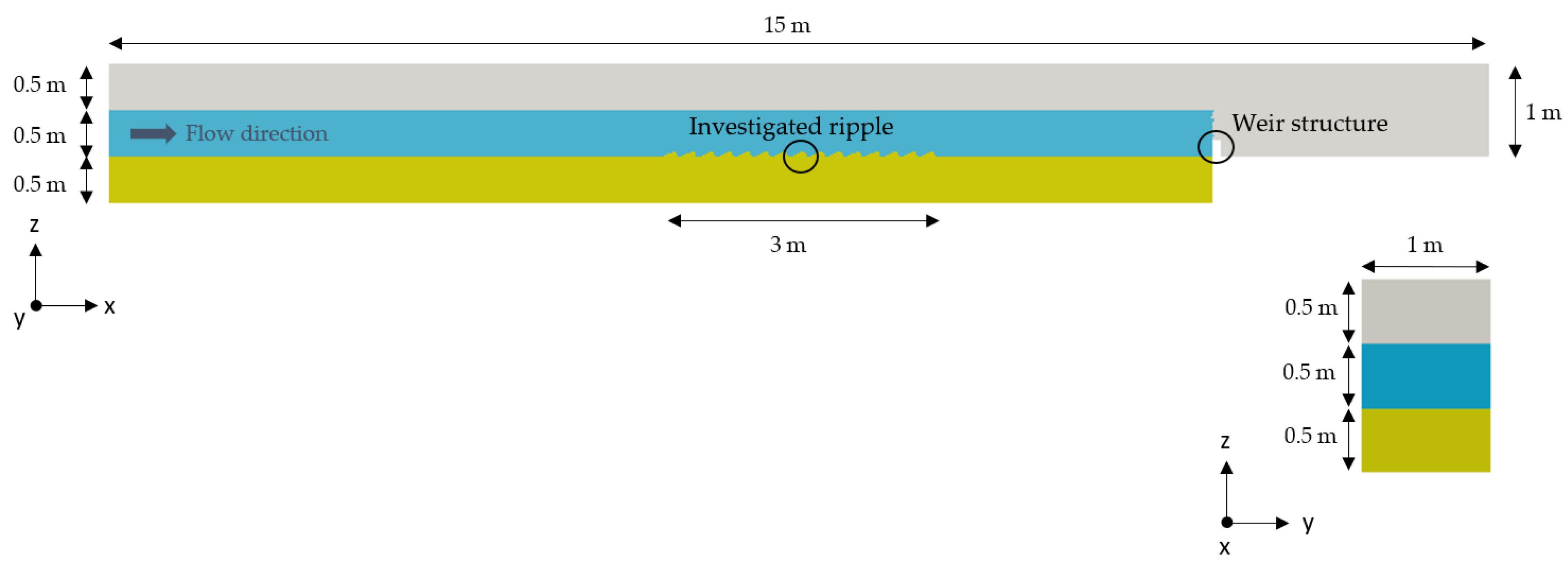
2.1. Geometry and Mesh
2.2. Numerical Model
2.3. Turbulence
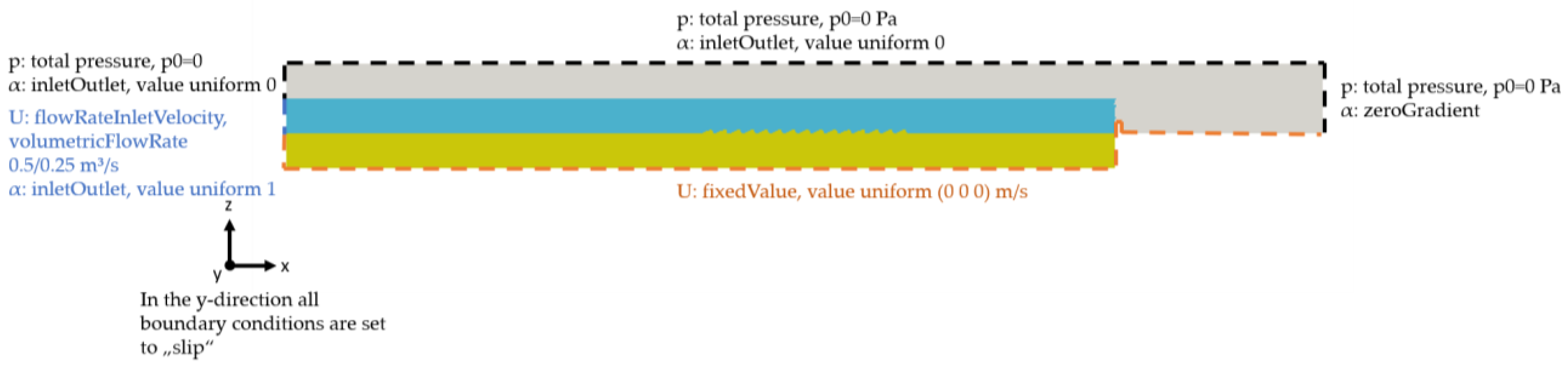
2.4. Boundary and Initial Conditions
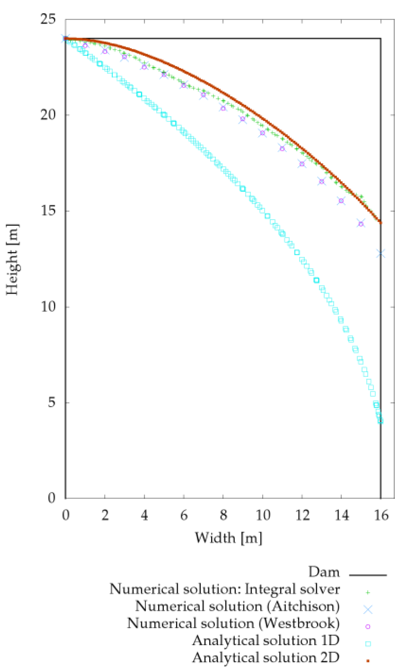
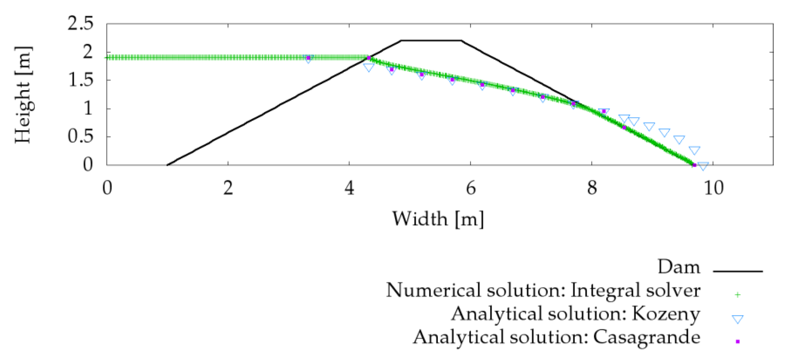
2.5. Validation
3. Results and Discussion
3.1. Reference Case
3.2. Ripple Dimension
3.3. Ripple Length
3.4. Ripple Distance
3.5. Flow Rate
4. Conclusions
Author Contributions
Funding
Acknowledgments
Conflicts of Interest
References
- Boulton, A.J.; Findlay, S.; Marmonier, P.; Stanley, E.H.; Valett, H.M. The functional significance of the hyporheic zone in streams and rivers. Annu. Rev. Ecol. Syst. 1998, 29, 59–81. [Google Scholar] [CrossRef]
- Brunke, M.; Gonser, T. The ecological significance of exchange processes between rivers and groundwater. Freshw. Biol. 1997, 37, 1–33. [Google Scholar] [CrossRef] [Green Version]
- Cardenas, M.B. Hyporheic zone hydrologic science: A historical account of its emergence and a prospectus. Water Resour. Res. 2015, 51, 3601–3616. [Google Scholar] [CrossRef]
- Dahm, C.N.; Grimm, N.B.; Marmonier, P.; Valett, H.M.; Vervier, P. Nutrient dynamics at the interface between surface waters and groundwaters. Freshw. Biol. 1998, 40, 427–451. [Google Scholar] [CrossRef]
- Findlay, S. Importance of surface-subsurface exchange in stream ecosystems: The hyporheic zone. Limnol. Oceanogr. 1995, 40, 159–164. [Google Scholar] [CrossRef]
- Gomez-Velez, J.D.; Harvey, J.W.; Cardenas, M.B.; Kiel, B. Denitrification in the Mississippi River network controlled by flow through river bedforms. Nat. Geosci. 2015, 8, 941. [Google Scholar] [CrossRef]
- Harvey, J.; Gooseff, M. River corridor science: Hydrologic exchange and ecological consequences from bedforms to basins. Water Resour. Res. 2015, 51, 6893–6922. [Google Scholar] [CrossRef] [Green Version]
- Stonedahl, S.H.; Harvey, J.W.; Packman, A.I. Interactions between hyporheic flow produced by stream meanders, bars, and dunes. Water Resour. Res. 2013, 49, 5450–5461. [Google Scholar] [CrossRef]
- Stonedahl, S.H.; Harvey, J.W.; Wörman, A.; Salehin, M.; Packman, A.I. A multiscale model for integrating hyporheic exchange from ripples to meanders. Water Resour. Res. 2010, 46. [Google Scholar] [CrossRef] [Green Version]
- Schaper, J.L.; Posselt, M.; McCallum, J.L.; Banks, E.W.; Hoehne, A.; Meinikmann, K.; Shanafield, M.A.; Batelaan, O.; Lewandowski, J. Hyporheic Exchange Controls Fate of Trace Organic Compounds in an Urban Stream. Environ. Sci. Technol. 2018, 52, 12285–12294. [Google Scholar] [CrossRef] [Green Version]
- Harvey, J.W.; Bencala, K.E. The Effect of streambed topography on surface-subsurface water exchange in mountain catchments. Water Resour. Res. 1993, 29, 89–98. [Google Scholar] [CrossRef]
- Winter, T.C.; Harvey, J.W.; Franke, O.L.; Alley, W.M. Ground Water and Surface Water; a Single Resource; Diane Publishing Inc.: Darby, PA, USA, 1998; Volume 1139. [Google Scholar]
- Wondzell, S.M.; Gooseff, M. Geomorphic controls on hyporheic exchange across scales: Watersheds to particles. Treatise Geomorphol. 2013, 9, 203–218. [Google Scholar]
- Elliott, A.H.; Brooks, N.H. Transfer of nonsorbing solutes to a streambed with bed forms: Laboratory experiments. Water Resour. Res. 1997, 33, 137–151. [Google Scholar] [CrossRef]
- Packman, A.I.; Salehin, M.; Zaramella, M. Hyporheic Exchange with Gravel Beds: Basic Hydrodynamic Interactions and Bedform-Induced Advective Flows. J. Hydraul. Eng. 2004, 130, 647–656. [Google Scholar] [CrossRef]
- Mutz, M.; Kalbus, E.; Meinecke, S. Effect of instream wood on vertical water flux in low-energy sand bed flume experiments. Water Resour. Res. 2007, 43. [Google Scholar] [CrossRef]
- Tonina, D.; Buffington, J.M. Hyporheic exchange in gravel bed rivers with pool-riffle morphology: Laboratory experiments and three-dimensional modeling. Water Resour. Res. 2007, 43. [Google Scholar] [CrossRef] [Green Version]
- Tonina, D.; Buffington, J.M. A three-dimensional model for analyzing the effects of salmon redds on hyporheic exchange and egg pocket habitat. Can. J. Fish. Aquat. Sci. 2009, 66, 2157–2173. [Google Scholar] [CrossRef] [Green Version]
- Voermans, J.; Ghisalberti, M.; Ivey, G. The variation of flow and turbulence across the sediment–water interface. J. Fluid Mech. 2017, 824, 413–437. [Google Scholar] [CrossRef]
- Saenger, N.; Kitanidis, K.P.; Street, R. A numerical study of surface-subsurface exchange processes at a riffle-pool pair in the Lahn River, Germany. Water Resour. Res. 2005, 41, 12424. [Google Scholar] [CrossRef]
- Cardenas, M.B.; Wilson, J.L. Dunes, turbulent eddies, and interfacial exchange with permeable sediments. Water Resour. Res. 2007, 43. [Google Scholar] [CrossRef]
- Bardini, L.; Boano, F.; Cardenas, M.B.; Revelli, R.; Ridolfi, L. Nutrient cycling in bedform induced hyporheic zones. Geochim. Cosmochim. Acta 2012, 84, 47–61. [Google Scholar] [CrossRef] [Green Version]
- Trauth, N.; Schmidt, C.; Maier, U.; Vieweg, M.; Fleckenstein, J.H. Coupled 3-D stream flow and hyporheic flow model under varying stream and ambient groundwater flow conditions in a pool-riffle system. Water Resour. Res. 2013, 49, 5834–5850. [Google Scholar] [CrossRef]
- Trauth, N.; Schmidt, C.; Vieweg, M.; Maier, U.; Fleckenstein, J.H. Hyporheic transport and biogeochemical reactions in pool-riffle systems under varying ambient groundwater flow conditions. J. Geophys. Res. Biogeosci. 2014, 119, 910–928. [Google Scholar] [CrossRef]
- Chen, X.; Cardenas, M.B.; Chen, L. Hyporheic Exchange Driven by Three-Dimensional Sandy Bed Forms: Sensitivity to and Prediction from Bed Form Geometry. Water Resour. Res. 2018, 54, 4131–4149. [Google Scholar] [CrossRef]
- Chen, X.; Cardenas, M.B.; Chen, L. Three-dimensional versus two-dimensional bed form-induced hyporheic exchange. Water Resour. Res. 2015, 51, 2923–2936. [Google Scholar] [CrossRef]
- VanderKwaak, J.E. Numerical Simulation of Flow and Chemical Transport in Integrated Surface-Subsurface Hydrologic Systems. Ph.D. Thesis, University of Waterloo, Waterloo, ON, Canada, 1999. [Google Scholar]
- Brunner, P.; Simmons, C. HydroGeoSphere: A Fully Integrated, Physically Based Hydrological Model. Groundwater 2011, 50, 170–176. [Google Scholar] [CrossRef] [Green Version]
- Brunner, P.; Cook, P.G.; Simmons, C.T. Hydrogeologic controls on disconnection between surface water and groundwater. Water Resour. Res. 2009, 45. [Google Scholar] [CrossRef] [Green Version]
- Alaghmand, S.; Beecham, S.; Jolly, I.D.; Holland, K.L.; Woods, J.A.; Hassanli, A. Modelling the impacts of river stage manipulation on a complex river-floodplain system in a semi-arid region. Environ. Model. Softw. 2014, 59, 109–126. [Google Scholar] [CrossRef]
- Bear, J. Dynamics of Fluids in Porous Media; American Elsevier Publishing Company: New York, NY, USA, 1972. [Google Scholar]
- Freeze, R.A.; Cherry, J.A. Groundwater; Prentice-Hall: Upper Saddle River, NJ, USA, 1979. [Google Scholar]
- Packman, A.I.; Brooks, N.H.; Morgan, J.J. A physicochemical model for colloid exchange between a stream and a sand streambed with bed forms. Water Resour. Res. 2000, 36, 2351–2361. [Google Scholar] [CrossRef]
- Oxtoby, O.; Heyns, J.; Suliman, R. A finite-volume solver for two-fluid flow in heterogeneous porous media based on OpenFOAM. In Proceedings of the 7th Open Source CFD International Conference, Hamburg, Germany, 24–25 October 2013. [Google Scholar] [CrossRef]
- Broecker, T.; Elsesser, W.; Teuber, K.; Özgen, I.; Nützmann, G.; Hinkelmann, R. High-resolution simulation of free-surface flow and tracer retention over streambeds with ripples. Limnologica 2018, 68, 46–58. [Google Scholar] [CrossRef] [Green Version]
- Pope, S.B. Ten questions concerning the large-eddy simulation of turbulent flows. New J. Phys. 2004, 6, 35. [Google Scholar] [CrossRef]
- Ergun, S. Fluid Flow Through Packed Columns. Chem. Eng. Prog. 1952, 48, 89–94. [Google Scholar]
- van Gent, M. Wave Interaction with Permeable Coastal Structures; Elsevier Science: Amsterdam, The Netherlands, 1995; Volume 95. [Google Scholar]
- Hirt, C.W.; Nichols, B.D. Volume of fluid (VOF) method for the dynamics of free boundaries. J. Comput. Phys. 1981, 39, 201–225. [Google Scholar] [CrossRef]
- Smagorinsky, J. General circulation experiments with the primitive equations. Mon. Weather Rev. 1963, 91, 99–164. [Google Scholar] [CrossRef]
- Thorenz, C.; Strybny, J. On the numerical modelling of filling-emptying system for locks. In Proceedings of the 10th International Conference on Hydroinformatics, Hamburg, Germany, 14–18 July 2012. [Google Scholar]
- Bayon-Barrachina, A.; Lopez-Jimenez, P.A. Numerical analysis of hydraulic jumps using OpenFOAM. J. Hydroinform. 2015, 17, 662–678. [Google Scholar] [CrossRef]
- Westbrook, D.R. Analysis of inequality and residual flow procedures and an iterative scheme for free surface seepage. Int. J. Numer. Methods Eng. 1985, 21, 1791–1802. [Google Scholar] [CrossRef]
- Aitchison, J.; Coulson, C.A. Numerical treatment of a singularity in a free boundary problem. Proc. R. Soc. Lond. A Math. Phys. Sci. 1972, 330, 573–580. [Google Scholar] [CrossRef]
- Kobus, H.; Keim, B. Grundwasser. Taschenbuch der Wasserwirtschaft; Blackwell Wissenschaftsverlag: Hoboken, NJ, USA, 2001; pp. 277–313. [Google Scholar]
- Di Nucci, C. A free boundary problem for fluid flow through porous media. arXiv 2015, arXiv:1507.05547. Available online: https://arxiv.org/abs/1507.05547 (accessed on 14 July 2015).
- Lattermann, E. Wasserbau-Praxis: Mit Berechnungsbeispielen Bauwerk-Basis-Bibliothek; Beuth Verlag GmbH: Berlin, Germany, 2010. [Google Scholar]
- Casagrande, A. Seepage Through Dams; Harvard University Graduate School of Engineering: Cambridge, MA, USA, 1937. [Google Scholar]
- Fox, A.; Boano, F.; Arnon, S. Impact of losing and gaining streamflow conditions on hyporheic exchange fluxes induced by dune-shaped bed forms. Water Resour. Res. 2014, 50, 1895–1907. [Google Scholar] [CrossRef]
- Thibodeaux, L.J.; Boyle, J.D. Bedform-generated convective transport in bottom sediment. Nature 1987, 325, 341–343. [Google Scholar] [CrossRef]
- Janssen, F.; Cardenas, M.B.; Sawyer, A.H.; Dammrich, T.; Krietsch, J.; de Beer, D. A comparative experimental and multiphysics computational fluid dynamics study of coupled surface–subsurface flow in bed forms. Water Resour. Res. 2012, 48. [Google Scholar] [CrossRef]
- Fehlman, H.M. Resistance Components and Velocity Distributions of Open Channel Flows Over Bedforms; Colorado State University: Fort Collins, CO, USA, 1985. [Google Scholar]
- Shen, H.W.; Fehlman, H.M.; Mendoza, C. Bed Form Resistances in Open Channel Flows. J. Hydraul. Eng. 1990, 116, 799–815. [Google Scholar] [CrossRef]
- Marion, A.; Bellinello, M.; Guymer, I.; Packman, A. Effect of bed form geometry on the penetration of nonreactive solutes into a streambed. Water Resour. Res. 2002, 38, 27-1–27-12. [Google Scholar] [CrossRef]


| Case | 1 (Reference Case) | 2 | 3 | 4 | 5 | 6 |
|---|---|---|---|---|---|---|
| ripple height (cm) | 5.6 | 1.4 | 11.2 | 5.6 | 5.6 | 5.6 |
| ripple length (cm) | 20 | 5 | 40 | 40 | 20 | 20 |
| ripple distance (cm) | 0 | 0 | 0 | 0 | 20 | 0 |
| flow rate (m3/s) | 0.5 | 0.5 | 0.5 | 0.5 | 0.5 | 0.25 |
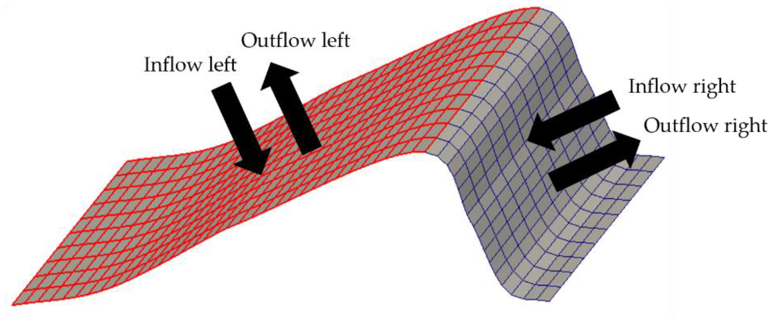
| Case | Inflow Left (m3/s) | Inflow Right (m3/s) | Inflow Sum (m3/s) | Outflow Left (m3/s) | Outflow Right (m3/s) | Outflow Sum (m3/s) | Total Flux 1 (m3/s/m2) |
|---|---|---|---|---|---|---|---|
| 1 | 2.9 × 10⁻⁴ | 3.8 × 10⁻⁵ | 3.3 × 10⁻⁴ | 2.1 × 10⁻⁴ | 1.2 × 10⁻⁴ | 3.3 × 10⁻⁴ | 2.7 × 10⁻³ |
| 2 | 1.4 × 10⁻⁴ | 6.3 × 10⁻⁶ | 1.4 × 10⁻⁴ | 3.7 × 10⁻⁵ | 1.3 × 10⁻⁴ | 1.6 × 10⁻⁴ | 5.1 × 10⁻³ |
| 3 | 6.6 × 10⁻⁴ | 5.3 × 10⁻⁵ | 7.2 × 10⁻⁴ | 4.9 × 10⁻⁴ | 2.4 × 10⁻⁴ | 7.3 × 10⁻⁴ | 3.0 × 10⁻³ |
| 4 | 4.0 × 10⁻⁴ | 6.1 × 10⁻⁵ | 4.6 × 10⁻⁴ | 3.3 × 10⁻⁴ | 1.6 × 10⁻⁴ | 4.9 × 10⁻⁴ | 2.2 × 10⁻³ |
| 5 | 4.2 × 10⁻⁴ | 6.0 × 10⁻⁵ | 4.8 × 10⁻⁴ | 1.7 × 10⁻⁴ | 2.9 × 10⁻⁴ | 4.6 × 10⁻⁴ | 3.9 × 10⁻³ |
| 6 | 1.2 × 10⁻⁴ | 2.0 × 10⁻⁵ | 1.4 × 10⁻⁴ | 9.6 × 10⁻⁵ | 4.8 × 10⁻⁵ | 1.4 × 10⁻⁴ | 2.9 × 10⁻⁴ |
| Case | Inflow Left (m3/s) | Inflow Right (m3/s) | Inflow Sum (m3/s) | Outflow Left (m3/s) | Outflow Right (m3/s) | Outflow Sum (m3/s) | Total Flux 1 (m3/s/m2) |
|---|---|---|---|---|---|---|---|
| 1 | 2.2 × 10⁻³ | 2.5 × 10⁻⁵ | 2.2 × 10⁻³ | 1.0 × 10⁻³ | 1.2 × 10⁻³ | 2.2 × 10⁻³ | 1.8 × 10⁻² |
| 2 | 5.6 × 10⁻⁴ | 2.9 × 10⁻⁵ | 5.9 × 10⁻⁴ | 1.6 × 10⁻⁴ | 3.7 × 10⁻⁴ | 5.2 × 10⁻⁴ | 1.8 × 10⁻² |
| 3 | 4.5 × 10⁻³ | 3.8 × 10⁻⁵ | 4.6 × 10⁻³ | 1.5 × 10⁻³ | 2.1 × 10⁻³ | 3.6 × 10⁻³ | 1.7 × 10⁻² |
| 4 | 3.5 × 10⁻³ | 0 | 3.5 × 10⁻³ | 2.0 × 10⁻³ | 1.9 × 10⁻³ | 3.9 × 10⁻³ | 1.7 × 10⁻² |
| 5 | 3.6 × 10⁻³ | 0 | 3.6 × 10⁻³ | 8.4 × 10⁻⁴ | 2.2 × 10⁻³ | 3.1 × 10⁻³ | 2.7 × 10⁻² |
| 6 | 9.3 × 10⁻⁴ | 1.4 × 10⁻⁵ | 9.4 × 10⁻⁴ | 4.6 × 10⁻⁴ | 5.2 × 10⁻⁴ | 9.8 × 10⁻⁴ | 1.9 × 10⁻³ |
© 2019 by the authors. Licensee MDPI, Basel, Switzerland. This article is an open access article distributed under the terms and conditions of the Creative Commons Attribution (CC BY) license (http://creativecommons.org/licenses/by/4.0/).
Share and Cite
Broecker, T.; Teuber, K.; Sobhi Gollo, V.; Nützmann, G.; Lewandowski, J.; Hinkelmann, R. Integral Flow Modelling Approach for Surface Water-Groundwater Interactions along a Rippled Streambed. Water 2019, 11, 1517. https://doi.org/10.3390/w11071517
Broecker T, Teuber K, Sobhi Gollo V, Nützmann G, Lewandowski J, Hinkelmann R. Integral Flow Modelling Approach for Surface Water-Groundwater Interactions along a Rippled Streambed. Water. 2019; 11(7):1517. https://doi.org/10.3390/w11071517
Chicago/Turabian StyleBroecker, Tabea, Katharina Teuber, Vahid Sobhi Gollo, Gunnar Nützmann, Jörg Lewandowski, and Reinhard Hinkelmann. 2019. "Integral Flow Modelling Approach for Surface Water-Groundwater Interactions along a Rippled Streambed" Water 11, no. 7: 1517. https://doi.org/10.3390/w11071517