Development of a Contaminant Distribution Model for Water Supply Systems


1
French South African Institute of Technology (F’SATI)/Department of Electrical Engineering, Tshwane University of Technology, Pretoria 0001, South Africa
2
École Supérieure d’Ingénieurs en Électrotechnique et Électronique, Cité Descartes, 2 Boulevard Blaise Pascal, Noisy-le-Grand, 93160 Paris, France
3
Institute of NanoEngineering Research (INER)/Department of Chemical, Metallurgy and Material Engineering, Tshwane University of Technology, Pretoria 0001, South Africa
*
Author to whom correspondence should be addressed.
Water 2019, 11(7), 1510; https://doi.org/10.3390/w11071510
Submission received: 21 June 2019
/
Revised: 12 July 2019
/
Accepted: 17 July 2019
/
Published: 21 July 2019
(This article belongs to the Section Water Quality and Contamination)
Abstract
:Water contamination can result in serious health complications and gross socioeconomic implications. Therefore, identifying the source of contamination is of great concern to researchers and water operators, particularly, to avert the unfavorable consequences that can ensue from consuming contaminated water. As part of the effort to address this challenge, this present study proposes a novel contaminant distribution model for water supply systems. The concept of superimposing the contaminant over the hydraulic analysis was used to develop the proposed model. Four water sample networks were used to test the performance of the proposed model. The results obtained displayed the contaminant distributions across the water network at a limited computational time. Apart from being the first in this domain, the significant reduction of computational time achieved by the proposed model is a major contribution to the field.
1. Introduction
The provision of potable water is essential to human health and the well-being of a society. This also conforms with one of the set objectives (target 6a) of the United Nation’s sustainable Development Goals (SDGs) by 2030 [1]. Despite reports that access to water have improved, a depleted delivery of potable water is an utmost concern that affects several continents. Interestingly, the goal of a utility operator is to supply water in adequate quantity and quality when desired. Usually, water is transported through water distribution networks (WDNs) from a treatment plant to consumers’ taps. A WDN is a complex infrastructure, which comprises of: pipes, nodes, and reservoirs where human interference is possible. Hence, it is exposed to both accidental and intentional attacks, which can have severe consequences on the public health, besides socioeconomic implications [2,3].
Mostly, the quality of water is examined at a treatment plant, but it can technically be contaminated during transportation, through: pipe leakages, nodes and cross-connections [4]. The negative consequences of consuming contaminated water can be severe, as reported in the literature [5]. For instance, Kenzie et al. [6] and Corso et al. [7] discussed the significant impact of a transported infection through a water supply system in Milwaukee, (USA) that engendered 403,000 users, some were subsequently hospitalised with an estimated bill of about USD 96.2 million. Cooper et al. [8] reported the consequences of an accidental pollution of a chemical in a WDN in Virgina, where over 300,000 users were affected. Several studies [6,7,8] have also established that attacks on the WDNs are real, and can happen again. The socioeconomic implications that can arise from water network attacks have allowed researches on water security, a notable attention and posited it at the forefront of research in this area.
Consequently, two notable preventive measures are recognised to curtail the attacks on the WDNs. These are: (1) enhancement of the physical infrastructure of the system, and (2) an instalment of water quality monitoring sensors across the water networks. An intensive monitoring of the network nodes will increase the level of safety. Unfortunately, it is impracticable to install sensors at every node in the network due to the high cost of procuring water quality monitoring sensors under limited budget constraints. In order to overcome these constraints, numerous efforts have been proposed to address the concern [9,10,11,12,13,14,15,16,17]. Even though an installed water quality sensor detects a contaminant event, it is imperative to identify the source of the contamination for immediate action to be taken, so as to minimise the adverse effect from contaminated water on the public health.
As such, research efforts on the Contamination Source Identification (CSI) in a water distribution network has significantly gained recognition. Modelling the transport and fate of contaminant in a WDN, demands knowledge about the characteristics of the contaminant, which are hardly known. Furthermore, it is rarely possible to identify the name of the contaminant and its type (chemical or biological); these add to the complexity encountered in developing a precise water quality model. Researchers and stakeholders have proposed various methodologies to address this challenge [13,18,19,20,21,22,23]. Adedoja et al. [5] presented a comprehensive review on how to establish a source of contamination in a water distribution network. Since hydraulic model exists and has been solved by some researchers [24,25,26,27], incorporating contaminant into it is a promising approach. Superimposing the contaminant into the hydraulic model has no effect on the flow direction. Based on this background, this study develops, a contaminant distribution model, by superimposing contaminants into the hydraulic analysis in order to quantify the contaminant distribution across the water networks. This is part of an effort to bridge the identified research shortcomings and contribute to knowledge in this domain. The rest of this paper is organised as follows: Section 2 outlines a brief background and related works. In Section 3, the description of the hydraulic model and the proposed mathematical formulation is presented. Implementation of the developed model on water networks is detailed in Section 4. Results and discussions are contained in Section 5, while conclusions and future research studies are presented in Section 6.
2. Background and Related Works
The CSI problem is characterised by responding to three (3) vital concerns: locating the source of contamination, the time of injection, and its magnitude. A derivation of the information from the data collected from water quality monitoring stations, is a complex task that must be resolved for prevention purposes, which include: public warning announcements, valves closure, pipes flushing, etc. Over the years, researchers have proposed different approaches; the use of simulation-optimisation approach [18], particle backtracking [28], machine learning [29], data mining [30], among others. CSI problem is commonly treated as an inverse problem by attempting to locate the source of contamination from the data collected from the water quality monitoring stations. Van Bloemen et al. [31] proposed a quadratic programming (QP) technique to tackle this problem. The authors’ model exhibited a probable capability to address the challenge. However, excessive computational stress was identified as a shortcoming of their approach. Thereafter, Lair et al. [32] suggested a dynamic optimisation method, based on a sub-domain to curtail this computational stress. They reported that the model can merely handle the computational stress, but excludes key information during the selection of sub-domains, which was a setback of the approach.
Preis and Ostfeld [33] presented a coupled model tree-linear programming technique with the use of the commonly adopted EPANET tool developed by Rossman [34]. Preis and Ostfeld [35] proposed a combination of a Generic algorithm (GA) with the EPANET to resolve the CIS problem. EPANET was employed for the hydraulic simulation, while GA was used to moderate the injection attribute. The method minimises the difference between the measured and the evaluated data. The use of this method requires an excessive computation that demands the use of parallel computing. In addition, the study by Liu et al. [22,23] discussed an adaptive dynamic optimisation (ADOPT) method. This method has a real-time response with contamination occurrences. The authors utilised an evolutionary algorithm (EA) to overcome the early convergence that can lead to imprecise output. This process helps to preserve a group of possible output that can lead to diverse non-unique solutions. The EA enhances the results once a new observation is absorbed, which decreases the magnitude of the non-uniqueness. It was tested by using two water networks to demonstrate the feasibility of the proposed method. The consideration of a single source of injection and non-reactive contaminants are some of the advantages of this method; however, for a large water network, such assumptions may not be feasible. The model may therefore, suffer from over-generalization. Recently, Xu et al. [19] used a cultural algorithm to address a similar concern. They demonstrated the viability of the method by using three water supply networks. The results obtained exhibited positive capability of the technique, even though extreme computation was a major setback. Other shortcomings connected to the CSI problems are: complex network nodes, and stochaistic demand of water, which can lead to some problems of uncertainties. Yan et al. [36] proposed a hybrid encoding method to improve the convergence criteria.
Probabilistic and Bayesian techniques have also been used to address CSI problem. Dawsey et al. [37] proposed an inclusion of sensor data with a possibility to evaluate the source of occurrence from different areas, while Tao et al. [38] formulated a probabilistic approach. Nuepauer et al. [39] presented a backward modelling scheme with the use of a Probability Density Function (PDF) to locate the source and release time of contamination. The collected information from the monitoring sensor were used to generate the PDF. The results obtained expressed the effectiveness of the backward model to handle a steady flow conditions with a single source of the contamination. Wang and Zhou [40] applied a Bayesian sequential technique to handle the CSI problem. Baradouzi et al. [41] discussed a Probabilistic Support Vector Machines (PSVMs) technique to identify the source of contamination; they used some tools to train the PSVMs. The results obtained exhibit the feasibility of the approach to identify an upstream region viable for likely location. The water distribution system of Arak, Iran was employed to validate the proposed method.
Other notable works have been presented by Di Nardo et al. [42], model-based by Zechman and Ranjithan [20], artificial neutral networks, (ANN) by Kim et al. [43] and hybrid methods [44,45] to resolve the CSI problem. Propato [13] discussed an entropic-based method. In the study, a linear algebraic technique was first employed to minimise the selection of probable sources. Thereafter, a minimum entropy method was applied to evaluate the likely source, which led to the potential sources that are sensible to the monitoring stations. An evolutionary scheme and population-based global search method was presented by Zechman and Ranjithan [20]. The technique was devised by applying a tree-based encoding model, which generates the decision vectors and a set of connected genetic operators that led to an effective search. Liu et al. [45] combined a statistical method and a heuristic search model to present the contamination incident. The statistical method pointed the possible locations and the heuristic search method amplified the contamination source attributes. The feasibility of the method was examined by using two water networks. The results obtained showed a quick adaptive discovery of contaminant attributes. However, the method cannot be expanded to handle multiple sources occurrence. Liu et al. [44] proposed a hybrid method to characterise the sources by giving a sensor measurements in real time. The method integrates a logistic regression (LR) and local improvement model to speed-up the convergence processes. In order to ascertain the capability of the method, two water networks were examined. The first is a sample small network of about 117 pipes, while the details of the second network was adapted from [46]. The results obtained, expressed the fast convergence of the hybrid method when compared to the single method. Despite the significant effort recorded on the aforementioned problem, excessive computation remained unsolved. To this end, the present study formulates a contaminant distribution model when given the source of contamination, with an assumption that hydraulic solution is solved.
3. Proposed Model Formulation
Since hydraulic model exists and have been solved by some researchers [24,26], this study proposes to superimpose the contaminant into the hydraulic analysis. This study formulates a contaminant distribution model by giving a source of contaminations and, on an assumption that the hydraulic model is resolved and the network flow analysis is known.
3.1. Hydraulic Model
By applying graph the theory, a water distribution network can be presented as a connected graph with a set of edges and a set of nodes [24]. The former consists of pipes, pumps and valves. The two basic principles that describe the hydraulic equations in a water distribution network are: the principle of mass continuity in the node and, an energy conservation around the loop. A typical water network consist of number of pipes, number of junction nodes (nodes with unknown heads), and number of fixed-head nodes (nodes with known heads), the total number of nodes in the network can be expressed as: = + . The mass continuity equation is similar to the Kirchoff’s law in electrical network and, it is applicable to the nodes with known demand. It states that the algebraic summation of the flows at the node is zero. Thus, it is expressed as:
where is the vector of the pipe flow rates; is the vector of the fixed demand at the nodes with unknown heads and is the node-pipe incidence matrix of dimension connecting to the nodes with unknown heads [47]. The energy conservation law is related to the Kirchoff’s voltage law in electrical network. It deals with head losses around the loops and, can be presented in term of its topological matrix as follows:
where is the head loss vector across the pipes; is the head loss across the loops; represented the loop-pipe incidence matrix; and m is the number of loops. The element in Equation (2) are derived from:
In addition, the energy conservation is expressed, thus:
where denotes the vector of the unknown heads of dimension ) and represents the vector of the unknown heads of dimension ). is the node-pipe incidence matrix of dimension associating to the nodes with unknown heads [47]. Both and are obtained from the actual topological incidence matrix, A as:
The element A is derived from
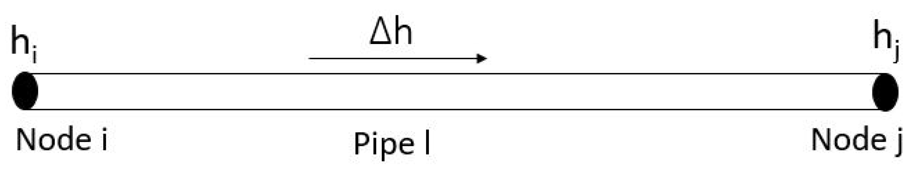
Similarly, the head loss equations are essential for the solution of the piping networks. It describes the pressure drop across a given pipe of flow in a particular pipe. An illustration of this is described by the element shown in Figure 1, with two end nodes i and j. The head loss due to the friction of the flow of water with the pipe wall is commonly expressed as:
where and are the heads at end node of the pipe and denotes the vector of the pipe resistance factor. Consideration of minor loss due to the valves and other pipe connections is generally expressed in the form:
Subsequent, consideration of energy balance equation and the inclusion of the minor loss leads to;
A matrix E can be defined as:
By substituting Equations (12) into (11), the energy balance equation is expressed as
Equations (1) and (13) are both steady-state hydraulic equations. These can be solved in order to estimate the pipe flow and the heads at the junction node. The system of equations expressed by Equation (14) are partly linear and partly non-linear [24].
Equation (14) can also be expressed as:
The system of equations expressed in the Equation (14) maybe solved by an iterative method. The matrix E is a diagonal matrix, whose elements are formed from the head loss (including the minor loss due to valves) relation as:
where is a ) vector of the minor loss factor due to valves or any other connections attached to the pipe; and is an exponent whose value depends on the head loss model employed (1.85 for Hazen–Willam and 2 for both Darcy–Weisbach or Chezy–Manning head loss model) [48]. The variable r depends on the head loss model employed. In the circumstance where the Darcy–Weisbach or the Hazen–William’s model is used, the hydraulic resistance for the pipe is described as:
for Darcy-Weisbach model, and
for Hazen-William model. In Equations (17) and (18), is the length of the pipe; g is the acceleration due to gravity; denotes the diameter of the pipe; is a dimensionless constant, which represents the fictional factor for the pipe; and is the Hazen–William friction coefficient for the pipe. The pipe friction factor f, in Equation (17) is a function of the equivalent sand roughness of pipes as well as the Reynold number , and this can be calculated by using the expression reported by Shockling et al. 2006 [49]. In this study, the Hazen–William head loss model will be adopted.
3.2. Formulation of the Proposed Contaminant Distribution Model
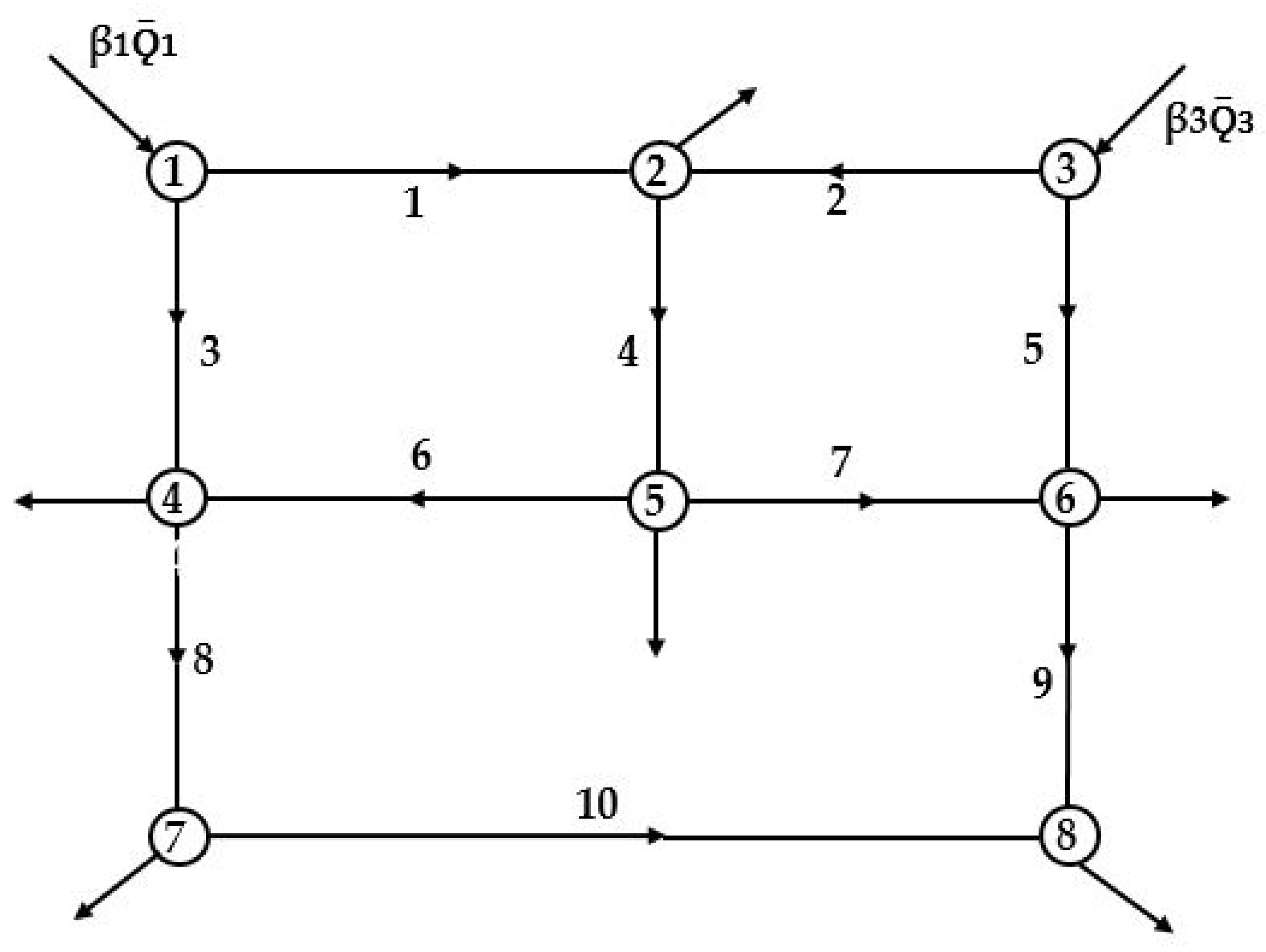
The formulation of this model assumes that the hydraulic solution has been resolved and the source of contaminations are known. Thus, the proposed contaminant distribution model is explicitly presented by using Figure 2.
The simple network depicted in Figure 2 consists of Eight (8) nodes, and Ten (10) branches. In this case, nodes 1 and 3 are assumed to be the sources of contamination with variables; and while, the external sources are represented by; and respectively. The concentrations at nodes: 1 to 8 are independent of the inflow branches into a particular node. By assigning a variable , to the concentration at node k, the following relationships are formulated in Equations (19)–(26) as:
Considering the out of the node concentrations. If concentrations in branches are represented by , then Equations (26)–(33) are formulated as:
Therefore, the concentration of contamination at node k is independent of the outflow branches from the respective nodes; this is expressed in Equation (34)
where in Equation (34) is expressed in Equation (35) and is the transpose of the incident matrices, is the concentration at node k and is the concentration in branches.
Similarly, the inflow , into the nodes is formulated in Equations (36)–(43) as:
The matrices formulation of Equations (36)–(43) is expressed in Equation (44) as:
Equation (44) is generally expressed in Equation (45) as:
where in Equation (45) is the transpose of the inflow incident matrices and expressed in Equation (46), is the flow and , is the flow from the external sources.
The integration of the concentration at node, and flow at node, q can be expressed in term of flow, Q. Thus, the concentration in branches (i.e., pipes) , are formulated and expressed in Equations (47)–(54) as:
Equations (47)–(54) are represented in matrices form in Equation (55)
The general formulation of Equation (55) is expressed in Equation (56) as:
The concentration in branches , is related to the concentration at node and is expressed in Equation (57) as:
Equation (57) is generally expressed in Equation (58) as:
If Equation (58) is substituted into Equation (56), then, Equation (59) is expressed as:
By resolving Equation (60), may be derived. Therefore, the distribution of contaminants across the pipes and at the nodes can be quantified.
4. Application of the Developed Model on WDNs
The validation of the developed contaminant distribution model was implemented on four water distribution networks, which were adapted from literature [47,50,51]. All computations and hydraulic analysis were performed in MATLAB software environment.
4.1. Model Programming Procedures
This procedure assumes that the hydraulic network analysis has been resolved. In this study, Newton–Raphson’s Content Model solution is employed [24]. The required input from the solved network analysis are; sending nodes, receiving nodes and the flow . Thus, the program procedures are as follow:
- Get the network analysis solution
- Prepare the Structure
- Get the pipe flows
- Get supplies and demands
- Get injections at the supply nodes
- Get contamination at supply nodes
- Compute the sum input flows to the nodes
- Build matrices for equation as function of gamma, .
- Compute contamination at the nodes
- Get contamination in the pipes, .
4.2. Illustrative Example 1
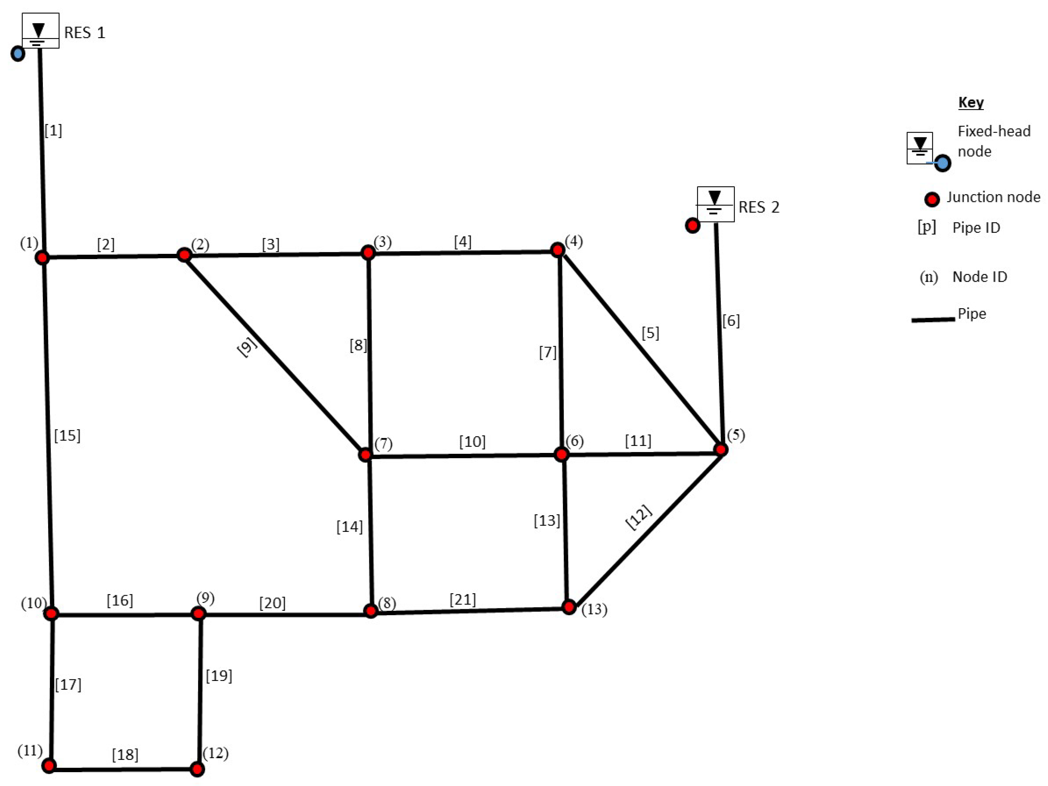
Figure 3 is a water distribution network adapted from the work of Ozger [50], to demonstrate the validity of the developed contaminant distribution model. The network has two (2) reservoirs with twenty-one (21) Pipes, and (13) thirteen Nodes. In this example, it is assumed that 3% and 2% of the flow are injected at reservoir 1 and 2 as contaminants, respectively. The available network characteristics are presented in Table 1.
4.3. Illustrative Example 2
4.4. Illustrative Example 3
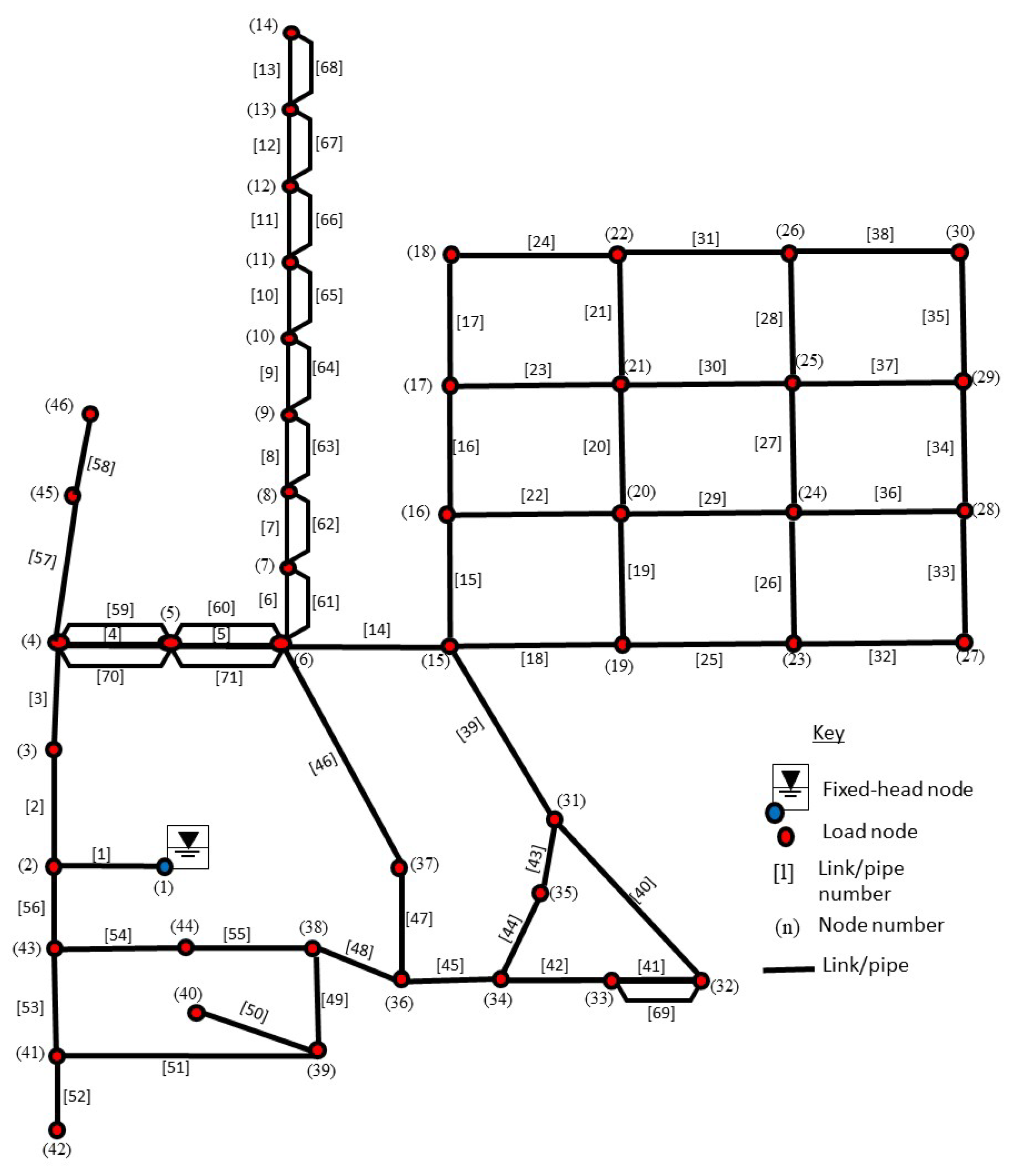
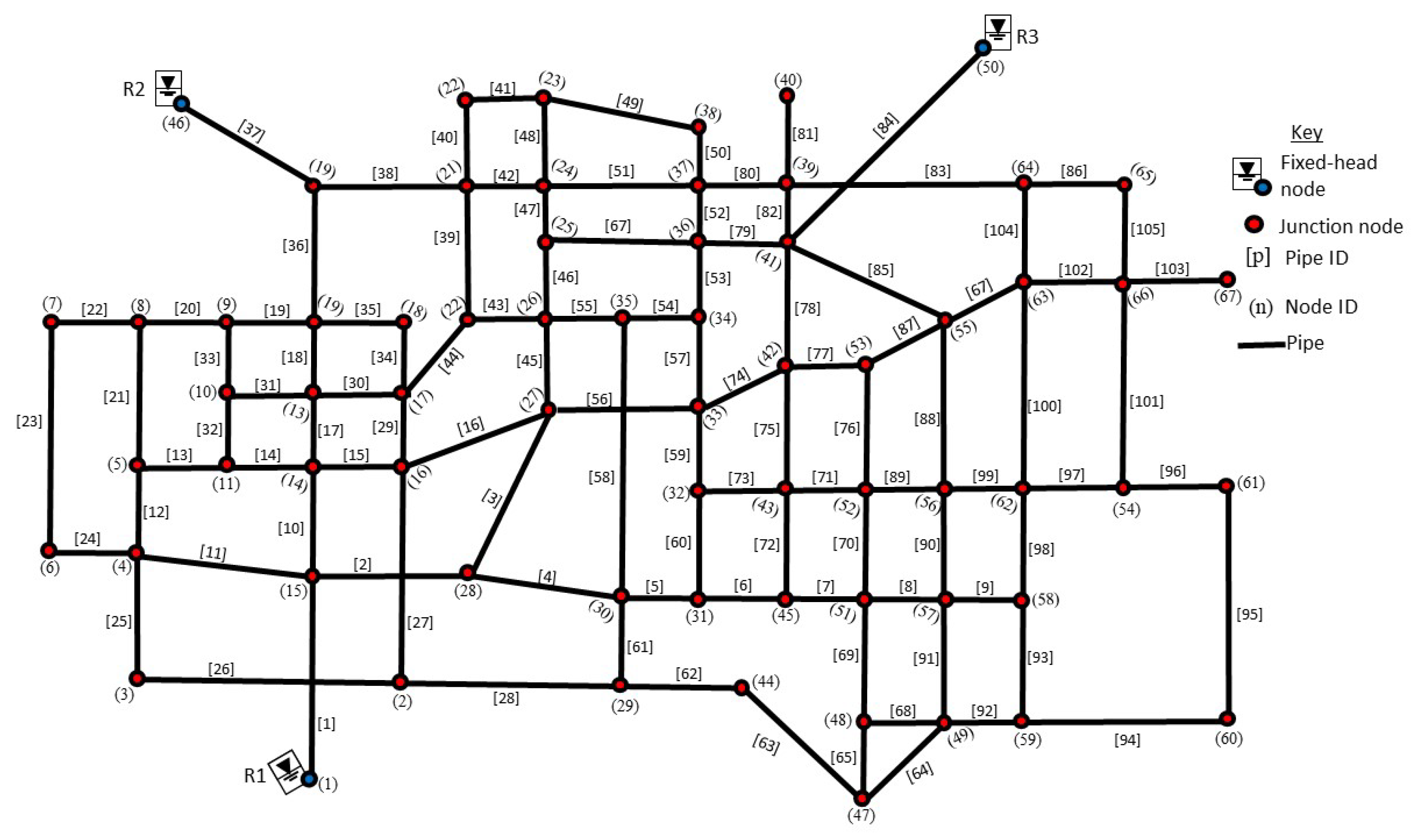
In this example, one hundred and five (105) pipes network depicted in Figure 4, was considered. The network consists of 105 pipes, three fixed-head nodes (sources), and 64 nodes, after redundant nodes (these are nodes where two or more pipes meet with zero demand) were removed. The network characteristic data defining the network is available in the report of Adedeji [47].
4.5. Illustrative Example 4
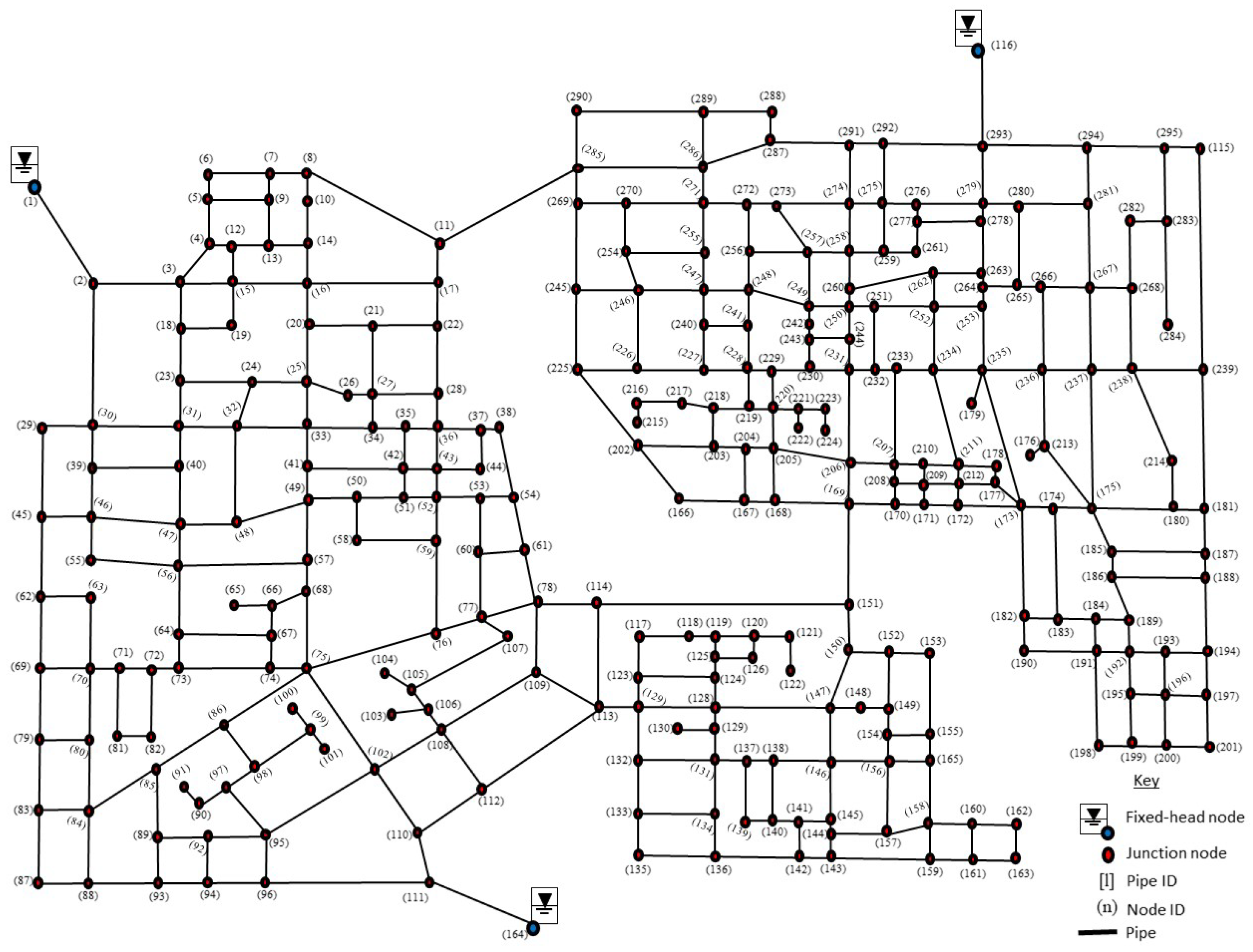
This example examined the four hundred and forty two pipes as represented in Figure 5. The network contains 442 pipes, three reservoirs, and 295 nodes after the redundant (these are nodes where two or more pipes meet with zero demand) nodes have been removed. The data defining the network is available in the report by Adedeji [47].
5. Results and Discussions
This section presents the results and discussions of the four (4) sample networks examined for the validation of the performance of the developed model. Table 2 and Table 3 present the numerical results for illustrative Example 1.
5.1. Results and Discussions for Illustrative Example 1
The results of the pipe flow and the contaminant in the pipes are presented in Table 2. This Table shows that Pipe 7 has contaminant concentration of 0.029; it is as a result of the combination of the contaminants from Nodes 1 and 2 at Node 4. At Pipes 5, 6, 11, 12, and 21, the contaminants are from the same source, Node 2, while the other pipes have the same contaminant concentration (0.030); this implies that the contaminant is from Node 1. Based on these results, pipes with the same node as origin, have the same contaminant concentration, for example, Pipes, 5, 6, 11, 12, and 21. However, where different contaminant mix at a node, the contaminant concentration that will leave the node will be less than the maximum contaminant concentration that enters the node. A typical example of this scenario is at Pipe 7. On the other hand, when the quantity of contaminants from different pipes meeting at a node are the same, the contaminant concentration leaving the node will be the average of the contaminant concentration that entered into the node. Thus, this shows that the proposed model results are realistic.
The nodal flow and contaminant distribution at nodes for illustrative Example 1, is shown in Table 3. The results in this Table shows that Nodes 4 (0.029), 6 (0.024), and 8 (0.024) have different contaminant concentrations. These concentrations are different from the injected contaminant concentrations, which are 0.030 and 0.020 from Nodes 1 and 2, respectively. This difference in the contaminants’ concentration is due to different contaminants mixing at a node. On the other hand, when different sources with the contaminant concentrations mix at a node, the node’s contaminant concentration is the same as its source concentration.
5.2. Results and Discussions for Illustrative Example 2
Table 4 and Table 5 present the numerical results of contaminant contribution for the pipes and nodes for illustrative Example 2. The Illustrative Example 2, as shown in Figure 4, has only one source of supply, and 5% of the flow is assumed as contaminant. Since, there is no contaminant mix, it is reasonable for the 0.050 contaminants injected at the source to flow through the entire network, which also verified the feasibility of the proposed model. The results of the pipes and nodes flow rate are also presented. A sub-network with area nodes: 15, 18, 30 and 27 revealed that the quantity of contaminants decreases from node 15 towards node 18. Similar attribute was observed from node 15 towards node 27. Perhaps, if there is a need for water piping extension, it will be appropriate to tap from the extreme nodes, irrespective of the node position. This is because, nodes at the extreme nodes have lower quantity of contaminants. It was generally observed that the farther the node from the source of supply, the lower the quantity of contaminant at the nodes junction.
5.3. Results and Discussions for Illustrative Example 3
Table 6 and Table 7 present the numerical results of the contaminant contribution across the pipes and the nodes for illustrative Example 3. In this example, it was assumed that Nodes 1, 46, and 50 are sources of contamination with 0.04, 0.05 and 0.03 contaminants, respectively. This example has redundant nodes (these are nodes where two or more pipes meet with zero demand), which were excluded in the simulations. The node numerical results obtained (Table 7) revealed that most of the nodes have different contaminant values from injected contaminants at the three (3) sources (Nodes; 1, 46, and 50) of contamination. This is due to the fact that, different contaminants mix at different nodes of the networks. It was observed that the contaminant (0.04) at source (Node 1) flows through Node 1 to 6; 10–11; 14–16; 27 and 28, respectively. These nodes have direct connections to the source (Node 1) without mixing with the two sources of contaminant, as can be seen in the schematic diagram of the network in Figure 5. Similarly, the contaminant from source (Node 46) flows through Nodes; 46, 19, 21, and 22, respectively. These nodes are also directly connected to the source (Node 46) without any interconnected nodes from other sources of contamination. This same attribute was observed from source (Node 50) where Nodes; 41, 36, 34, 35, 33, 41, 53 and 55 have the same contaminant values that was injected at source (Node 50). On the other hand, contaminant at the remaining nodes differ from the injected values (ranges between the lowest to highest values. i.e., 0.030–0.050). Based on the results obtained, the values of contaminants from Nodes 7–13 range between the contaminant values from Nodes 1 and 46 (i.e., 0.040–0.050). The results showed that these nodes have contaminant mixtures from the stated nodes (i.e., Nodes 1 and 46). Similar attribute was observed at Nodes; 17, 18, 20, 23, and 24. The results of the remaining nodes indicated a mixture of contaminants from source Nodes 1 and 50. These can be seen from the numerical results for Nodes 47 to 67. Moreover, circumstances where three contaminants mix at the nodes are possible within the network. This further established the practicability of the proposed model as observed from the results.
The numerical results of pipe and contaminant flow for the Illustrative Example 3 is presented in Table 6. Similar to the node results, it was observed that pipes that are directly connected to the sources of contaminants have same flow as their sources. For instances, Pipes 1–4, 10–17, 23–29 are directly connected to source (Node 1). Similar scenarios are observed in Pipes; 36–42, which are connected to source (Node 46). Likewise, the Pipes connected to source (Node 50) are 52–55, 57–58, 72–77, 80, 82–85, and 105, respectively. The rest of the pipes are connected to the nodes where two or more contaminants mix as noted from the results obtained.
5.4. Results and Discussions for Illustrative Example 4
After the removal of redundant nodes (these are nodes where two or more pipes meet with zero demand), the illustrative Example 4 network consists, 442 pipes, three reservoirs, and 295 nodes as depicted in Figure 6. This network sample is bigger than Example 3 network, and they both have three sources of contaminations. In this case, nodes 1, 116, and 164 are assumed to be contamination sources with; 0.02, 0.01, and 0.03, respectively. The contaminant distributions across this network displayed the same attributes as the results of the Illustrative Example 3. The proposed method shows capability to handle medium networks within a short time. The results of Illustrative Example 4 is not presented due to its volume.
Table 8 shows the number of iterations taken in order to obtain the result for the various WDNs considered. As expected, the number of iterations increases as the size of the WDN increases.
Table 9 depicts the execution time for both hydraulic analysis and the proposed model for the various WDNs considered in this study. It was generally observed that the bigger the network, the higher the execution time.
6. Conclusions and Future Studies
Over the years, identification of contamination sources has received a significant attention among researchers and, has been a concern due to the negative effect that can emanate from the use of contaminated water. As part of an effort to fill this research gap, this study proposed a contaminant distribution model by superimposing the contaminant over the network analysis. To the best of the authors’ knowledge, there is no record of this approach in the literature. The viability of the proposed model was tested with four water networks, and the model’s performance was satisfactory. The results obtained described the practicability of the contaminant distribution across pipes and the nodes of the water networks. In addition, the results verified the practicability of the proposed model at a limited computational time. The source of contamination could be derived with this distribution model if, a set of measurement data is given. Thus, this will allow water supply companies to know the source of contamination upon which appropriate preventive measures such as; public awareness, closure of valves, etc. would be provided in order to minimise the extent of contamination on the society. In addition, comparison of this model with similar methodologies is important in order to ascertain its strength and weakness which, would be examined in future studies. Furthermore, procurement and maintenance cost of water quality monitoring sensor is also a challenge that must be addressed. Future research would focus on the issue of contamination source identification and optimal sensor placement in a water distribution network. The proposed model and its solution will be embedded within a method that allows the detection of the source of contamination. Although, this model was applied on a small and medium WDNs due to data availability, application of the proposed model on large networks would also be investigated in the future. These are topical areas of research interest that would be examined in subsequent studies. Finally, in order to increase the dynamics and robustness of the proposed model, it is expected that future research will explore the effects of external factors, such as temperature, on the contaminant distribution model.
Author Contributions
The work is part of the Doctorate degree of O.S.A. which was discussed with his supervisors. O.S.A. formulated the problem and drafted the manuscript. Y.H. assisted with quality improvement in the mathematical formulations and programming. The manuscript was scrutinized by Y.H. and R.S. while, B.K. also gave some suggestions.
Acknowledgments
This research work was supported by the French South African Institute of Technology (F’SATI), Tshwane University of Technology, Pretoria, South Africa.
Conflicts of Interest
The authors declare no conflict of interest.
References
- Sdgreport. The Sustainable Development Goals 2015. 2015. Available online: www.undp.org/content/undp/en/home/sustainable-development-goals/goal-6-clean-water-and-sanitation.html (accessed on 18 May 2019).
- Clark, R.M.; Grayman, W.M.; Males, R.M. Contaminant propagation in distribution systems. J. Environ. Eng. 1988, 114, 929–943. [Google Scholar] [CrossRef]
- Clark, R.M.; Deininger, R.A. Protecting the nation’s critical infrastructure: The vulnerability of US water supply systems. J. Contingencies Crisis Manag. 2000, 8, 73–80. [Google Scholar] [CrossRef]
- Kirmeyer, G.J.; Martel, K. Pathogen Intrusion into the Distribution System; American Water Works Association: Denver, CO, USA, 2001. [Google Scholar]
- Adedoja, O.S.; Hamam, Y.; Khalaf, B.; Sadiku, R. Towards Development of an Optimization Model to Identify Contamination Source in a Water Distribution Network. Water 2018, 10, 579. [Google Scholar] [CrossRef]
- Mac Kenzie, W.R.; Hoxie, N.J.; Proctor, M.E.; Gradus, M.S.; Blair, K.A.; Peterson, D.E.; Kazmierczak, J.J.; Addiss, D.G.; Fox, K.R.; Rose, J.B.; et al. A massive outbreak in Milwaukee of Cryptosporidium infection transmitted through the public water supply. N. Engl. J. Med. 1994, 331, 161–167. [Google Scholar] [CrossRef] [PubMed]
- Corso, P.S.; Kramer, M.H.; Blair, K.A.; Addiss, D.G.; Davis, J.P.; Haddix, A.C. Costs of illness in the 1993 waterborne Cryptosporidium outbreak, Milwaukee, Wisconsin. Emerg. Infect. Dis. 2003, 9, 426. [Google Scholar] [CrossRef] [PubMed]
- Cooper, W.J. Responding to crisis: The West Virginia chemical spill. Environ. Sci. Technol. 2014, 48, 3095. [Google Scholar] [CrossRef] [PubMed]
- Berry, J.W.; Fleischer, L.; Hart, W.E.; Phillips, C.A.; Watson, J.P. Sensor placement in municipal water networks. J. Water Resour. Plan. Manag. 2005, 131, 237–243. [Google Scholar] [CrossRef]
- Berry, J.; Carr, R.D.; Hart, W.E.; Leung, V.J.; Phillips, C.A.; Watson, J.P. Designing contamination warning systems for municipal water networks using imperfect sensors. J. Water Resour. Plan. Manag. 2009, 135, 253–263. [Google Scholar] [CrossRef]
- Ostfeld, A.; Salomons, E. Optimal layout of early warning detection stations for water distribution systems security. J. Water Resour. Plan. Manag. 2004, 130, 377–385. [Google Scholar] [CrossRef]
- Ostfeld, A.; Salomons, E. Optimal early warning monitoring system layout for water networks security: Inclusion of sensors sensitivities and response delays. Civ. Eng. Environ. Syst. 2005, 22, 151–169. [Google Scholar] [CrossRef]
- Propato, M. Contamination warning in water networks: General mixed-integer linear models for sensor location design. J. Water Resour. Plan. Manag. 2006, 132, 225–233. [Google Scholar] [CrossRef]
- Kansal, M.; Dorji, T.; Chandniha, S.K. Design scheme for water quality monitoring in a distribution network. Int. J. Environ. Dev. 2012, 9, 69–81. [Google Scholar]
- Afshar, A.; Khombi, S.M. Multiobjective optimization of sensor placement in water distribution networks; dual use benefit approach. Int. J. Optim. Civil. Eng. 2015, 5, 315–331. [Google Scholar]
- Cozzolino, L.; Mucherino, C.; Pianese, D.; Pirozzi, F. Positioning, within water distribution networks, of monitoring stations aiming at an early detection of intentional contamination. Civ. Eng. Environ. Syst. 2006, 23, 161–174. [Google Scholar] [CrossRef]
- Ostfeld, A.; Uber, J.G.; Salomons, E.; Berry, J.W.; Hart, W.E.; Phillips, C.A.; Watson, J.P.; Dorini, G.; Jonkergouw, P.; Kapelan, Z.; et al. The battle of the water sensor networks (BWSN): A design challenge for engineers and algorithms. J. Water Resour. Plan. Manag. 2008, 134, 556–568. [Google Scholar] [CrossRef]
- Laird, C.D.; Biegler, L.T.; van Bloemen Waanders, B.G.; Bartlett, R.A. Contamination source determination for water networks. J. Water Resour. Plan. Manag. 2005, 131, 125–134. [Google Scholar] [CrossRef]
- Yan, X.; Gong, W.; Wu, Q. Contaminant source identification of water distribution networks using cultural algorithm. Concurr. Comput. Pract. Exp. 2017, 29, e4230. [Google Scholar] [CrossRef]
- Zechman, E.M.; Ranjithan, S.R. Evolutionary computation-based methods for characterizing contaminant sources in a water distribution system. J. Water Resour. Plan. Manag. 2009, 135, 334–343. [Google Scholar] [CrossRef]
- De Sanctis, A.; Boccelli, D.; Shang, F.; Uber, J. Probabilistic approach to characterize contamination sources with imperfect sensors. In Proceedings of the World Environmental and Water Resources Congress 2008, Ahupua’A, HI, USA, 13–16 May 2008; pp. 1–10. [Google Scholar]
- Liu, L.; Ranjithan, S.R.; Mahinthakumar, G. Contamination source identification in water distribution systems using an adaptive dynamic optimization procedure. J. Water Resour. Plan. Manag. 2010, 137, 183–192. [Google Scholar] [CrossRef]
- Liu, L.; Zechman, E.M.; Brill, E.D., Jr.; Mahinthakumar, G.; Ranjithan, S.; Uber, J. Adaptive contamination source identification in water distribution systems using an evolutionary algorithm-based dynamic optimization procedure. In Proceedings of the Eighth Annual Water Distribution Systems Analysis Symposium, Cincinnati, OH, USA, 27–30 August 2006; pp. 1–9. [Google Scholar]
- Adedeji, K.B.; Hamam, Y.; Abe, B.T.; Abu-Mahfouz, A.M. Leakage Detection and Estimation Algorithm for Loss Reduction in Water Piping Networks. Water 2017, 9, 773. [Google Scholar] [CrossRef]
- Hamam, Y.; Brameller, A. Hybrid method for the solution of piping networks. In Proceedings of the Institution of Electrical Engineers; IET: London, UK, 1971; Volume 118, pp. 1607–1612. [Google Scholar]
- Hamam, Y.; Hindi, K. Optimised on-line leakage minimisation in water piping networks using neural nets. In Proceedings of the IFIP Working Conference, Dagschul, Germany, 28 September–1 October 1992; Volume 28, pp. 57–64. [Google Scholar]
- Todini, E. A unifying view on the different looped pipe network analysis algorithms. In Computing and Control for the Water Industry; Research Studies Press Ltd.: Baldock, UK, 1999; pp. 63–80. [Google Scholar]
- De Sanctis, A.E.; Shang, F.; Uber, J.G. Real-time identification of possible contamination sources using network backtracking methods. J. Water Resour. Plan. Manag. 2009, 136, 444–453. [Google Scholar] [CrossRef]
- Wang, H.; Harrison, K.W. Improving efficiency of the Bayesian approach to water distribution contaminant source characterization with support vector regression. J. Water Resour. Plan. Manag. 2012, 140, 3–11. [Google Scholar] [CrossRef]
- Huang, J.J.; McBean, E.A.; James, W. Multi-objective optimization for monitoring sensor placement in water distribution systems. In Proceedings of the Eighth Annual Water Distribution Systems Analysis Symposium, Cincinnati, OH, USA, 27–30 August 2006; pp. 1–14. [Google Scholar]
- Van Bloemen Waanders, B.G.; Bartlett, R.A.; Biegler, L.T.; Laird, C.D. Nonlinear programming strategies for source detection of municipal water networks. In Proceedings of the World Water & Environmental Resources Congress 2003, Philadelphia, PA, USA, 23–26 June 2003; pp. 1–10. [Google Scholar]
- Laird, C.D.; Biegler, L.T.; van Bloemen Waanders, B.G. Real-time, large-scale optimization of water network systems using a subdomain approach. In Real-Time PDE-Constrained Optimization; SIAM: Philadelphia, PA, USA, 2007; pp. 289–306. [Google Scholar]
- Preis, A.; Ostfeld, A. A contamination source identification model for water distribution system security. Eng. Optim. 2007, 39, 941–947. [Google Scholar] [CrossRef]
- Rossman, L.A. EPANET 2: Users Manual; National Risk Management Research Laboratory, U.S. Environmental Protection Agency: Cincinnati, OH, USA, 2000.
- Preis, A.; Ostfeld, A. Multiobjective sensor design for water distribution systems security. In Proceedings of the Eighth Annual Water Distribution Systems Analysis Symposium, Cincinnati, OH, USA, 27–30 August 2006; pp. 1–17. [Google Scholar]
- Yan, X.; Zhao, J.; Hu, C.; Wu, Q. Contaminant source identification in water distribution network based on hybrid encoding. J. Comput. Methods Sci. Eng. 2016, 16, 379–390. [Google Scholar] [CrossRef]
- Dawsey, W.J.; Minsker, B.S.; VanBlaricum, V.L. Bayesian belief networks to integrate monitoring evidence of water distribution system contamination. J. Water Resour. Plan. Manag. 2006, 132, 234–241. [Google Scholar] [CrossRef]
- Tao, T.; Huang, H.D.; Xin, K.L.; Liu, S.M. Identification of contamination source in water distribution network based on consumer complaints. J. Cent. South Univ. Technol. 2012, 19, 1600–1609. [Google Scholar] [CrossRef]
- Neupauer, R.M.; Records, M.K.; Ashwood, W.H. Backward probabilistic modeling to identify contaminant sources in water distribution systems. J. Water Resour. Plan. Manag. 2009, 136, 587–591. [Google Scholar] [CrossRef]
- Wang, C.; Zhou, S. Contamination source identification based on sequential Bayesian approach for water distribution network with stochastic demands. IISE Trans. 2017, 49, 899–910. [Google Scholar] [CrossRef]
- Barandouzi, M.; Kerachian, R. Probabilistic Contaminant Source Identification in Water Distribution Infrastructure Systems. Civ. Eng. Infrastruct. J. 2016, 49, 311–326. [Google Scholar]
- Di Nardo, A.; Di Natale, M.; Guida, M.; Musmarra, D. Water network protection from intentional contamination by sectorization. Water Resour. Manag. 2013, 27, 1837–1850. [Google Scholar] [CrossRef]
- Kim, M.; Choi, C.Y.; Gerba, C.P. Source tracking of microbial intrusion in water systems using artificial neural networks. Water Res. 2008, 42, 1308–1314. [Google Scholar] [CrossRef] [PubMed] [Green Version]
- Liu, L.; Zechman, E.M.; Mahinthakumar, G.; Ranji Ranjithan, S. Identifying contaminant sources for water distribution systems using a hybrid method. Civ. Eng. Environ. Syst. 2012, 29, 123–136. [Google Scholar] [CrossRef]
- Liu, L.; Zechman, E.M.; Mahinthakumar, G.; Ranjithan, S.R. Coupling of logistic regression analysis and local search methods for characterization of water distribution system contaminant source. Eng. Appl. Artif. Intell. 2012, 25, 309–316. [Google Scholar] [CrossRef]
- Brumbelow, K.; Torres, J.; Guikema, S.; Bristow, E.; Kanta, L. Virtual cities for water distribution and infrastructure system research. In Proceedings of the World Environmental and Water Resources Congress 2007: Restoring our Natural Habitat, Tampa, FL, USA, 15–19 May 2007; pp. 1–7. [Google Scholar]
- Adedeji, K. Development of a Leakage Detection and Localisation Technique for Real-Time Applications in Water Distribution Networks. Ph.D. Thesis, Tshawane University of Technology, Pretoria, South Africa, 2018. [Google Scholar]
- Basha, H.; Kassab, B. Analysis of water distribution systems using a perturbation method. Appl. Math. Model. 1996, 20, 290–297. [Google Scholar] [CrossRef]
- Shockling, M.; Allen, J.; Smits, A. Roughness effects in turbulent pipe flow. J. Fluid Mech. 2006, 564, 267–285. [Google Scholar] [CrossRef]
- Ozger, S.S.; Mays, L. A Semi-Pressure-Driven Approach to Reliability Assessment of Water Distribution Networks. Ph.D. Thesis, Arizona State University, Tempe, AZ, USA, 2003. [Google Scholar]
- Kumar, S.M.; Narasimhan, S.; Bhallamudi, S.M. State estimation in water distribution networks using graph-theoretic reduction strategy. J. Water Resour. Plan. Manag. 2008, 134, 395–403. [Google Scholar] [CrossRef]
Figure 1.
Network element [24].
Figure 1.
Network element [24].

Figure 2.
A sample network.

Figure 3.
Schematic for Illustrative Example 1 Ozger [50].
Figure 3.
Schematic for Illustrative Example 1 Ozger [50].

Figure 4.
Schematic for Illustrative Example 2 Kumar et al. [51].
Figure 4.
Schematic for Illustrative Example 2 Kumar et al. [51].

Figure 5.
Schematic for Illustrative Example 3 Adedeji [47].
Figure 5.
Schematic for Illustrative Example 3 Adedeji [47].

Figure 6.
Schematic for Illustrative Example 3 Adedeji [47].
Figure 6.
Schematic for Illustrative Example 3 Adedeji [47].


Table 1.
Pipe characteristics.
| Pipe ID | Length (m) | D (mm) | C (H-W) | Node ID | Elevation (m) | Demand (CMH) |
|---|---|---|---|---|---|---|
| 1 | 609.60 | 762 | 130 | 1 | 27.43 | 0.0 |
| 2 | 243.80 | 762 | 128 | 2 | 33.53 | 212.4 |
| 3 | 1524.00 | 609 | 126 | 3 | 28.96 | 212.4 |
| 4 | 1127.76 | 609 | 124 | 4 | 32.00 | 640.8 |
| 5 | 1188.72 | 406 | 122 | 5 | 30.48 | 212.4 |
| 6 | 640 | 406 | 120 | 6 | 31.39 | 684.0 |
| 7 | 762.00 | 254 | 118 | 7 | 29.56 | 640.8 |
| 8 | 944.88 | 254 | 116 | 8 | 31.39 | 327.6 |
| 9 | 1676.40 | 381 | 114 | 9 | 32.61 | 0.0 |
| 10 | 883.92 | 305 | 112 | 10 | 34.14 | 0.0 |
| 11 | 883.92 | 305 | 110 | 11 | 35.05 | 108.0 |
| 12 | 1371.60 | 381 | 108 | 12 | 36.58 | 108.0 |
| 13 | 762.00 | 254 | 106 | 13 | 33.53 | 0.0 |
| 14 | 822.96 | 254 | 104 | RES | 60.96 | N/A |
| 15 | 944.88 | 305 | 102 | RES | 60.96 | N/A |
| 16 | 579.00 | 305 | 100 | |||
| 17 | 487.68 | 203 | 98 | |||
| 18 | 457.20 | 152 | 96 | |||
| 19 | 502.92 | 203 | 94 | |||
| 20 | 883.92 | 203 | 92 | |||
| 21 | 944.88 | 305 | 90 |
Table 2.
Numerical results for pipe and contaminant flow for illustrative Example 1.
| Pipe ID | Pipes Flow Rate (L/s) | Contaminant in Pipes (L/s) | % of Contaminant in Pipes |
|---|---|---|---|
| 1 | 625.874 | 18.776 | 0.030 |
| 2 | 625.874 | 18.776 | 0.030 |
| 3 | 336.585 | 10.098 | 0.030 |
| 4 | 219.708 | 6.591 | 0.030 |
| 5 | 18.485 | 0.369 | 0.020 |
| 6 | 248.126 | 4.963 | 0.020 |
| 7 | 60.193 | 1.758 | 0.029 |
| 8 | 57.877 | 1.736 | 0.030 |
| 9 | 151.430 | 4.542 | 0.030 |
| 10 | 10.287 | 0.308 | 0.030 |
| 11 | 84.557 | 1.691 | 0.020 |
| 12 | 86.082 | 1.721 | 0.020 |
| 13 | 34.961 | 0.699 | 0.020 |
| 14 | 21.021 | 0.631 | 0.030 |
| 15 | 78.858 | 2.365 | 0.030 |
| 16 | 45.785 | 1.373 | 0.030 |
| 17 | 33.072 | 0.992 | 0.030 |
| 18 | 3.0726 | 0.0921 | 0.030 |
| 19 | 26.927 | 0.807 | 0.030 |
| 20 | 18.858 | 0.565 | 0.030 |
| 21 | 51.120 | 1.022 | 0.020 |
Table 3.
Numerical results for illustrative Example 1 for the nodes.
| Node ID | Node Flow Rate (L/s) | Contaminant in Nodes (L/s) | % of Contaminant at Nodes |
|---|---|---|---|
| 1 | 625.874 | 18.776 | 0.030 |
| 2 | 625.874 | 18.776 | 0.030 |
| 3 | 336.585 | 10.098 | 0.030 |
| 4 | 238.193 | 6.955 | 0.029 |
| 5 | 248.125 | 4.962 | 0.020 |
| 6 | 190.000 | 4.465 | 0.024 |
| 7 | 209.307 | 6.279 | 0.030 |
| 8 | 91.000 | 2.220 | 0.024 |
| 9 | 45.785 | 1.373 | 0.030 |
| 10 | 78.858 | 2.365 | 0.030 |
| 11 | 33.072 | 0.992 | 0.030 |
| 12 | 30 | 0.900 | 0.030 |
| 13 | 86.082 | 1.721 | 0.020 |
| 14 | 625.874 | 18.776 | 0.030 |
| 15 | 248.125 | 4.962 | 0.0200 |
Table 4.
Numerical results for pipe and contaminant flow for Illustrative Example 2.
| Pipe ID | Pipes Flow Rate (L/s) | Contaminant in Pipes (L/s) | Pipe ID | Pipes Flow Rate (L/s) | Contaminant in Pipes (L/s) |
|---|---|---|---|---|---|
| 1 | 88.879 | 4.444 | 37 | 0.277 | 0.014 |
| 2 | 61.733 | 3.086 | 38 | 0.034 | 0.017 |
| 3 | 58.003 | 2.900 | 39 | 6.542 | 0.327 |
| 4 | 24.731 | 1.236 | 40 | 1.493 | 0.075 |
| 5 | 22.966 | 1.148 | 41 | 0.117 | 0.006 |
| 6 | 7.490 | 0.374 | 42 | 2.167 | 0.108 |
| 7 | 6.545 | 0.327 | 43 | 0.498 | 0.025 |
| 8 | 5.880 | 0.294 | 44 | 0.831 | 0.042 |
| 9 | 4.805 | 0.240 | 45 | 3.818 | 0.191 |
| 10 | 3.415 | 0.171 | 46 | 2.335 | 0.117 |
| 11 | 2.530 | 0.126 | 47 | 1.452 | 0.073 |
| 12 | 1.865 | 0.093 | 48 | 3.376 | 0.169 |
| 13 | 0.733 | 0.037 | 49 | 1.790 | 0.089 |
| 14 | 22.758 | 1.137 | 50 | 0.632 | 0.032 |
| 15 | 5.362 | 0.268 | 51 | 0.482 | 0.241 |
| 16 | 2.266 | 0.113 | 52 | 2.080 | 0.104 |
| 17 | 0.776 | 0.038 | 53 | 14.962 | 0.748 |
| 18 | 8.014 | 0.401 | 54 | 5.924 | 0.296 |
| 19 | 2.479 | 0.124 | 55 | 5.734 | 0.286 |
| 20 | 1.6445 | 0.082 | 56 | 25.816 | 1.290 |
| 21 | 0.685 | 0.034 | 57 | 9.850 | 0.493 |
| 22 | 1.8360 | 0.092 | 58 | 3.660 | 0.183 |
| 23 | 0.479 | 0.024 | 59 | 7.967 | 0.398 |
| 24 | 0.043 | 0.002 | 60 | 7.398 | 0.369 |
| 25 | 5.029 | 0.252 | 61 | 7.490 | 0.374 |
| 26 | 1.313 | 0.065 | 62 | 6.545 | 0.327 |
| 27 | 0.942 | 0.471 | 63 | 5.880 | 0.294 |
| 28 | 0.401 | 0.020 | 64 | 4.805 | 0.240 |
| 29 | 1.913 | 0.095 | 65 | 3.415 | 0.171 |
| 30 | 0.809 | 0.040 | 66 | 2.530 | 0.126 |
| 31 | 0.264 | 0.013 | 67 | 1.865 | 0.093 |
| 32 | 2.832 | 0.141 | 68 | 1.797 | 0.089 |
| 33 | 0.137 | 0.007 | 69 | 0.117 | 0.006 |
| 34 | 0.509 | 0.025 | 70 | 11.606 | 0.580 |
| 35 | 0.345 | 0.017 | 71 | 10.778 | 0.538 |
| 36 | 1.025 | 0.051 |
Table 5.
Numerical results for node and contaminant flow for Illustrative Example 2.
| Node ID | Node Flow Rate (L/s) | Contaminant in Nodes (L/s) | Node ID | Nodes Flow Rate (L/s) | Contaminant in Nodes (L/s) |
|---|---|---|---|---|---|
| 1 | 88.879 | 4.444 | 24 | 3.227 | 0.161 |
| 2 | 88.879 | 4.444 | 25 | 1.749 | 0.087 |
| 3 | 61.732 | 3.086 | 26 | 0.665 | 0.033 |
| 4 | 58.003 | 2.900 | 27 | 2.970 | 0.148 |
| 5 | 44.303 | 2.215 | 28 | 1.024 | 0.051 |
| 6 | 41.143 | 2.057 | 29 | 0.786 | 0.039 |
| 7 | 14.980 | 0.749 | 30 | 0.378 | 0.018 |
| 8 | 13.090 | 0.654 | 31 | 6.542 | 0.327 |
| 9 | 11.760 | 0.588 | 32 | 1.493 | 0.074 |
| 10 | 9.610 | 0.481 | 33 | 2.400 | 0.120 |
| 11 | 6.830 | 0.342 | 34 | 3.818 | 0.191 |
| 12 | 5.060 | 0.253 | 35 | 1.330 | 0.066 |
| 13 | 3.730 | 0.186 | 36 | 4.828 | 0.241 |
| 14 | 2.530 | 0.126 | 37 | 2.335 | 0.116 |
| 15 | 22.757 | 1.137 | 38 | 5.734 | 0.287 |
| 16 | 5.362 | 0.268 | 39 | 2.272 | 0.113 |
| 17 | 2.266 | 0.113 | 40 | 0.632 | 0.032 |
| 18 | 0.820 | 0.041 | 41 | 14.962 | 0.748 |
| 19 | 8.014 | 0.401 | 42 | 2.080 | 0.104 |
| 20 | 4.315 | 0.215 | 43 | 25.816 | 1.290 |
| 21 | 2.123 | 0.106 | 44 | 5.924 | 0.296 |
| 22 | 0.685 | 0.034 | 45 | 9.850 | 0.492 |
| 23 | 5.029 | 0.251 | 46 | 3.660 | 0.183 |
Table 6.
Numerical results for pipe and contaminant flow for Illustrative Example 3.
| Pipe ID | Pipes Flow Rate (L/s) | Contaminant in Pipes (L/s) | % in Pipes | Pipe ID | Pipes Flow Rate (L/s) | Contaminant in Pipes (L/s) | % in Pipes |
|---|---|---|---|---|---|---|---|
| 1 | 333.826 | 13.353 | 0.0400 | 54 | 3.202 | 0.096 | 0.0300 |
| 2 | 203.906 | 8.156 | 0.0400 | 55 | 0.872 | 0.026 | 0.0300 |
| 3 | 80.237 | 3.209 | 0.0400 | 56 | 13.062 | 0.522 | 0.0400 |
| 4 | 123.668 | 4.946 | 0.0400 | 57 | 2.922 | 0.087 | 0.0300 |
| 5 | 77.794 | 3.097 | 0.0398 | 58 | 2.329 | 0.069 | 0.0300 |
| 6 | 74.988 | 2.985 | 0.0398 | 59 | 7.701 | 0.275 | 0.0358 |
| 7 | 71.229 | 2.836 | 0.0398 | 60 | 2.805 | 0.112 | 0.0398 |
| 8 | 27.487 | 1.094 | 0.0398 | 61 | 8.204 | 0.326 | 0.0398 |
| 9 | 13.357 | 0.527 | 0.0395 | 62 | 12.085 | 0.481 | 0.0399 |
| 10 | 68.823 | 2.752 | 0.0400 | 63 | 2.914 | 0.115 | 0.0397 |
| 11 | 51.096 | 2.043 | 0.0400 | 64 | 8.716 | 0.347 | 0.0397 |
| 12 | 21.911 | 0.876 | 0.0400 | 65 | 4.198 | 0.166 | 0.0396 |
| 13 | 14.557 | 0.582 | 0.0400 | 66 | 3.970 | 0.158 | 0.0398 |
| 14 | 23.466 | 0.938 | 0.0400 | 67 | 12.686 | 0.505 | 0.0398 |
| 15 | 7.850 | 0.314 | 0.0400 | 68 | 26.055 | 1.037 | 0.0398 |
| 16 | 21.783 | 0.871 | 0.0400 | 69 | 12.558 | 0.437 | 0.0348 |
| 17 | 37.507 | 1.500 | 0.0400 | 70 | 3.759 | 0.149 | 0.0398 |
| 18 | 11.772 | 0.473 | 0.0420 | 71 | 10.506 | 0.387 | 0.0368 |
| 19 | 4.206 | 0.192 | 0.0458 | 72 | 6.717 | 0.201 | 0.0300 |
| 20 | 3.183 | 0.145 | 0.0458 | 73 | 8.292 | 0.248 | 0.0300 |
| 21 | 16.468 | 0.658 | 0.0400 | 74 | 0.003 | 0.001 | 0.0300 |
| 22 | 9.651 | 0.395 | 0.0409 | 75 | 40.705 | 1.221 | 0.0300 |
| 23 | 0.348 | 0.014 | 0.0400 | 76 | 55.714 | 1.671 | 0.0300 |
| 24 | 10.348 | 0.414 | 0.0400 | 77 | 42.031 | 1.261 | 0.0300 |
| 25 | 3.837 | 0.153 | 0.0400 | 78 | 26.066 | 1.007 | 0.0387 |
| 26 | 1.1627 | 0.046 | 0.0400 | 79 | 10.000 | 0.352 | 0.0353 |
| 27 | 10.043 | 0.401 | 0.0400 | 80 | 16.945 | 0.508 | 0.0300 |
| 28 | 3.881 | 0.155 | 0.0400 | 81 | 23.012 | 0.811 | 0.0353 |
| 29 | 19.590 | 0.783 | 0.0400 | 82 | 125.101 | 3.753 | 0.0300 |
| 30 | 4.332 | 0.181 | 0.0419 | 83 | 10.408 | 0.312 | 0.0300 |
| 31 | 10.067 | 0.404 | 0.0402 | 84 | 40.708 | 1.221 | 0.0300 |
| 32 | 8.909 | 0.356 | 0.0458 | 85 | 4.481 | 0.134 | 0.0300 |
| 33 | 1.023 | 0.046 | 0.0458 | 86 | 23.611 | 0.901 | 0.0382 |
| 34 | 6.834 | 0.286 | 0.0419 | 87 | 3.467 | 0.127 | 0.0369 |
| 35 | 8.165 | 0.373 | 0.0458 | 88 | 12.597 | 0.497 | 0.0395 |
| 36 | 15.599 | 0.780 | 0.0500 | 89 | 7.369 | 0.291 | 0.0396 |
| 37 | 76.072 | 3.803 | 0.0500 | 90 | 0.354 | 0.014 | 0.0395 |
| 38 | 60.472 | 3.023 | 0.0500 | 91 | 7.723 | 0.305 | 0.0396 |
| 39 | 6.170 | 0.308 | 0.0500 | 92 | 2.724 | 0.107 | 0.0396 |
| 40 | 10.570 | 0.528 | 0.0500 | 93 | 7.276 | 0.271 | 0.0373 |
| 41 | 5.570 | 0.278 | 0.0500 | 94 | 8.547 | 0.319 | 0.0373 |
| 42 | 43.732 | 2.186 | 0.0500 | 95 | 3.003 | 0.118 | 0.0395 |
| 43 | 5.407 | 0.214 | 0.3970 | 96 | 14.625 | 0.539 | 0.0369 |
| 44 | 11.577 | 0.523 | 0.0452 | 97 | 4.080 | 0.152 | 0.0373 |
| 45 | 25.390 | 1.015 | 0.0400 | 98 | 1.271 | 0.047 | 0.0373 |
| 46 | 20.857 | 0.827 | 0.3970 | 99 | 28.454 | 0.874 | 0.0307 |
| 47 | 14.500 | 0.500 | 0.3450 | 100 | 30.000 | 0.931 | 0.0310 |
| 48 | 35.090 | 1.619 | 0.0461 | 101 | 12.261 | 0.376 | 0.0307 |
| 49 | 20.660 | 0.964 | 0.0467 | 102 | 0.273 | 0.009 | 0.0337 |
| 50 | 5.660 | 0.264 | 0.0467 | 103 | 36.635 | 1.099 | 0.0300 |
| 51 | 8.142 | 0.375 | 0.0461 | 104 | 5.273 | 0.177 | 0.0337 |
| 52 | 12.263 | 0.367 | 0.0300 | 105 | 23.644 | 0.709 | 0.0300 |
| 53 | 6.124 | 0.183 | 0.0300 |
Table 7.
Numerical results of node and contaminant flow for Illustrative Example 3.
| Node ID | Nodes Flow Rate (L/s) | Contaminant in Nodes (L/s) | % in Nodes | Node ID | Nodes Flow Rate (L/s) | Contaminant in Nodes (L/s) | % in Nodes |
|---|---|---|---|---|---|---|---|
| 1 | 333.826 | 13.353 | 0.0400 | 35 | 3.202 | 0.096 | 0.0300 |
| 2 | 10.043 | 0.402 | 0.0400 | 36 | 42.013 | 1.261 | 0.0300 |
| 3 | 5.000 | 0.200 | 0.0400 | 37 | 26.066 | 1.008 | 0.0387 |
| 4 | 51.096 | 2.044 | 0.0400 | 38 | 20.660 | 0.964 | 0.0467 |
| 5 | 36.486 | 1.458 | 0.0400 | 39 | 43.012 | 1.516 | 0.0353 |
| 6 | 10.348 | 0.414 | 0.0400 | 40 | 10.000 | 0.353 | 0.0353 |
| 7 | 10.000 | 0.409 | 0.0409 | 41 | 125.101 | 3.753 | 0.0300 |
| 8 | 19.651 | 0.804 | 0.0409 | 42 | 55.714 | 1.671 | 0.0300 |
| 9 | 4.206 | 0.193 | 0.0458 | 43 | 22.558 | 0.785 | 0.0348 |
| 10 | 19.999 | 0.808 | 0.0404 | 44 | 15.000 | 0.597 | 0.0398 |
| 11 | 23.466 | 0.939 | 0.0400 | 45 | 74.072 | 2.985 | 0.0398 |
| 12 | 27.371 | 1.253 | 0.0458 | 46 | 76.072 | 3.804 | 0.0500 |
| 13 | 41.840 | 1.682 | 0.0402 | 47 | 12.914 | 0.513 | 0.0397 |
| 14 | 68.823 | 2.753 | 0.0400 | 48 | 12.686 | 0.505 | 0.0398 |
| 15 | 333.826 | 13.353 | 0.0400 | 49 | 16.567 | 0.655 | 0.0396 |
| 16 | 29.633 | 1.185 | 0.0400 | 50 | 125.101 | 3.753 | 0.0300 |
| 17 | 31.167 | 1.306 | 0.0419 | 51 | 71.229 | 2.836 | 0.0398 |
| 18 | 15.000 | 0.660 | 0.0440 | 52 | 38.617 | 1.475 | 0.0382 |
| 19 | 76.070 | 3.804 | 0.0500 | 53 | 40.705 | 1.221 | 0.0300 |
| 20 | 11.577 | 0.523 | 0.0452 | 54 | 8.547 | 0.319 | 0.0373 |
| 21 | 60.472 | 3.024 | 0.0500 | 55 | 51.117 | 1.534 | 0.0300 |
| 22 | 10.570 | 0.529 | 0.0500 | 56 | 28.092 | 1.036 | 0.0369 |
| 23 | 40.660 | 1.897 | 0.0467 | 57 | 30.954 | 1.222 | 0.0395 |
| 24 | 58.232 | 2.687 | 0.0461 | 58 | 13.352 | 0.527 | 0.0395 |
| 25 | 44.500 | 1.536 | 0.0345 | 59 | 7.723 | 0.305 | 0.0396 |
| 26 | 26.263 | 1.042 | 0.0397 | 60 | 7.723 | 0.305 | 0.0396 |
| 27 | 80.237 | 3.209 | 0.0400 | 61 | 10.000 | 0.379 | 0.0379 |
| 28 | 203.906 | 8.156 | 0.0400 | 62 | 17.628 | 0.658 | 0.0373 |
| 29 | 12.085 | 0.482 | 0.0399 | 63 | 40.716 | 1.251 | 0.0307 |
| 30 | 125.998 | 5.016 | 0.0398 | 64 | 35.273 | 1.188 | 0.0337 |
| 31 | 77.793 | 3.097 | 0.0398 | 65 | 5.273 | 0.177 | 0.0337 |
| 32 | 10.506 | 0.387 | 0.0358 | 66 | 30.000 | 0.931 | 0.0310 |
| 33 | 22.701 | 0.811 | 0.0300 | 67 | 30.000 | 0.931 | 0.0310 |
| 34 | 6.124 | 0.184 | 0.0300 |
© 2019 by the authors. Licensee MDPI, Basel, Switzerland. This article is an open access article distributed under the terms and conditions of the Creative Commons Attribution (CC BY) license (http://creativecommons.org/licenses/by/4.0/).
Share and Cite
MDPI and ACS Style
Adedoja, O.S.; Hamam, Y.; Khalaf, B.; Sadiku, R. Development of a Contaminant Distribution Model for Water Supply Systems. Water 2019, 11, 1510. https://doi.org/10.3390/w11071510
AMA Style
Adedoja OS, Hamam Y, Khalaf B, Sadiku R. Development of a Contaminant Distribution Model for Water Supply Systems. Water. 2019; 11(7):1510. https://doi.org/10.3390/w11071510
Chicago/Turabian StyleAdedoja, Oluwaseye S., Yskandar Hamam, Baset Khalaf, and Rotimi Sadiku. 2019. "Development of a Contaminant Distribution Model for Water Supply Systems" Water 11, no. 7: 1510. https://doi.org/10.3390/w11071510
Note that from the first issue of 2016, this journal uses article numbers instead of page numbers. See further details here.