Visible Light Communication System for Offshore Wind Turbine Foundation Scour Early Warning Monitoring

Abstract

Offshore wind farms have a superior wind source to terrestrial wind farms, but they also face more severe environmental conditions such as severe storms, typhoons, and sea waves. Scour leads to the excavation of sediments around the foundations of structures, reducing the safe capacity of the structures. The phenomenon of pier scour is extremely complex because of the combined effects of the vortex system involving time-dependent flow patterns and sediment transport mechanisms. A real-time scour monitoring system can improve the safety of structures and afford cost-effective operations by preventing premature or unnecessary maintenance. This paper proposes an on-site scour monitoring system using visible light communication (VLC) modules for offshore wind turbine installations. A flume experiment revealed that the system was highly sensitive and accurate in monitoring seabed scour processes. This arrayed-VLC sensory system, proposed in this paper, has considerable potential for safety monitoring and also can contribute to improving the accuracy of empirical scour formulas for sustainable maintenance in the life cycle of offshore structures.

1. Introduction

Wind energy, in particular, offshore wind power, has been recognized as one of the highest growing and the most important future renewable energy source [1,2]. Due to severe environmental conditions—such as severe storms, typhoons, ocean currents, and waves—offshore wind farms face more challenges in the issues of structure safety. Scour around the foundation of structure leads to the excavation of sediment deposits, reducing the safe capacity of the structure [3,4].

The scour mechanism of offshore wind turbine foundation caused by waves and currents is quite similar to bridge scour. From the studies of the past 30 years, flooding and foundation scouring was the primary cause of 600 bridges failed or collapse in the United States [5,6,7,8,9,10,11,12,13,14]. Average damage repair on highways cost of flooding in the United States is estimated to be $50 million per year [11]. A scour monitoring and early warning system must be developed for evaluating the safety of structures. Moreover, conducting timely reinforcement and maintenance processes in response to seabed topographical changes induced by current erosion and scour processes around these structures is also needed. Information obtained from scour monitoring systems can help engineers to design relatively safe and cost-effective offshore wind farms.

The phenomenon of pier scour is extremely complex because of the combined effects of the vortex system involving time-dependent flow patterns and sediment transport mechanisms. Scour processes around structures have received considerable attention over the past decades. Numerous studies have explored the mechanisms of hydraulic scour around foundations and have presented several formulas for scour depth estimation around piers. Most studies on scour have applied experimental flumes and mainly focused on the application of empirical regression equations for estimating the maximum scour depth. However, field data are limited because of the difficulties associated with long-term measurement processes. Without sufficient field measurement data, such empirical equations may not be sufficiently accurate for field applications. In general, when a steady current encounters a cylindrical vertical foundation, the flow rate increases around the periphery of the foundation, producing a complex hydraulic flow such as a bow wave, a downflow in front of the pier, a horseshoe vortex, and a highly turbulent wake in the downstream region of the foundation. These combined effects of hydraulic scour lead to the erosion of sediments from the foundation in all directions and reduce the loading capacity of the foundation, thereby compromising the safety of the supported structure [5,6,7,8,9,10,11,12,13,14,15,16,17]. Uncertainties regarding the maximum scour depth around offshore wind turbines lead to complications in their design and risks in their operation. Several methods have been proposed for estimating or monitoring the maximum scour depth around structures. A real-time scour monitoring system can improve the safety of structures and afford cost-effective operations by preventing premature or unnecessary maintenance [17].

In general, the difficulty associated with developing measuring instruments with data acquisition systems is ensuring their durability in monitoring large-scale hydraulic and transportation structures under severe conditions. The Keulegan–Carpenter number (KC) was applied to realize the foundation uncertainties of marine wind farm structures scour [18]. There were many works focused on the vibration-based approaches to monitoring the structural health status of the wind turbine [19,20,21]. For example, a distributed-spring foundation model to estimate the variation of natural frequencies and provide a strategy for addressing scour-induced damage around monopile foundations has used [22]. Full-scale offshore wind turbines with tripod structure were analyzed using real structural features and three-dimensional (3D) finite element models; the results show that scouring has a slight effect on natural frequency data [23]. Another study employed nonlinear springs to simulate the interaction between the foundation of a wind turbine and soil subjected to different wind, wave, and current loads—reflecting operational conditions—to determine the effects of scour on stiffness properties. The results revealed that scour considerably altered the eigen frequency of the structure compared with that of an offshore monopile wind turbine with scour protection [24,25]. Furthermore, a study applied 3D computational fluid dynamics (CFD) to develop a numerical model to examine the seabed boundary-layer flow around monopile and hexagonal gravity-based foundations of offshore wind turbines; the flow was examined to determine the formation of horseshoe vortices and flow structures to estimate potential scour for engineering designs. The results showed that the horseshoe vortex size for the hexagonal gravity-based foundation was smaller than that for the monopile foundation [26,27,28,29,30]. Another study also proposed a wireless network monitoring system connected to an array of small capacitive sensor probes installed around a foundation for observing scour and sediment deposition processes; this system is similar to a sonar scanning approach [31].

The foundation of an offshore wind turbine constitutes approximately 35% of the installation cost of such a turbine [32]. Construction sites for offshore wind farms are typically surveyed using different investigation approaches or hydraulic models such as bathymetry, seismometry, and side-scan sonar techniques before and after the main construction phase. However, as mentioned, the seabed topography changes constantly because of sea currents. Because uncertainties regarding seabed erosion and scour constitute a major risk for offshore wind farm development, the design and operation of offshore wind turbines should mainly focus on addressing the uncertainty regarding the maximum scour depth around the foundations of such turbines. In order to protect against the erosion of the offshore wind turbine foundation, rock dump is usually laid to prevent removal of the sediment base. However, edge scour still continues to occur despite the foundation protective devices installed [33]. With the advancement of artificial intelligence (AI) technology, machine learning (ML) and deep learning (DL) will have a better contribution to offshore wind turbine condition monitoring [34,35,36,37,38,39,40,41,42,43,44,45,46,47,48,49]. Artificial intelligence (AI) is basically an algorithm for regression analysis of existing big data rules which include machine learning, deep learning, genetic algorithm, neural network, and fuzzy. Generally, the multilayer perceptron (MLP) neural network is commonly used as an AI model prediction. Feature extraction from the multiple linear regression (MLR) and multivariate nonlinear regression (MNLR) properties of supervised and unsupervised learning need to compare with existing empirical equations. To accurately predict the scouring process by means of inductive modeling, the AI modeling process still requires a large amount of data as training, test, and vilified dataset to analyze the sensitivity of the model. Once the scour depth can be measured, empirical formulas for measuring scour processes can be developed. Most of the current formulas are based on laboratory-based research models, engineering design assessments, and measurement experience after in situ scouring. However, due to the lack of reliable and durable instrumentation technology, scour data from real-time monitoring systems is still insufficient.

An on-site scour monitoring system using visible light communication (VLC) for offshore wind turbine is proposed in this paper. Specifically, the monitoring system consists of arrays of small VLC modules attached directly to a pile structure and use the topology of the underwater optical wireless sensor network to enable remote data acquisition. Experiments conducted in flumes have revealed that the system was highly sensitive and accurate to monitor seabed scour processes. The proposed robust sensory monitoring system has considered for further on-site applications and as an indicator to improve the empirical scour formulas for sustainable maintenance in the life cycle of offshore structures.

2. Underwater VLC Turbidity and Velocity Characteristics

VLC, a novel free-space optical wireless communication technology, entails the combination of white and colored light-emitting diodes (LEDs) to utilize visible light (375–780 nm) as a transmission medium.

VLC is becoming an alternative choice for wireless technology because of its low operating cost, low maintenance cost, long-term service stability, broad bandwidth, and ubiquitous infrastructure support. Numerous studies have been conducted in both industry and academia to develop and commercialize VLC systems. Particularly, underwater wireless communication is of great interest to the marine industry and scientific society [50]. With the rapid development of solid-state lighting and semiconductor technology, VLC modules equipped with LEDs as light sources are expected to be mass produced at low cost. This technology has potential for use in a wide range of both indoor and outdoor applications for free communication services. Indoor VLC for an optical wireless communication system using LED lights was firstly proposed in 2004 with its high brightness, reliability, lower power consumption, and long lifetime advantages [50].

Measuring water turbidity has been widely developed over the past few decades. Theoretically, water turbidity was measured based on absorption, attenuation, and scattering effects by using spectrometers or photometric devices. For example, the acoustic Doppler velocimeter (ADV) measured the flowing velocity [51] while the optical laser Doppler velocimeter (LDV) [52] estimated the Doppler frequency shift (DFS) of coherent sound or light caused by the particle concentration in water. However, because of its size and inconvenient implementation, ADV and LDV are not suitable for measuring seabed turbidity and scouring. For offshore wind turbine foundation scour monitoring, the attenuation and absorption characters of the VLC measurement system in seawater, particularly the turbidity of the scouring suspension particles, need to be studied first.

Typically, Beer’s law (also known as Beer–Lambert law) is a well-known optical law and commonly applied to derive the relationship in between absorption coefficient, optical path length, and the media concentration in spectroscopy from a continuous wave [53,54].

$$\mathrm{h}\left(\mathrm{D}\right)=h_{c }{e}^{-c\left(\lambda \right)D}$$

(1)

where c $\left(\mathsf{\lambda }\right)=\mathrm{a}\left(\mathsf{\lambda }\right)+\mathrm{b}\left(\mathsf{\lambda }\right)$ is the cumulative attenuation coefficient of the medium, $\mathrm{a}\left(\mathsf{\lambda }\right)$ and b$\left(\mathsf{\lambda }\right)$ denote the absorption coefficient and scattering coefficient, respectively. Typically, $\mathsf{\lambda }$ stands for the light wavelength, D is the communication distance, h(D) is the output or detected intensity, $h_c$ is the input intensity.

VLC system implemented for underwater turbidity and scour laboratory demonstration in this paper, a nearby 2 cm distance of transmitter and receiver are arranged for less multiple scattering effects and avoided long distance channel attenuation loss. However, there are higher power optical lasers and higher intensity LEDs for long distance optical wireless communications (OWCs) which have less length intensity dispersion and improved the channel scattering effects [55]. A VLC system in the order of 100–200 m, and up to 300 m has been used to transmit data in the water environment [56,57]. However, due to the properties of oceanic turbulence such as the suspended particles, salinity, and temperature, the line-of-sight path attenuation loss is estimated by the radiative transfer equation (RTE). The vector RTE, implies energy conservation of a light wave traversing a scattering medium, is calculated by

$$\left[\frac{1}{c}\frac{\partial }{\partial t}+\mathsf{\alpha }·\nabla \right]\psi \left(t,\mathsf{\rho },\mathsf{\alpha }\right)={{\displaystyle \int }}_{4\pi }^{}\xi \left(\rho ,\alpha ,{\alpha }^{\prime }\right)\psi \left(\rho ,\alpha ,{\alpha }^{\prime }\right)d{\alpha }^{\prime }-\kappa \left(\lambda \right)\psi \left(t,\rho ,\alpha \right)+\mathsf{\Phi }\left(t,\rho ,\alpha \right)$$

(2)

Herein, $\mathsf{\alpha }$ is the direction vector while $\mathsf{\rho }$ is the position vector. $\nabla$ presents the divergence operator with respect to $\mathsf{\rho }$, $\mathsf{\psi }$ is the irradiance, $\mathsf{\Phi }$ is the internal source radiance, and $\mathsf{\xi }$ is the volume scattering function.

Experimental results obtained in our previous study demonstrated the feasibility of the VLC modules for executing both water turbidity and water flow velocity measurements [58]. To prevent the effects of ambient light, the proposed system applies a sinusoidal signal to modulate the VLC module. Figure 1 describes both the sinusoidal signal from the VLC transmitter and the interference signals from ambient light sources, obtained on the receiver side. Normally, VLC modules operate at a frequency of a few megahertz. The frequency of ambient light intensity changes is slower than that of the designed sinusoidal signal, bandpass filters implemented on the VLC receiver. Therefore, the VLC can receive the in-band sinusoidal signal and eliminate the interference signals of out-of-band frequencies; thus, the problems associated with ambient light interference are prevented in the proposed system.

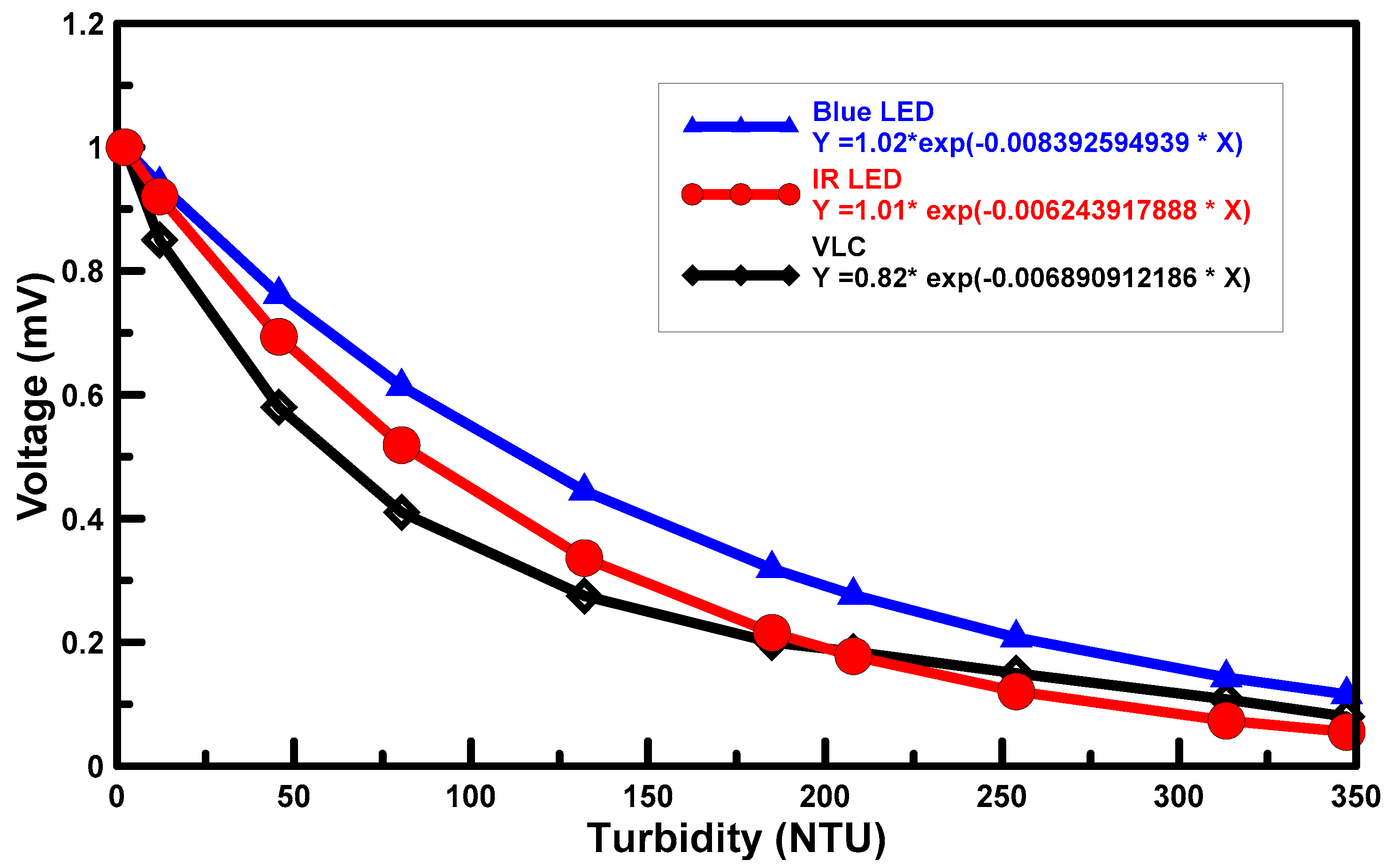
2.1. Water Turbidity Measurement

For water turbidity measurement, assume that $y_t$ is the sampled version of the received signal $y\left(t\right)$ at a sampling rate of $f_t$ and window size of $N_t$-point. The root mean square (RMS) value of $y_t$ can be computed as

$$y_{RMS}=\sqrt{\frac{y_t{y}_t^{\mathrm{T}}}{N_t}}$$

(3)

Assume that $y_0$ is the reference RMS value of transparent water. The difference between $y_{RMS}$ and $y_0$ can then be calculated as

$${\Delta }_{RMS}=y_0-y_{RMS}$$

(4)

Notably, Equation (4) is the attenuated power energy caused by the attenuated light path through the turbid water. The proposed system applies ${\Delta }_{RMS}$ to measure water turbidity.

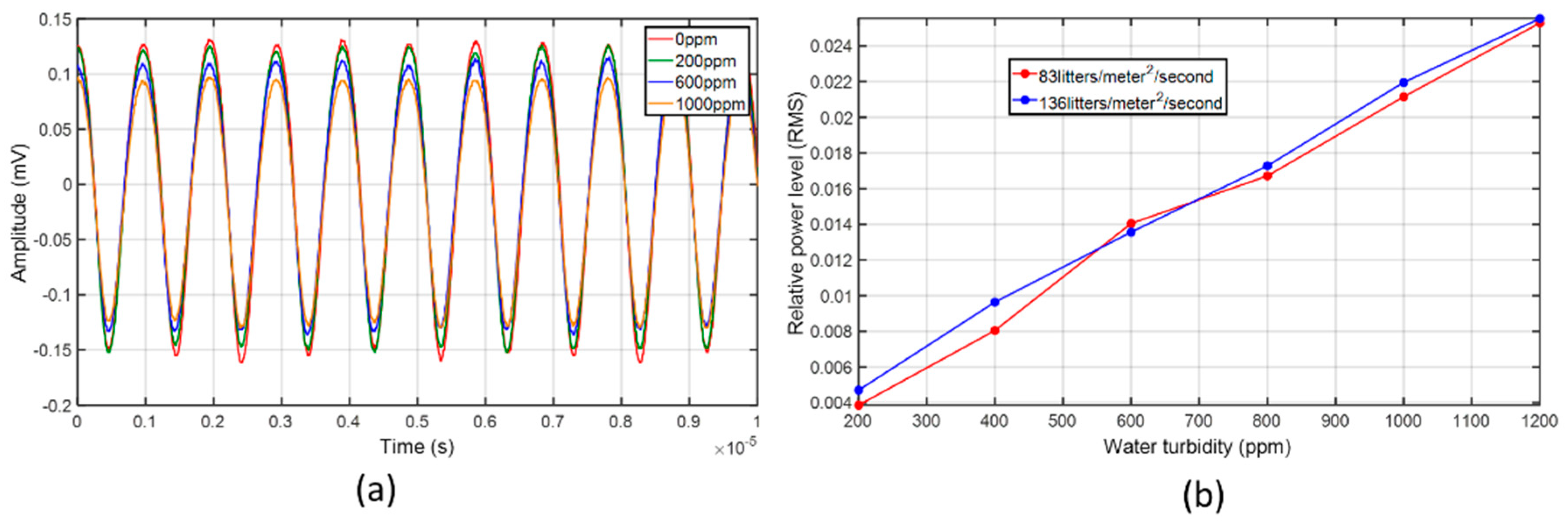
2.2. Water Flow Velocity Measurement

Figure 1 presents the signal processing setup for water flow velocity measurement, where $y_v=\left[y_{v,1},\dots ,y_{v,N_v}\right]$ is the sampled version of the received signal $y\left(t\right)$ at a sampling rate of $f_v$ and window size of $N_v$-point. The envelope of the received signal $y_v$ is computed to outline the characteristics of the signal. Let the Hilbert transform of $y_v$ be ${\tilde{y}}_v=\left[{\tilde{y}}_{v,1},\dots ,{\tilde{y}}_{v,N_v}\right]$. The envelope of the received signal $y_v$ can be expressed as

$${\widehat{y}}_v=\left[{\widehat{y}}_{v,1},\dots ,{\widehat{y}}_{v,N_v}\right]$$

(5)

in which ${\widehat{y}}_i=\sqrt{y_{v,i}^2+{\tilde{y}}_{v,i}^2},i=1,\dots ,N_v$. The frequency of the envelope from the received signal can be obtained as

$$y_F=\left[y_{F,1},\dots ,y_{F,N_v}\right]=\Im ({\widehat{y}}_v)$$

(6)

where $\Im (•)$ describes the Fourier transform operation. Herein, only half of $y_F$ is considered due to the symmetric property of the frequency response (i.e., $\left[y_{F,1},\dots ,y_{F,N_v/2}\right]$). To remove the direct current (DC), the system applies a frequency-domain DC-block filter with the coefficients

$$h_{DC}=\left[h_1,\dots ,h_{N_v/2}\right]$$

(7)

where $h_i=\{\begin{array}{l}1,i\ge p_{cut}\\ 0,i\le p_{cut}\end{array},i=1,\dots ,N_v/2.$

In Equation (7), $p_{cut}=\left[\left(f_v/2+f_{cut}\right)\left(N_v-1\right)/f_v+1\right]-N_v/2$, and $f_{cut}$ represents the DC-block filter of the desired cutoff frequency. The DC-block filter provides

$$y_{DC}=\left[y_{DC,1},\dots ,y_{DC,N_v/2}\right]$$

(8)

in which $y_{DC,i}=y_{F,i}{h}_i,i=1,\dots ,N_v/2.$

The Gaussian smoothing filter is applied to smooth the frequency response $y_{DC}$

$$y_G=y_{DC}\otimes g$$

(9)

where $g\hspace{0.17em}=\hspace{0.17em}{[\mathrm{g}}_1,\dots {,\mathrm{g}}_L]$ shows the L-point filter coefficients and ${\mathrm{g}}_i=e^{\left(-\frac{1}{2{\sigma }^2}\right)\left[(2/L-1\right)\left(i-1\right)-1{]}^2}, i=1, 2\dots L,$ herein, the $\mathsf{\sigma }$ contains the variance of the Gaussian coefficients. In the proposed system, the flowing velocity is measured from the frequency response in Equation (9).

Figure 2 depicts the experimental system for the water turbidity and water flow velocity measurement processes. The water flow was generated by a pump driven by a 1/6-hp motor in a 0.35 m wide and 2 m long flume. Four release holes were established at the end of the water channel to control the amount of water released. The sluice has been applied to the water flow channel to steadily control the water level of the flowing water. The turbidity of the flowing water was slight adding fine sand to the water. Sieving sediments of uniform sand with a diameter of 0.88 mm were used in this experiment. A 0.2 × 0.2 m pier made by a transparent acrylic column with VLC sensors was placed in the middle of the flume.

2.3. Experimental Setup for Water Turbidity Measurement

A sinusoidal signal with the frequency of 1 MHz was generated from the arbitrary waveform generator (AWG) in this turbidity measurement and stayed an amplitude of 0.2 V. The received signal was then obtained from the oscilloscope at a sampling rate of $f_t=1.024\hspace{0.17em}\mathrm{Ghz}$ with a window size of $N_t=\mathrm{10,240}$. From Equations (3) and (4), ${\Delta }_{RMS}$ values were computed. In this experiment, signal measurements were conducted at water turbidity levels of 0, 200, 400, 600, 800, 1000, and 1200 ppm and at two water flow velocities of 83.14q and 136.40q, where $q=\left(\mathrm{Liter}\right)/(\mathrm{second}\times {\mathrm{meter}}^2)$.

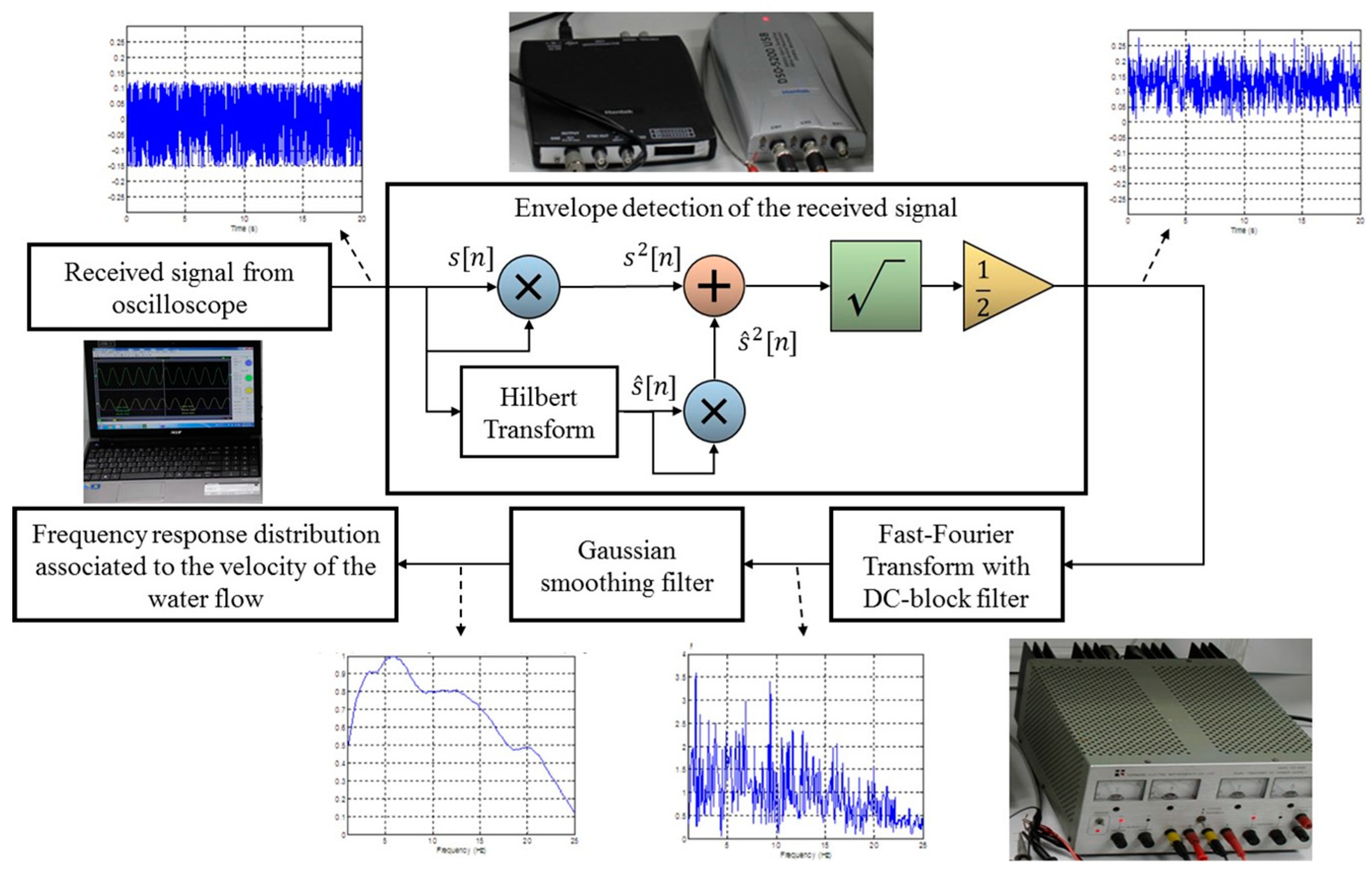
2.4. Experimental Setup for Water Flow Velocity Measurement

As mentioned, the sinusoidal signal was generated from the AWG. Signals were captured on the oscilloscope using a sampling rate of $f_v=50\hspace{0.17em}\mathrm{hz}$ with a window size of $N_v=500$ to estimate the flowing velocity. The envelope of the received signal ${\widehat{y}}_v$ was then calculated using Equation (5) and the DC-blocked frequency of the received signal $y_{DC}$ has computed from Equations (6)–(8). Finally, the Gaussian smoothing filter with a variance of $\sigma \hspace{0.17em}\hspace{0.17em}=\hspace{0.17em}\hspace{0.17em}1.8$ and a window size of $L=45$ was substituted into the smoothed frequency $y_G$ in Equation (9). The flowing velocities were set to be 25.98q, 83.14q, and 136.40q in the experiments.

Figure 3a shows the received signals at turbidity levels of 0, 200, 600, and 1000 ppm and at a water flow velocity of 83.14q. The attenuation of the amplitude of the received signals increased in accordance with the water turbidity levels. Figure 3b illustrates the relationship between ${\Delta }_{RMS}$ values and water turbidity levels at the water flow velocities of 83.14q and 136.40q. It seems that a linear relationship was observed between the ${\Delta }_{RMS}$ values and trifling water turbidity levels. Furthermore, ${\Delta }_{RMS}$ values computed at different flowing velocities were approximately the same. It shows that ${\Delta }_{RMS}$ is independent of the flowing velocity in the experiment.

Figure 4 shows the turbidity effect in nephelometric units (NTU) of the output voltage value for VLC, blue LED, and infrared LED (IR LED). VLC turbidity data was tested in the flowing flume with suspension particles distribution while the blue LED and IR LED turbidity data is obtained from the standard specimen. As shown in Figure 4, the VLC data have a slightly variated than the blue LED and IR LED, this variation is because the flowing suspension particles of the scattering, attenuation, and absorption effects have a significant influence on the measurement in the water. It is well-known that the on-line resolution of the experiment progress is highly dependent on the measurement angle of the sensor between the transmitter and the receiver. In addition, the ambient indoor light would be a noise resource which affects the performance of VLC during the experiment progress. Despite the influence of these factors, the nonlinear nature of turbidity which actually responds in exponential form to the light intensity was obviously obtained from the VLC monitoring system.

According to the results of the underwater turbidity and water flow velocity experiments in Section 2, we see that the communication light path of the VLC modules can be sensitively affected by turbulent movement of particles in water. In the following sections, the study further examines the effects of this notable phenomenon on real-time scour measurement by conducting real-time scour measurement and Hilbert transform analysis.

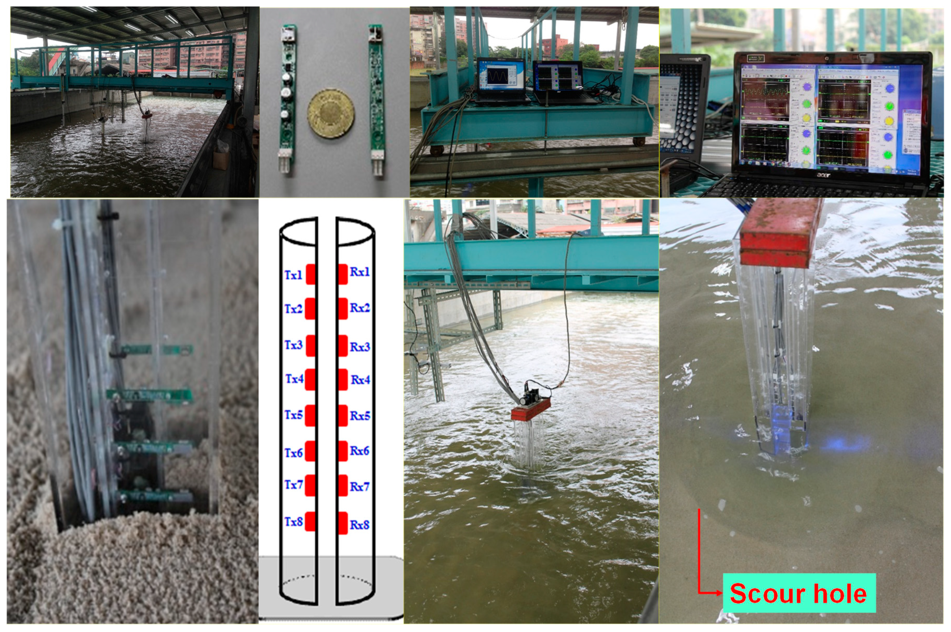
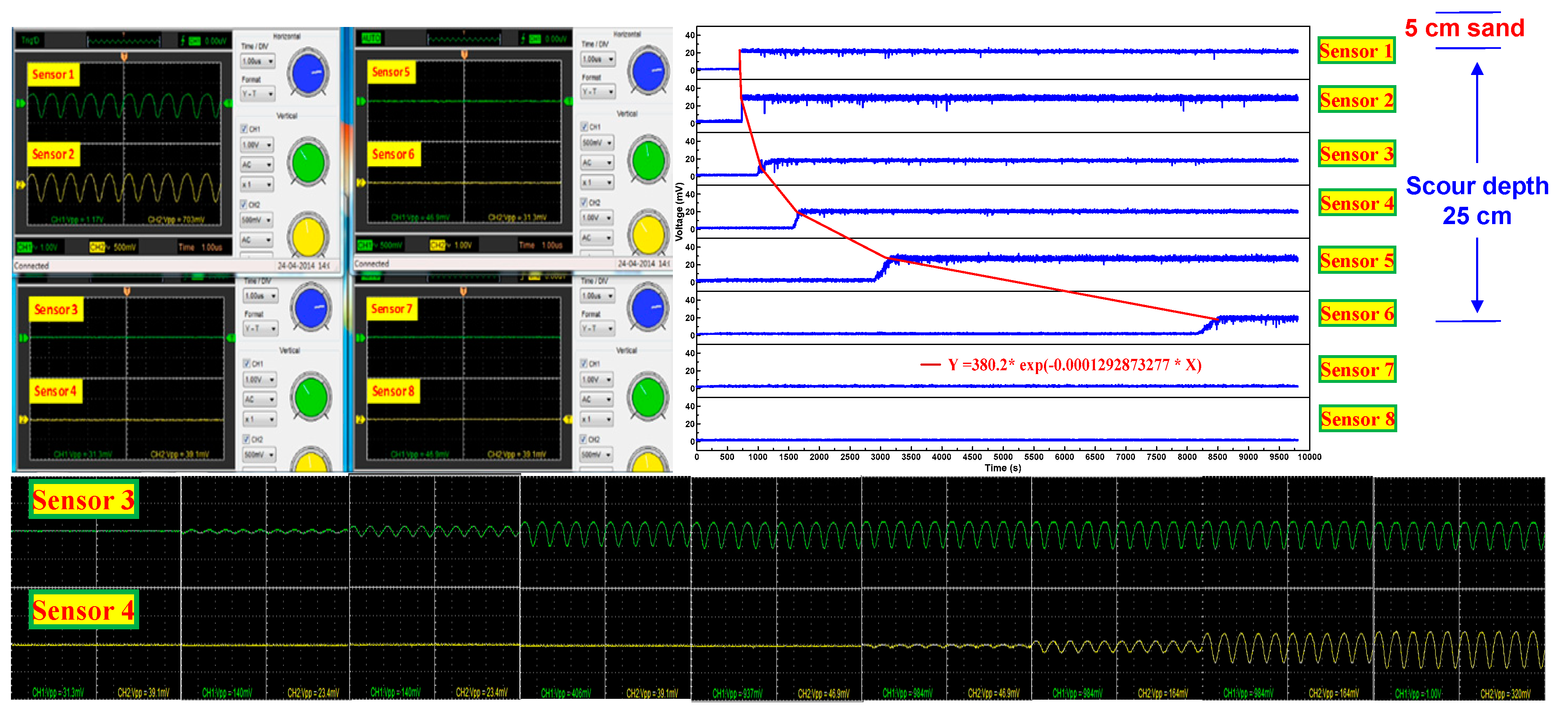
3. VLC Scour Experiment

An experiment was conducted in a 6 m wide and 30 m long flume, as depicted in Figure 5. Eight VLC sensors including the transmitter (Tx) and the receiver (Rx) were installed in the pier. Sensor 1 was located 5-cm below the bed surface. These sensors were arranged in two rows of eight sensors separated by 5-cm intervals in the vertical direction. The sampling rate was set to 100 Hz to record the time history throughout the scour experiment. Uniform sand with a diameter of 0.88 mm was paved as the bed material in the flume. The approach velocity of the steady current was set to be 0.5 m/s. All dynamic data were monitored through the experimental setup shown in Figure 5. Figure 5 illustrates the scour responses recorded by individual sensors. These responses were further analyzed using the proposed Hilbert–Huang transform (HHT) process.

Initially, all the sensors are embedded in the soil and the transmit signal cannot be detected by the receiver sensors. At the early stage, the scour depth increases significantly while inflow runs through the pier. As the embedded VLC sensor scoured from the soil due to scour, the significant signal of the waveform can be easily obtained. An obvious example of the sensors 3 and 4 is shown in Figure 6. The variation of waveform magnitude is due to the turbidity and velocity of the turbulent flow that contains time-depended suspension particles. As seen in Figure 6, the scour depth increases gradually after 1 h. Around 2.5 h, a total scour depth of 30 cm is measured in this test, which may be close to the equilibrium state. As experiment finished, the scour hole can be observed as shown in Figure 5. A small camera recorded the scouring process as a comparison to valid the scour depth evolution measured by the VLC. An empirical scour formula with the nonlinear nature of flowing water which responds in exponential form to the light intensity for the VLC monitoring system is also obtained as shown in Figure 6.

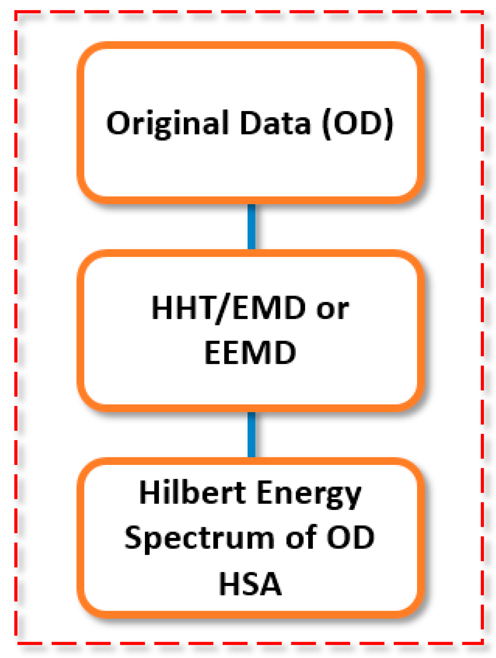
4. HHT and Data Analysis

4.1. Instantaneous Frequency

Traditionally, a Fourier spectrum is evaluated using sine and cosine basis functions with a fixed amplitude. However, signals vary with time limiting the applicability of the fast Fourier transform; moreover, obtaining the instantaneous frequency (IF) at any specific time is impractical. For a structure affected by an earthquake, understanding the frequency variation is imperative. The Hilbert transform is widely used for nonlinear and nonstationary cases, facilitating the analysis of a time-varying signal. A measured signal can be expressed in the form of a complex number to determine the instantaneous amplitude a(t) and instantaneous phase θ(t), and the IF ω(t) can then be determined [59,60]. The Hilbert transform can be defined as the convolution between X(t) and 1/t. For any time series $X\left(\tau \right)$, the Hilbert transform Y(t) can be expressed as

$$Y\left(t\right)=\frac{1}{\pi }P\underset{-\infty }{\overset{\infty }{{\displaystyle \int }}}\frac{X\left(\tau \right)}{t-\tau }d\tau$$

(10)

where P represents the Cauchy principal value.

Combining X(t) and Y(t) into a conjugate complex number yields an analytic signal Z(t)

$$Z(t)=X(t)+iY(t)=a(t)e^{i\theta (t)}$$

(11)

For example,

$$a(t)=\sqrt{X^2(t)+Y^2(t)}$$

(12)

$$\theta (t)={\tan }^{-1}\left(Y(t)/X(t)\right)$$

(13)

$$\omega (t)=\left(d\theta (t)/dt\right)$$

(14)

According to the analysis, the time–frequency–amplitude distribution of the time series can be obtained.

4.2. Empirical Mode Decomposition

In contrast to other decomposition methods, empirical mode decomposition (EMD) does not entail predetermining a basis function. In EMD, such a function is directly obtained from the signal data; therefore, this method has considerable flexibility. EMD entails decomposing an original signal into a finite number of intrinsic mode function (IMF) components; specifically, a signal is approximated as a sum of zero-mean amplitude modulation and frequency modulation components. The finite number of IMF components can be divided into high- and low-frequency partitions until a monotonic function (trend) remains. The original data can be regarded as the sum of all IMF components and trends. During analysis, if the time difference between the extreme values represents the time scalar of the intrawave, an optimal vibration modal resolution can be achieved and can be applied to nonzero mean values as well as non-zero-crossing data. Thus, the original signal can be re-presented as

$$X\left(t\right)={\displaystyle \sum }_{i=1}^n{c}_i+r_n$$

(15)

where $C_i$ is the ith intrinsic mode functions; $r_n$ is the residual.

4.3. Ensemble EMD

EMD is often used as a signal disassembly method. EMD is used to decompose mixed signals of different scales into different IMF components. However, a limitation of this approach is the phenomenon called ‘mode mixing’. Specifically, during the EMD process, a low-amplitude oscillation or an intermittent signal may exist in several IMF components; for example, a single modal component may be decomposed into different IMF components, or a single IMF component may contain two different modal signals, resulting in mode mixing within the IMF component. To solve this issue, Ensemble EMD (EEMD) is proposed [61]. When EEMD is performed, a white noise w_i(t) signal with a limited amplitude is added to the original signal X(t); thus, the original signal is transformed as

$$X_i(t)=X\left(t\right)+w_i\left(t\right)$$

(16)

4.4. Hilbert Spectrum

As indicated in Equation (17), an IMF component can be converted from a time-domain to a frequency-domain component; this process is called Hilbert spectral analysis (Figure 7)

$$X\left(t\right)={\displaystyle \sum }_{j=1}^n{a}_j\left(t\right) exp\left(i{\displaystyle \int }{\omega }_j\left(t\right)dt\right)$$

(17)

Although the Hilbert transform can process a monotonous trend and consider it a part of a longer amplitude, the remaining energy may be excessively strong, considering the uncertainties of longer-term trends and other low-energy elements and information contained in a high-frequency component. The preceding formula provides a time function for each amplitude and frequency component, and this formula can be expanded using a Fourier expression as

$$X\left(t\right)={\displaystyle \sum }_{j=1}^{\infty }{a}_j{e}^{i{\omega }_{j}t}$$

(18)

where a_j and w_j are constants. Comparing Equations (17) and (18) reveals that the IMF can be represented by a generalized Fourier expansion. Variables within the amplitude and the IF cannot only improve the expansion but also render it applicable to unsteady signals. In terms of the expansion of the IMF, the amplitude and the frequency modulation are clearly separated. The amplitude of the time function and the IF can be combined as the time–frequency–amplitude spectrum; this spectrum is referred to as the Hilbert amplitude spectrum.

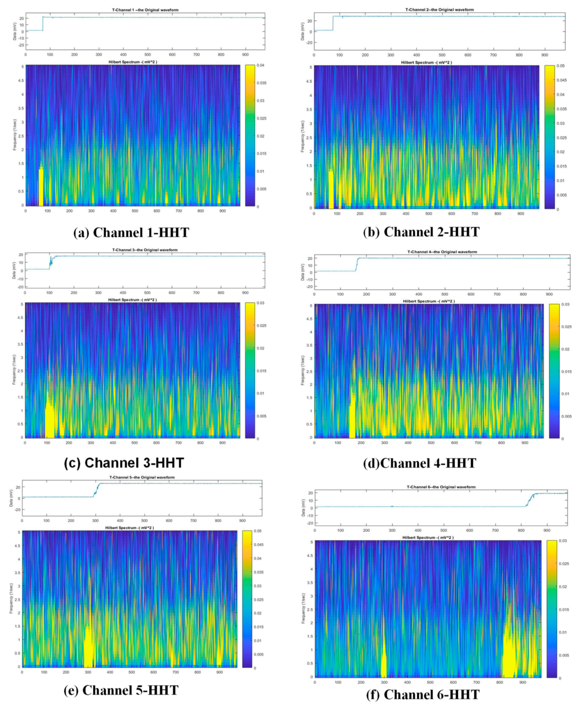
4.5. Analysis Results

From recorded data, the time history data and HHT diagrams obtained for the first six sensors are plotted in Figure 8. The recorded time history is plotted on the top of each subplot and the corresponding Hilbert amplitude spectrum is shown in the bottom. The time-varying IF demonstrated nonlinear characteristics of the signals. The x-axis represents the time history measured in seconds, and the energy density is illustrated at frequencies between 0 and 5 Hz, which contains the most energy of the vibration.

The HHT diagram for channel 1 shown in Figure 8a reveals a large energy distribution indicated by the significant yellow bar at approximately 90 s. This distribution can be attributed to the rapid jump in the time domain. Similarly, Figure 8b also reveals a yellow bar, indicating a sudden increase in the beginning of the time history. According to the color distribution in Figure 8b, more energy was covered in channel 2 than in channel 1, which fits well with the measured time histories.

The HHT diagrams for channels 3 and 4 shown in Figure 8c,d, respectively, reveal a gradual shift of the yellow bar, which indicates the large variation section of energy in the time domain. Based on the result, the yellow bars in HHT diagrams can be used to estimate the occurrence time of possible scour processes. Figure 8d indicates the scour phenomenon to occur between 150 and 200 s and then it continues till the end of the experiment; this figure also reveals the energy distribution in channel 4 to be greater than that in channel 3.

Finally, as observed from the time history, significant vibration can be reflected from channel 5. Furthermore, the HHT diagram for channel 5 shown in Figure 8e reveals that the yellow energy bar is shifted to 300 s. It can be treated as a proper indicator to evaluate the scour depth, which follows the trend observed from the experiment. Additionally, the HHT diagram for channel 6 shown in Figure 8f reveals two peaks. In contrast to the other five sensors, the first yellow energy bar located at 300 s with the fundamental frequency between 0 and 2 Hz is not considered as scour phenomenon in the HHT diagram. As only slight energy is shown in the diagram, it can be neglected as a small vibration in the time domain. By combining Figure 7 and Figure 8, a possible backbone scour curve can be established to provide a rapid estimation and early warning for scour processes around a bridge.

5. Summary

Offshore wind farms face more severe environmental conditions such as severe storms, typhoons, ocean currents, and waves. Flow induced scour around the foundation of structure is extremely complex. Scour leads to the excavation of sediments, reducing the safe capacity of the structures. The phenomenon of pier scour combines the effects of the vortex system involving time-dependent flow pattern and sediment transport mechanism. A real-time scour monitoring system can improve the safety of structures and afford cost-effective operations by preventing premature or unnecessary maintenance. Numerous studies have explored the mechanisms of hydraulic scour around foundations and have presented several formulas for scour depth estimation around piers. However, scour data from real-time monitoring systems are still inadequate due to the lack of reliable and durable instrumentation techniques.

Normally, water turbidity was measured based on absorption, attenuation, and scattering effects by using spectrometers or photometric devices. However, conventional estimation instruments are usually bulky and costly. Experimental results obtained in this study demonstrated the feasibility of the VLC modules for executing both water turbidity and water flow velocity measurements.

According to the results of the underwater turbidity and water flow velocity experiments, the communication light path of the VLC modules can be sensitively affected by turbulent movement of particles in water. These notable phenomenon effects could be further implemented as an early warning structural health monitoring system by conducting real-time scour measurement and Hilbert transform analysis. In this present study, an on-site scour monitoring system for offshore wind turbines has been proposed; specifically, the monitoring system consists of arrays of small VLC modules attached directly to a pile foundation structure and linked to a wireless network to enable remote data acquisition has demonstrated. From the flume experiment results, it revealed that the system was highly sensitive to seabed scour processes. The proposed robust sensory monitoring system has considered for further on-site applications and as an indicator to improve the empirical scour formulas for sustainable maintenance in the life cycle of offshore structures.

From the result analysis, the VLC ray is easily affected by the suspended particles in the water and the turbidity, especially in the scouring process. Hence, the proposed arrayed-transmission measurement method will be limited by the turbidity effect. In the future work, it may be necessary to cooperate with the reflection approach, as a supplement comparison, for simultaneous measuring the back-scattering characters. Combining these two transmission and back-scattering implementations would provide a better real-time approach to measure and discriminate turbidity, flow velocity, and scour depth. These data can be useful to establish a local scouring formula to evaluate structural safety.

References

1. Igwemeziea, V.; Mehmanparasta, A.; Koliosa, A. Current trend in offshore wind energy sector and material requirements for fatigue resistance improvement in large wind turbine support structures—A review. Renew. Sustain. Energy Rev. 2019, 101, 181–196. [Google Scholar] [CrossRef]
2. Willis, D.J.; Niezrecki, C.; Kuchma, D.; Hines, E.; Arwade, S.R.; Barthelmie, R.J.; DiPaola, M.; Drane, P.J.; Hansen, C.J.; Inalpolat, M.; et al. Wind energy research: State-of-the-art and future research directions. Renew. Energy 2018, 125, 133–154. [Google Scholar] [CrossRef]
3. Ma, H.; Yang, J.; Chen, L. Effect of scour on the structural response of an offshore wind turbine supported on tripod foundation. Appl. Ocean Res. 2018, 73, 179–189. [Google Scholar] [CrossRef]
4. Li, H.; Ong, M.C.; Leira, B.J.; Myrhaug, D. Effects of soil profile variation and scour on structural response of an offshore monopile wind turbine. J. Offshore Mech. Arct. Eng. 2018, 140, 042001. [Google Scholar] [CrossRef]
5. Chiew, Y.M.; Melville, B.W. Local scour around bridge piers. J. Hydraul. Eng. ASCE 1987, 25, 15–26. [Google Scholar] [CrossRef]
6. Melville, B.W.; Chiew, Y.M. Time scale for local scour at bridge piers. J. Hydraul. Eng. ASCE 1999, 125, 59–65. [Google Scholar] [CrossRef]
7. Melville, B.W. Pier and abutment scour: Integrated approach. J. Hydraul. Eng. ASCE 1997, 123, 125–136. [Google Scholar] [CrossRef]
8. Briaud, J.L.; Ting, F.C.K.; Chen, H.C. Erosion function apparatus for scour rate predictions. J. Geotech. Geoenviron. Eng. 2001, 127, 105–113. [Google Scholar] [CrossRef]
9. Briaud, J.L.; Ting, F.C.K.; Chen, H.C. SRICOS: Prediction of scour rate in cohesive soils at bridge piers. J. Geotech. Geoenviron. Eng. 1999, 125, 237–246. [Google Scholar] [CrossRef]
10. Shirole, A.M. Bridge management to the Year 2020 and beyond. Transp. Res. Rec. 2010, 2202, 159–164. [Google Scholar] [CrossRef]
11. Lagasse, P.F.; Richardson, E.V. ASCE compendium of stream stability and bridge scour papers. J. Hydraul. Eng. ASCE 2001, 127, 531–533. [Google Scholar] [CrossRef]
12. Wardhana, K.; Hadipriono, F.C. Analysis of recent bridge failures in the United States. J. Perform. Constr. Facil. 2003, 17, 144–150. [Google Scholar] [CrossRef]
13. Roulund, A.; Sumer, B.M.; Fredsoe, J. Numerical and experimental investigation of flow and scour around a circular pile. J. Fluid Mech. 2005, 534, 351–401. [Google Scholar] [CrossRef]
14. Lin, Y.B.; Chen, J.C.; Chang, K.C. Real-time monitoring of local scour by using fiber Bragg grating sensors. Smart Mater. Struct. 2005, 14, 664–670. [Google Scholar] [CrossRef]
15. Lin, Y.B.; Lai, J.S.; Chang, K.C. Flood scour monitoring system using fiber Bragg grating sensors. Smart Mater. Struct. 2006, 15, 1950–1959. [Google Scholar] [CrossRef]
16. Lin, Y.B.; Lai, J.S.; Chang, K.C.; Chang, W.Y.; Lee, F.Z.; Tan, Y.C. Using MEMS sensors in the bridge scour monitoring system. J. Chin. Inst. Eng. 2010, 33, 25–35. [Google Scholar] [CrossRef]
17. Prendergast, L.J.; Gavin, K. A review of bridge scour monitoring techniques. J. Rock Mech. Geotech. Eng. 2014, 6, 138–149. [Google Scholar] [CrossRef]
18. Luengo, J.; Negro, V.; Garcia-Barba, J. New detected uncertainties in the design of foundations for offshore Wind Turbines. Renew. Energy 2019, 131, 667–677. [Google Scholar] [CrossRef]
19. Oliveira, G.; Magalhaes, F.; Cunha, A. Vibration-based damage detection in a wind turbine using 1 year of data. Struct. Control Health Monit. 2018, 25, 1–22. [Google Scholar] [CrossRef]
20. Prendergast, L.J.; Gavin, K.; Doherty, P. An investigation into the effect of scour on the natural frequency of an offshore wind turbine. Ocean Eng. 2015, 101, 1–11. [Google Scholar] [CrossRef] [Green Version]
21. Tseng, W.C.; Kuo, Y.S.; Lu, K.C.; Chen, J.W.; Chung, C.F.; Chen, R.C. Effect of scour on the natural frequency responses of the meteorological mast in the Taiwan Strait. Energies 2018, 11, 823. [Google Scholar] [CrossRef]
22. Tseng, W.C.; Kuo, Y.S.; Chen, J.W. An investigation into the effect of scour on the loading and deformation responses of monopile foundations. Energies 2017, 10, 1190. [Google Scholar] [CrossRef]
23. Chen, W.I.; Wong, B.L.; Lin, Y.H.; Chau, S.W.; Huang, H.H. Design and analysis of jacket substructures for offshore wind turbines. Energies 2016, 9, 264. [Google Scholar] [CrossRef]
24. Yang, W.; Tian, W. Concept research of a countermeasure device for preventing scour around the monopole foundations of offshore wind turbines. Energies 2018, 11, 2593. [Google Scholar] [CrossRef]
25. Yu, T.; Lian, J.; Shi, Z. Experimental investigation of current-induced local scour around composite bucket foundation in silty sand. Ocean Eng. 2016, 117, 311–320. [Google Scholar] [CrossRef]
26. Esteban, M.D.; Counago, B.; Lopez-Gutierrez, J.S. Gravity based support structures for offshore wind turbine generators: Review of the installation process. Ocean Eng. 2015, 110, 281–291. [Google Scholar] [CrossRef]
27. McGovern, D.J.; Ilic, S.; Folkard, A.M. Time development of scour around a cylinder in simulated tidal currents. J. Hydraul. Eng. 2014, 140, 04014014. [Google Scholar] [CrossRef]
28. Michalis, P.; Saafi, M.; Judd, M. Capacitive sensors for offshore scour monitoring. Proc. Inst. Civ. Eng. Energy 2013, 166, 189–196. [Google Scholar] [CrossRef]
29. Harris, J.M.; Whitehouse, R.J.S.; Benson, T. The time evolution of scour around offshore structures. Proc. Inst. Civ. Eng. Energy Marit. Eng. 2010, 163, 3–17. [Google Scholar] [CrossRef] [Green Version]
30. Ong, M.C.; Trygsland, E.; Myrhaug, D. Numerical study of seabed boundary layer flow around monopile and gravity-based wind turbine foundations. J. Offshore Mech. Arct. Eng. 2017, 139, 042001. [Google Scholar]
31. Oh, K.Y.; Nam, W.; Ryu, M.S.; Kim, J.Y.; Epureanu, B.I. A review of foundations of offshore wind energy convertors: Current status and future perspectives. Renew. Sustain. Energy Rev. 2018, 88, 16–36. [Google Scholar] [CrossRef]
32. Guan, D.W.; Chiew, Y.M.; Melville, B.W.; Zheng, J.H. Current-induced scour at monopile foundations subjected to lateral vibrations. Coast. Eng. 2019, 144, 15–21. [Google Scholar] [CrossRef]
33. Petersen, T.U. Scour around Offshore Wind Turbine Foundations. Ph.D. Thesis, Technical University of Denmark, Lyngby, Denmark, 2014. [Google Scholar]
34. Prendergast, L.J.; Reale, C.; Gavin, K. Probabilistic examination of the change in eigen frequencies of an offshore wind turbine under progressive scour incorporating soil spatial variability. Mar. Struct. 2018, 57, 87–104. [Google Scholar] [CrossRef]
35. Rivier, A.; Bennis, A.C.; Pinon, G.; Magar, V.; Gross, M. Parameterization of wind turbine impacts on hydrodynamics and sediment transport. Ocean Dyn. 2016, 66, 1285–1299. [Google Scholar] [CrossRef] [Green Version]
36. Nielsen, A.W.; Liu, X.F.; Sumer, B.M.; Fredsoe, J. Flow and bed shear stresses in scour protections around a pile in a current. Coast. Eng. 2013, 72, 20–38. [Google Scholar] [CrossRef]
37. Riahi-Madvar, H.; Dehghani, M.; Seifi, A.; Salwana, E.; Shamshirband, S.; Mosavi, A.; Chau, K.W. Comparative analysis of soft computing techniques RBF, MLP, and ANFIS with MLR and MNLR for predicting grade-control scour hole geometry. Eng. Appl. Comput. Fluid Mech. 2019, 13, 529–550. [Google Scholar] [CrossRef] [Green Version]
38. Khan, M.; Tufail, M.; Azamathulla, H.M.; Ahmad, I.; Muhammad, N. Genetic functions-based modelling for pier scour depth prediction in coarse bed streams. Proc. Inst. Civ. Eng. Water Manag. 2018, 171, 225–240. [Google Scholar] [CrossRef]
39. Ebtehaj, I.; Bonakdari, H.; Moradi, F.; Gharabaghi, B.; Khozani, Z.S. An integrated framework of Extreme Learning Machines for predicting scour at pile groups in clear water condition. Coast. Eng. 2018, 135, 1–15. [Google Scholar] [CrossRef]
40. Eghbalzadeh, A.; Hayati, M.; Rezaei, A.; Javan, M. Prediction of equilibrium scour depth in uniform non-cohesive sediments downstream of an apron using computational intelligence. Eur. J. Environ. Civ. Eng. 2018, 22, 28–41. [Google Scholar] [CrossRef]
41. Chou, J.S.; Pham, A.D. Nature-inspired metaheuristic optimization in least squares support vector regression for obtaining bridge scour information. Inf. Sci. 2017, 399, 64–80. [Google Scholar] [CrossRef]
42. Ebtehaj, I.; Sattar, A.M.A.; Bonakdari, H.; Zaji, A.H. Prediction of scour depth around bridge piers using self-adaptive extreme learning machine. J. Hydroinform. 2017, 19, 207–224. [Google Scholar] [CrossRef]
43. Lashkar-Ara, B.; Ghotbi, S.M.H.; Najafi, L. Prediction of scour in plunge pools below outlet bucket using artificial intelligence. KSCE J. Civ. Eng. 2016, 20, 2981–2990. [Google Scholar] [CrossRef]
44. Mesbahi, M.; Talebbeydokhti, N.; Hosseini, S.A.; Afzali, S.H. Gene-expression programming to predict the local scour depth at downstream of stilling basins. Sci. Iran. 2016, 23, 102–113. [Google Scholar] [CrossRef] [Green Version]
45. Choi, S.U.; Choi, B.; Choi, S. Improving predictions made by ANN model using data quality assessment: An application to local scour around bridge piers. J. Hydroinform. 2015, 17, 977–989. [Google Scholar] [CrossRef]
46. Hosseini, R.; Amini, A. Scour depth estimation methods around pile groups. KSCE J. Civ. Eng. 2015, 19, 2144–2156. [Google Scholar] [CrossRef]
47. Cheng, M.Y.; Cao, M.T. Hybrid intelligent inference model for enhancing prediction accuracy of scour depth around bridge piers. Struct. Infrastruct. Eng. 2015, 11, 1178–1189. [Google Scholar] [CrossRef]
48. Turan, K.H.; Yanmaz, A.M. Reliability-based optimization of river bridges using artificial intelligence techniques. Can. J. Civ. Eng. 2011, 38, 1103–1111. [Google Scholar] [CrossRef]
49. Zounemat-Kermani, M.; Teshnehlab, M. Using adaptive neuro-fuzzy inference system for hydrological time series prediction. Appl. Soft Comput. 2008, 8, 928–936. [Google Scholar] [CrossRef]
50. Komine, T.; Nakagawa, M. Fundamental analysis for visible-light communication system using LED lights. IEEE Trans. Consum. Electron. 2004, 50, 100–107. [Google Scholar] [CrossRef]
51. Zhang, Y.; Stritlien, K.; Bellingham, J.G.; Baggeroer, A.B. Acoustic doppler velocimeter flow measurement from an autonomous underwater vehicle with applications to deep ocean convection. J. Atmos. Ocean. Technol. 2001, 18, 2038–2051. [Google Scholar] [CrossRef]
52. Nezu, I.; Rodi, M.A.W. Open-channel flow measurements with a laser doppler anemomter. J. Hydraul. Eng. 1986, 112, 335–355. [Google Scholar] [CrossRef]
53. Kocsis, L.; Herman, P.; Eke, A. The modified Beer-Lambert law revisited. Phys. Med. Biol. 2006, 51, 91–98. [Google Scholar] [CrossRef]
54. Zeng, Z.; Fu, S.; Zhang, H.; Dong, Y.; Cheng, J. A Survey of Underwater Wireless Optical Communication. IEEE Commun. Surv. Tutor. 2017, 19, 204–238. [Google Scholar] [CrossRef]
55. Wang, C.; Yu, H.Y.; Zhu, Y.J. A long distance underwater visible light communication system with single photon avalanche diode. IEEE Photonics J. 2016, 8, 7906311. [Google Scholar] [CrossRef]
56. Al-Kinani, A.; Wang, C.X.; Zhou, L.; Zhang, W. Optical wireless communication channel measurements and models. IEEE Commun. Surv. Tutor. 2018, 20, 1939–1962. [Google Scholar] [CrossRef]
57. Kaushal, H.; Kaddoum, G. Underwater Optical Wireless Communication. IEEE Access 2016, 4, 1518–1547. [Google Scholar] [CrossRef]
58. Chang, C.C.; Wu, C.T.; Lin, Y.B.; Gu, M.H. Water velocimeter and turbidity-meter using visible light communication modules. In Proceedings of the Sensors, 2013 IEEE, Baltimore, MD, USA, 3–6 November 2013. [Google Scholar]
59. Huang, N.E.; Shen, Z.; Long, S.R.; Wu, M.C.; Shih, S.H.; Zheng, Q.; Tung, C.C.; Liu, H.H. The empirical mode decomposition method and the Hilbert spectrum for non-stationary time series analysis. Proc. R. Soc. Lond. A 1998, 454, 903–995. [Google Scholar] [CrossRef]
60. Su, S.C.; Wen, K.L.; Huang, N.E. A New Dynamic Building Health Monitoring Method Based on the Hilbert-Huang Transform. Terr. Atmos. Ocean. Sci. 2014, 25, 289–318. [Google Scholar] [CrossRef]
61. Wu, Z.H.; Huang, N.E. Ensemble Empirical Mode Decomposition: A Noise-Assisted Data Analysis Method. Adv. Adapt. Data Anal. 2009, 1, 1–41. [Google Scholar] [CrossRef]
Figure 1. Flowchart of signal processing for water flow velocity/turbidity measurement.
Water 11 01486 g001
Figure 2. Experimental setup consisting of A: VLC sensor (Tx & Rx); B, C, D: waveform signal generator; E: input waveform signal monitoring; F: sensor signal response monitoring.
Water 11 01486 g002
Figure 3. (a) Received signals at turbidity levels of 0, 200, 600, and 1000 ppm and at water a flow velocity of 83.14q; (b) water turbidity levels versus Δ R M S values.
Water 11 01486 g003
Figure 4. Turbidity effect in nephelometric units (NTU).
Water 11 01486 g004
Figure 5. Hydraulic flume test and experimental setup.
Water 11 01486 g005
Figure 6. Monitoring interface and recorded scour responses.
Water 11 01486 g006
Figure 7. HHT calculation process.
Water 11 01486 g007
Figure 8. HHT diagrams for the first six sensors.
Water 11 01486 g008