Article

Influencing Factors of the Spatial–Temporal Variation of Layered Soils and Sediments Moistures and Infiltration Characteristics under Irrigation in a Desert Oasis by Deterministic Spatial Interpolation Methods

1
Key Laboratory of Subsurface Hydrology and Ecological Effects in Arid Region, Ministry of Education, College of Environmental Science and Engineering, Chang’an University, Xi’an 710016, China
2
River Engineering and Technology Research Center of Shaanxi Province, Xi’an 710016, China
3
School of Geological Engineering and Surveying, Chang′an University, Xi’an 710016, China
4
School of Tourism and Resources Environment, Qiannan Normal University for Nationalities, Duyun 558000, China
*
Author to whom correspondence should be addressed.
Water 2019, 11(7), 1483; https://doi.org/10.3390/w11071483
Submission received: 30 May 2019 / Revised: 10 July 2019 / Accepted: 14 July 2019 / Published: 17 July 2019
(This article belongs to the Special Issue Assessment of Spatial and Temporal Variability of Water Resources)

Abstract

:
Soil moisture is the main limiting factor for crop growth and the sustainable development of oases in arid desert areas. Therefore, the temporal and spatial variation and infiltration laws of oasis soil moisture should be studied. The objective of this study is to reveal the influencing factors of the spatial–temporal variation of layered soil and sediment moisture and infiltration characteristics under irrigation in desert oases. Hydraulic conductivities were measured using the double-ring infiltrometer, while the regional and site soil moistures were measured and calibrated using weighted method and neutron moisture meter. Deterministic spatial interpolation methods, including multiquadric radial basis function, inverse distance weighted, and local polynomial regression isogram, were adopted to map the regional distribution of hydraulic conductivities, spatial soil moistures, and spatial–temporal isogram of the point site soil moistures in Yaoba Oasis, respectively. Results showed that the leading influencing factors of the (1) regional spatial soil moisture were soil and sediment permeability, stream link direction, microclimate, and dewfalls; (2) spatial layered soil and sediment moistures were microclimate and dew condensation; and (3) spatial–temporal variation at the point site profiles were soil texture, water requirement, and preferential flow. Under irrigation, soil moisture increased significantly, in which the maximum increase was 10.8 times the original state, while the recharging depth substantially increased up to 580 cm with the preferential flow. The spatial–temporal variation of the soil moisture under irrigation indicated that the best irrigation frequency should be 15 days per time. Moreover, the infiltration process can be divided into the preferential flow, piston flow, and balanced infiltration stages.

Graphical Abstract

1. Introduction

Oasis is the most frequent and active region of human activities in arid areas in the world [1], such as the Middle East, Mexico, most parts of Africa, parts of northwestern America, and pockets of India, Central Asia, and northwestern China [2]. Oasis is also the guarantee and support of the opening up and cooperation of the social and economic development along the Silk Road [3,4]. The development and evolution of oasis mainly depends on ground water supply due to the extreme scarcity of surface water resources [5,6,7]. Soil moisture is the main limiting factor for the growth and sustainability of oasis agriculture. Hence, studying the temporal and spatial variation characteristics of soil moisture is of considerable importance to understand the agricultural irrigation regime and provide further scientific basis for the development of oasis agriculture [8,9].
Numerous investigations have been conducted on oasis soil moisture in terms of the following three aspects: (1) the relationships between soil moisture and groundwater dynamics [10,11,12,13], soil salinization [14,15,16], vegetation, and land use pattern [17,18,19]; (2) the spatial–temporal variation and temporal stability of soil moisture in oases [20,21,22,23,24,25]; and (3) the study of soil water infiltration characteristics and migration laws [26].
However, with regard to the second aforementioned aspect, previous research on the spatial–temporal variation and temporal stability of soil moisture either simply focused on studying the soil moisture content of a certain layer or depth fluctuating with time series [20,21,27], or of a certain time variation along the soil layers or depths [27,28,29], respectively. Determining the continuity of temporal and spatial changes of soil moisture is difficult. Soil moisture, which might be affected by environmental factors, such as precipitation, evapotranspiration [30], irrigation, groundwater table fluctuation, soil texture, and soil bulk density, continuously changes with time and depth [31]. Therefore, an integrated method is urgently needed to comprehensively and simultaneously combine the spatial and temporal variations of soil moisture. Fortunately, Zhou et al. [32] proposed the polynomial regression isogram (PRI) method to describe the spatial–temporal variation of soil moisture on the basis of a time isogram method. The regression isogram is informative, remarkable, intuitive, and reliable; it also facilitates convenient analysis to reveal the variation of soil moisture from surface to deep layers in a certain period [33]. In the application of PRI in previous research [32,33], the studied soil profiles were all relatively uniform on soil texture, which can be well described by PRI in terms of the overall distribution and variation trend of the soil moisture. When investigating the layered soil profile, the heterogeneity of soil moisture should be considered. Therefore, the local polynomial regression isogram (LPRI) method should be adopted to address the heterogeneity and complexity of soil moisture induced by the diversity of profile texture.
With respect to the third aspect, the previous studies on soil water transportation were mainly based on uniform flow theory, and only a few ones were considered preferential flow [34,35]. Oases are often located in arid areas with windy weather, unevenly distributed precipitation, and large temperature differences in a day/night as well as during an inter-annual period [1]. The typical climate facilitates the production of macropores and fissures through dry and wet cycles, alternate freezing and thawing, crop roots, and soil animal activities, which provides dominant channels for rainfall and irrigation water prone to the induction of preferential flow [35]. Therefore, the infiltration forms of rainfall and irrigation water mainly include piston flow (balanced flow) and preferential flow (non-uniform flow) [36]. Piston flow is characterized by the downward migration of the infiltrated soil moisture due to the newly infiltrated soil water, showing a uniform wetting front. By contrast, preferential flow is the migration of the soil water along the dominant infiltration pathways, such as dead root pores, soil fauna burrows, fissures, and wetting–drying or freezing–thawing cycle cracks [37], to bypass the soil matrix through quick penetration into deep soil [38] and facilitate the induction of excessive infiltration and preferential flow [39]. Yan et al. [34] studied the response of preferential flow to irrigation and found that the preferential flow induced by ant burrows and crop roots exerted considerable influence on the infiltration depth. Sun et al. [40] used dye tracing and image processing to study the relationship between soil macropores and preferential flow, indicating that the preferential flow induced by soil macropores increased the soil water infiltration rate by 1.48 times. Ivanov et al. [37] discussed the applications of X-ray computed tomography (X-ray CT) in soil science and found that X-ray CT could effectively help to visualize the three-dimensional pore structures to acquire the parameters (pore diameter, volume, shape, orientation, connectivity, tortuosity, coordinate (contact) numbers, porosity, pore size distribution etc.) and even to calculate and simulate the permeability [41] or the water retention curve [42] of the soil with pores and fissures, thereby having significant hydraulic importance to reveal the laws of soil water movement. Zhang et al. [43] and Zhang et al. [44] investigated the susceptibility of macropore flow in different cultivating years and found that an old oasis (cultivated for more than 50 years) is prone to facilitate macro flow. The Yaoba Oasis studied in this work belongs to the old one. Therefore, this oasis is of high susceptibility to preferential flow, that is, preferential flow is the main infiltration form of soil water recharging in Yaoba Oasis. All the aforementioned research suggested that preferential flow has an important influence on the infiltration depth, seepage velocity, and irrigation response in oases due to its rapid and non-uniform infiltration characteristics. However, none of these studies discussed the influence of preferential flow on the spatial distribution and temporal stability of soil moisture.
In summary, an existing gap was found in the aforementioned literature review. Thus, this study has the following objectives: (1) to explore the influencing factors of the spatial and vertical distribution of the soil and sediment moistures in Yaoba Oasis; (2) to reveal the influencing factors of the spatial–temporal variation of the layered soil moistures at the point site profiles by considering preferential flow along the depths and time series; and (3) to clarify the infiltration pattern and stage characteristics on the consideration of preferential flow. High-resolution monitoring of soil moisture was performed once per 12 h, and the intervals of 20–50 cm along the profiles were measured by the neutron moisture meter to meet the aforementioned objectives. The LPRI was used to map the isogram of soil moisture to clearly reflect the variation with time and soil depth. Based on the isogram, the influence of preferential flow on the spatial–temporal variation of the soil and sediment moisture was discussed.

2. Materials and Methods

2.1. Study Area

This study was conducted at some patches of arable land within the Yaoba Oasis (105°34′–105°39′ E, 38°25′–38°36′ N) in the Alxa Left Banner, Inner Mongolia, China. The study area, which is located between the Helan Mountain in the east and Tengger Desert in the west, has an area of 81.2 km2 (Figure 1). The terrain is high in the east and low in the west with an elevation of 1290–1342 m and an average slope of 1°. The weather is a typical arid desert climate type. The average annual precipitation is 198.0 mm, and the average annual evaporation is 2394 mm (11.5 times the precipitation). The precipitation is mainly distributed from July to September, accounting for more than 65% of the total annual precipitation, while the maximum evaporation occurs in May to July, accounting for 45% of the total annual amount. The precipitation is decreased from east to west due to the effect of Helan Mountain and Tengger Desert. The annual precipitation is more than 400 mm near the eastern Helan Mountains and less than 150 mm near the edge of the western desert. The soil types of the study area are mainly gray desert soil, desert solonchaks, and aeolian sandy soil. Despite the presence of eight ditches in front of Helan Mountain (on the east side of oasis), the surface water resources of Yaoba Oasis are scarce because most of the ditches come from seasonal intermittent water flow only during the occurrence of heavy rains or storms in June to September. The agriculture in the oasis is maintained by groundwater irrigation due to the lack of surface water. At present, more than 60,000 mu (1 mu = 0.0667 ha = 666.7 m²) of farmland is available, and the annual irrigation water is even 600–700 m3/mu. The irrigation activities are usually conducted during winter, summer, and autumn. In terms of extensive flood irrigation, the oasis faces many problems, such as groundwater over-exploitation, soil salinization, vegetation degradation, ground fissures, and land subsidence.

2.2. Test Design and Datasets

2.2.1. Point Layout and In Situ Tests

A total of 21 test points were set with the density of one point per geographic grid (2 × 2 km) by ArcGIS 10.3.1 (Esri Inc., Redlands, CA, USA) to understand the spatial distribution and variation law of soil moisture of Yaoba Oasis (Figure 1). Each test point was positioned using a handheld GPS. The points were adjusted and set according to the actual land features under the reference of the geographic grids. An in-situ infiltration test was conducted near each test point using the double-ring infiltration test to obtain the soil hydraulic conductivity (K, m/day) that was calculated using the principle of Darcy’s law as used in References [45,46]. Based on the infiltration tests, the distribution of hydraulic conductivities was mapped by Multiquadric Radial Basis Function (MRBF, introduced in Section 2.3.1) in ArcGIS showing in Figure 2. Among the 21 test points, three points were selected to conduct the field irrigation test.
To observe the temporal stability along profiles of soil moisture and reveal the influence of irrigation activities on the temporal stability, observation holes were drilled to the depth of 400–600 cm and stainless steel access tubes (with inner diameter of 50 mm and tube wall thickness of 2 mm) were installed at the selected points for soil observation by the neutron moisture meter (Model number: L520, Institute of Atomic Energy, Jiangsu Academy of Agricultural Sciences). Referring to Figure 2, the selected points were points 4 (4#, k = 0.66 m/d) and 9 (9#, k = 0.53 m/d) with moderate infiltration capacity and point 17 (17#, k = 1.63 m/d) with strong infiltration capacity. The 4# test point was located at a vegetable patch planted with edamame, and two observation holes (marked as 4#1 and 4#2) were dug to the depth of 425 cm to measure the soil moisture using the neutron moisture meter. The 9# test point was located at an arable land planted with high water consumption corn, and three observation holes (marked as 9#1, 9#2, and 9#3) were dug to the depth of 580 cm, 580 cm, and 480 cm to measure the soil moisture using the neutron moisture meter. The 17# test point was located at an arable land planted with water-saving millet, and three observation holes (marked as 17#1, 17#2 and 17#3) were dug to the depth of 480 cm, 500 cm, and 500 cm to measure the soil moisture using the neutron moisture meter.

2.2.2. Sampling and Measurement of Soil Physical Properties

On the basis of our previous studies [26,46], disturbed soil samples were collected at an interval of 20 and 50 cm within the depth of 0–100 and 100–600 cm, respectively, while punching the observation holes. Two sets of samples at each sampling interval were collected in sealable plastic bags and aluminum boxes for the measurement of soil particle composition and initial moisture content, respectively. More importantly, samples should be increased when the lithology changes at the current sampling layer. The wet weight of the collected soil samples was immediately measured and recorded in situ. In addition, a 6-m-deep test pit was dug, and 30 intact soil samples were collected via cutting-ring method to measure soil bulk density. The soil particle composition was measured by the Bettersize 2000 laser particle size analyzer (Dandong Bettersize Instruments Ltd., Dandong, China), and the soils and sediments of each layer were named according to the soil texture classification standard of the US Department of Agriculture (USDA) (Figure 3). Simultaneously, the bulk density and initial moisture content of the soil samples were respectively determined by the cutting-ring and oven-drying method. The physical properties of the soil are shown in Table A1.

2.2.3. Calibration of Neutron Moisture Meter and Observation Schedule of the Soils and Sediments Moistures

The soil and sediment moisture contents of the test point profiles were determined using the neutron moisture meter, which comprises a fast neutron source, a slow neutron detector, a counter, a shielded crucible, and a hard tube. The basic principle is to count the slow neutrons caused by the collision between fast neutrons and hydrogen nuclei in the soil water. The counting rate of slow neutrons is proportional to the soil volumetric moisture content, which can be estimated by measuring the number of slow neutrons reflected by the soil per unit time as shown below [28]:
θ V =   a r n + b
where: θ V is the volumetric water content, cm3/cm3; a and b are calibration coefficients of the neutron method to determine the moisture content; and r n is the relative counting rate of the neutron moisture meter. r n = C n / C s , where C n is the actual reading of the neutron moisture meter, and C s is the standard count (the standard readings of the moisture meter in pure water or in the indoor protective layer at the temperature of 25 °C). θ V = θ M ×   r s , where θ M is the initial mass moisture content, which can be determined by the indoor drying method, and r s is the soil bulk density.
Given that C s can be considered as a fixed value under the same conditions, the neutron moisture meter calibration equation is expressed as follows:
θ V = a C n + b
Figure 3 shows the different textures of the layers along vertical profiles. The neutron moisture meter data were calibrated as piecewise linear equations (Table 1) of the different depths of each layer of observation point. Based on the piecewise grading formula, the soil and sediment moisture contents of each layer at each point were derived, and the soil moisture dynamic monitoring of typical oasis patches was conducted.
The observation period is from 9 August to 11 September 2015. Two irrigation activities with intervals of approximately 16–19 days were observed during this period mainly to reveal the infiltration characteristics along the profiles. The schedule of each point is shown in Table 2. At the beginning of the irrigation period, the soil and sediment moisture contents were observed twice a day (morning and afternoon) using the neutron moisture meter. After the data stabilized, the observation was changed to once a day. According to Reference [47], the irrigation water requirements of the whole growth period of corn, edamame, and millet are 660 m3/mu, 450 m3/mu, and 380 m3/mu, respectively. In this study, amounts of the two irrigations of points 4, 9 and 17 were all 100 m3/mu, 120 m3/mu and 70 m3/mu, respectively. The irrigation methods were all flood irrigation.

2.3. Deterministic Spatial Interpolation Methods

2.3.1. MRBF

There are many deterministic interpolation methods in ArcGIS to create surface, such as Inverse Distance Weighted (IDW), Local Polynomial Interpolation (LPI), and Radial Basis Functions (RBF), of which RBF is the most ideal in determining the smoothest interpolation surface with the smallest surface curvature. RBF is actually a general terms for several primary data interpolation functions, including thin-plate spline, spline with tension, completely regularized spline, multiquadric function, and inverse multiquadric function [48].
On the one hand, it is worth mentioning that the multiquadric function is the most ideal one among RBF with accurate statistics and high stability when applied in the interpolation of data in hydrology [49], geography [50] and meteorology [51]. On the other hand, Yaoba Oasis belongs to the spatial pattern of the mountain-oasis-desert system (see Figure 1b). The hydraulic conductivities are mainly influenced by the sediments carried by the seasonal stream links formed at mountain fronts. Figure 1b shows that the majority of the stream links are developed in the east, while others originate in the northeast and southeast, thereby making the midwest a low-permeability region. This condition indicates that the interpolation surface of the hydraulic conductivities will perform with a regionally smooth trend surface. Therefore, combined with the characteristics of the Multiquadric Radial Basis Function and the sediments distribution, the MRBF method is the best choice to map the soil hydraulic conductivities of Yaoba Oasis. It can be seen that, the interpolation result (Figure 2) coincides well to the actual situation in Figure 1b.

2.3.2. IDW

IDW is also a type of deterministic interpolation method based on the principle of similarity (i.e., anything is related to something else, but the closer is more relevant than the farther) [52,53]. To illustrate, calculating a grid node entails obtaining the weighted average for the scattered points by considering the distance between the interpolation and the sample points as a weight. The closer the sample point, the greater the weight assigned. The weight assigned to a particular point is proportional to the specified order of the inverse of the distance from the node to the observation point. Moreover, the sum of all the weights is equal to 1.0. Specially, when an observation point coincides with a grid node, this observation point is given a weight of 1.0, and all the other observation points are given a weight of nearly 0.0 [48].
Set a series of discrete points P ( x i , y i , z i ) distributed on a plane, in which the position coordinate P ( x i , y i ) and attribute value z i (i = 1, 2 … n) are known. IDW interpolation is used to determine the attribute value of point P ^ ( x , y ) according to the attribute value of the surrounding discrete points. The basic formula for IDW is as follow:
z P ^ = i = 1 n z i [ d i ( x , y ) ] k / i = 1 n 1 [ d i ( x , y ) ] k
where, z P ^ is the value of the required point P ^ ( x , y ) to be interpolated; d i ( x , y ) represents the distance between P ( x i , y i ) to P ^ ( x , y ) , d i ( x , y ) = ( x x i ) 2 + ( y y i ) 2 ; and k (0 ≤ k ≤ 2) is the power of the distance, in which k is often set with a value of 2.

2.3.3. LPRI and Determination of Regression Equations

The soil texture histogram shown in Figure 3 revealed that the soils and sediments of Yaoba Oasis were layered along the vertical profiles. LPRI was adopted to comprehensively examine the heterogeneity and complexity of soil moisture variation with depth and time. LPRI can determine a polynomial of the appropriate specific order using least squares method for all points in a certain search domain of the interpolation object. Furthermore, the roots of the surface generated by the local polynomial interpolation depend on the local variation. Consequently, the LPRI can correctly reflect the local variation details of the soil moisture [32]. In addition, Reference [54] indicates that the local polynomial regression itself can effectively restrain the endpoint effect caused by nonlinear fluctuations over time. Therefore, the direct use of local polynomial regression can avoid the over-estimation or under-estimation of the soil moisture at the first or last layer. The three forms of polynomial in LPRI with different power orders are shown in the equations below:
f ( x 1 , x 2 ) = a + b x 1 + c x 2
f ( x 1 , x 2 ) = a + b x 1 + c x 2 + d x 1 x 2 + e x 1 2 + f x 2 2
f ( x 1 , x 2 ) = a + b x 1 + c x 2 + d x 1 x 2 + e x 1 2 + f x 2 2 + g x 1 2 x 2 + h x 1 x 2 2 + i x 1 3 + j x 2 3
where, f ( x 1 , x 2 ) represents the value of soil moisture, x 1 represents time series, and x 2 represents the soil depth.
The power order is determined by the coefficient of determination (R²). First, the regression equation of each observation point is fitted with powers of 2, 3, and 4. Second, the R² of each equation is compared. Finally, the regression equation with the lowest power when R² does not further increase is selected considering the consistency and simplicity of the three observation points [33]. Table 3 lists the identified regression equations based on the aforementioned rules. Although the values of R² for the three regression equations were relatively small, the F-test results reached a very significant level of 0.01, indicating that the selected equations can generally accurately reflect the temporal and spatial distribution of soil moisture. Theoretically, the constant term of the regression equation at each point should be equal to the surface soil moisture (depth = 0 cm) at the initial time (t = 0 day). From the three equations, the constant term of the regression equation at point 4 is evidently the largest, followed by point 17 and that at point 9, which is the smallest. By the comparison of the constant term values in the regression equations in Table 3 and the actual measured data presented in the Appendix (Table A1), it is found that the values were basically identical, indicating the reliability of the regression equations.

2.4. Data Processing and Analysis

Through the 1-month continuous observation using the neutron moisture meter, the sequence of soil moisture at each point along the profile was derived. The regional spatial distribution of the layered soils and sediments moistures was mapped by IDW in ArcGIS 10.2; the spatial–temporal isograms were interpolated by Surfer 11.0 (Golden Software Inc., Golden, CO, USA) according to the regression equations; and all the soil moisture data were processed and analyzed using Excel 2013 (Microsoft Corp., Redmond, WA, USA) and SPSS 24 (IBM Corp., Armonk, NY, USA), respectively.

3. Results and Discussion

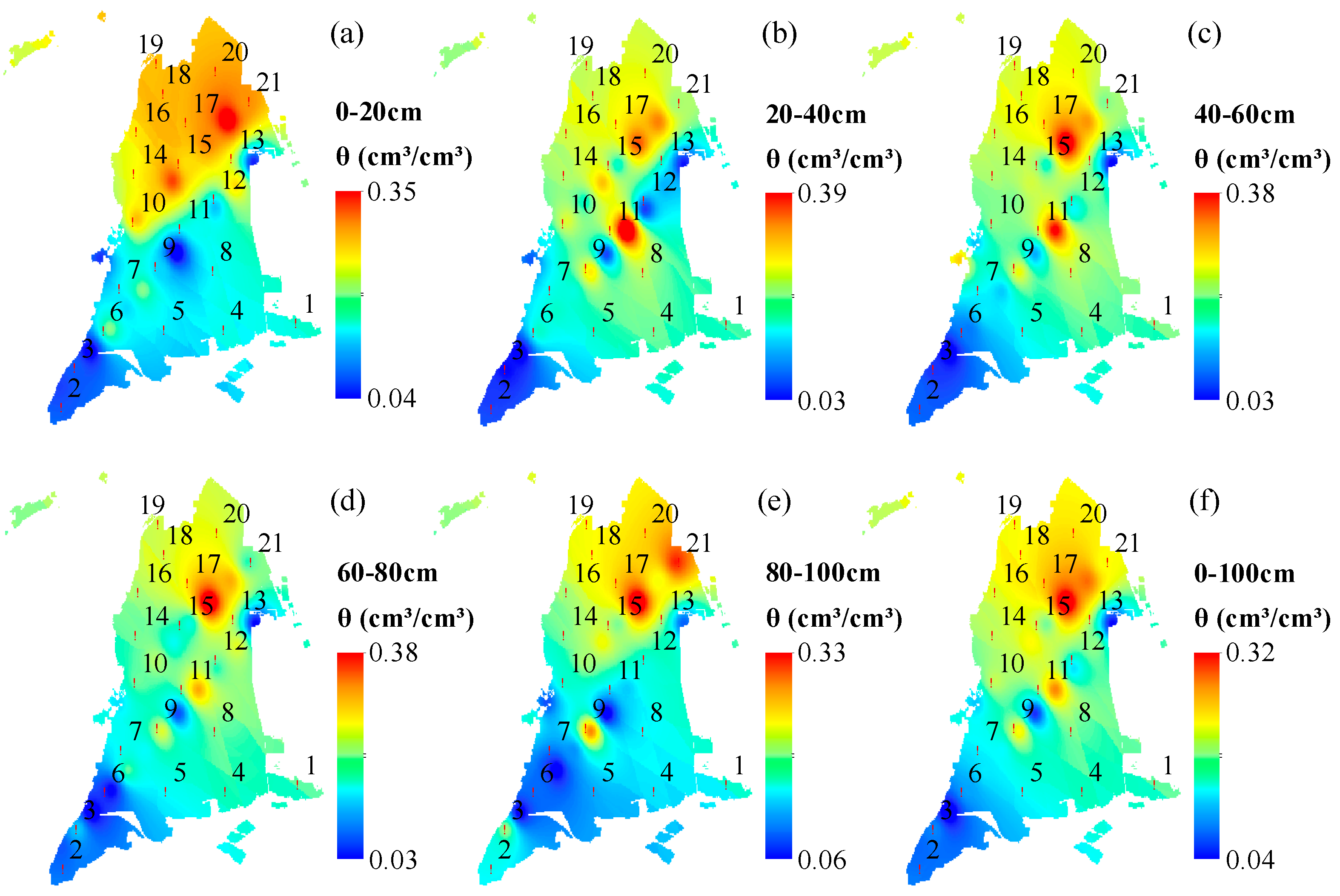
3.1. Spatial Ditribution of the Soils and Sediments Moistures

3.1.1. Regional Distribution of Soil Moisture and the Influence Factors

According to the spatial distribution map of soil moisture measured before the first irrigation in each layer (Figure 4), the soil moisture at depth of 0–100 cm is large in the north and east parts and small in the south and west. Combined with the geographical environment of the oasis (Figure 1b), the Yaoba Oasis, which is located between the Helan Mountain and the Tengger Desert, evidently belongs to the mountain–oasis–desert system (MODS), a basic geographic landscape in arid areas of China [55]. From the ecosystem function, the mountain system provides water resources for the oasis, which serves as a site for agricultural production and social development, while the desert is the vast moisture dissipation region [56]. For the stream link, the MODS is the ordered pattern of upstream, midstream, and downstream [57]. With regard to soil permeability, the hydraulic conductivities are larger in the east than that in the west, as shown in Figure 2. As a result, the vast amounts of mountain torrents seep deep into the aquifers when flowing through the piedmont-sloped alluvial plain and continue to infiltrate along the west edge of the oasis, leaving little replenishment for the soil water in the east. Eight relatively sizable seasonal ditches are distributed in the piedmont alluvial plain of Helan Mountain (Figure 1b). However, the surface runoff formed during the rainstorm season often appears as a flood peak with large flow and short duration. After the rain, this runoff was exhausted by evaporation and leakage [4]. All the aforementioned factors contributed to the identified spatial distribution pattern of soil moisture in the Yaoba Oasis.

3.1.2. Layered Soil Moisture Characteristics

For layered soils, the vertical distribution of the high-water content area in the north is relatively stable within 20–100 cm (Figure 4b–e), while that of the area with low water content in the south-west corner increases with the depth. The distribution characteristics indicate that the soil moisture has significant spatial heterogeneity in the oasis area. This phenomenon may be caused by oasis microclimate [58]. For the surface layer (0–20 cm) (Figure 4a), an area with high soil moisture is observed in the north. Theoretically, the surface soil is the water deficit layer on the condition of the absence of irrigation and precipitation accompanied by strong evaporation in the early stage before the observation. A reasonable explanation for this condition is the condensation of dew from the near-surface air [59]. Zhuang et al. [60] reported that dew is a key source of water for sand-fixing plants in desert oases. Jia et al. [61] stated that dew is a slightly stable water resource to maintain the biodiversity for the arid desert areas. Additional research suggests that dew is a stable and sustainable non-rainfall water supply to agriculture [62,63,64]. In conclusion, the spatial soil moisture was mainly affected by the surrounding geography (mountain and desert), regional permeability, stream link direction, runoff features, microclimate, and dewfalls.

3.2. Vertical Distribution of Soil Moisture at Individual Points

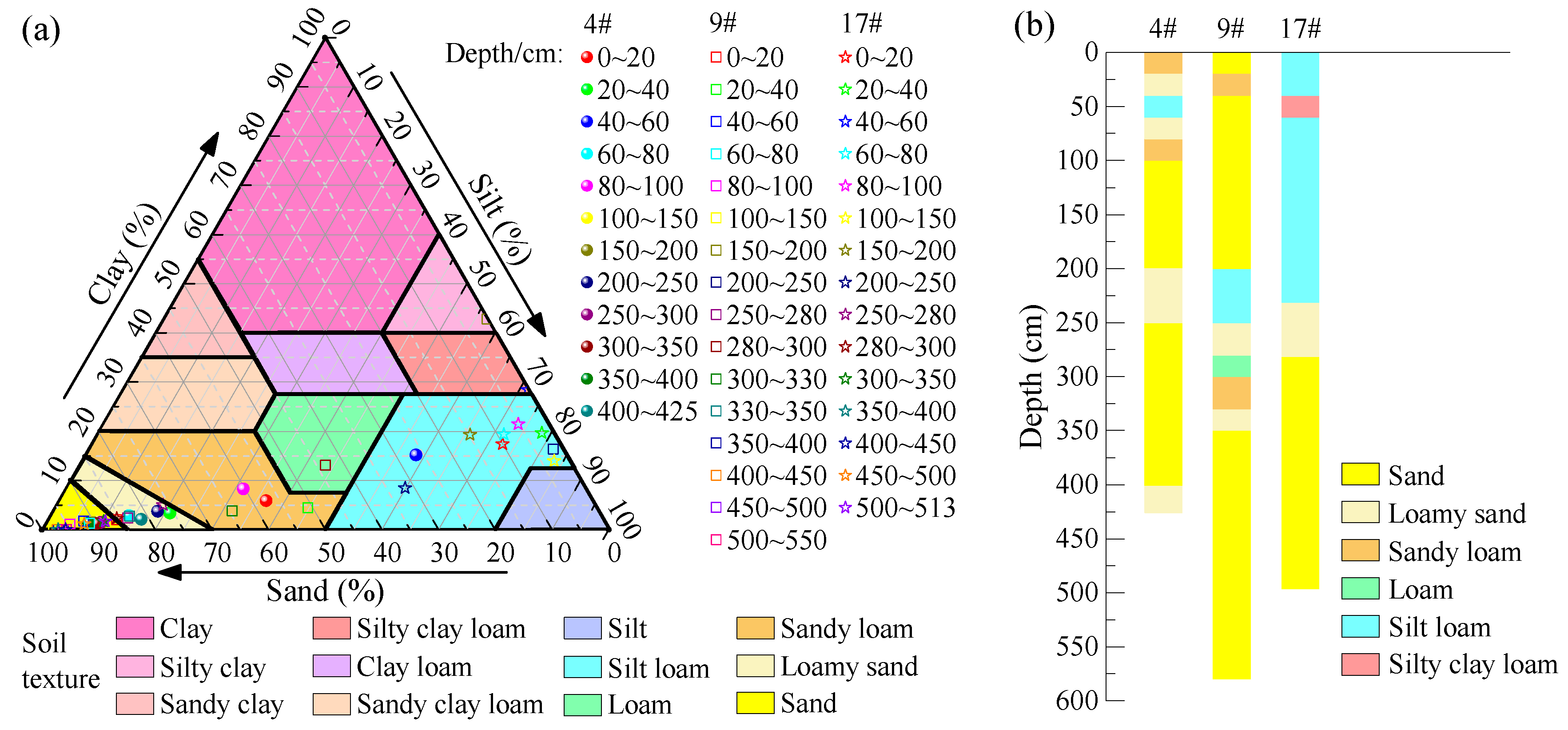
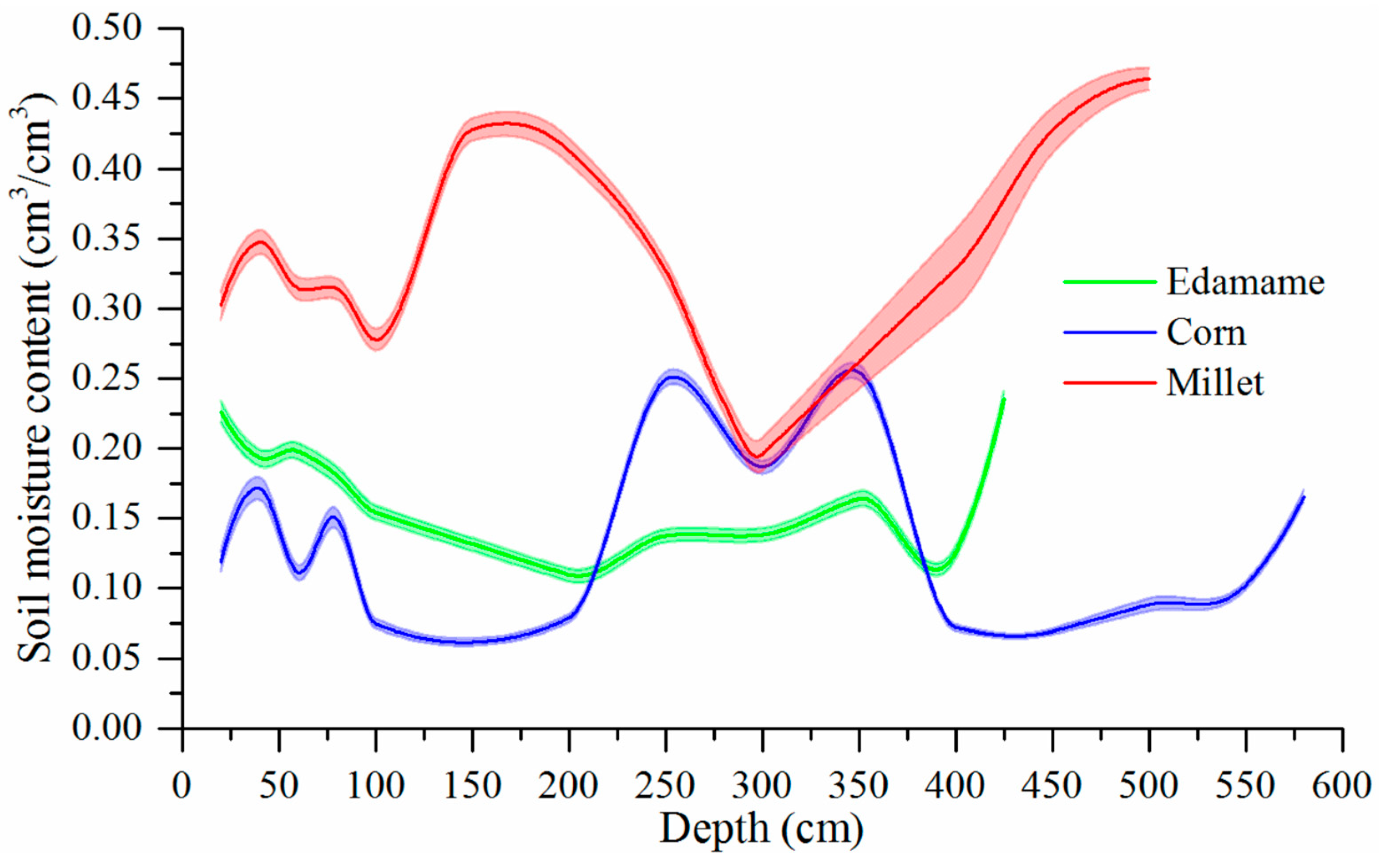
3.2.1. Influence of Soil Texture on the Soil Moisture

Figure 5 shows that the water content on the soil profile before the two irrigations demonstrates an uneven “S” type distribution with the change of the buried depth, and no direct linear relationship is observed between the moisture content and the buried depth.
Combined with the soil texture in Figure 3, the vertical distribution of soil moistures was found to be mainly influenced by soil textures along the profile [65]. The analysis of the turning points in Figure 5 shows that at point 4 (Figure 5a), the soil at a depth of 200 cm is sand, while the upper and lower layers are all loamy soil. The sand layer has low water storage capacity, resulting in low soil content. Similarly, the soil at a depth of 400 cm is sand, while the upper and lower layers are all sandy loam. The sand layer at this depth has low water storage capacity, resulting in low soil content. At point 9 (Figure 5b), the soil at 60, 300, and 350 cm is different from that at the upper and lower layers. At point 17 (Figure 5c), the soil at 300–400 cm is different from that at the upper and lower layers. When the groundwater buried depth is large (more than 10 m) [46], the vertical distribution of soil moisture evidently has no relationship with the depth of the soil layer but is closely related to the soil texture [66].

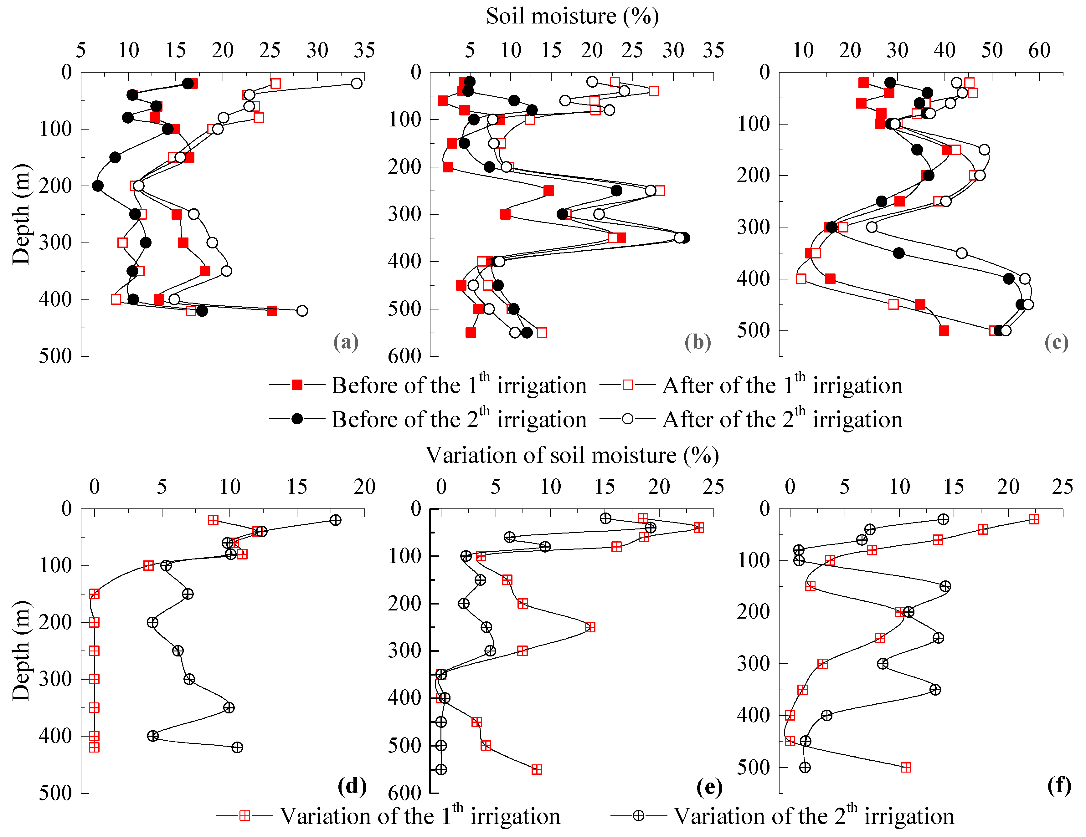
3.2.2. Variation Characteristics of Soil Moisture Affected by Irrigation Activities

At point 4 (Figure 5a,d), the soil layers within 1.5 m of the buried depth are quickly replenished in 6 h after the first irrigation, and the soil moisture content ranges from 4% to 12.08%, increasing to 0.27–1.15 times the original moisture content. The soil layers in the thickness of 4.25 m from top to bottom are replenished in 8 h after the second irrigation, and the soil moisture content ranges from 4.42% to 17.78%, increasing to 0.37–1.19 times the original content.
At point 9 (Figure 5b,e), except for the soil layers of 350–400 cm, the soil moisture content of each layer within 5.8 m is replenished in 24 h after the first irrigation, and the soil moisture contents are changed between 3.29% and 23.64%, of which the soil moisture content at 60 cm increases to 10.8 times. The soil layers within 3 m thickness from the surface are replenished in 24 h after the second irrigation, and the soil moisture contents change between 2.08% and 19.22%, of which the soil moisture content at 40 cm increases to 4 times.
At point 17 (Figure 5c,f), except for 450 cm, the other soil layers are replenished in 18 h after the first irrigation, the growth range is between 2.98–22.38%, and the water content at 20 cm increases by nearly two times. The soil layers within 5 m are replenished in 24 h after the second irrigation, and the soil moisture content generally increases by 3.36% to 14.24%.
The preceding analyses show that the recharge effects of irrigation on soil moisture are significant, but the recharge depth and degree of each test point are different. The maximum observation recharge depth at point 4 is 4.25 m, the soil moisture content is between 3.1% and 27.44%, and the highest is more than four times before irrigation. Meanwhile, the maximum observation recharge depth at point 9 is 5.8 m, soil water content variation is between 2.08% and 23.64%, and the highest is 10.8 times before the irrigation. The maximum observation recharge depth at point 17 is 5 m, and the soil moisture content variation is between 2.57% and 22.38%.

3.3. Influence Factors of Vertical Soil Moisture along Profiles

During the monitoring period, the soil moisture of the three different crop types was completely different (Figure 6). Overall, the mean soil moisture presents the following order: corn > edamame > millet. Regarding the fluctuation characteristics of the moisture content, the edamame slightly changed while those for corn and millet considerably varied along the profiles. The reasons for such results are mainly reflected in three aspects: soil moisture requirement, soil textures, and preferential flow.

3.3.1. Influence of Soil Moisture Requirement

The three crops have different water requirements following the order: corn > edamame > millet [67]. The evapotranspiration of corn is evidently much larger than that of millet. Consequently, when the water requirement of the crop is large, the soil moisture content at the observation point under the same water supply conditions is small.

3.3.2. Influence of the Layered Soil Textures

The soil textures vary with the soil profiles. For corn and millet, at the depth of 0–100 and 250–350 cm, the fluctuation trends are similar but that in the depth of 100–250 and >350 cm appear to be the opposite. For corn, the moisture is symmetrically distributed from 100 cm to 500 cm because the soil texture is also nearly symmetrically distributed within the corresponding depths. The textures of the high water content range are mainly sandy loam, silt loam, loamy sand and loam, and of the valleys on both sides of the peak are mainly sand. Combined with the soil texture shown in Figure 3, the varying characteristics of soil moisture of the three points agree with the vertical distribution of soil texture, which is consistent with the research of Wang et al. [66].

3.3.3. Influence of Preferential Flow

The soil moisture curves of millet and edamame show a moisture valley in the vicinity of 300 and 400 cm, respectively, but present a sudden increase at large depths. A sharp rise of soil moisture at the depth of 300–400 cm is unusual. Evidently, the irrigation water cannot replenish such depths through uniform piston flow [40,68]. This phenomenon is reasonably due to the effect of preferential flow [34,35,46]. The aforementioned layers are developed with macropores and pipes formed by bioactivities, which provide dominant infiltration channels for the water to rapidly penetrate through the soil matrix [43,44], resulting in a rapid decline of soil moisture in the top layer and a sharp increase in the bottom layers. The preceding analysis indicates that moisture does not linearly change with depth due to the existence of preferential flow under the irrigation condition and the non-uniform texture profile. This phenomenon is common in arid oases [35]. Therefore, preferential flow, which is the main recharge form for deep ground water, is important for the sustainability of crop growth.

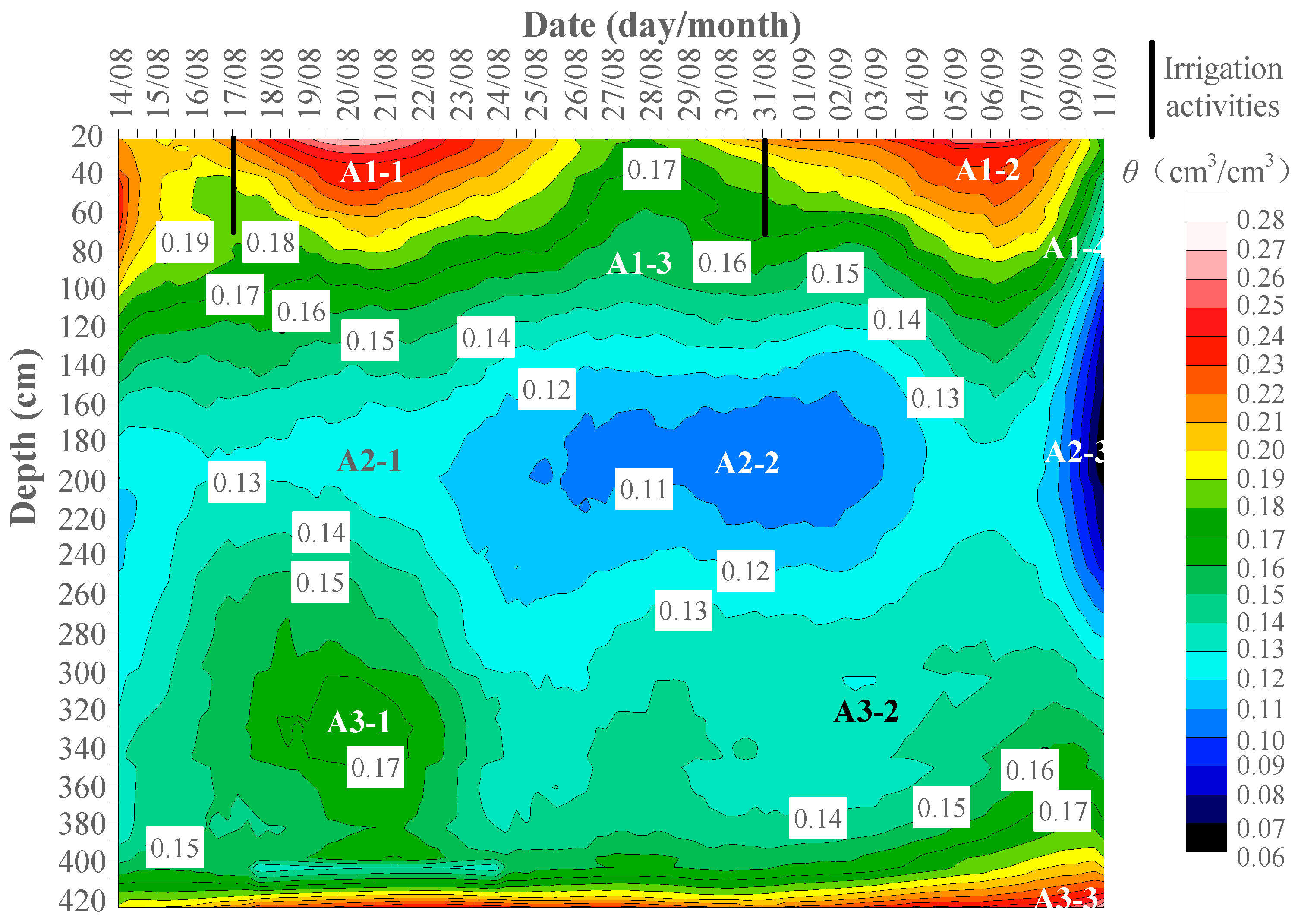
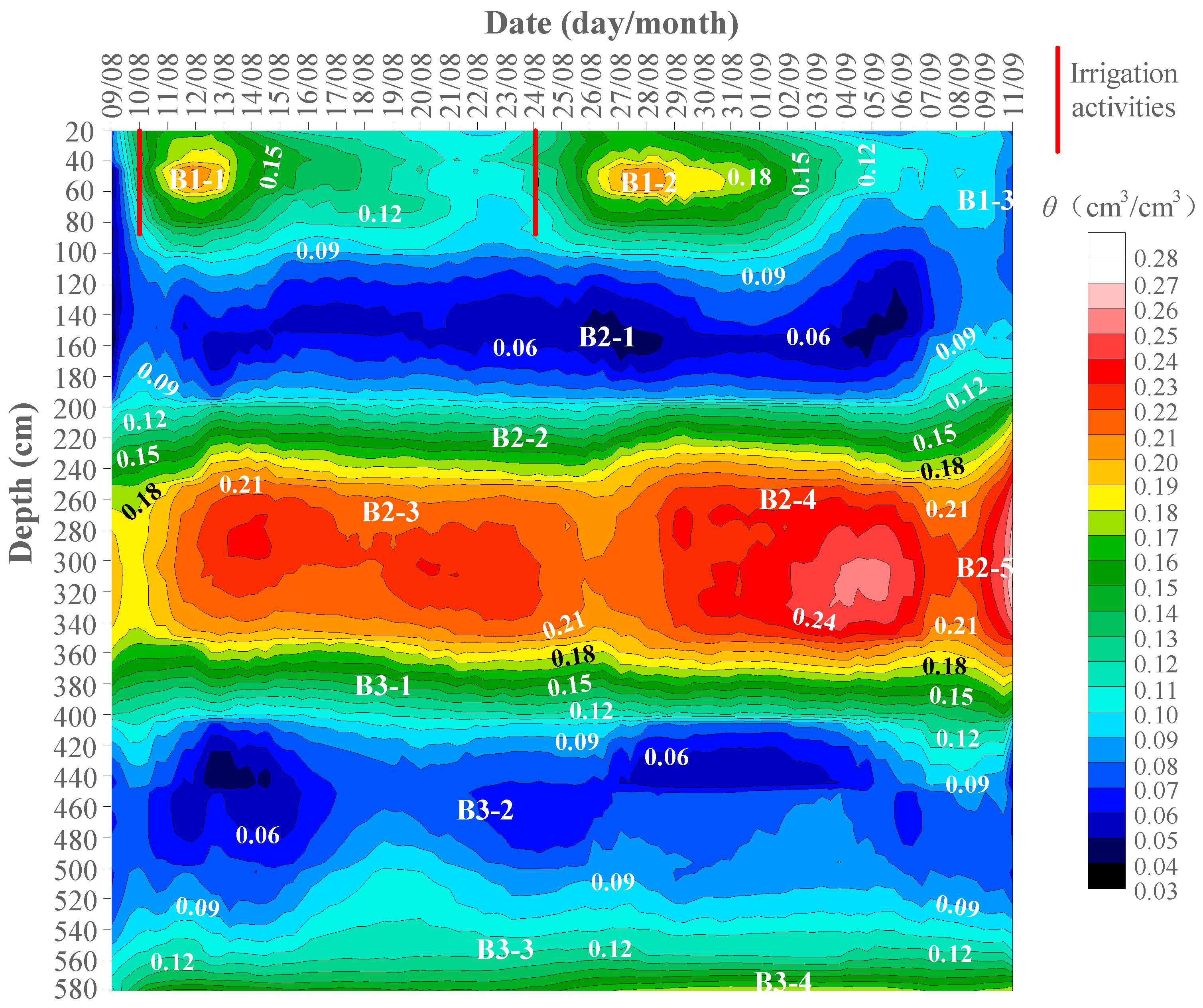
3.4. Spatial–Temporal Variation of the Layered Soils and Sediments Moistures

The soil moisture variation isogram with respect to depth and time was mapped (Figure 7, Figure 8 and Figure 9) using Surfer 11 according to the regression equations obtained through LPRI. This section individually analyzes the characteristics of each depth range.

3.4.1. Variation of Soil Moisture Content with Time within 1 m

The shallow soils within 1 m are susceptible to temperature, precipitation, water channel leakage, irrigation activities, and other factors, all of which result in considerable water content fluctuation. Among all the factors, the effect of irrigation is the most evident. Figure 7, Figure 8 and Figure 9 show that the soil moisture contents within 1 m in the observed pores are quickly replenished after irrigation, and the maximum moisture content is reached after 6 to 24 h. At points 4 (Figure 7) and 9 (Figure 8), the soil moisture content of each layer within 1 m drastically increases after irrigations, as demonstrated by the soil moisture districts of A1-1, A1-2, B1-1, and B1-2. Point 17 is less able to receive replenishment compared with that of the two other points due to its large initial water content (Figure 9). In addition, considering the large permeability and poor water retention of the surface sand texture, the soil moisture content is quickly replenished after irrigation and then rapidly infiltrates into the deep layer. As a result, the soil moisture content of point 17 does not increase, as shown by the districts of C1-1–C1-3. However, this point maintains a high moisture content (bigger than 0.20 cm3/cm3) during the entire observation period.
At point 4 (Figure 7), from left to right (start to end of irrigation), whether it is the first or the second irrigation, the colors follow the order of green–yellow–orange–red–orange–yellow–green, indicating that the moisture goes through the stages of low–increased–stable–low consumption (A1-1 or A1-2). Eventually, soil moisture may enter into the state of water scarcity, in which the color of the contour zone will become cyan or even blue (A1-4), and the isolines will be compacted. The occurrence of this phenomenon indicates the entrance into the rapid consumption period of soil moisture and the disappearance of the water replenishment effect of the previous irrigation. Compared with the moisture effect duration of the first irrigation, the irrigation period at this point should be maintained at intervals of 13 to 15 days. Similar conclusions can also be drawn from points 9 and 17 (Figure 8 and Figure 9, respectively).

3.4.2. Variation of Soil Water Content with Time within 1–3 m

Figure 7 illustrates that at point 4, part of the water infiltrated downward through the dominant channel. The soil moisture content at 1–3 m immediately considerably fluctuates. The soil in this section has good water permeability and poor water holding capacity because it is dominated by sand and sandy loam. When receiving the rapid replenishment of water from the surface, the excess water is continuously transported downward and emerges in a water deficit region. At the depth of 100–150 cm, the contour zone remains green (A1-3); at 150–250 cm, the contour zone changes to blue (A2-2); at 250–300 cm, the color recovers to green (A3-1). The aforementioned changes in color are strong evidence of preferential flow. Notably, at point 9 (Figure 8), the soil moisture within 1–2 m remains relatively stable and maintains a low content of soil moisture (B2-1) while that at 2–3 m fluctuates heavily after the irrigation (B2-2). This special phenomenon implies the presence of evident preferential flow during irrigation. At point 17 (Figure 9), the soil moisture content slightly increases (C2-2 and C2-3) compared with the surface soil fluctuation (C1-1–C1-3) after irrigation. On the 11th day after the first irrigation, the soil moisture content considerably increases, and the fluctuation is evident. This fluctuation might be caused by the preferential flow and upper penetration. The growth and fluctuation continue until the second irrigation. The slowing down of this fluctuation has not been observed yet due to the short observation time.

3.4.3. Variation of Soil Moisture Content with Time below 3 m

It can be seen from Figure 7 that the soil moisture content of 3.0–4.25 m (A3-1–A3-4) at the 4th point after two irrigations continually keeps with a large fluctuation. The 9th point (Figure 8) maintains relatively stable except for the depth at 330 cm, 350 cm and 580 cm. As with point 17 (Figure 9), the soil moisture content deeper than 3 m shows a substantial increase on the 13th day after the first irrigation, and this trend is maintained for 6 days. Soon after, a second irrigation activity is carried out, and some irrigation water is quickly replenished through the preferential pathways channel to the depth deeper than 3 m. It results in a continuously high level of soil moisture content until the observation experiment is finished. It is speculated that there may be intermittent large pores in the soil profile, so that part of the soil water quickly enters the deeper soil layer in the form of preferential flow for recharge. It is noted that there is continuous water outflow at the soil layer of 5 m and the water content is kept at 25% to 30%. It is inferred that there exists a thin aquifer in the layer, which forms some local perched water.
In conclusion, in the isograms, with respect to time series, when the color of the contour zone varies, this represents the water activities (e.g., irrigation replenishment or dissipation); when the contours are evenly spaced, the soil moisture is in a stable period. When the contour is dense, the water is quickly replenished or dissipated. In terms of depth, the rapid change of soil moisture color from blue to red in a small depth interval indicates the preferential infiltration phase. The slow variation of color in a large depth interval indicates the piston flow infiltration phase.

3.5. Infiltration Pattern and Stage Characteristics

During the irrigation test, the thickness of the field water was maintained at 5–10 cm. The vertical infiltration rate of soil moisture is always larger than the horizontal due to the force of the pressure head [46]. Therefore, the irrigation water is mostly consumed in the vertical infiltration, and the horizontal and lateral seepage is negligible. According to the characteristics of soil moisture content variation during the entire observation period, the infiltration process can be divided into the following three stages according to the main infiltration manners:
Stage 1: Infiltration with preferential flow. The soil moisture content of the layers within 1 m had a significant increase without lags in 6 to 24 h after the first irrigation. This finding indicates that the recharge of the irrigation water quickly arrived at certain layers through the dominant channels, such as wormholes, root holes, and other pathways, to facilitate preferential flow [34,43]. The soil remained in a high moisture state in the next 5 to 7 days due to preferential flow.
Stage 2: Infiltration with piston flow. The soil moisture content changes slowly with time. A certain soil layer received the upper water supply and simultaneously transported the excess water to the lower layer [68]. Subsequently, the soil moisture content gradually returned to its level before irrigation. During this time, the infiltration was mainly in the form of a piston flow which lasts for approximately 5 to 7 days.
Stage 3: Balance and stable infiltration. Through the two previous stages, the soil moisture content returned to the water state before irrigation for approximately half a month after irrigation. During the period starting from this time node to the next irrigation, the soil moisture entered into a stable phase of self-balancing with slight fluctuations. The duration of this stage is determined by the irrigation regime, which may be long or short.
The infiltration stages generally determine the irrigation regime. At the third stage, the replenishment effect of irrigation almost disappears. Therefore, the next irrigation may be conducted at this stage. In conclusion, the irrigation cycle in this study should be maintained for approximately half a month to ensure the normal growth of crops.

3.6. Limitations and Future Research

This paper demonstrates a few limitations. The observation period of this study only lasts for 1 month, but the high-precision observation is sufficient to reveal the influence of preferential flow on soil moisture change under irrigation conditions. The influence of the preferential flow was only qualitatively analyzed using the isogram. Research via dye tracing, isotope technique, computed tomography, or ground penetrating radar should be conducted long term to quantitatively investigate the preferential flow and assess the influence degree on the soil moisture utilization in the entire oasis. In addition, the dew should be thoroughly studied along with the affected factors, formation conditions, and utilization rate. Optimal planting structure should be designed according to crop water requirement, and underground reservoir should be constructed to collect and store the flood and match the flood intercepting along the eastern edge of the oasis. Furthermore, the appropriate irrigation regimes and water-saving irrigation systems should be set up in the future to fully utilize the various forms of water resources and provide a scientific basis for the sustainable development of oasis agriculture.

4. Conclusions

The main objective of this study is to reveal the influencing factors of the spatial–temporal variation of layered soils and sediments moistures and infiltration characteristics under irrigation in Yaoba Oasis. On the basis of the double-ring infiltration test of the hydraulic conductivities, the high-precision monitoring of the soil moisture using the neutron moisture meter, and the accurate calibration of the soil moisture, a permeability map was produced using MRBF; spatial soil moisture distribution maps were interpolated using IDW; and the spatial–temporal isograms of soil moistures with depth and time along profiles were mapped using LPRI.
Through detailed analyses, the influencing factors of the (1) regional spatial soil moistures were ascertained with the mountain and desert, permeability, stream link direction, runoff features, microclimate, and dewfalls; (2) spatial layered soils and sediments moistures were microclimate and dew condensation; and (3) spatial–temporal variation at point site profiles were soil texture, water requirement, and preferential flow.
The initial soil moisture content profiles before the two irrigations show an uneven “S”-type distribution with a change of the buried depth. No direct linear relationship among the soil depths was found, but a close correlation with soil texture was observed. After irrigation, soil moistures increased significantly by 3.1–27.44% at point 4, 1.57–23.64% at point 9 and 2.57–22.38% at point 17. The maximum increase was 10.8 times the original state. Moreover, the recharging depth was promoted deeply up to 580 cm with the aid of preferential flow.
The spatial–temporal variation of soil moisture under irrigation indicates that the best irrigation frequency should be 15 days per time. In addition, the infiltration process can be divided into the preferential flow, piston flow, and balanced infiltration stages owing to the existence of preferential flow. This result indicates that the LPRI is an exceptional method that can not only show the fluctuation laws of soil moisture in the vertical profiles but can also present the change of soil moisture over time in the entire irrigation period. Consequently, the irrigation regime and effects of preferential flow during irrigation are clearly illustrated.
In summary, this paper clearly identified the main influencing factors affecting the spatial and temporal variability of soil moisture under irrigation conditions. In addition, the infiltration forms of irrigation water were ascertained, the water infiltration stages were divided, and the optimal irrigation period was proposed. In the future, a thorough quantitative study of preferential flow on the temporal stability of soil moisture in Yaoba Oasis will be performed.

Author Contributions

Conceptualisation, X.L. and Y.L.; methodology, X.L.; software, X.L.; validation, X.L. and Y.L.; formal analysis, X.L. and R.Z.; investigation, X.L., R.Z., X.Z. and W.P.; resources, X.L. and X.Z.; data curation, X.L. and R.Z.; writing—original draft preparation, X.L.; writing—review and editing, X.L. and Y.L.; visualisation, X.L.; supervision, Y.L.; project administration, W.F.; funding acquisition, W.F. and W.P.

Funding

This research was funded by the National Natural Science Foundation of China (grant number: 41630634) and the Major Research Project for Creative Group of Guizhou Provincial Department of Education (grant number: QJH-KY [2016]054 and QJH-KY [2016]055).

Conflicts of Interest

The authors declare no conflict of interest.

Appendix A

Table A1. Soil physical properties of 4#, 9# and 17# test points.
DepthSoil Particle Composition (%)Soil TextureBulk Density (g/cm3)Initial Water Content (cm3/cm3)
SandClaySilt
4#
0–2057.45.936.7Sandy loam1.610.23
20–4075.73.321.0Loamy sand1.580.18
40–6026.415.158.5Silt loam1.510.21
60–8083.22.814.0Loamy sand1.580.20
80–10060.38.231.5Sandy loam1.610.16
100–20089.51.68.9Sand1.520.12
200–25077.73.718.6Loamy sand1.580.13
250–40089.91.38.8Sand1.520.16
400–42581.42.116.5Loamy sand1.580.22
9#
0–2085.72.012.3Sand1.490.12
20–4050.94.344.8Sandy loam1.610.18
40–20093.71.05.3Sand1.520.10
200–2501.616.382.1Silt loam1.510.19
250–28083.62.414.0Loamy sand1.580.26
280–30043.313.143.6Loam1.500.13
300–35064.53.831.7Sandy loam1.610.25
350–58096.50.03.5Sand1.520.08
17#
0–406.018.575.5Silt loam1.510.34
40–600.028.471.6Silt clay loam1.560.33
60–25012.616.570.9Silt loam1.510.37
250–30080.83.615.6Loamy sand1.580.22
300–50092.20.96.9Sand1.520.38

References

  1. Han, D. Knowledge of a few issues on oasis. J. Arid Land Resour. Environ. 1995, 9, 13–31. (In Chinese) [Google Scholar] [CrossRef]
  2. Postel, S. The Last Oasis: Facing Water Scarcity; Routledge: London, UK, 2014. [Google Scholar] [CrossRef]
  3. Chen, Y.; Li, Z.; Li, W.; Deng, H.; Shen, Y. Water and ecological security: Dealing with hydroclimatic challenges at the heart of China’s Silk Road. Environ. Earth Sci. 2016, 75, 881. [Google Scholar] [CrossRef]
  4. Zhang, M.; Luo, G.; Hamdi, R.; Qiu, Y.; Wang, X.; Maeyer, P.D.; Kurban, A. Numerical simulations of the impacts of mountain on oasis effects in arid Central Asia. Atmosphere 2017, 8, 212. [Google Scholar] [CrossRef]
  5. Li, X.; Yang, K.; Zhou, Y. Progress in the study of oasis-desert interactions. Agric. For. Meteorol. 2016, 230–231, 1–7. [Google Scholar] [CrossRef]
  6. Zhang, Q.; Xu, H.; Li, Y.; Fan, Z.; Zhang, P.; Yu, P.; Ling, H. Oasis evolution and water resource utilization of a typical area in the inland river basin of an arid area: A case study of the Manas River valley. Environ. Earth Sci. 2012, 66, 683–692. [Google Scholar] [CrossRef]
  7. Li, H.; Lu, Y.; Zheng, C.; Yang, M.; Li, S. Groundwater level prediction for the arid oasis of Northwest China based on the artificial bee colony algorithm and a back-propagation neural network with double hidden layers. Water 2019, 11, 860. [Google Scholar] [CrossRef]
  8. Song, X.; Zhang, G.; Liu, F.; Decheng, L.; Yuguo, Z.; Jinling, Y. Modeling spatio–temporal distribution of soil moisture by deep learning-based cellular automata model. J. Arid Land 2016, 8, 734–748. [Google Scholar] [CrossRef]
  9. Chen, L.; Feng, Q. Geostatistical analysis of temporal and spatial variations in groundwater levels and quality in the Minqin oasis, Northwest China. Environ. Earth Sci. 2013, 70, 1367–1378. [Google Scholar] [CrossRef]
  10. Yao, L.; Huo, Z.; Feng, S.; Mao, X.; Kang, S.; Jin, C.; Xu, J.; Steenhuis, T.S. Evaluation of spatial interpolation methods for groundwater level in an arid inland oasis, northwest China. Environ. Earth Sci. 2014, 71, 1911–1924. [Google Scholar] [CrossRef]
  11. Zhang, X.; Zhang, L.; He, C.; Li, J.; Jiang, Y.; Ma, L. Quantifying the impacts of land use/land cover change on groundwater depletion in Northwestern China—A case study of the Dunhuang oasis. Agric. Water Manag. 2014, 146, 270–279. [Google Scholar] [CrossRef]
  12. Wang, G.; Zhao, W. The spatio–temporal variability of groundwater depth in a typical desert-oasis ecotone. J. Earth Syst. Sci. 2015, 124, 799–806. [Google Scholar] [CrossRef]
  13. Wang, J.; Gao, Y.; Wang, S. Land use/cover change impacts on water table change over 25 years in a desert-oasis transition zone of the Heihe River Basin, China. Water 2016, 8, 11. [Google Scholar] [CrossRef]
  14. Gu, F.; Zhang, Y.D.; Chu, Y.; Shi, Q.D.; Pan, X. Primary analysis on groundwater, soil moisture and salinity in Fukang oasis of Southern Junggar Basin. Chin. Geogr. Sci. 2002, 12, 333–338. [Google Scholar] [CrossRef]
  15. Cui, G.; Lu, Y.; Zheng, C.; Liu, Z.; Sai, J. Relationship between soil salinization and groundwater hydration in Yaoba Oasis, Northwest China. Water 2019, 11, 175. [Google Scholar] [CrossRef]
  16. Ma, L.; Ma, F.; Li, J.; Gu, Q.; Yang, S.; Wu, D.; Feng, J.; Ding, J. Characterizing and modeling regional-scale variations in soil salinity in the arid oasis of Tarim Basin, China. Geoderma 2017, 305, 1–11. [Google Scholar] [CrossRef]
  17. Qin, S.; Gao, G.; Fu, B.; Lü, Y. Soil water content variations and hydrological relations of the cropland-treebelt-desert land use pattern in an oasis-desert ecotone of the Heihe River Basin, China. Catena 2014, 123, 52–61. [Google Scholar] [CrossRef]
  18. Zucco, G.; Brocca, L.; Moramarco, T.; Morbidelli, R. Influence of land use on soil moisture spatial–temporal variability and monitoring. J. Hydrol. 2014, 516, 193–199. [Google Scholar] [CrossRef]
  19. Zhang, Y.; Xiao, Q.; Huang, M. Temporal stability analysis identifies soil water relations under different land use types in an oasis agroforestry ecosystem. Geoderma 2016, 271, 150–160. [Google Scholar] [CrossRef]
  20. Zhang, S.; Shao, M. Temporal stability of soil moisture in an oasis of northwestern China. Hydrol. Process. 2017, 31, 2725–2736. [Google Scholar] [CrossRef]
  21. Zhang, P.; Shao, M.A. Temporal stability of surface soil moisture in a desert area of northwestern China. J. Hydrol. 2013, 505, 91–101. [Google Scholar] [CrossRef]
  22. Pan, Y.X.; Wang, X.P.; Zhang, Y.F.; Hu, R. Spatio-temporal variability of root zone soil moisture in artificially revegetated and natural ecosystems at an arid desert area, NW China. Ecol. Eng. 2015, 79, 100–112. [Google Scholar] [CrossRef]
  23. Liu, B.; Zhao, W.; Zeng, F. Statistical analysis of the temporal stability of soil moisture in three desert regions of northwestern China. Environ. Earth Sci. 2013, 70, 2249–2262. [Google Scholar] [CrossRef]
  24. Wang, S.; Guo, D.; Fan, J.; Wang, Q. Spatiotemporal variability of surface-soil moisture of land uses in the middle reaches of the Heihe River Basin, China. Environ. Earth Sci. 2016, 75, 1203. [Google Scholar] [CrossRef]
  25. Wang, Y.; Yang, J.; Chen, Y.; Wang, A.; Maeyer, P.D. The Spatiotemporal Response of Soil Moisture to Precipitation and Temperature Changes in an Arid Region, China. Remote Sens. 2018, 10, 468. [Google Scholar] [CrossRef]
  26. Zheng, C.; Lu, Y.; Guo, X.; Li, H.; Sai, J.; Liu, X. Application of HYDRUS-1D model for research on irrigation infiltration characteristics in arid oasis of Northwest China. Environ. Earth Sci. 2017, 76. [Google Scholar] [CrossRef]
  27. Starks, P.J.; Heathman, G.C.; Jackson, T.J.; Cosh, M.H. Temporal stability of soil moisture profile. J. Hydrol. 2006, 324, 400–411. [Google Scholar] [CrossRef]
  28. Jia, Y.; Shao, M.; Jia, X. Spatial pattern of soil moisture and its temporal stability within profiles on a loessial slope in northwestern China. J. Hydrol. 2013, 495, 150–161. [Google Scholar] [CrossRef]
  29. Evett, S.R.; Schwartz, R.C.; Tolk, J.A.; Howell, T.A. Soil profile water content determination: Spatiotemporal variability of electromagnetic and neutron probe sensors in access tubes. Vadose Zone J. 2009, 8, 926–941. [Google Scholar] [CrossRef]
  30. Li, X.; Liu, L.; Duan, Z.; Wang, N. Spatio-temporal variability in remotely sensed surface soil moisture and its relationship with precipitation and evapotranspiration during the growing season in the Loess Plateau, China. Environ. Earth Sci. 2014, 71, 1809–1820. [Google Scholar] [CrossRef]
  31. Li, T.; Hao, X.; Kang, S. Spatiotemporal variability of soil moisture as affected by soil properties during irrigation cycles. Soil Sci. Soc. Am. J. 2014, 78, 598. [Google Scholar] [CrossRef]
  32. Zhou, N.; Wang, Z.; Hao, J. Application of regression isogram to dynamic analysis of soil moisture variations with time and space. Trans. Chin. Soc. Agric. Mach. 1997, 31, 112–115. (In Chinese) [Google Scholar]
  33. Cheng, D.; Zhang, P.; Zhao, J.; Liu, J. Temporal and spatial variability of red soil water under different ground covers by regression isogram. J. Irrig. Drain. 2009, 28, 90–94. (In Chinese) [Google Scholar]
  34. Yan, J.; Zhao, W.; Zhang, Y. Characteristics of the preferential flow and its response to irrigation amount in oasis cropland. Chin. J. Appl. Ecol. 2015, 26, 1454–1460. (In Chinese) [Google Scholar] [CrossRef]
  35. Zhang, Y.; Fu, L.; Zhao, W.; Yan, J. A review of researches of preferential flow in desert-oasis region. J. Desert Res. 2017, 37, 1189–1195. (In Chinese) [Google Scholar] [CrossRef]
  36. Hendrickx, J.M.; Flury, M. Uniform and preferential flow mechanisms in the vadose zone. In Conceptual Models of Flow and Transport in the Fractured Vadose Zone; National Research Council, Ed.; National Academy Press: Washington, DC, USA, 2001; pp. 149–187. [Google Scholar]
  37. Ivanov, A.L.; Shein, E.V.; Skvortsova, E.B. Tomography of soil pores: From morphological characteristics to structural–functional assessment of pore space. Eurasian Soil Sci. 2019, 52, 50–57. [Google Scholar] [CrossRef]
  38. Wu, Q.; Zhang, J.; Lin, W.; Wang, G. Appling dyeing tracer to investigate patterns of soil water flow and quantify preferential flow in soil columns. Trans. Chin. Soc. Agric. Eng. 2014, 30, 82–90. (In Chinese) [Google Scholar] [CrossRef]
  39. Shein, E.V.; Devin, B.A. Current problems in the study of colloidal transport in soil. Eurasian Soil Sci. 2007, 40, 399–408. [Google Scholar] [CrossRef]
  40. Sun, L.; Zhang, H.; Cheng, J.; Wang, B.; Lu, X.; Wang, X. Relationship between soil macropore and preferential flow in citrus garden. Bull. Soil Water Conserv. 2012, 32, 75–79. (In Chinese) [Google Scholar] [CrossRef]
  41. Shein, E.V.; Shcheglov, D.I.; Moskvin, V.V. Simulation of water permeability processes in chernozems of the Kamennaya Steppe. Eurasian Soil Sci. 2012, 45, 578–587. [Google Scholar] [CrossRef]
  42. Shein, E.V.; Skvortsova, E.B.; Dembovetskii, A.V.; Abrosimov, K.N.; Il’In, L.I.; Shnyrev, N.A. Pore-size distribution in loamy soils: A comparison between microtomographic and capillarimetric determination methods. Eurasian Soil Sci. 2016, 49, 315–325. [Google Scholar] [CrossRef]
  43. Zhang, Y.; Zhao, W.; Fu, L. Soil macropore characteristics following conversion of native desert soils to irrigated croplands in a desert-oasis ecotone, Northwest China. Soil Tillage Res. 2017, 168, 176–186. [Google Scholar] [CrossRef]
  44. Zhang, Y.; Zhao, W.; He, J.; Fu, L. Soil susceptibility to macropore flow across a desert-oasis ecotone of the Hexi Corridor, Northwest China. Water Resour. Res. 2018, 54, 1281–1294. [Google Scholar] [CrossRef]
  45. Bodhinayake, W.; Si, B.C.; Noborio, K. Determination of hydraulic properties in sloping landscapes from tension and double-ring infiltrometers. Vadose Zone J. 2004, 3, 964–970. [Google Scholar] [CrossRef]
  46. Zhang, R. Study on the Infiltration Law of the Irrigation Water in the Yaoba Oasis; Chang’an University: Xi’an, China, 2016. (In Chinese) [Google Scholar]
  47. Zhijie, L. Analysis on the Utilization Efficiency of Agricultural Water Resources in Yaoba Irrigation Area, Alxa; Inner Mongolia Agricultural University: Hohhot, China, 2015. (In Chinese) [Google Scholar]
  48. Tang, G.; Yang, X. ArcGIS: Spatial Analysis Experiment Tutorial of Geographical Information System, 2nd ed.; Geographic Information Systems Theory and Applications Series; Science Press: Beijing, China, 2012. (In Chinese) [Google Scholar]
  49. Nam, M.-D.; Thanh, T.-C. Numerical solution of Navier–Stokes equations using multiquadric radial basis function networks. Int. J. Numer. Methods Fluids 2001, 37, 65–86. [Google Scholar] [CrossRef]
  50. Chaplot, V.; Darboux, F.; Bourennane, H.; Leguédois, S.; Silvera, N.; Phachomphon, K. Accuracy of interpolation techniques for the derivation of digital elevation models in relation to landform types and data density. Geomorphology 2006, 77, 126–141. [Google Scholar] [CrossRef]
  51. Ashiq, M.W.; Zhao, C.; Ni, J.; Akhtar, M. GIS-based high-resolution spatial interpolation of precipitation in mountain–plain areas of Upper Pakistan for regional climate change impact studies. Theor. Appl. Climatol. 2010, 99, 239–253. [Google Scholar] [CrossRef]
  52. Miller, H.J. Tobler’s first law and spatial analysis. Ann. Assoc. Am. Geogr. 2004, 94, 284–289. [Google Scholar] [CrossRef]
  53. Waters, N. Tobler’s first law of geography. In The International Encyclopedia of Geography; John Wiley & Sons, Ltd.: Hoboken, NJ, USA, 2017. [Google Scholar] [CrossRef]
  54. Li, Y.; Fang, Z.; Wei, Y. Suppressing end effect of EMD based on local polynomial regression. J. Univ. Sci. Technol. China 2014, 44, 786–792. (In Chinese) [Google Scholar] [CrossRef]
  55. Xu, L.; Zhou, H.; Pan, F.; Wu, L.; Tang, Y. Spatial variability of precipitation for mountain-oasis-desert system in the Sangong River Basin. Acta Geogr. Sin. 2016, 71, 731–742. [Google Scholar] [CrossRef]
  56. Wei, H.; Xu, Z.; Liu, H.; Ren, J.; Fan, W.; Lu, N.; Dong, X. Evaluation on dynamic change and interrelations of ecosystem services in a typical mountain-oasis-desert region. Ecol. Indic. 2018, 93, 917–929. [Google Scholar] [CrossRef]
  57. Cai, Y.; Huang, W.; Teng, F.; Wang, B.; Ni, K.; Zheng, C. Spatial variations of river–groundwater interactions from upstream mountain to midstream oasis and downstream desert in Heihe River basin, China. Hydrol. Res. 2016, 47, 501–520. [Google Scholar] [CrossRef]
  58. Xue, J.; Gui, D.; Lei, J.; Sun, H.; Zeng, F.; Mao, D.; Zhang, Z.; Jin, Q.; Liu, Y. Oasis microclimate effects under different weather events in arid or hyper arid regions: A case analysis in southern Taklimakan desert and implication for maintaining oasis sustainability. Theor. Appl. Climatol. 2018, 8, 2567–2579. [Google Scholar] [CrossRef]
  59. Tomaszkiewicz, M.; Najm, M.A.; Beysens, D.; Alameddine, I.; El-Fadel, M. Dew as a sustainable non-conventional water resource: A critical review. Environ. Rev. 2015, 23, 425–442. [Google Scholar] [CrossRef]
  60. Zhuang, Y.; Zhao, W. Dew formation and its variation in Haloxylon ammodendron plantations at the edge of a desert oasis, northwestern China. Agric. Forest Meteorol. 2017, 247, 541–550. [Google Scholar] [CrossRef]
  61. Jia, Z.; Zhao, Z.; Zhang, Q.; Wu, W. Dew yield and its influencing factors at the western edge of Gurbantunggut Desert, China. Water 2019, 11, 733. [Google Scholar] [CrossRef]
  62. Wang, H.; Jia, Z.; Lu, Y.; He, Z.; Wang, Y.; Chen, Y.; Zhi, W. Dew condensation time and frequency in the loess hilly region of Ansai County, northern Shaanxi Province, China. Chin. J. Appl. Ecol. 2017, 28. (In Chinese) [Google Scholar] [CrossRef]
  63. Wang, H.; Jia, Z.; Wang, Z. Dew amount and its inducing factors in the loess hilly region of northern Shaanxi Province, China. Chin. J. Appl. Ecol. 2017, 28, 3703–3710. (In Chinese) [Google Scholar] [CrossRef]
  64. Jia, Z.; Wang, Z.; Wang, H. Characteristics of dew formation in the semi-arid Loess Plateau of Central Shaanxi Province, China. Water 2019, 11, 126. [Google Scholar] [CrossRef]
  65. Wang, Y.; Shao, M.A.; Liu, Z.; Warrington, D.N. Regional spatial pattern of deep soil water content and its influencing factors. Hydrol. Sci. J. 2012, 57, 265–281. [Google Scholar] [CrossRef]
  66. Wang, Y.; Shao, M.A.; Liu, Z. Vertical distribution and influencing factors of soil water content within 21-m profile on the Chinese Loess Plateau. Geoderma 2013, 193–194, 300–310. [Google Scholar] [CrossRef]
  67. Chen, Y.; Guo, G.; Wang, G.; Kang, S.; Luo, H.; Zhang, D. China’s Main Crop Water Demand and Irrigation; China Water & Power Press: Beijing, China, 1995. (In Chinese) [Google Scholar]
  68. Wu, Q.; Liu, C.; Lin, W.; Zhang, M.; Wang, G.; Zhang, F. Quantifying the preferential flow by dye tracer in the North China Plain. J. Earth Sci. 2015, 26, 435–444. [Google Scholar] [CrossRef]
Figure 1. Location map of the study area: (a) location of Yaoba Oasis in Inner Mongolia, China; (b) geographic location, stream links, and terrain (based on digital elevation model) of the Yaoba Oasis; (c) land use map of Yaoba Oasis and the layout of test points.
Water 11 01483 g001
Figure 2. Spatial distribution map of hydraulic conductivities of Yaoba Oasis.
Water 11 01483 g002
Figure 3. Soil texture diagram: (a) triangular diagram of soil texture in depth of test points 4#, 9#, and 17# determined by the US Department of Agriculture (USDA) soil texture classification standard; (b) soil texture histogram of test points 4#, 9# and 17# at each layer
Water 11 01483 g003
Figure 4. Spatial distribution map of mean soil moistures of layered soils and sediments measured before the first irrigation of Yaoba Oasis: (af) represent the mean volumetric moisture (θ: cm3/cm3) within 20–40 cm, 40–60 cm, 60–80 cm, 80–100 cm, and 0–100 cm, respectively.
Water 11 01483 g004
Figure 5. Vertical fluctuation curves of the soil and sediment moistures along profiles: (ac) moisture fluctuation curves before and after the first and second irrigations at points 4, 9, and 17, respectively, in which the moisture measurements after the first and second irrigations in (a) were 6 and 8 h, in (b) were all 24 h, and in (c) were 18 and 24 h, respectively; (df) moisture variation curves influenced by the irrigation activities at points 4, 9, and 17, respectively.
Water 11 01483 g005
Figure 6. Relationship curves between mean soil moisture and depth of edamame, corn, and millet with color-filled error bars in the entire observation period.
Water 11 01483 g006
Figure 7. The soil moisture isogram of time and depth at point 4 with the crop of edamame.
Water 11 01483 g007
Figure 8. The soil moisture isogram of time and depth at point 9 with the crop of corn.
Water 11 01483 g008
Figure 9. The soil moisture isogram of time and depth at point 17 with the crop of millet.
Water 11 01483 g009
Table 1. Piecewise grading formula of the neutron moisture meter of each observing points.
IDCalibration EquationApplication Scope (cm)
4# θ V = 0.000064Cn − 0.1479650.850–80
θ V = 0.000864Cn − 2.9270560.9680–400
9# θ V = 0.000049Cn − 0.1021610.810–150
θ V = 0.000038Cn − 0.0470730.82150–200
θ V = 0.000027Cn − 0.0168610.84200–350
θ V = 0.000016Cn − 0.0148550.81350–550
17# θ V = 0.000036Cn + 0.0084910.950–250
θ V = 0.000070Cn − 0.1899220.90250–513
Note: By cautiously calibrating the measured soil moisture data at each test point, a set of best-fitting data were selected to participate in the follow-up studies to ensure the reliability of the results. The selected points were 4#1, 9#1, and 17#3, which respectively represent the results of points 4, 9, and 17 in the context below.
Table 2. Schedule of soil moisture observation and irrigation tests.
IDCrop TypesObservation PeriodIrrigation Activities
Start DateEnd DateFirst TimeSecond Time
4#edamame14 August 201511 September 201517 August 201531 August 2015
9#corn09 August 201511 September 201510 August 201524 August 2015
17#millet15 August 201511 September 201516 August 20153 September 2015
Table 3. Regression equations of points 4, 9, and 17.
IDRegression EquationR2FSignificance
4# y = 0.2626 0.0026 x 1 0.0011 x 2 + 3.9 × 10 6 x 1 x 2
+ 5.2 × 10 5 x 1 2 + 2.2 × 10 6 x 2 2
0.6364.760.00000
9# y = 0.0867 + 0.0001 x 1 + 0.0003 x 2 1.7 × 10 7 x 1 x 2
1.2 × 10 7 x 1 2 4.1 × 10 7 x 2 2
0.295.580.00005
17# y = 0.4007 0.0003 x 1 0.0004 x 2 1.0 × 10 6 x 1 x 2
+ 4.9 × 10 7 x 1 2 + 1.7 × 10 6 x 2 2
0.5351.420.00000

