Modelling Reservoir Turbidity Using Landsat 8 Satellite Imagery by Gene Expression Programming

Abstract

This study aimed to develop a reliable turbidity model to assess reservoir turbidity based on Landsat-8 satellite imagery. Models were established by multiple linear regression (MLR) and gene-expression programming (GEP) algorithms. Totally 55 and 18 measured turbidity data from Tseng-Wen and Nan-Hwa reservoir paired and screened with satellite imagery. Finally, MLR and GEP were applied to simulated 13 turbid water data for critical turbidity assessment. The coefficient of determination (R²), root mean squared error (RMSE), and relative RMSE (R-RMSE) calculated for model performance evaluation. The result show that, in model development, MLR and GEP shows a similar consequent. However, in model testing, the R², RMSE, and R-RMSE of MLR and GEP are 0.7277 and 0.8278, 0.7248 NTU and 0.5815 NTU, 22.26% and 17.86%, respectively. Accuracy assessment result shows that GEP is more reasonable than MLR, even in critical turbidity situation, GEP is more convincible. In the model performance evaluation, MLR and GEP are normal and good level, in critical turbidity condition, GEP even belongs to outstanding level. These results exhibit GEP denotes rationality and with relatively good applicability for turbidity simulation. From this study, one can conclude that GEP is suitable for turbidity modeling and is accurate enough for reservoir turbidity estimation.

1. Introduction

In Taiwan, public water is primarily supplied by reservoirs. The reservoir turbidity quarterly measured by the Environmental Protection Administration (EPA). Turbidity data was released after a strict quality control process [1]. However, although the data are highly accurate, sampling and analysis are considerably time-consuming and are subject to several financial constraints [2]. Additionally, the regional representation of samples from single-point sampling is observed to be insufficient; the test results are debatable if they are estimated based on the inspection results that are obtained from few stations [3]. Therefore, several scholars have recently used satellite imagery to establish the relationship between turbidity and multispectral data as a remote monitoring manner. Roeflsema et al., highlighted that the estimation performed based on a Landsat 7 satellite image exhibits an area coverage rate of 100% and an accuracy of 58%. Compared with the single-point sampling, which covers only 0.5% of the area and which exhibits 100% accuracy, the coverage rate is considerably increased even though the accuracy is reduced; furthermore, the representativeness of the research area is improved [4]. Robert, E. et al., established a turbidity simulation model using satellite spectral data. The result exhibits a high correlation with the measured turbidity, and the coefficient of determination (R²) is 0.89 [5].

Basically, the turbidity simulation model establishment was based on the quantitative relation between telemetry image and turbidity. Those estimation methods can be divided into linear relation, multiple linear regression (MLR) relation, logarithmic relation, exponential relation, Gordan relation, artificial neural networks, supper vector machine (SVM), random forest (RF), partial least squares (PLS), and principal components regression (PCR) [6,7,8,9,10,11,12,13,14,15,16,17,18,19,20,21,22,23,24,25,26,27,28,29,30,31,32,33,34]. However, the empirical relation and observation method used to test different data with various temporal and spatial backgrounds or different measuring instruments, the results of reservoir turbidity estimation are considerably different from those of the original research area [35]. The accuracy of the simulated turbidity by the empirical equation is also influenced by the algorithms. Chang et al., using the high-resolution spectral image obtained from Formosat-2 satellite imagery have a resolution of 8 m and the SSC data of 53 mud samples, the empirical relation that is established using the stepwise regression method exhibit the R² of 0.84 and the relative-RMSE (R-RMSE) of 31%, however, in the case of data validation and testing, R-RMSE improved to 43%, indicating that the empirical relation between the remote sensing imagery and the water quality observations exhibited a considerable degree of error. Therefore, the rationality and applicability of the integrated assessment for relevant research related to the water quality estimation of remote sensing imagery can be improved if the simulated turbidity accuracy is improved and the difference is reduced [36]. Based on the large-area and high-repetition remote sensing imagery and the measured turbidity, this study would like to provide a simulation algorithm for the one who cannot obtain an ideal result in typical algorithms for reservoir turbidity estimation.

2. Materials and Methods

This study refers to Quang, N. H. et al., adopted the high-resolution multi-spectrum satellite Landsat 8 launched by the United States in 2013 for performing spectral data extraction [37]. The turbidity simulation model was developed and validated base on quarterly turbidity data of the Tseng-Wen reservoir, which were measured by the Taiwan EPA [38]. Furthermore, the model was tested by applying the data collected from Nan-Hwa reservoir to evaluate its applicability. Besides, the deterministic pattern and stochastic pattern were used to develop the turbidity simulation model. Subsequently, the R², RMSE, and R-RMSE were applied for the model simulation accuracy assessment.

2.1. Study Area

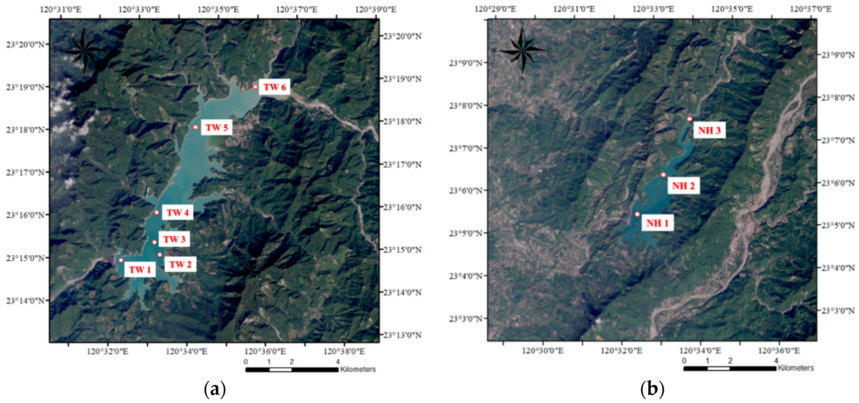
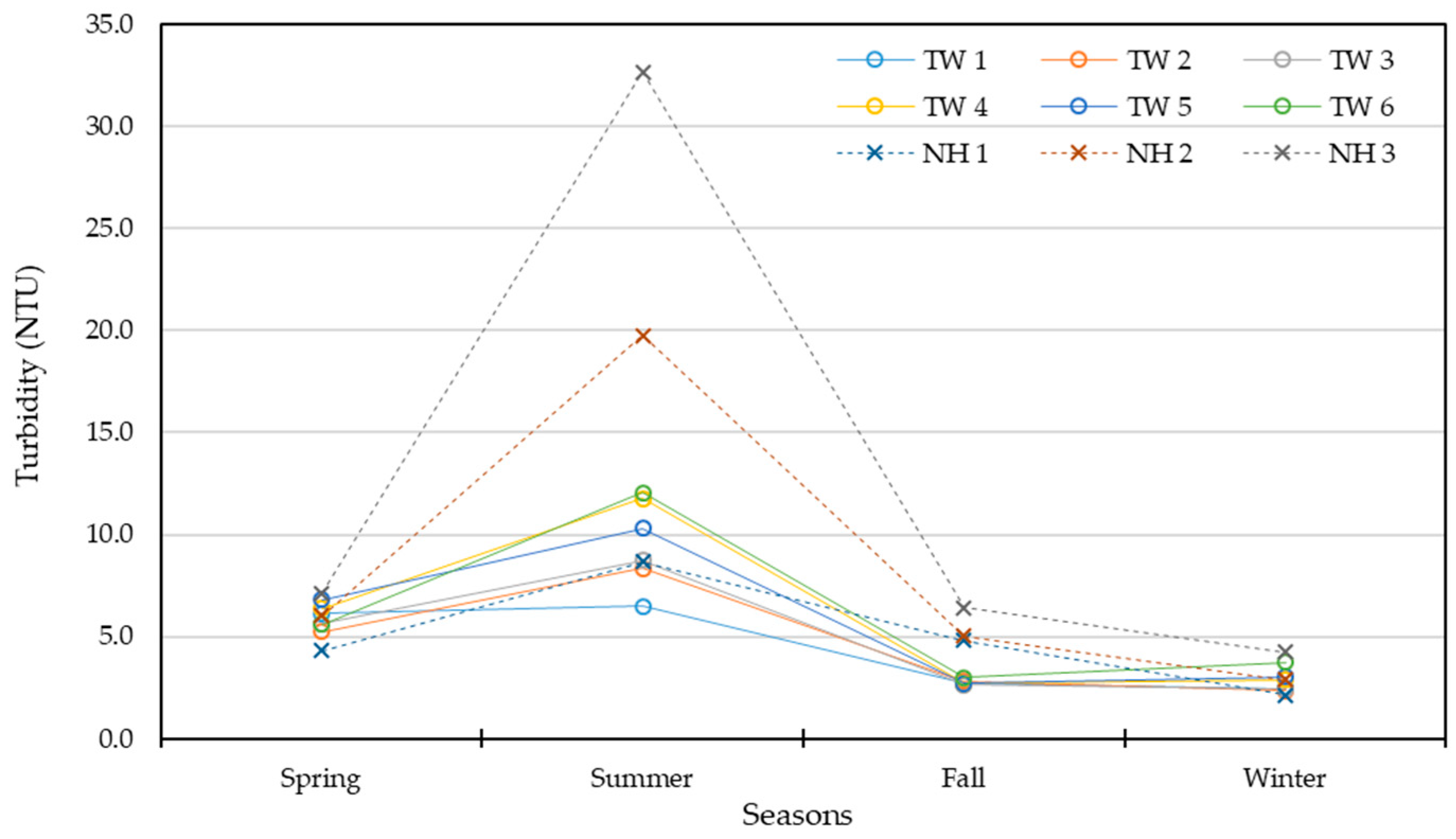
The research area of this study includes the Tseng-Wen reservoir and Nan-Hwa reservoir in Taiwan. The location of turbidity observation stations of the Tseng-Wen and Nan-Hwa reservoirs are depicted in Figure 1. The Tseng-Wen reservoir is located in Da-Pu Township, Chia-Yi County, Taiwan. The reservoir catchment is in Chia-Yi County, the area is 481 Km², the water storage area is 17 Km², and the total water storage capacity is 7.08 × 10⁸ m³. It is the largest reservoir in Taiwan and supplies around 3.988 million tons per day for the public, industrial, and agricultural water supply, which are considered to be the hub of South Taiwan’s livelihood and economy. The turbidity stations of the Tseng-Wen reservoir have been used since 1993 and are named from TW 1 to TW 6. The Nan-Hwa reservoir is located in Nan-Hwa District, Tainan City, Taiwan. The reservoir catchment almost 90% in Tainan City, the area is 108.3 km², and the water storage area is 5.3 km². The water storage capacity is 1.58 × 10⁸ m³. The only target is to supply public water around 0.8 million tons per day. In Nan-Hwa reservoir, three turbidity stations which are named from NH 1 to NH 3, have been operating since 1994. Seasonal turbidity variation (from 2013 to 2018) of Tseng-Wen and Nan-Hwa reservoirs are illustrated in Figure 2, yearly turbidity data of two reservoirs are shown in

Table 1. Yearly turbidity data of Tseng-Wen and Nan-Hwa reservoir.

Season	Station	2013	2014	2015	2016	2017	2018	Avg.
Spring (January to March)	TW 1	13.0	3.4	4.0	4.7	3.4	8.4	6.1
	TW 2	6.7	3.3	5.3	3.8	3.7	8.6	5.2
	TW 3	7.5	4.0	4.2	3.9	3.5	10.7	5.6
	TW 4	8.7	4.6	3.5	3.9	3.7	14.0	6.4
	TW 5	9.2	8.6	4.7	3.8	4.7	10.0	6.8
	TW 6	-	-	6.8	5.1	4.9	-	5.6
	NH 1	4.1	3.7	4.3	5.7	4.0	4.0	4.3
	NH 2	5.8	7.8	6.1	4.8	6.6	5.1	6.0
	NH 3	6.2	11.0	6.3	6.5	-	5.6	7.1
Summer (April to June)	TW 1	3.6	8.1	2.6	2.1	7.6	15.0	6.5
	TW 2	5.5	12.0	2.8	1.7	7.9	20.1	8.3
	TW 3	9.8	8.3	3.8	2.2	9.3	19.1	8.8
	TW 4	12.0	26.0	6.4	2.2	13.0	11.0	11.8
	TW 5	-	-	-	2.6	18.0	-	10.3
	TW 6	-	-	-	3.1	21.0	-	12.1
	NH 1	4.1	16.0	13.0	2.3	7.3	9.2	8.7
	NH 2	3.7	60.0	-	5.8	8.3	21.0	19.8
	NH 3	5.9	85.0	-	9.7	30.0	-	32.7
Fall (July to September)	TW 1	2.7	1.8	2.3	1.6	3.5	4.3	2.7
	TW 2	2.6	2.1	2.0	1.9	3.7	4.7	2.8
	TW 3	2.6	2.0	2.2	1.7	3.4	4.0	2.6
	TW 4	2.9	2.1	1.7	1.6	3.3	4.7	2.7
	TW 5	3.1	2.4	1.4	1.5	3.5	4.4	2.7
	TW 6	-	2.7	2.8	1.9	3.1	4.5	3.0
	NH 1	2.6	2.2	5.6	2.4	3.6	12.5	4.8
	NH 2	3.1	2.8	8.1	2.7	4.8	8.6	5.0
	NH 3	4.9	4.7	7.7	3.4	6.3	11.5	6.4
Winter (October to December)	TW 1	2.6	2.0	1.9	2.5	3.5	2.2	2.5
	TW 2	2.6	1.0	2.0	2.5	3.8	2.2	2.3
	TW 3	2.5	1.3	2.5	2.3	3.4	2.6	2.4
	TW 4	3.7	1.2	3.5	2.6	4.2	2.1	2.9
	TW 5	2.2	2.1	2.3	2.0	5.9	3.6	3.0
	TW 6	2.8	2.6	3.5	2.8	7.8	3.0	3.8
	NH 1	1.4	1.6	1.5	3.1	2.7	2.5	2.1
	NH 2	2.0	2.6	2.2	3.6	3.7	3.3	2.9
	NH 3	3.1	4.1	2.7	5.4	4.6	5.6	4.3

.

The in-situ turbidity measure frequency in Tsing-Wen and Nan-Hwa reservoirs are approximately once per season; however, the observation date and depth of each station are not identical. Therefore, in this study, turbidity data were selected with a water depth of ~1 m to establish the turbidity simulation model.

2.2. Data Collection

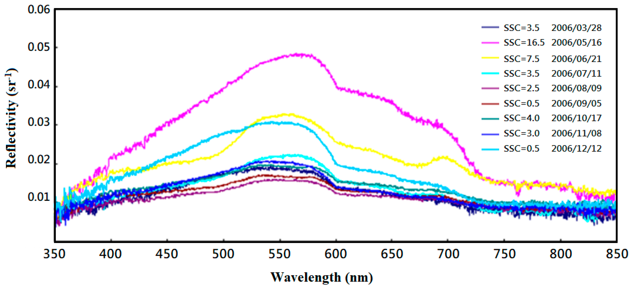
The satellite imagery used in this study were obtained from the Landsat 8 satellite. Considering of the Tseng-Wen reservoir in-situ sediment spectrum data near to the turbidity monitoring station TW 4 obtained by Hsieh, M. L., the wavelength ranging from 350 to 1000 nm, the central reflectance wavelength is around 450 nm to 700 nm as shown in Figure 3 [34]. In addition, according to Doxaran, D. et al., Ma, R. and J, Dai, and Zhou, W. et al., a reasonable spectrum wavelength of turbidity simulation model should deliberate the infrared light spectrum [8,39,40]. Thus, in this study, regard of those previous studies and the spectral wavelength (bands) of Landsat 8, band 2 (450 nm to 510 nm, blue), band 3 (530 nm to 590 nm, green), band 4 (640 nm to 670 nm, red), and band 5 (850 nm to 880 nm) as the model inputs to establish the model.

After selecting the inputs, the observed turbidity data that has to match before and after one day that the satellite passes. Hence, those matched satellite imagery and performing image screening, removing the image of the study area that is covered by the cloud or its shadow, and surface exposure area. The spectral radiation value was converted into the water reflection value according to Robert, E. et al. [5]. Subsequently, the spectral data in the turbidity sampling point was extracted, combined with turbidity data for simulation model development.

2.3. Turbidity Simulation Model Development

Reservoir turbidity simulation model could be developed using the quantitative relation between the acquired satellite spectral data and the measured turbidity data. The traditional model development method—MLR algorithm and the GEP algorithm that has been selected to develop the turbidity simulation model.

2.3.1. Multiple Linear Regression (MLR) Model

The model for estimating the turbidity of the reservoir water body could be developed using the quantitative relation between the acquired satellite spectral data and the measured turbidity data. The traditional model development method, MLR algorithm, and the GEP algorithm have been selected to develop the turbidity simulation model.

Assuming that the dependent variable D is a linear function of m independent variables I₁, I₂, and I_m; its relation can be expressed as D = C₁I₁ + C₂I₂ + … + C_mI_m. According to this relation, the dependent variable D can be estimated using variables I₁, I₂, …, I_m. There may be an error between the estimated value and the actual value; therefore, the estimated value is represented by D′. For the observed value D_i′ that corresponds to a specific D_i, its distance to the average value of the D variable, $\overline{D}$, can be referred to as the mean difference (D_i − $\overline{D}$), and it is assumed that the difference between the estimated value D′ and the original value should be close to [(D_i′ − $\overline{D}$) ≈ (D_i − $\overline{D_i}$)], and the difference between the two is the error e = (D_i − $\overline{D_i}$) − (D_i′ − $\overline{D}$) = (D_i − D_i′). According to the original mean deviation regression value from the mean difference plus error, (D_i − $\overline{D_i}$) = (D_i′ − $\overline{D}$ + (D_i − D_i′). Converting the relationship from the mean to the variance, the equation ${\displaystyle \sum }{\left(D_i-\overline{D}\right)}^2={\displaystyle \sum }{\left({D_i}^{\prime }-\overline{D}\right)}^2+{\displaystyle \sum }{\left(D_i-{D_i}^{\prime }\right)}^2$ could be derived. Dividing by ${\displaystyle \sum }{\left(\overline{D_i}-\overline{D}\right)}^2$, the formula mentioned above is simplified to Equation (1).

$$1=\frac{{\displaystyle \sum }{\left({D_i}^{\prime }-\overline{D}\right)}^2}{{\displaystyle \sum }{\left(D_i-\overline{D}\right)}^2}+\frac{{\displaystyle \sum }{\left(D_i-{D_i}^{\prime }\right)}^2}{{\displaystyle \sum }{\left(D_i-\overline{D}\right)}^2}$$

(1)

The regression variance ratio can also refer to as the R², which indicates the prediction ability when X is used to predict Y, i.e., the ratio in which Y is obtained by self-variation. Besides, the magnitude of R² can be reflected by the independent and dependent variables.

The turbidity simulation models that were developed based on the MLR method, includes Petus, C. et al., in the Adour River in France, and the satellite spectrum-simulated turbidity model was established using the MODIS satellite spectrum with a resolution of 250 m and with 75 measured SSC and turbidity data. In the six established sets of linear and MLR turbidity simulation models, R² was the highest (0.964) in the MLR model; however, the R-RMSE as the rationality of the evaluation model was observed to be as high as 713%. After removing 20 low turbidity data, R² decreased to 0.94, while the R-RMSE also decreased to 47%, indicating the feasibility of establishing a turbidity simulation model from the satellite spectral data [41]. Also, in the Poyang Lake, Jiangxi Province, China, the MODIS system of the Terra and Aqua satellites were used to establish a polynomial quantitative SSC simulation model. In which the number of Terra-MODIS imagery is 54, the highest R² is 0.92, the standard deviation of the sample is 11.26 mg/L, the number of Aqua-MODIS data is 42, R² is 0.72, and the standard deviation of the sample is 22.68 mg/L [42], the authors also highlighted that these empirical or semi-empirical models exhibit considerable limitations. However, rapidly assessing an extensive range of water quality is still considered important.

2.3.2. Gene-Expression Programming (GEP) Model

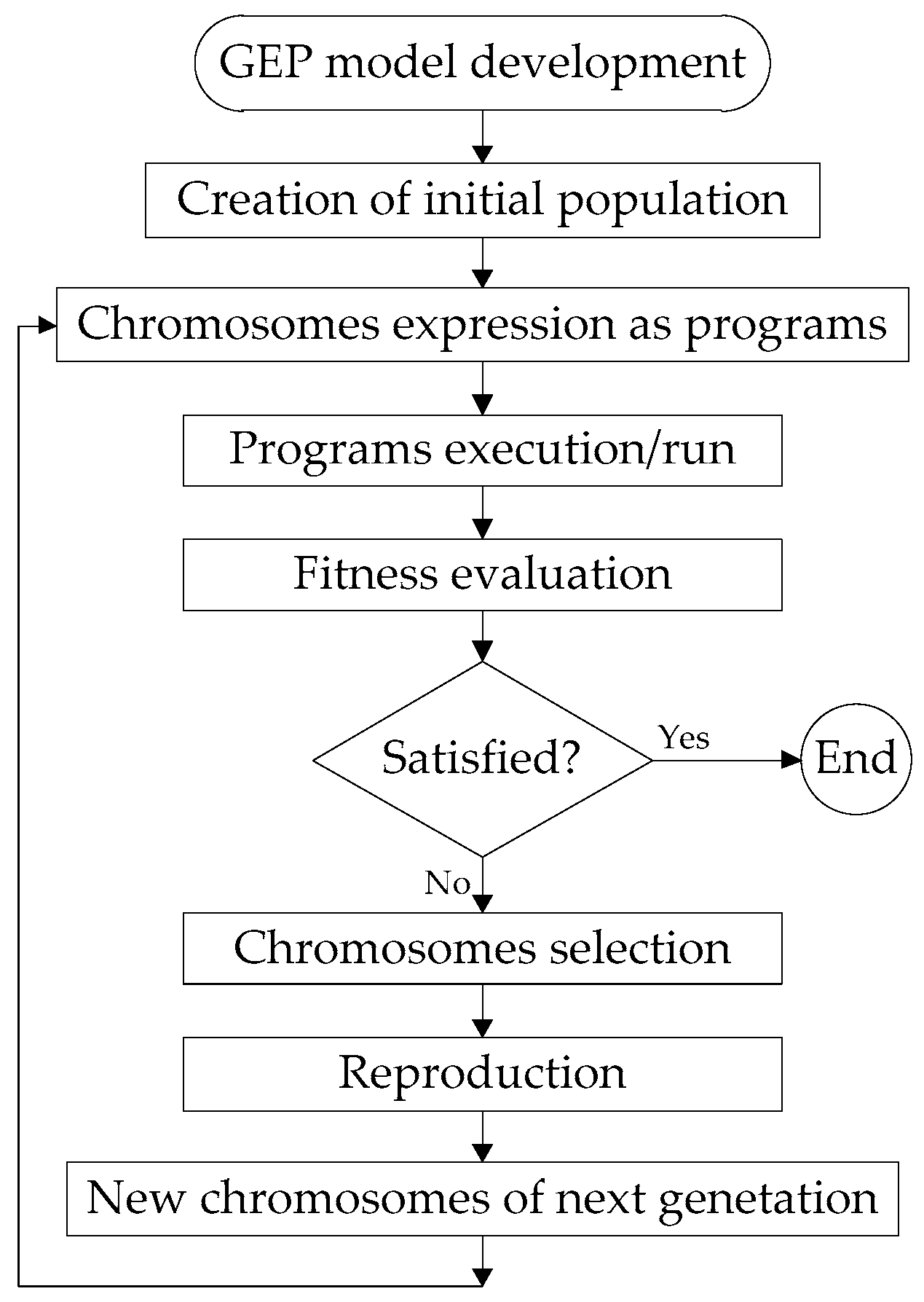
The GEP algorithm was proposed by Ferreira et al., in 2001 by combining the long linear symbol coding of gene algorithm (GA) and the algorithm established by gene programming (GP) to solve the advantages of complex nonlinear problems [43]. A typical GEP begins with a primary race and undergoes a continuous evolutionary process, including selection, replication, mating, mutation, adaptation, reversal, and transformation, to evolve toward a predetermined objective. It improves the shortcomings of GA, including premature convergence and combined explosion; further, its evolution rate is more than 100 times higher than that of GA and GP [44]. Typically, the GEP model developing could divide into 2 phases, which are called training and validation. Around 70% of the data were used in the model training phase; the last 30% of data were used for model validation. After the model was developed, the model could be applied for model applicability test. The following flow chart describes the GEP model developing and calculation process, as depicted in Figure 4 [45].

The coding rules of the GEP algorithm are similar to those of the GA, which use the equal-length linear symbols to form a “gene”, and one or more genes subsequently combined into a “chromosome”. Among them, the gene position can be placed along with different types of nodes, including function nodes and terminal nodes; further, the function nodes can be either arithmetic or logical operators and comparison operators, and the terminal nodes can be custom variables or constants, the construction of a chromosome is presented in

Table 2. The construction of a chromosome.

Head			Tail
0	1	2	3	4	5	6
AND	>	<	E	2	F	3

[46].

The structure of each chromosome is divided into at least a head and a tail, among which the head contains its function node and terminal node and the tail contains only its terminal node; further, the tail gene number is related to the head. The function can be stated as Equation (2).

$$t=h\times \left(n_{max}-1\right)+1$$

(2)

where, t is the tail gene numbers; h is the head gene numbers; n_max is the largest breach amount. In Table 2, h = 3 and n_max = 2, t = 3 × 1 + 1 = 4.

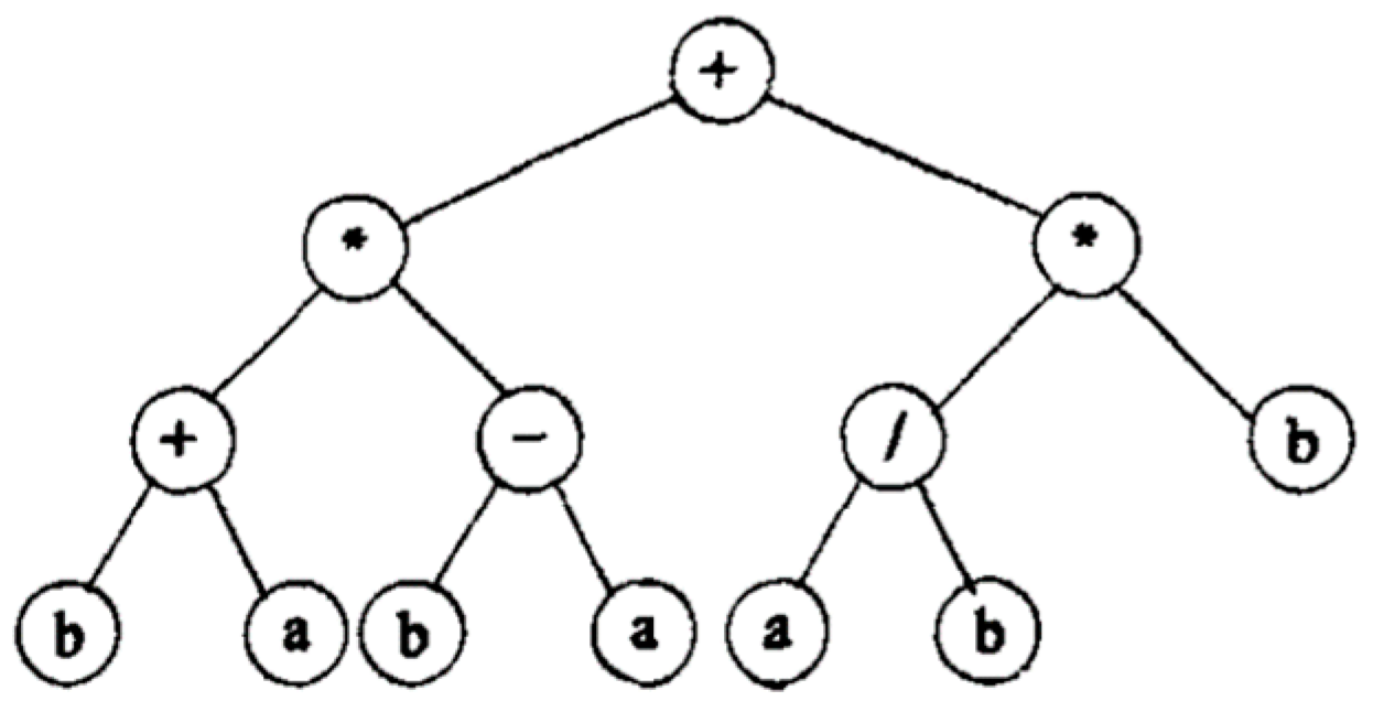
According to the gene-binding chromosome, a tree structure can be established, which can be referred to as a gene-expression tree. As depicted in Figure 5, the expression of the chromosome can be obtained according to the rules of top-down and left-right. By considering the gene-expression tree as an example, the expression of this gene can denote in Equation (3).

$$\left[\left(b+a\right)\times \left(b-a\right)\right]+\left[\left(a/b\right)\times b\right]$$

(3)

2.4. Accuracy Assessment

The accuracy determines the model performance. This study evaluates the accuracy of the MLR and the GEP model according to the methods used by Petus, C. et al., and Gohin, F. et al. [41,47]. Among them, R² was used to denote the ability for estimating the ratio of model variation concerning all the variants. The larger R² is able to explain the proportion of total variation, the higher R² is the amount of explanatory power possessed by this model. However, because R² is susceptible to extreme values, it may result in R² becoming close to 1, but most of the simulation results are entirely different from the actual turbidity. The RMSE was calculated for evaluating the error to avoiding that situation. The difference between the RMSE and the actual turbidity average is evaluated using R-RMSE to compare the rationality of the simulation results of the two models. The accuracy evaluation formula used in this study listed in Equations (4)–(8).

Moreover, the model practicability evaluation is considering of the drinking water critical turbidity (5 NTU) [48]. The turbidity data which over 5 NTU were extracted and compared for the model simulation capability examination in critical turbidity situation. The absolute error, R², RMSE, and R-RMSE were used in critical turbidity simulation assessment. Finally, the models’ simulation ability were rated refer to Heinemann, A. B. et al., Li, M. F. et al., and Despotovic, M. et al., used R-RMSE to evaluate the model performance [49,50,51]. In these studies, R-RMSE was divided into 4 intervals, when R-RMSE is less than 10%, it is considered to be outstanding, whereas it is considered to be good when R-RMSE is between 10% and 20%. Furthermore, when R-RMSE is between 20% and 30%, it is considered to be normal, and it is considered to be bad when R-RMSE is higher than 30%.

$$R^2=\frac{S{S}_{Regression}}{S{S}_{Total}}$$

(4)

$$S{S}_{Regression}={{\displaystyle \sum }}_{i=1}^n{\left({\widehat{y}}_i-\overline{y}\right)}^2$$

(5)

$$S{S}_{Total}={{\displaystyle \sum }}_{i=1}^n{\left(y_i-\overline{y}\right)}^2$$

(6)

$$RMSE=\sqrt{\frac{{{\displaystyle \sum }}_{i=1}^n{\left(y_i-{\widehat{y}}_i\right)}^2}{n-1}}$$

(7)

$$R\text{-}RMSE(\%)=\frac{RMSE}{\overline{y}}\times 100$$

(8)

where R² is a coefficient of determination, SS_Regression is the variances of each model, SS_Total is the variances of observed data, ${\widehat{y}}_i$ is predicted value of each model, $y_i$ is observed data, $\overline{y}$ is the mean of the observed data, n is the number of observed data, RMSE is the root mean square error, R-RMSE is the relative root mean square error.

3. Results and Discussion

First, the measured turbidity was sorted, and the spectral data were matched and processed with measured turbidity data. Further, the MLR and GEP turbidity simulation models could be developed by the data from Tseng-Wen reservoir and those models adopted in Nan-Hwa reservoir to test the model applicability. Finally, models’ performance was conducted by accuracy assessment.

3.1. Data Collection

This study collected the measured turbidity data and the Landsat 8 satellite imagery since October 2013 at the Tseng-Wen and January 2015 at the Nan-Hwa reservoir. According to the corresponding research area of Landsat 8 satellite, the flight route number (117/44 and 118/44), and its shooting period (once per 16 days), the time when the satellite shooting study area can be calculated, the detail information of collected Landsat 8 satellite imagery is shown in

Table 3. The information on selected Landsat 8 satellite imagery.

Reservoirs	Date	Path	Landsat Scene ID	Stations	Number of Samples
Tseng-Wen	2013/10/25	117/44	LC81170442013298LGN01	TW 1, 3, 4, 5, 6	5
	2014/11/04	118/44	LC81180442014308LGN01	TW 1, 2, 3, 4, 6	5
	2015/01/23	118/44	LC81180442015023LGN01	TW 1, 2, 3, 4, 5, 6	6
	2015/05/08	117/44	LC81170442015128LGN01	TW 2, 3, 4	3
	2015/07/18	118/44	LC81170442015128LGN01	TW 1, 2, 3, 4, 5, 6	6
	2016/01/19	117/44	LC81170442016019LGN02	TW 1, 3, 4, 6	4
	2016/11/09	118/44	LC81180442016314LGN01	TW 1, 2, 3, 4, 5, 6	6
	2017/01/12	118/44	LC81180442017012LGN01	TW 1, 2, 3	3
	2017/02/06	117/44	LC81170442017037LGN00	TW 1, 2, 3, 4, 5, 6	6
	2017/06/21	118/44	LC81180442017172LGN00	TW 1, 2, 3, 4, 5, 6	6
	2017/08/17	117/44	LC81170442017229LGN00	TW 2, 3, 4, 5, 6	5
Nan-Hwa	2015/01/23	118/44	LC81180442015023LGN01	NH 1, 2	2
	2016/03/30	118/44	LC81180442016090LGN01	NH 1	1
	2016/04/08	117/44	LC81170442016099LGN01	NH 1	1
	2016/08/05	118/44	LC81180442016218LGN01	NH 1	1
	2016/12/04	117/44	LC81170442016339LGN01	NH 1	1
	2016/12/11	118/44	LC81180442016346LGN01	NH 1	1
	2017/01/12	118/44	LC81180442017012LGN01	NH 1	1
	2017/01/28	118/44	LC81180442017028LGN00	NH 1	1
	2017/02/06	117/44	LC81170442017037LGN00	NH 1, 2	2
	2017/02/13	118/44	LC81180442017044LGN00	NH 1	1
	2017/06/30	117/44	LC81170442017181LGN00	NH 1	1
	2017/10/11	118/44	LC81180442017284LGN00	NH 1	1
	2017/10/20	117/44	LC81170442017293LGN00	NH 1	1
	2017/10/27	118/44	LC81180442017300LGN00	NH 1	1
	2017/11/21	117/44	LC81170442017325LGN00	NH 1	1
	2017/11/28	118/44	LC81180442017332LGN00	NH 1	1

.

In the pairing of measured turbidity data and satellite spectral data obtained from the Tseng-Wen reservoir, after the processing (such as cloud coverage) data were deleted, totally 55 matched turbidity and spectral data were available for the turbidity simulation model developing, the lowest turbidity is 0.95 NTU, and the highest turbidity is 21 NTU. According to the same procedure, there are 18 paired turbidity and spectral data in the model testing area Nan-Hwa reservoir, the lowest turbidity is 1.7 NTU, and the highest turbidity is 6.1 NTU.

3.2. Simulated Turbidity by Multiple Linear Regression (MLR) Model

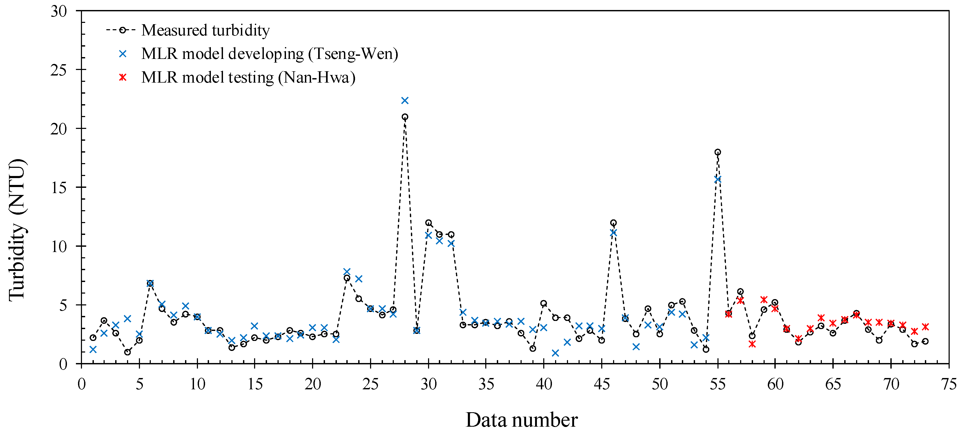
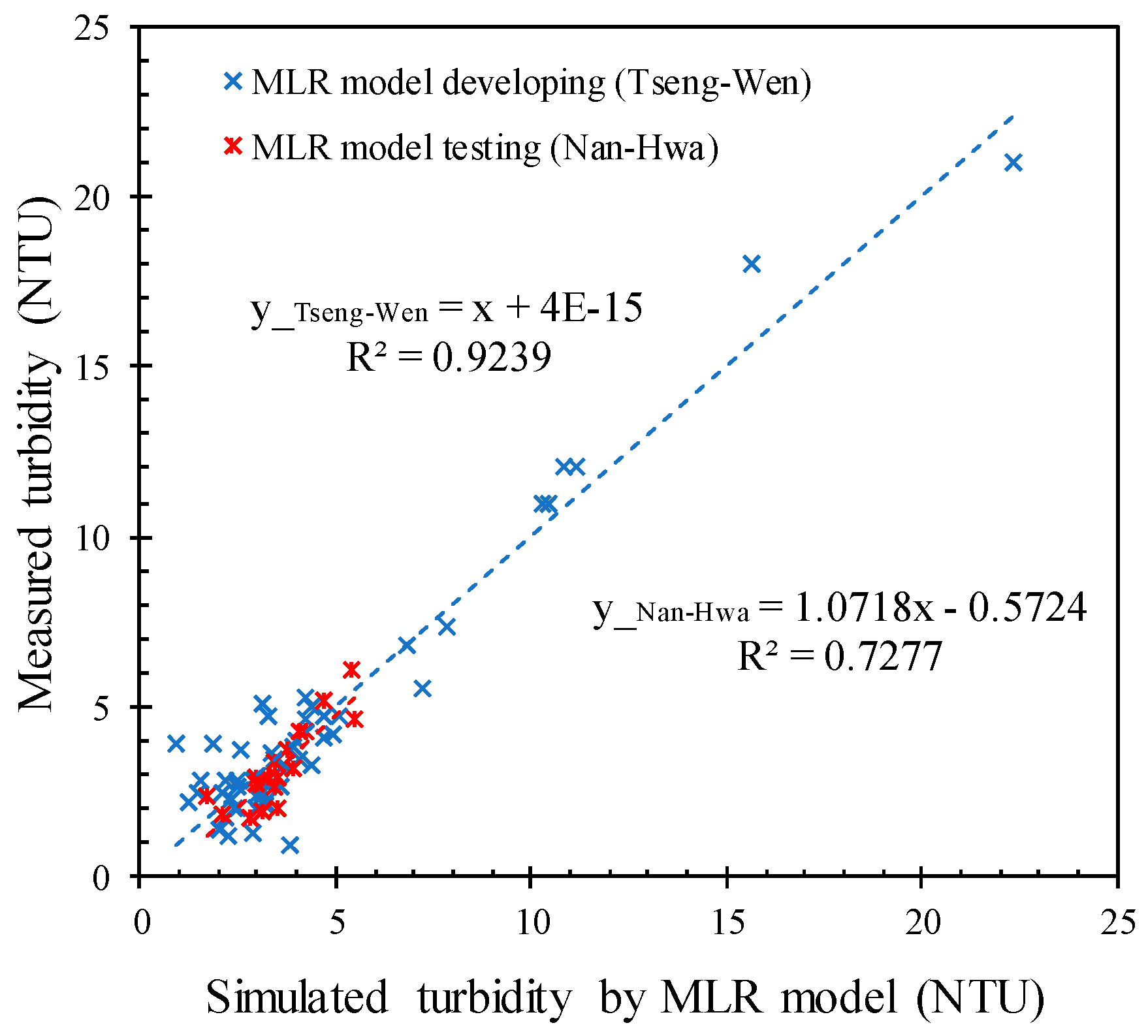
Developed MLR turbidity simulation model was given as Equation (9). Applying the spectral data into Equation (9) for turbidity simulation, a relationship between observed and simulated turbidity could be drawn in Figure 6, and the correlation relation could be drawn in Figure 7.

$$\mathrm{MLR}=-74.26B2-14.84B3+267.45B4-126.89B5+4.21$$

(9)

where, MLR is the turbidity simulation equation of MLR model; B2, B3, B4, B5 are bands from band 2 to band 5 of Landsat 8 satellite.

3.3. Simulated Turbidity by Gene-Expression Programming (GEP) Model

In the GEP model, the number of chromosomes is 50, the head size is 7, and the number of genes is 4. Only use the essential operation elements including +, −, ×, ÷, 1/x, −x, x, x² to avoid building a complicated model, and reduce the number of pattern iteration operations and the number of non-convergence occurrences. Furthermore, based on GEP algorithm, the gene-expression trees were developed and connected to sub gene-expression trees by multiplication. The parameters of the GEP turbidity simulation model are listed in

Table 4. The construction of a chromosome.

Chromosomes	Head Size	Genes	Linking Function	Calculation Functions
50	7	4	Multiplication	+, -, *, /, 1/x, -x, x, x2

.

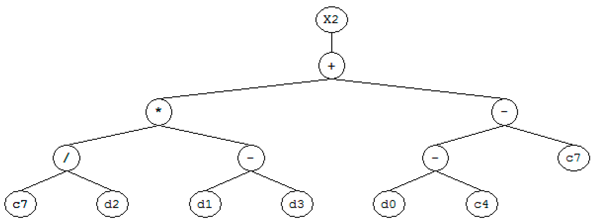
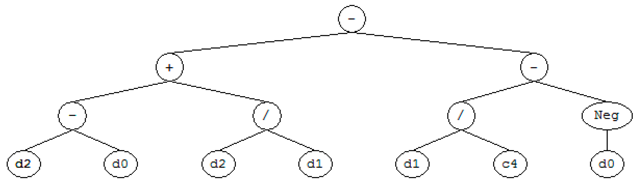
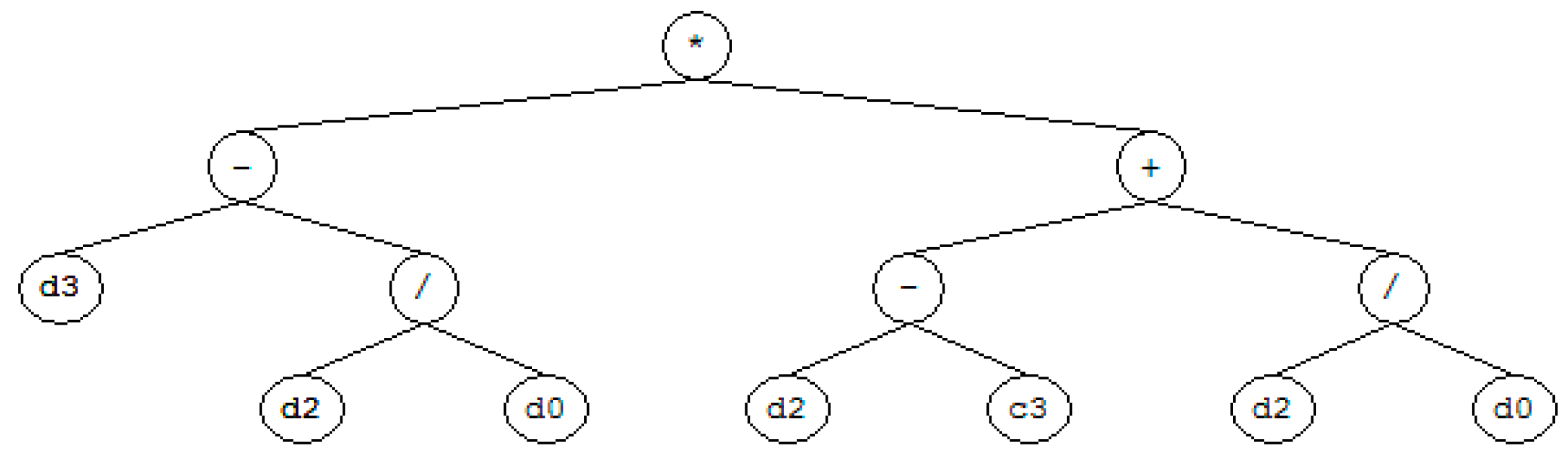
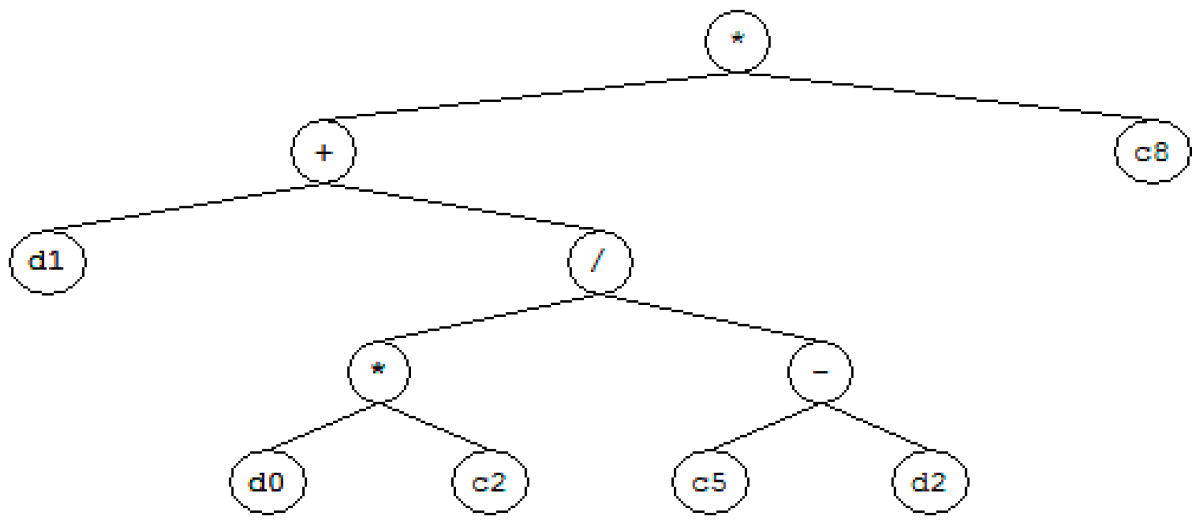
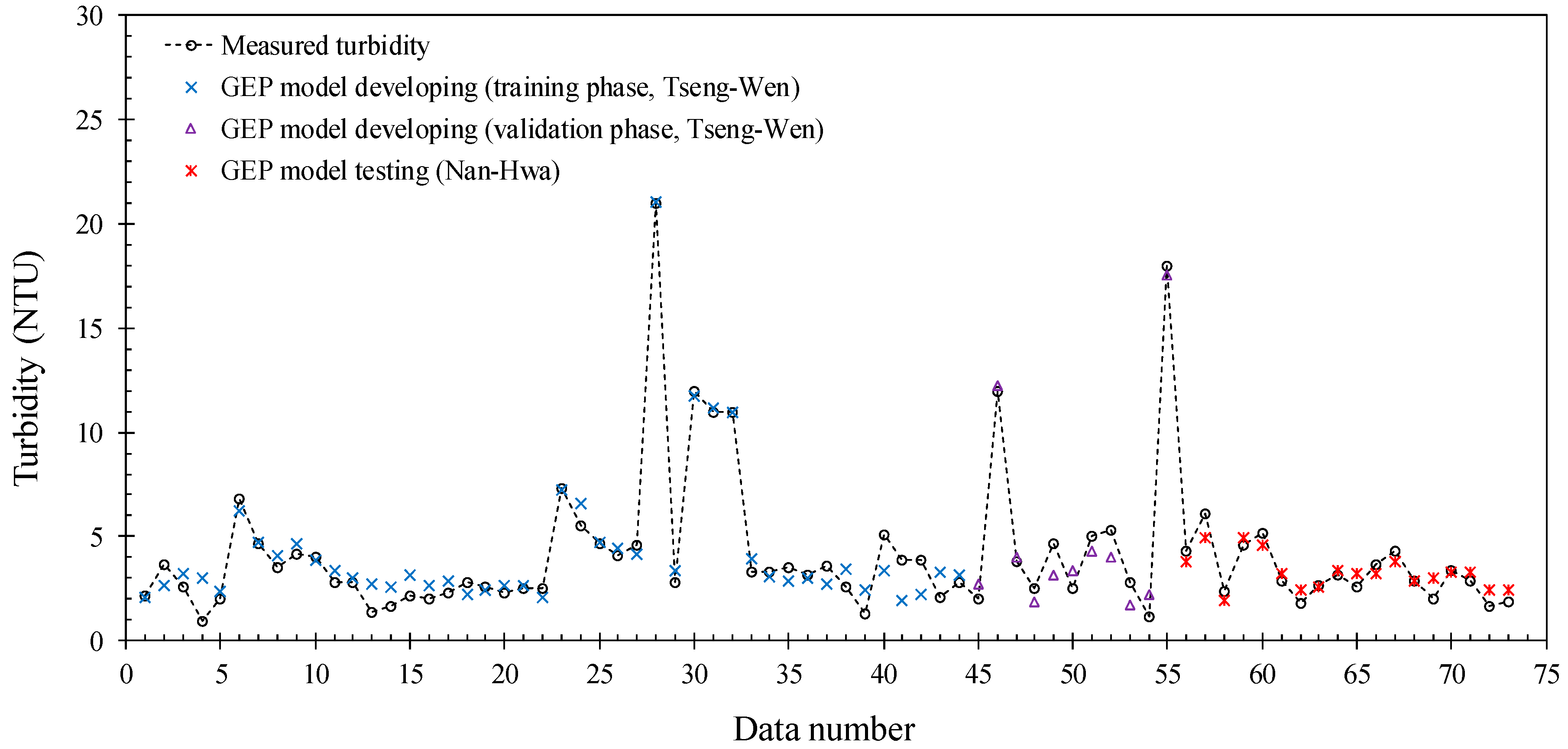
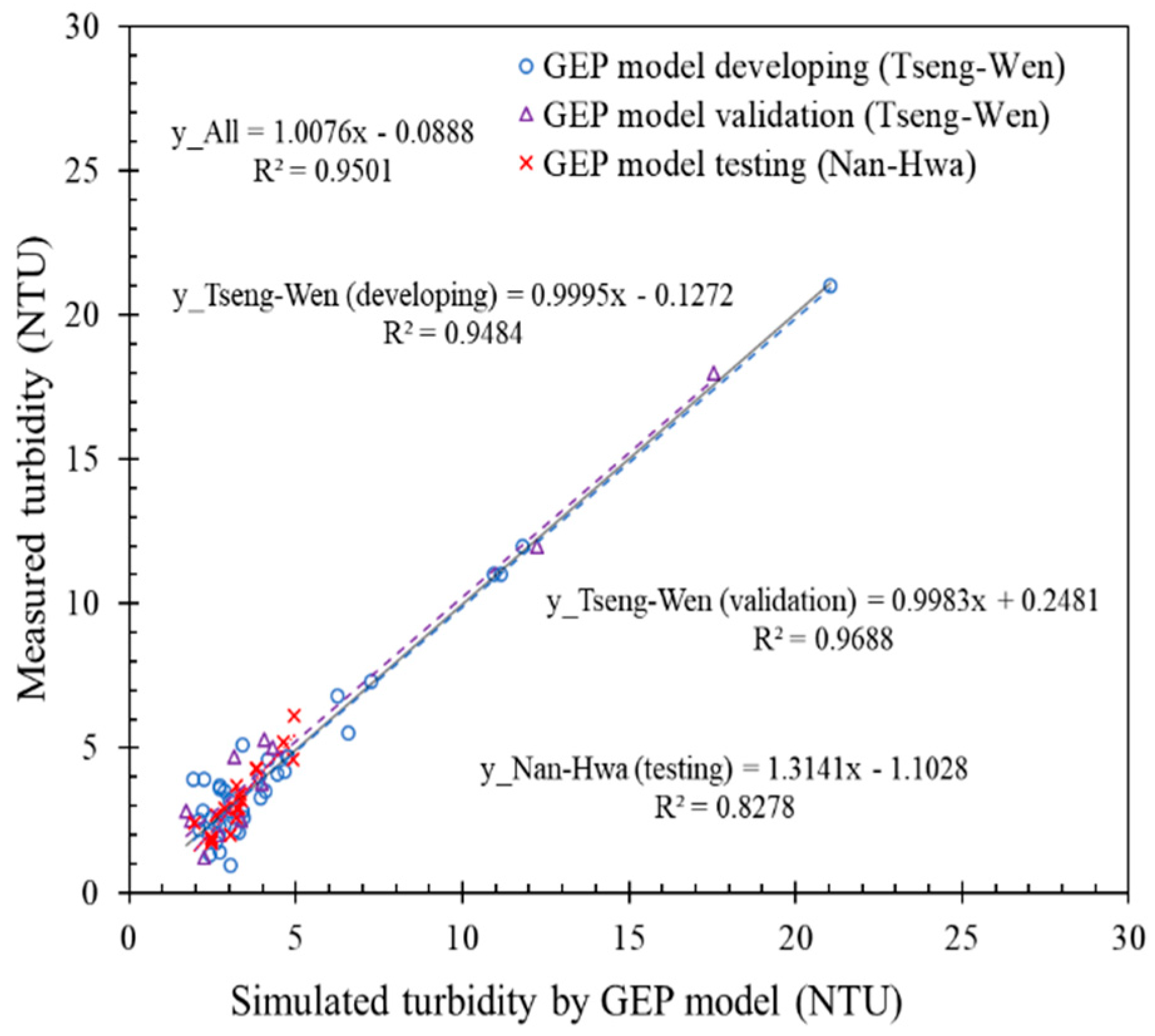
In this study, 4 sub gene-expression trees were developed, all the sub gene-expression trees were drawn in Figure 8, Figure 9, Figure 10 and Figure 11, and the turbidity simulation model was given in Equations (10) to (14). Further, the GEP model was applied to the Nan-Hwa reservoir. The relationship and the correlation of simulated turbidity and measured turbidity of the Tseng-Wen reservoir and the Nan-Hwa reservoir, which are inferred from the GEP model, are presented in Figure 12 and Figure 13.

$$GEP=E{T}_{sub1}\times E{T}_{sub2}\times E{T}_{sub3}\times E{T}_{sub4}$$

(10)

$$E{T}_{sub1}={\left\{\frac{c7}{d2}\times \left(d1-d3\right)+\left[d0-\left(c4\right)\right]-c7\right\}}^2={\left\{3.1095\times \frac{\left(B2-B4\right)}{B3}+B1+2.1116\right\}}^2$$

(11)

$$E{T}_{sub2}=\left(d2-d0\right)\times \frac{d2}{d1}-\left[\frac{d1}{c4}-\left(-d0\right)\right]=\left(B3-B1\right)\times \frac{B3}{B2}-\frac{B2}{3.9763}+B1$$

(12)

$$E{T}_{sub3}=\left(d3-\frac{d2}{d0}\right)\times \left(d2-c3+\frac{d2}{d0}\right)=\left(B4-\frac{B3}{B1}\right)\times \left(B3-0.065+\frac{B3}{B1}\right)$$

(13)

$$E{T}_{sub4}=\left[d1+(\frac{d0\times c2}{c5-d2})\right]\times c8=\left[B2+(\frac{B1\times 3.1024}{5.0160-B3})\right]\times -7.4847$$

(14)

where, ET_sub1, ET_sub2, ET_sub3, and ET_sub4 are the 1st to 4th sub gene-expression tree, respectively; d0, d1, d2, d3 correspond to Landsat 8 satellite band 2 to band 5; c0~c9 are constants, in ET_sub1, c4 = −5.2211, c7 = 3.1095; in ET_sub2, c4 = 3.9763; in ET_sub3, c3 = 0.065; in ET_su4, c2 = 3.1024, c5 = 5.0160, c8 = −7.4847.

3.4. Simulated Turbidity Accuracy Assessment

The model performance was evaluated according to R², RMSE, and R-RMSE in the MLR model developing, MLR model testing, GEP model developing (training phase and validating phase), and GEP model testing, respectively. According to the calculation results, the R² of the MLR model developing and testing is 0.9181 and 0.7277, respectively, the RMSE is 1.0726 NTU and 0.7248 NTU, respectively, and the R-RMSE are 24.08% and 22.26%, respectively. In the GEP model, the R² of the model training phase, validating phase, and model testing are 0.9484, 0.9688, and 0.8278, respectively, and the RMSE are 0.8190 NTU, 0.9315 NTU, and 0.5815 NTU, respectively. The R-RMSE are 19.46%, 17.13%, and 17.86%, respectively. The calculated results are present in

Table 5. The accuracy assessment table of multiple linear regression (MLR) and gene-expression programming (GEP) models.

	MLR			GEP
	R2	RMSE	R-RMSE	R2	RMSE	R-RMSE
		(NTU)	(%)		(NTU)	(%)
Model developing (Tseng-Wen)	0.9239	1.0726	24.08%	0.9484 1	0.8190 1	19.46% 1
				0.9688 2	0.9315 2	17.13% 2
Model testing (Nan-Hwa)	0.7277	0.7248	22.26%	0.8278	0.5815	17.86%

¹ The training phase of GEP model developing. ² The validating phase of GEP model developing.

. The model accuracy assessment result indicates that the simulated error of GEP model is lower than the MLR model.

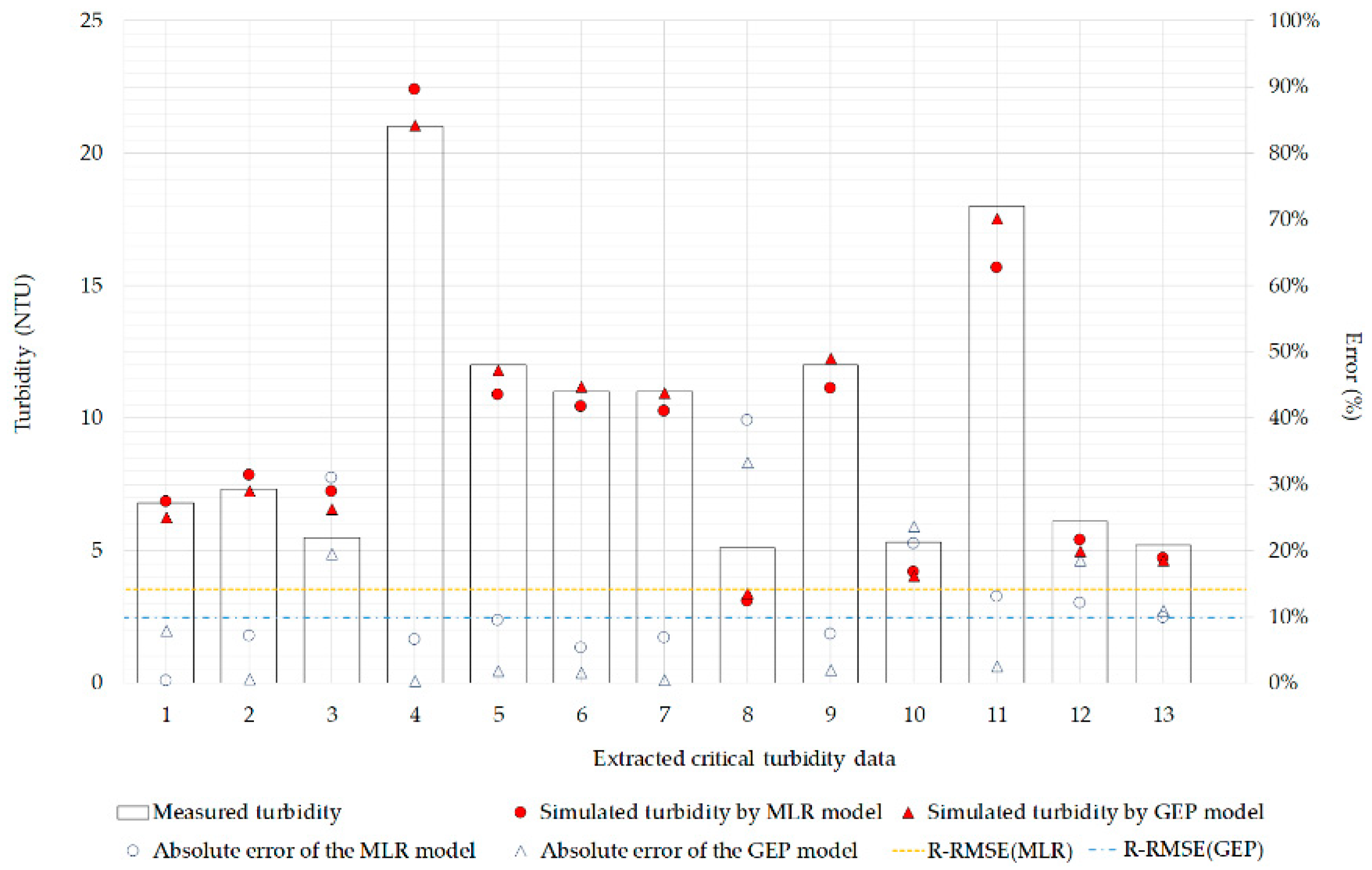
Considering the drinking water supply commendation which was suggested by WHO [48], the maximum turbidity for drinking water cannot exceed 5 NTU; thus, this study compares the critical turbidity data (over 5 NTU) from measured turbidity and simulated turbidity, to figure out the model simulation ability in critical turbidity condition. In total, 13 critical turbidity data were extracted, ranging from 5.1 NTU to 21 NTU, with the absolute error of the MLR and GEP between 0.294% to 39.608%, 0.240% to 33.333%, respectively. In the critical turbidity condition comparison, the R², RMSE, and R-RMSE of the MLR model are 0.9507, 1.2284, and 13.32%, respectively, and the R², RMSE, and R-RMSE of the GEP model are 0.9837, 0.7766, and 8.28%, respectively. The critical turbidity comparison result is shown in

Table 6. The model comparison of critical turbidity condition.

	MLR			GEP
	R2	RMSE	R-RMSE	R2	RMSE	R-RMSE
		(NTU)	(%)		(NTU)	(%)
Critical turbidity (> 5 NTU)	0.9507	1.2284	13.32%	0.9837	0.7766	8.28%

and Figure 14. According to the result of critical turbidity comparison, the simulated turbidity by the GEP model is more precise than the MLR model, which means in critical turbidity condition (>5 NTU), the simulation error of the GEP model is less than the MLR model.

Finally, this study refers to Heinemann et al., Li et al., and Despotovic, et al., used R-RMSE to evaluate the model performance [49,50,51]. In these studies, R-RMSE was divided into 4 intervals, when R-RMSE is less than 10%, it is considered to be outstanding, whereas it is considered to be good when R-RMSE is between 10% and 20%. Further, when R-RMSE is between 20% and 30%, it is considered to be normal, and it is considered to be bad when R-RMSE is higher than 30%. In this study, the turbidity simulation results of the GEP model developing (including training phase and validation phase) and testing, are considered to be good. Moreover, in the critical turbidity condition, the simulated result even belongs to an outstanding level, exhibiting that the simulated turbidity of the GEP model is relatively reliable and reasonable than the MLR model.

4. Conclusions

This study collected the in-situ turbidity of Tseng-Wen and Nan-Hwa reservoir paired with Landsat 8 satellite spectrum imagery of the uncovered study area, to develop and test the turbidity simulation model. In total, 55 measured turbidity data obtained from the Tseng-Wen reservoir were used for model developing, and 18 turbidity data obtained from the Nan-Hwa reservoir for model testing. The MLR model and the GEP model were selected to establish the turbidity model, and the R², RMSE, and R-RMSE were used for model accuracy assessment. The research result can be divided into 3 parts, includes accuracy assessment comparison, critical turbidity comparison, and the model performance evaluation by R-RMSE.

First, in accuracy assessment comparison, the R², RMSE, and R-RMSE of MLR and GEP are 0.7277 and 0.8278, 0.7248 NTU and 0.5815 NTU, 22.26% and 17.86%, respectively. The assessment results of the GEP model are more accurate than the MLR model.

Secondly, in critical turbidity condition comparison, the critical turbidity condition was given (>5NTU) by WHO [48]. In 13 critical turbidity data, the mean absolute error is 3.55%, the R², RMSE, and R-RMSE of the MLR and the GEP model is 0.9507 and 0.9837, 1.2284 and 0.7766, 13.32% and 8.28%, respectively. The simulated turbidity by GEP model is more convincible than MLP model in the critical turbidity condition.

Finally, R-RMSE was used to evaluate the model performance 4 stages were divided, including outstanding, good, normal, and bad when the R-RMSE in the range of less than 10%, between 10% and 20%, between 20% and 30%, and over 30%, respectively. The phase of developing and testing of the MLR model ware considered to be normal. In the GEP model developing and testing phases, were ranked as good. Moreover, in the critical turbidity condition, the simulated result even belongs to the outstanding level of the GEP model, exhibiting the fact that the simulated turbidity of the GEP model is relatively reliable and reasonable than the MLR model.

Base on the result of this study, no sufficient change is observed in the simulated turbidity results of the testing area. Although it may be different because of the characteristics of the catchment and geology, the comparison results exhibit that the GEP turbidity simulation model established in this study denotes individual turbidity simulation rationality and indicates that the GEP turbidity simulation model exhibits relatively good applicability. It can be concluded from this study that the GEP algorithm is suitable for empirical turbidity simulation model developing, and the modeling results from the GEP model are accurate enough for reservoir surface water turbidity estimation.

References

- EPA. Water Turbidity Test Standard-Turbiditymeter Method (niea w219.52); Environmental Protection Administration: Taipei, Taiwan, 2005; pp. 1–4.
- Yang, M.; Sykes, R.; Merry, C. Estimation of algal biological parameters using water quality modeling and SPOT satellite data. Ecol. Model. 2000, 125, 1–13. [Google Scholar] [CrossRef]
- Kallio, K.; Kutser, T.; Hannonen, T.; Koponen, S.; Pulliainen, J.; Vepsäläinen, J.; Pyhälahti, T. Retrieval of water quality from airborne imaging spectrometry of various lake types in different seasons. Sci. Total Environ. 2001, 268, 59–77. [Google Scholar] [CrossRef]
- Roelfsema, C.; Phinn, S.; Dennison, W.; Dekker, A.; Brando, V.E. Monitoring toxic cyanobacteria Lyngbya majuscula (Gomont) in Moreton Bay, Australia by integrating satellite image data and field mapping. Harmful Algae 2006, 5, 45–56. [Google Scholar] [CrossRef]
- Robert, E.; Grippa, M.; Kergoat, L.; Pinet, S.; Gal, L.; Cochonneau, G.; Martinez, J.-M. Monitoring water turbidity and surface suspended sediment concentration of the Bagre Reservoir (Burkina Faso) using MODIS and field reflectance data. Int. J. Appl. Earth Obs. Geoinf. 2016, 52, 243–251. [Google Scholar] [CrossRef]
- Chen, S.; Fang, L.; Zhang, L.; Huang, W. Remote sensing of turbidity in seawater intrusion reaches of Pearl River Estuary–A case study in Modaomen water way, China. Estuar. Coast. Shelf Sci. 2009, 82, 119–127. [Google Scholar] [CrossRef]
- Miller, R.L.; McKee, B.A. Using MODIS Terra 250 m imagery to map concentrations of total suspended matter in coastal waters. Remote Sens. Environ. 2004, 93, 259–266. [Google Scholar] [CrossRef]
- Doxaran, D.; Froidefond, J.-M.; Lavender, S.; Castaing, P. Spectral signature of highly turbid waters: Application with SPOT data to quantify suspended particulate matter concentrations. Remote Sens. Environ. 2002, 81, 149–161. [Google Scholar] [CrossRef]
- Min, J.-E.; Ryu, J.-H.; Lee, S.; Son, S. Monitoring of suspended sediment variation using Landsat and MODIS in the Saemangeum coastal area of Korea. Mar. Pollut. Bull. 2012, 64, 382–390. [Google Scholar] [CrossRef]
- Gordon, H.R.; Clark, D.K.; Brown, J.W.; Brown, O.B.; Evans, R.H.; Broenkow, W.W. Phytoplankton pigment concentrations in the Middle Atlantic Bight: Comparison of ship determinations and CZCS estimates. Appl. Opt. 1983, 22, 20–36. [Google Scholar] [CrossRef]
- Chebud, Y.; Naja, G.M.; Rivero, R.G.; Melesse, A.M. Water quality monitoring using remote sensing and an artificial neural network. Water Air Soil Pollut. 2012, 223, 4875–4887. [Google Scholar] [CrossRef]
- Ng, W.-T.; Rima, P.; Einzmann, K.; Immitzer, M.; Atzberger, C.; Eckert, S. Assessing the Potential of Sentinel-2 and Pléiades Data for the Detection of Prosopis and Vachellia spp. in Kenya. Remote Sens. 2017, 9, 74. [Google Scholar] [CrossRef]
- Kawamura, K.; Ikeura, H.; Phongchanmaixay, S.; Khanthavong, P. Canopy Hyperspectral Sensing of Paddy Fields at the Booting Stage and PLS Regression can Assess Grain Yield. Remote Sens. 2018, 10, 1249. [Google Scholar] [CrossRef]
- Lebourgeois, V.; Dupuy, S.; Vintrou, É.; Ameline, M.; Butler, S.; Bégué, A. A Combined Random Forest and OBIA Classification Scheme for Mapping Smallholder Agriculture at Different Nomenclature Levels Using Multisource Data (Simulated Sentinel-2 Time Series, VHRS and DEM). Remote Sens. 2017, 9, 259. [Google Scholar] [CrossRef]
- Atzberger, C.; Guérif, M.; Baret, F.; Werner, W. Comparative analysis of three chemometric techniques for the spectroradiometric assessment of canopy chlorophyll content in winter wheat. Comput. Electron. Agric. 2010, 73, 165–173. [Google Scholar] [CrossRef]
- Thanh Noi, P.; Kappas, M. Comparison of Random Forest, k-Nearest Neighbor, and Support Vector Machine Classifiers for Land Cover Classification Using Sentinel-2 Imagery. Sensors 2017, 18, 18. [Google Scholar] [CrossRef] [PubMed]
- Ferrant, S.; Selles, A.; Le Page, M.; Herrault, P.-A.; Pelletier, C.; Al-Bitar, A.; Mermoz, S.; Gascoin, S.; Bouvet, A.; Saqalli, M.; et al. Detection of Irrigated Crops from Sentinel-1 and Sentinel-2 Data to Estimate Seasonal Groundwater Use in South India. Remote Sens. 2017, 9, 1119. [Google Scholar] [CrossRef]
- Pandit, S.; Tsuyuki, S.; Dube, T. Estimating Above-Ground Biomass in Sub-Tropical Buffer Zone Community Forests, Nepal, Using Sentinel 2 Data. Remote Sens. 2018, 10, 601. [Google Scholar] [CrossRef]
- Novák, J.; Lukas, V.; Křen, J. Estimation of Soil Properties Based on Soil Colour Index. Agric. Conspec. Sci. 2018, 83, 71–76. [Google Scholar]
- Sothe, C.; Almeida, C.; Liesenberg, V.; Schimalski, M. Evaluating Sentinel-2 and Landsat-8 Data to Map Sucessional Forest Stages in a Subtropical Forest in Southern Brazil. Remote Sens. 2017, 9, 838. [Google Scholar] [CrossRef]
- Immitzer, M.; Vuolo, F.; Atzberger, C. First Experience with Sentinel-2 Data for Crop and Tree Species Classifications in Central Europe. Remote Sens. 2016, 8, 166. [Google Scholar] [CrossRef]
- Liu, Y.; Gong, W.; Hu, X.; Gong, J. Forest Type Identification with Random Forest Using Sentinel-1A, Sentinel-2A, Multi-Temporal Landsat-8 and DEM Data. Remote Sens. 2018, 10, 946. [Google Scholar] [CrossRef]
- Mohite, J.; Trivedi, M.; Surve, A.; Sawant, M.; Urkude, R.; Pappula, S. Hybrid classification-clustering approach for export-non export grape area mapping and health estimation using sentinel-2 satellite data. In Proceedings of the 2017 6th International Conference on Agro-Geoinformatics, Fairfax, VA, USA, 7–10 August 2017; pp. 1–6. [Google Scholar]
- Ramoelo, A.; Cho, M.A.; Mathieu, R.; Madonsela, S.; van de Kerchove, R.; Kaszta, Z.; Wolff, E. Monitoring grass nutrients and biomass as indicators of rangeland quality and quantity using random forest modelling and WorldView-2 data. Int. J. Appl. Earth Obs. Geoinf. 2015, 43, 43–54. [Google Scholar] [CrossRef]
- Filgueiras, R.; Mantovani, E.C.; Dias, S.H.B.; Fernandes Filho, E.I.; Cunha, F.F.d.; Neale, C.M.U. New approach to determining the surface temperature without thermal band of satellites. Eur. J. Agron. 2019, 106, 12–22. [Google Scholar] [CrossRef]
- Xiong, J.; Thenkabail, P.; Tilton, J.; Gumma, M.; Teluguntla, P.; Oliphant, A.; Congalton, R.; Yadav, K.; Gorelick, N. Nominal 30-m Cropland Extent Map of Continental Africa by Integrating Pixel-Based and Object-Based Algorithms Using Sentinel-2 and Landsat-8 Data on Google Earth Engine. Remote Sens. 2017, 9, 1065. [Google Scholar] [CrossRef]
- Richter, K.; Hank, T.B.; Vuolo, F.; Mauser, W.; D’Urso, G. Optimal Exploitation of the Sentinel-2 Spectral Capabilities for Crop Leaf Area Index Mapping. Remote Sens. 2012, 4, 561–582. [Google Scholar] [CrossRef] [Green Version]
- Ramoelo, A.; Cho, M.; Mathieu, R.; Skidmore, A.K. Potential of Sentinel-2 spectral configuration to assess rangeland quality. J. Appl. Remote Sens. 2015, 9, 094096. [Google Scholar] [CrossRef]
- Sakowska, K.; Juszczak, R.; Gianelle, D. Remote Sensing of Grassland Biophysical Parameters in the Context of the Sentinel-2 Satellite Mission. J. Sens. 2016, 2016, 4612809. [Google Scholar] [CrossRef]
- Sitokonstantinou, V.; Papoutsis, I.; Kontoes, C.; Arnal, A.; Andrés, A.P.; Zurbano, J.A. Scalable Parcel-Based Crop Identification Scheme Using Sentinel-2 Data Time-Series for the Monitoring of the Common Agricultural Policy. Remote Sens. 2018, 10, 911. [Google Scholar] [CrossRef]
- Belgiu, M.; Csillik, O. Sentinel-2 cropland mapping using pixel-based and object-based time-weighted dynamic time warping analysis. Remote Sens. Environ. 2018, 204, 509–523. [Google Scholar] [CrossRef]
- Van Tricht, K.; Gobin, A.; Gilliams, S.; Piccard, I. Synergistic Use of Radar Sentinel-1 and Optical Sentinel-2 Imagery for Crop Mapping: A Case Study for Belgium. Remote Sens. 2018, 10, 1642. [Google Scholar] [CrossRef]
- Atzberger, C.; Richter, K.; Vuolo, F.; Darvishzadeh, R.; Schlerf, M. Why confining to vegetation indices? Exploiting the potential of improved spectral observations using radiative transfer models. In Proceedings of the Remote Sensing for Agriculture, Ecosystems, and Hydrology XIII, Prague, Czech Republic, 19–21 September 2011; SPIE: Washington, DC, USA, 2011; Volume 8174. [Google Scholar]
- Tassan, S. Local algorithms using SeaWiFS data for the retrieval of phytoplankton, pigments, suspended sediment, and yellow substance in coastal waters. Appl. Opt. 1994, 33, 2369–2378. [Google Scholar] [CrossRef] [PubMed]
- Shieh, M.-L. Application of Remote Sensing Technique on Estimating Suspended Sediment Concentration. Ph.D. Thesis, National Cheng Kung University, Tainan, Taiwan, 2009. [Google Scholar]
- Chang, C.-H.; Liu, C.-C.; Wen, C.-G.; Cheng, I.-F.; Tam, C.-K.; Huang, C.-S. Monitoring reservoir water quality with Formosat-2 high spatiotemporal imagery. J. Environ. Monit. 2009, 11, 1982–1992. [Google Scholar] [CrossRef] [PubMed]
- Quang, N.H.; Sasaki, J.; Higa, H.; Huan, N.H. Spatiotemporal Variation of Turbidity Based on Landsat 8 OLI in Cam Ranh Bay and Thuy Trieu Lagoon, Vietnam. Water 2017, 9, 570. [Google Scholar] [CrossRef]
- EPA. Environmental Water Quality Information. Available online: https://wq.epa.gov.tw/Code/Default.aspx?Water=Dam (accessed on 22 May 2019).
- Ma, R.; Dai, J. Investigation of chlorophyll-a and total suspended matter concentrations using Landsat ETM and field spectral measurement in Taihu Lake, China. Int. J. Remote Sens. 2005, 26, 2779–2795. [Google Scholar] [CrossRef]
- Zhou, W.; Wang, S.; Zhou, Y.; Troy, A. Mapping the concentrations of total suspended matter in Lake Taihu, China, using Landsat-5 TM data. Int. J. Remote Sens. 2006, 27, 1177–1191. [Google Scholar] [CrossRef]
- Petus, C.; Chust, G.; Gohin, F.; Doxaran, D.; Froidefond, J.-M.; Sagarminaga, Y. Estimating turbidity and total suspended matter in the Adour River plume (South Bay of Biscay) using MODIS 250-m imagery. Cont. Shelf Res. 2010, 30, 379–392. [Google Scholar] [CrossRef] [Green Version]
- Cui, L.; Qiu, Y.; Fei, T.; Liu, Y.; Wu, G. Using remotely sensed suspended sediment concentration variation to improve management of Poyang Lake, China. Lake Reserv. Manag. 2013, 29, 47–60. [Google Scholar] [CrossRef] [Green Version]
- Ferreira, F.L.; Bota, D.P.; Bross, A.; Mélot, C.; Vincent, J.-L. Serial evaluation of the SOFA score to predict outcome in critically ill patients. JAMA 2001, 286, 1754–1758. [Google Scholar] [CrossRef]
- Ferreira, C. Gene expression programming in problem solving. In Soft Computing and Industry; Springer: Cham, Switzerland, 2002; pp. 635–653. [Google Scholar]
- Traore, S.; Luo, Y.; Fipps, G. Deployment of artificial neural network for short-term forecasting of evapotranspiration using public weather forecast restricted messages. Agric. Water Manag. 2016, 163, 363–379. [Google Scholar] [CrossRef]
- Tsai, Y.-Y. A Research on the GEP and GA Regulated Box Theory in Stock Markets. Master’s Thesis, Fu Jen Catholic University, New Taipei, Taiwan, 2016. [Google Scholar]
- Gohin, F.; Druon, J.; Lampert, L. A five channel chlorophyll concentration algorithm applied to SeaWiFS data processed by SeaDAS in coastal waters. Int. J. Remote Sens. 2002, 23, 1639–1661. [Google Scholar] [CrossRef]
- WHO. Guidelines for Drinking-Water Quality. Vol. 2, Health Criteria and Other Supporting Information: Addendum; WHO: Geneva, Switzerland, 1998. [Google Scholar]
- Heinemann, A.B.; Van Oort, P.A.; Fernandes, D.S.; Maia, A.d.H.N. Sensitivity of APSIM/ORYZA model due to estimation errors in solar radiation. Bragantia 2012, 71, 572–582. [Google Scholar] [CrossRef] [Green Version]
- Li, M.-F.; Zhang, Y.-R.; Luo, K.-H.; Wu, L.-A.; Fan, H. Time-correspondence differential ghost imaging. Phys. Rev. A 2013, 87, 033813. [Google Scholar] [CrossRef]
- Despotovic, M.; Nedic, V.; Despotovic, D.; Cvetanovic, S. Evaluation of empirical models for predicting monthly mean horizontal diffuse solar radiation. Renew. Sustain. Energy Rev. 2016, 56, 246–260. [Google Scholar] [CrossRef]
Figure 1.
Turbidity monitoring station location of (a) Tseng-Wen and (b) Nan-Hwa reservoir. (Study area satellite images were taken in 2017/11/28 by Landsat 8).
Figure 2.
Seasonal turbidity variation of Tseng-Wen reservoir and Nan-Hwa reservoir.
Figure 3.
Sediment spectrum reflectance distribution in Tseng-Wen reservoir.
Figure 4.
The flow chart of gene-expression programming (GEP) model development.
Figure 5.
The sample of the gene-expression tree.
Figure 6.
The relationship of observed turbidity and multiple linear regression (MLR) simulated turbidity in Tseng-Wen and Nan-Hwa reservoir.
Figure 7.
The correlation relationship between observed turbidity and multiple linear regression (MLR) simulated turbidity in Tseng-Wen and Nan-Hwa reservoir.
Figure 8.
The first sub gene-expression tree.
Figure 9.
The second sub gene-expression tree.
Figure 10.
The third sub gene-expression tree.
Figure 11.
The fourth sub gene-expression tree.
Figure 12.
The relation of observed turbidity and gene-expression programming (GEP) simulated turbidity in Tseng-Wen and Nan-Hwa reservoir.
Figure 13.
The correlation relationship of observed turbidity and the turbidity simulated by the gene-expression programming (GEP) model in Tseng-Wen and Nan-Hwa reservoir.
Figure 14.
The simulation error of the multiple linear regression (MLR) and the gene-expression programming (GEP) model in the critical turbidity condition.