Comparison between 2D Shallow-Water Simulations and Energy-Momentum Computations for Transcritical Flow Past Channel Contractions

Abstract

Multidimensional simulators of channel and river flow are widely used in industry and academia, raising the question about whether the classical one-dimensional theory of open-channel flow remains relevant in hydraulic engineering. Channel contractions that induce transcritical flow are interesting scenarios to test the classical 1D theory against multidimensional simulations, because supercritical flow in channels of variable width leads to multidimensional flow structures. Transcritical flows are important in practice, because the ensuing hydraulic jumps and regions of supercritical flow may damage hydraulic structures that otherwise operate under tranquil conditions. We compare well-resolved simulations of the 2D shallow-water Equations (SWE) with 1D energy-momentum calculations for flow past symmetric channel contractions. We analyze the accuracy of the classical energy-momentum gradually-varied flow theory to predict the onset of regime transitions and the location of hydraulic jumps. We test the relative performance of the 1D theory for different constriction geometries, and identify the flow mechanisms behind the discrepancies between the 1D and 2D predictions. The grid resolution used in the 2D SWE plays an important role in these predictions, because coarse-grid 2D simulations yield essentially quasi-1D results. Considering its simplicity and negligible computational cost compared with the 2D SWE simulations, the classical 1D theory performs remarkably well for a wide range of flow conditions and contraction geometries. In contrast, we observe large deviations between the 1D and 2D models in flow past abrupt contractions with a large width ratio, as expected. Only modified versions of the 1D theory, taking into account intense local head losses and the propagation of spatial flow structures downstream from the contraction, can succeed at describing these flow scenarios.

1. Introduction

The concepts of specific energy and momentum, developed by Bakhmeteff more than a century ago to describe the hydraulics of open channel flow [1,2], have been at the core of the engineering practice and curriculum in recent years [3,4]. Coupled with the equations of motion, and supplemented with models of flow resistance and assumptions of hydrostatic pressure and uniform flow across the channel width that render the problem one-dimensional, the energy-momentum theory provides an elegant and effective approach to the design of hydraulic structures and to the study of environmental flows [5,6]. Sophisticated multidimensional hydrodynamic models for free surface flow have recently become available and are widely used in industry and academia [7,8]. The possibility of conducting detailed multidimensional simulations raises the question about whether the classical theory of open channel flow remains relevant in engineering practice, or if it has rather become a back-of-the-envelope exercise aimed at developing hydraulic intuition.

Channel transitions, including expansions, contractions, channel bends or bridge piers, are incorporated into the classical theory as local features, and the associated head losses are either neglected or modeled through local energy loss terms [3,4]. Perhaps the most interesting scenarios of flow in channel transitions are those that induce changes in the flow regime—transcritical flows [9,10]—because the presence of supercritical flow regions and hydraulic jumps may have potentially damaging effects on hydraulic infrastructure that otherwise operates under tranquil flow conditions [3]. From the perspective of hydraulic design, complicating factors include the onset of spatial (two-dimensional) flow structures that dominate supercritical regions, and the possibility of near-critical scenarios leading to asymmetric flow patterns and undular hydraulic jumps [11,12,13,14].

There is a vast literature, dating back to Ippen and co-workers [15,16,17], on understanding the mechanics of high-velocity flow in open channels of variable width, with an emphasis on the design of hydraulic structures operating under supercritical conditions (e.g., the design of supercritical channel junctions [18,19] and channel expansions [20]). Recent topics in high-velocity channel flow include the possibility of multiple steady states induced by the complex shock wave interaction in supercritical flow through contractions [21], and the emergence of hysteresis in open channel flow [22,23].

The subcritical-supercritical-subcritical transition that may occur at a gradual or sudden contraction in horizontal or mildly sloped channels has been thoroughly studied since Khafagi’s seminal work on Venturi flumes [24]. For approaching supercritical flow at the channel throat, the key experimental objective has been to understand the structure of the energy dissipation mechanisms in the downstream expansion region [25,26], characterizing the flow morphology and location of hydraulic jumps in the stilling basin through the approach Froude number, expansion geometry and tailwater depth [26,27,28]. In relatively abrupt transitions, where separated flow occurs at the enlargement of the channel width, different jump morphologies have been identified depending on the momentum content of the supercritical and subcritical regions [26,28]. One of the main practical issues from a design point of view arises from the tendency for asymmetric flow patterns to ensue [26].

The two-dimensional depth-averaged shallow-water Equations (2D SWE) have emerged as a robust and efficient tool for the simulation of surface flow on both natural and man-made environments [7,8,29]. Flow simulators based on the SWE have been benchmarked against analytical solutions [30,31], small scale laboratory experiments [30,32,33,34,35,36,37], and well documented field-scale cases [38,39,40]. Channel transition problems have extensively been simulated using the 2D SWE, with particular emphasis on the effect of channel contractions on the propagation and reflection of surface waves [30], the comparison between simulations and experiments [32,41,42,43], and the generation of oblique standing waves induced by the channel geometry under supercritical flow conditions [32,37,44].

A limitation of depth-averaged models in describing free surface flow past a sharp channel contraction/expansion is the assumption of negligible vertical accelerations, which has been identified as a source of error in flows in non-prismatic channels [45] and over curved beds [46,47,48]. Extended hydrodynamic theories of open channel flow, based on Boussinesq-type second order models that account for curvilinear streamlines and non-hydrostatic pressures [49], have been successfully applied to steady [45,48] and unsteady problems [50], including the analysis and design of Venturi flumes [45,51]. Most current 2D flow simulators, however, are based on the standard SWE and adopt the simplifying assumption of hydrostatic pressure.

In this study we compare well resolved steady-state 2D shallow-water simulations with 1D energy-momentum calculations for transcritical flow past symmetric channel contractions (Figure 1). Our main objective is to quantify the impact of 2D flow structures on the validity of the classical theory—as defined by its agreement with the multidimensional shallow-water theory—for transcritical flows induced by spatial variations in channel width. In particular, we focus on the impact of flow detachment and oblique standing waves on the validity of the 1D theory for laboratory flumes and kilometer-scale channels (Figure 1). We compare 1D and 2D predictions of the onset of regime change at the contraction, and of the location of the hydraulic jump downstream. We test those predictions against laboratory-scale flume experiments, and identify the sources of model discrepancy for long channels where slope and friction losses determine the available energy at the contraction.

The paper begins with a brief description of the 1D and 2D modeling approaches (Section 2). We describe two validation/verification cases, whose main objective is to test whether the water surface profiles computed using the 1D and 2D models match for simple subcritical flows in channels of variable width. We validate the models using experimental observations of supercritical and transcritical flow in laboratory-scale flumes (Section 3). We then move to transcritical flow in long channels with slope and significant bed friction (Section 4), where the discrepancies between 1D and 2D models become more apparent. We compare their predictions of the location of the hydraulic jump downstream of a relatively sharp contraction in a kilometer-scale channel, and find that the 1D theory is more conservative from a design perspective: it slightly overpredicts the distance between the downstream edge of the contraction and the jump, hence predicting an earlier regime transition at the contraction as the tailwater depth decreases. We perform a grid refinement study to investigate the impact of grid resolution on capturing the strong 2D features appearing downstream of the channel throat (Section 4.2). Our refinement study suggests that coarse grid 2D simulations lead to quasi-1D water surface results, which essentially coincide with the predictions of the 1D theory. Based on this observation, we emphasize that only well resolved 2D models can capture the 2D features that are responsible for the deviations between the 1D and 2D approaches. Finally, we study the impact of contraction geometry on the flow patterns and relative performance of the 1D theory (Section 4.2), and discuss the main flow mechanisms behind the discrepancy between 1D and 2D predictions (Section 5).

2. Materials and Methods

2.1. Steady-State Water Surface Profiles for Gradually Varied Open Channel Flow

Assuming uniform velocity across the channel width, hydrostatic pressure and steady-state flow conditions, we model gradually varied flow in channels of constant slope and discharge, Q, using Bresse’s extension to nonprismatic geometries of the 1D momentum equation [52]:

$$\frac{dh}{dx}=\frac{{\displaystyle sin\theta -S_f+\frac{Q^2}{g{A}^3}\frac{\partial A}{\partial x}}}{{\displaystyle cos\theta -\frac{Q^{2}b}{g{A}^3}}},$$

(1)

where h is the width-averaged water depth, x denotes distance along the bottom of the channel, $\theta$ is the bottom slope angle, g is the gravity acceleration, and b is the top channel width. We consider channels of rectangular cross section, so that $A=bh$ and the partial derivative in (1) reduces to $\partial A/\partial x=h\partial b/\partial x$. The friction slope, $S_f$, is modeled using Manning’s formula:

$$\sqrt{S_f}=\frac{nQ{\left(b+2h\right)}^{2/3}}{{\left(bh\right)}^{5/3}},$$

(2)

where n [s·m${}^{-1/3}$] is the Manning friction coefficient. We drop units for n hereafter. Numerical integration of Equations (1) and (2), upstream or downstream of a control section or boundary condition, provides the basic building block of water surface profiles in the classical theory of open channel flow—the backwater curves [3,5,6]. Flow control section refers to locations along the channel where critical flow is established, separating segments operating in subcritical regime—with downstream hydraulic control—from those in supercritical regime—with upstream hydraulic control [53]. The concept of critical flow—corresponding to minimum specific energy for a given discharge—is a central one in open channel hydraulics [10,53,54]. In the classical interpretation, critical sections correspond to singularities of the backwater Equation (1):

$$cos\theta -\frac{Q^{2}b}{g{A}^3}=0.$$

(3)

For small channel slopes and rectangular cross sections, where $cos\theta \approx 1$ and $A=bh$, the local critical depth $h_c$ satisfies the well know relationship $\mathrm{Fr}=1$, where Fr is the Froude number, defined as ${\mathrm{Fr}}^2=Q^2/\left(g{b}^2{h}_c^3\right)$. General procedures to identify control sections for non-rectangular channels with spatially-varying width have been proposed in [52].

2.2. Solution of the 2D Depth-Integrated Shallow-Water Equations (SWE)

We use the freely available Iber code [8,55], which solves the depth-averaged shallow-water equations using a finite volume scheme that is well suited for unstructured meshes, handling irregular topographies, friction losses and wet-dry fronts consistently [55]. The mass and momentum balance equations are written as a system of conservation laws with source terms:

$$\begin{array}{c}\frac{\partial h}{\partial t}+\frac{\partial h{U}_x}{\partial x}+\frac{\partial h{U}_y}{\partial y}=0,\hfill \end{array}$$

(4)

$$\begin{array}{c}\frac{\partial h{U}_x}{\partial t}+\frac{\partial }{\partial x}\left(h{U}_x^2+g\frac{h^2}{2}\right)+\frac{\partial }{\partial y}\left(h{U}_x{U}_y\right)=-gh\frac{\partial z_b}{\partial x}-\frac{{\tau }_{b,x}}{\rho },\hfill \end{array}$$

(5)

$$\begin{array}{c}\frac{\partial h{U}_y}{\partial t}+\frac{\partial }{\partial x}\left(h{U}_x{U}_y\right)+\frac{\partial }{\partial y}\left(h{U}_y^2+g\frac{h^2}{2}\right)=-gh\frac{\partial z_b}{\partial y}-\frac{{\tau }_{b,y}}{\rho }.\hfill \end{array}$$

(6)

In the above equations, h is the water depth, $U_x$ and $U_y$ are the depth-averaged velocities, $\rho$ is the water density and $z_b$ is the channel-bottom height. We consider channels of constant slope along their longitudinal axis, S, so that $\partial z_b/\partial x=-S$ and $\partial z_b/\partial y=0$. Note that we neglect molecular and eddy viscosities, wind surface tractions and Coriolis forces. For consistency with the 1D friction slope in (2), the bed friction source terms are of the Manning form:

$${\tau }_{b,x}=\rho gh\frac{n^2{U}_x{\left|U\right|}^2}{h^{4/3}},{\tau }_{by}=\rho gh\frac{n^2{U}_y{\left|U\right|}^2}{h^{4/3}}.$$

(7)

To minimize numerical dissipation, we use a second-order scheme based on the Monotonic Upwind Scheme for Conservation Laws (MUSCL) scheme [29,56]. High-resolution finite volume methods [57,58,59], and in particular their higher order extensions [60,61] are well suited to capture the complex 2D flow patterns that appear in supercritical shallow-water flows. In the present study we consider a non-horizontal bottom and bed friction losses, so that it is important to use a well balanced scheme that guarantees the balance between the flux gradient and the source terms under steady conditions [62,63].

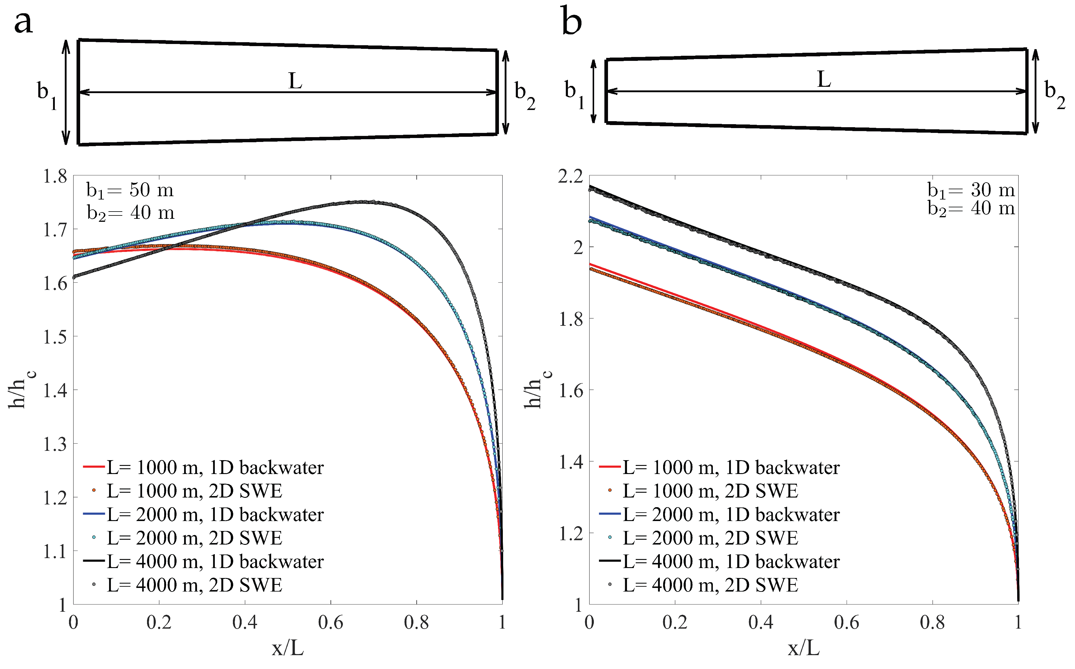
2.3. Model Verification Using Subcritical Flow: Simple Backwater Curves in Expanding/Contracting Channels

To test the hydraulic consistency of the 1D and 2D models, we present two verification cases. In the first one, we compare the water surface profiles for steady-state flow in expanding/contracting channels (Figure 2). We simulate flow in channels of different lengths whose widths vary between $b_1=50$ m and $b_2=40$ m (contracting channel, Figure 2a), and between $b_1=30$ m and $b_2=40$ m (expanding channel, Figure 2b). The discharge is $Q=500$ m${}^3$/s, the constant channel slope is $S=0.002$, and the Manning coefficient is $n=0.04$. We consider channels of increasing length, $L=1000,2000$ and 4000 m.

The construction of water surface profiles using the 1D energy-momentum theory begins with the identification of the overall hydraulic controls, which are determined by channel geometry, flow rate and bed friction properties. Our channel operates under mild slope conditions for the considered slope and total discharge: the normal depth, $h_0$, is larger than the critical depth, $h_c={\left(\frac{Q^2}{g{b}^2}\right)}^{1/3}$. The normal depth characterizes uniform flow in semi-infinite channels, so that the friction slope equals the channel slope, $S_f\left(h_0\right)=S=tan\theta$, where $S_f$ is Manning’s friction slope, defined in Equation (2). Under mild slope conditions, hydraulic control is established from the downstream boundary, where we assume free overfall conditions—we impose the critical depth, $h=h_c$. The 1D backwater profile is recovered by backwards integration of (1)–(2), with final condition $h=h_c$ (Figure 2).

For the 2D shallow-water simulations we set boundary conditions that are consistent with subcritical flow: we impose the total discharge, Q at the inlet section (flow from left to right), and critical flow conditions at the outlet. For comparison with the 1D solution, we report the water depth along the center of the channel, which matches the backwater profile (Figure 2). Note that the water surface profile is non-monotonic in the case of contracting channels (Figure 2a). In the case of 1D backwater curves, this nontrivial effect is captured through the $\partial A/\partial x$ term in Equation (1).

As a second verification test, we consider subcritical flow past a mild contraction in a long channel (Figure 3). The channel geometry is schematically represented in Figure 3a: a long channel with a total length of 6 km and width $b_1=40$ m presents a symmetric contraction, characterized by the width and length of its narrowest segment, $b_2=26.5$ m and $L_b=10$ m, respectively, and by the length of the symmetric contracting/expanding segments, $L_e$. We consider two values of this length, $L_e=100$ m (Figure 3c) and $L_e=50$ m (Figure 3d). An important geometrical parameter is the downstream distance to the free overfall boundary condition, $L_d$. We set $L_d=4000$ m, which essentially guarantees normal-depth conditions at the downstream end of the contraction. We set the distance from the upstream inlet boundary to the channel contraction as $L_u=2000$ m. The channel slope is $S=0.002$, and the we consider steady-state flow with a discharge $Q=500$ m${}^3$/s, so that the channel operates under mild slope conditions. For this flow scenario, the approaching specific energy at the downstream end of the contraction is sufficient for subcritical flow to overcome the contraction without a regime change, so that we can directly integrate the 1D backwater profile from the final condition $h=h_c$ (Figure 3b). While some 2D effects are already present in this simple exercise, a zoom-in view of the predicted water surface profiles in the contraction area shows a good match between 1D and 2D models (Figure 3c,d).

We found that the best match between the 1D and 2D profiles required the use of a slightly smaller effective Manning coefficient for the 1D simulations. Hence, we set, $n=0.04$ in the 2D model, and $n=0.0389$ in the 1D model. The need for this effective friction coefficient to achieve consistency between the 1D and 2D models could be attributed to the spatial discretization, and to the effect of friction along the side channel walls. The latter is embedded in the 1D theory, but needs to be explicitly discretized along the boundary edges of the finite volume grid in the 2D SWE. We maintain the use of this effective Manning coefficient of $n=0.0389$ in all 1D profiles hereafter, while we set $n=0.04$ in the 2D simulations.

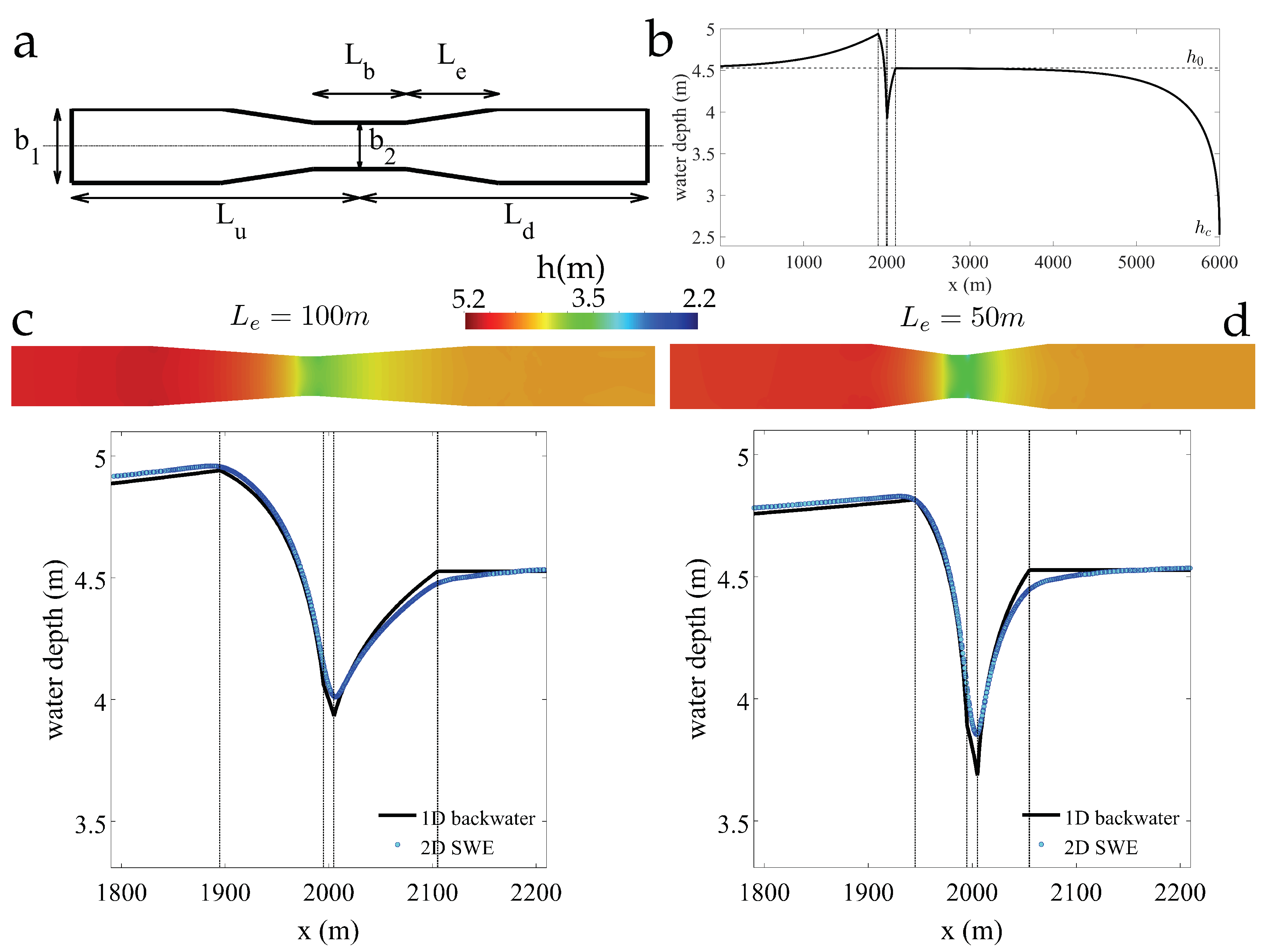
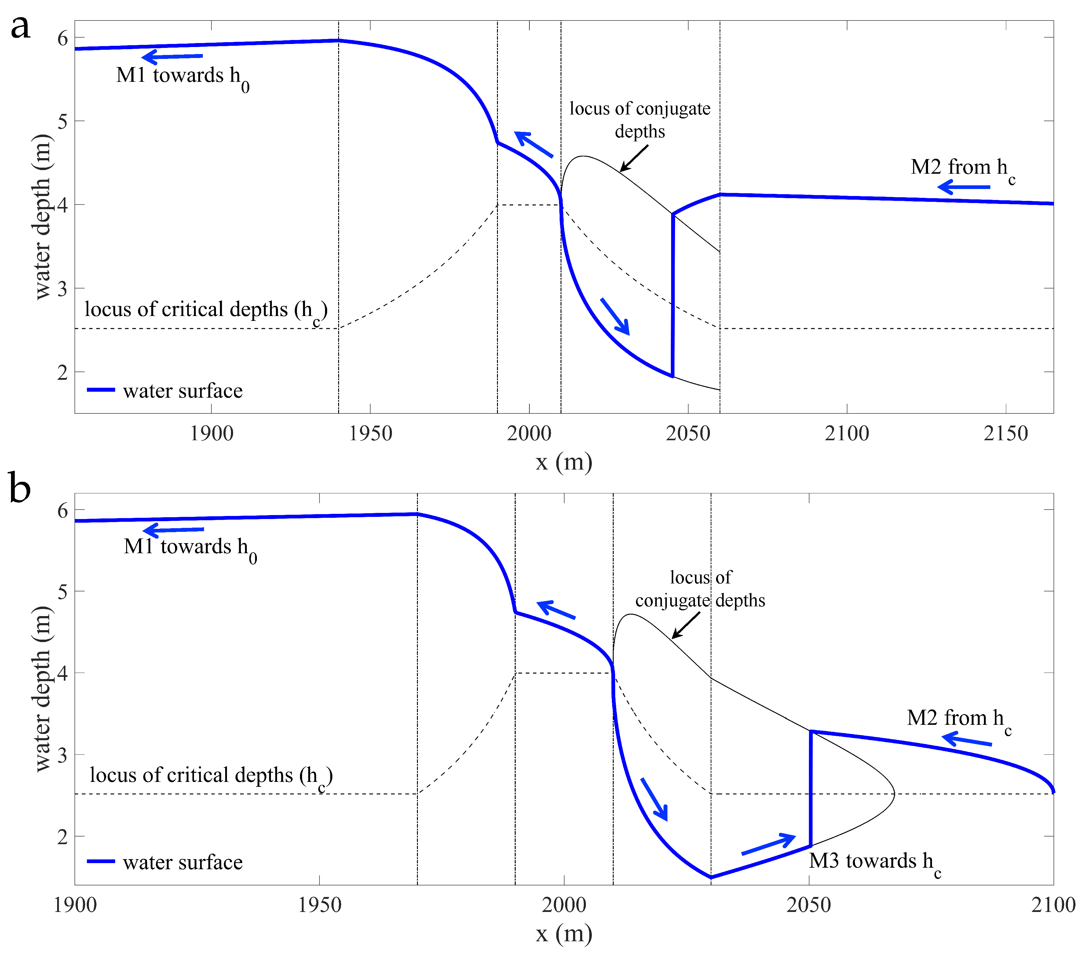
2.4. Construction of Water Surface Profiles for Transcritical Flow past a Contraction

We briefly discuss the energy–momentum method used to construct the water profiles for transcritical flow (Figure 4). As in the verification cases of Section 2.3, we consider slopes, discharges and friction parameters for which the channel operates under mild slope conditions: the overall hydraulic control is exerted from downstream to upstream sections, and undisturbed flow is subcritical. Geometrically, we consider long channels where the total discharge is known, and with free overfall conditions at the outlet (as in the examples in Figure 3). For hydraulically long channels, where the contraction is sufficiently far form the outlet, the water surface reaches the contraction with uniform depth, $h_0$. For finite, hydraulically short channels, the specific energy and depth at the downstream end of the contraction are determined by upstream integration of (1)–(2), with final condition $h=h_c$ (Figure 4). The resulting backwater curve approaches $h_0$ asymptotically from the critical depth—it is an M2 profile.

If the specific energy, as determined by the M2 backwater profile, is sufficient to overcome the contraction, the flow remains subcritical along the channel, and we may continue integrating the M2 curve upstream (e.g., the second verification problem in Section 2.3). In the absence of head losses at the channel contraction, subcritical flow requires the approaching energy to be larger than the critical energy at the narrowest section of the channel. Otherwise, the specific energy is insufficient to maintain subcritical conditions, indicating that the channel contraction induces a transition to supercritical flow. Since we consider friction losses inside the contraction, as well as the effect of a variable cross section, a direct comparison of specific energies is not a valid test for regime change. Instead, transcritical flow is revealed by the M2 profile crossing a singular point—falling below the local critical depth—as we integrate upstream along the contraction.

To reconstruct the water profile in transcritical scenarios, we begin by identifying the control section inside the channel contraction; that is, the upstream-most section where critical depth is observed. In the present case, the control section corresponds to the downstream edge of the narrowest segment of the contraction (Figure 4). Hydraulic control dictates that we must integrate (1)–(2) forward, with initial condition $h=h_c$, ending at a hydraulic jump to the approaching M2 profile. We distinguish between the case in which the jump remains in the expansion zone (Figure 4a), and the lower-energy case in which the jump is expelled out of the channel constriction (Figure 4b). In either case the location of the hydraulic jump is identified as the intersection between the specific momentum functions of the M3 and M2 curves. The physical length and complex internal structure of the jump are neglected [64], so for a rectangular channel the location is at the unique point where the depth of the approaching M2 profile, $h_{\mathrm{M}2}$ equals the conjugate of the upstream depth, $h_{u,\mathrm{conj}}$. We use the hydraulic jump formula for rectangular channels:

$$h_{u,\mathrm{conj}}=\frac{h_u}{2}\left(\sqrt{1+8{\mathrm{Fr}}_u^2}-1\right),$$

(8)

where ${\mathrm{Fr}}_u$ is the Froude number computed with the upstream depth $h_u$. Upstream from the critical section the hydraulic control reverts to being exercised from downstream sections. Hence, the water profile is constructed through backwards integration of (1)–(2), with final condition $h=h_c$. Upstream from the initial edge of the constriction we may observe either M1 or M2 profiles, depending on whether the normal depth is asymptotically approached from above or from below.

3. Results: Model Validation Using Supercritical and Transcritical Flow in Laboratory-Scale Flumes

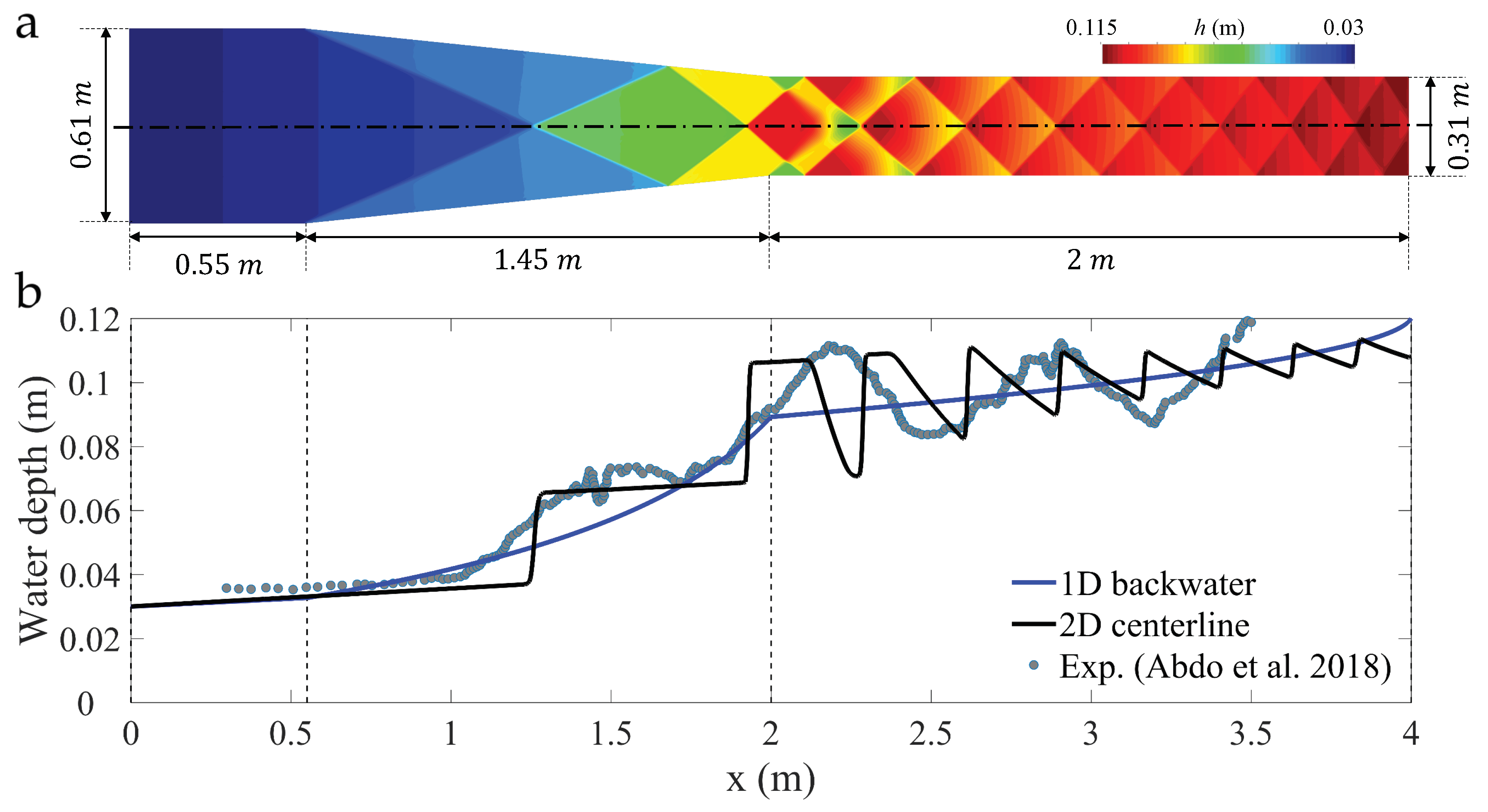
3.1. Supercritical Flow Past a Channel Contraction

In this section we consider the experimental set-up proposed by Ippen and Dawson [16], which has been used as a benchmark for models of high-velocity open channel flow over the past few decades [32,41,42,44]. The flume geometry and basic flow features (illustrated by the steady-state water depth predicted by the 2D SWE) are shown in Figure 5a. The total channel length is 4 m, with a 1.45 m contraction of 6${}^{\circ }$. The discharge is $Q=0.041$ m${}^3$/s, and the water depth at the inlet is 0.03 m, which yields a Froude number Fr≈ 4 at the inlet. The flow remains supercritical at the outlet section.

In Figure 5b we show the comparison between the recent experimental observations of [44] and our 1D and 2D model predictions. For the 1D computations we construct the 1D water profile by integrating Equations (1) and (2) forward from the inlet section, with initial condition $h=0.03$ m. For the 2D SWE, we impose supercritical inlet boundary conditions based on the known depth and total discharge, $Q=0.041$ m${}^3$/s, and supercritical flow at the outlet. Bottom friction plays an important role in this supercritical flow scenario. In Figure 5 we used a Manning coefficient $n=0.013$ for the 2D model, and $n=0.01135$ for the 1D solutions. For larger values of n the 1D theory predicts a transition to subcritical flow near the outlet.

We compare the profiles of water depth along the channel centerline (Figure 5b). The 2D shallow water theory predicts a complex pattern of oblique standing waves, while the 1D theory yields gradually varied supercritical flow throughout. The experimental observations reveal a water surface that is smoother than our 2D simulations, a feature that seems to be better described by 3D simulations [44]. Qualitatively, both the 1D and 2D models capture the overall water surface profile along the centerline.

The behavior of the water surface in this supercritical flow scenario is quite sensitive to bottom friction. Figure 6 shows the 1D and 2D predictions using several values of the Manning coefficient ($n=0.011,0.01,0.0075$ and $0.005$). Note that the experiments were conducted in a Plexiglass flume [44], for which $n\sim 0.01$ seems appropriate. Small values of the friction coefficient lead to a nearly constant water depths downstream of the contraction, which are significantly smaller than the observed ones.

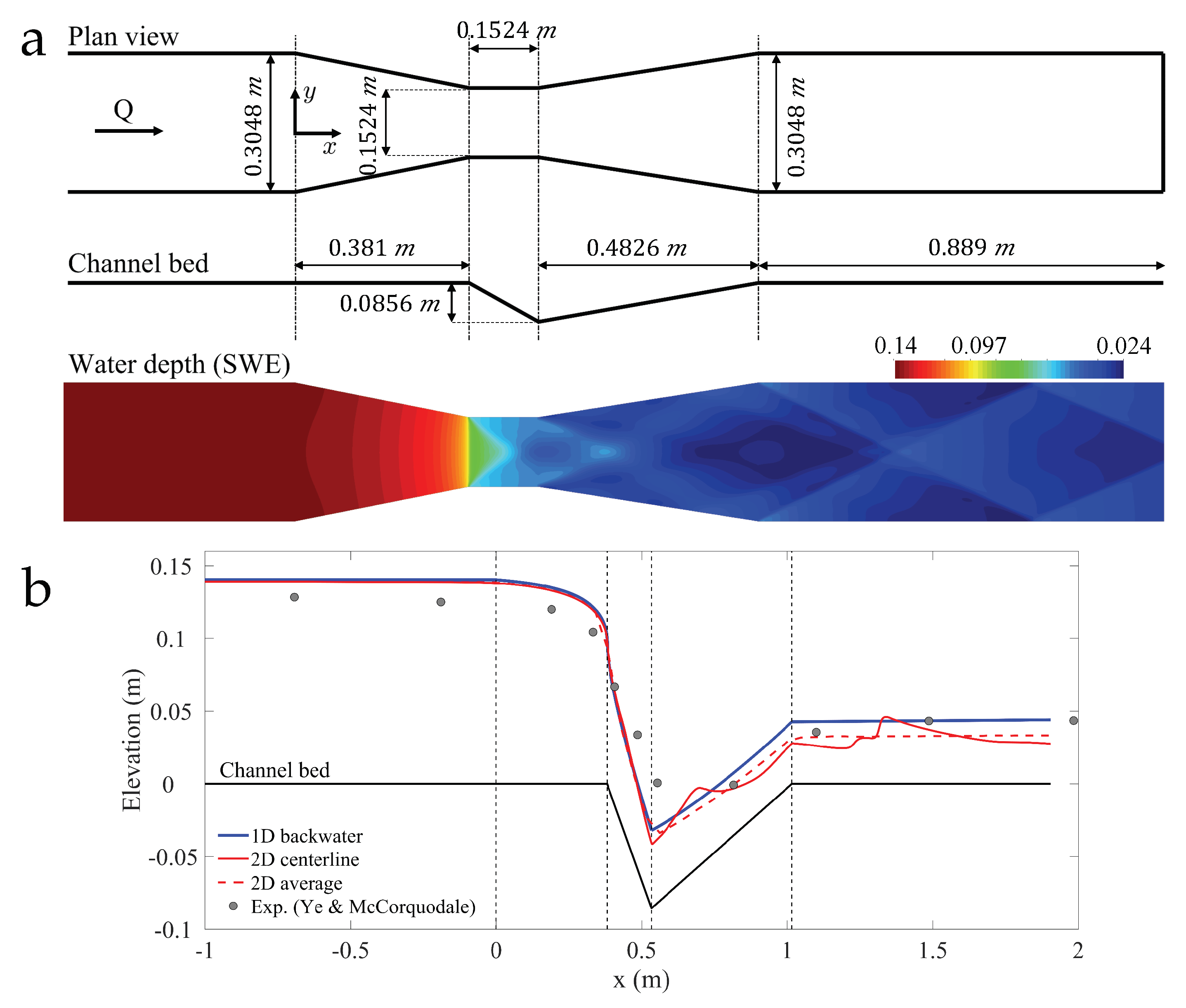
3.2. Gradually Varied Transcritical Flow in a Parshall Flume

To validate the 1D and 2D models in nontrivial cases of gradually varied flow, we consider the experiments of [43], conducted in a Parshall flume model. The problem geometry and basic flow features (illustrated by the steady-state water depth predicted by the 2D SWE) are shown in Figure 7a. The flow discharge is $Q=0.0145$ m${}^3$/s, and we set a small Manning coefficient, $n=0.005$, consistent with smooth experimental surfaces. This experimental dataset has been previously used to validate 2D shallow-water models [43] and one-dimensional, higher order theories of free surface flow that incorporate non-hydrostatic pressure effects [45]. For sufficiently refined grids, a characteristic pattern of cross-waves emerges in the supercritical region downstream of the throat (Figure 7a). The flume is short enough so that the hydraulic jump is repelled outside of the domain and the flow remains supercritical at the outlet.

For the 1D computations, the control section appears at the upstream edge of the break in slope, $x=0.381$ m. We construct the 1D water profile by integrating Equations (1) and (2) forward and backward from the control section, with initial condition $h=h_c\mp ϵ$, where $ϵ$ denotes a small perturbation introduced to avoid the singularity at the critical depth. The critical depth at the narrowest throat section is $h_c(b_1=0.1524)=0.0974$ m. For the 2D SWE, we impose subcritical inlet boundary conditions based on the known total discharge, Q, and supercritical discharge at the outlet. We find good overall agreement between the 1D and 2D predictions of water surface profile, as well as between models and experimental observations (Figure 7b). Models and experiments deviate more significantly inside the throat section and upstream from it, which we attribute to the assumption of hydrostatic pressure [45].

To test whether the discrepancy between simulations and experiments is indeed due to model assumptions rather than to grid refinement, we compare the water surface profiles along the center of the channel for various refinement levels in the 2D SWE models (Figure 8). The differences among simulation results are smaller than those between simulations and experiments, which suggests that the latter are due to the simplifications inherent to the depth-averaged shallow water theory.

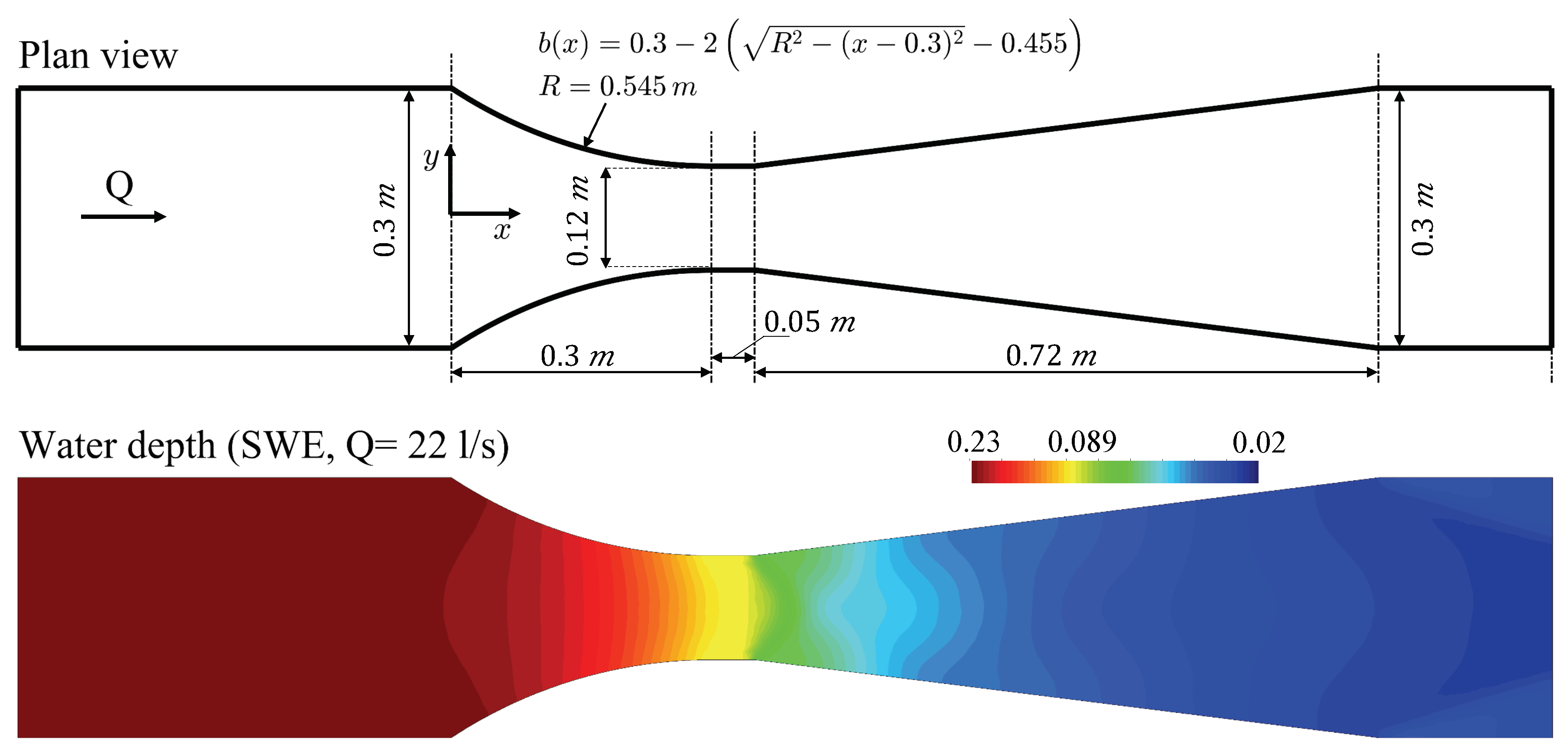
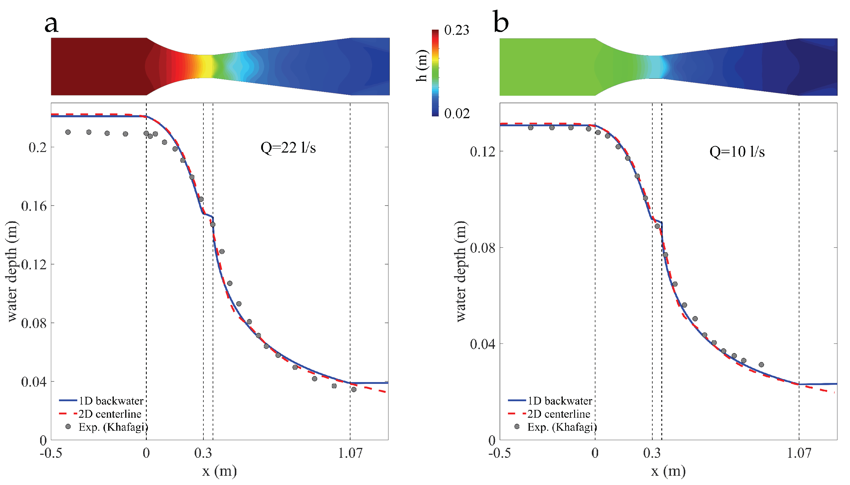
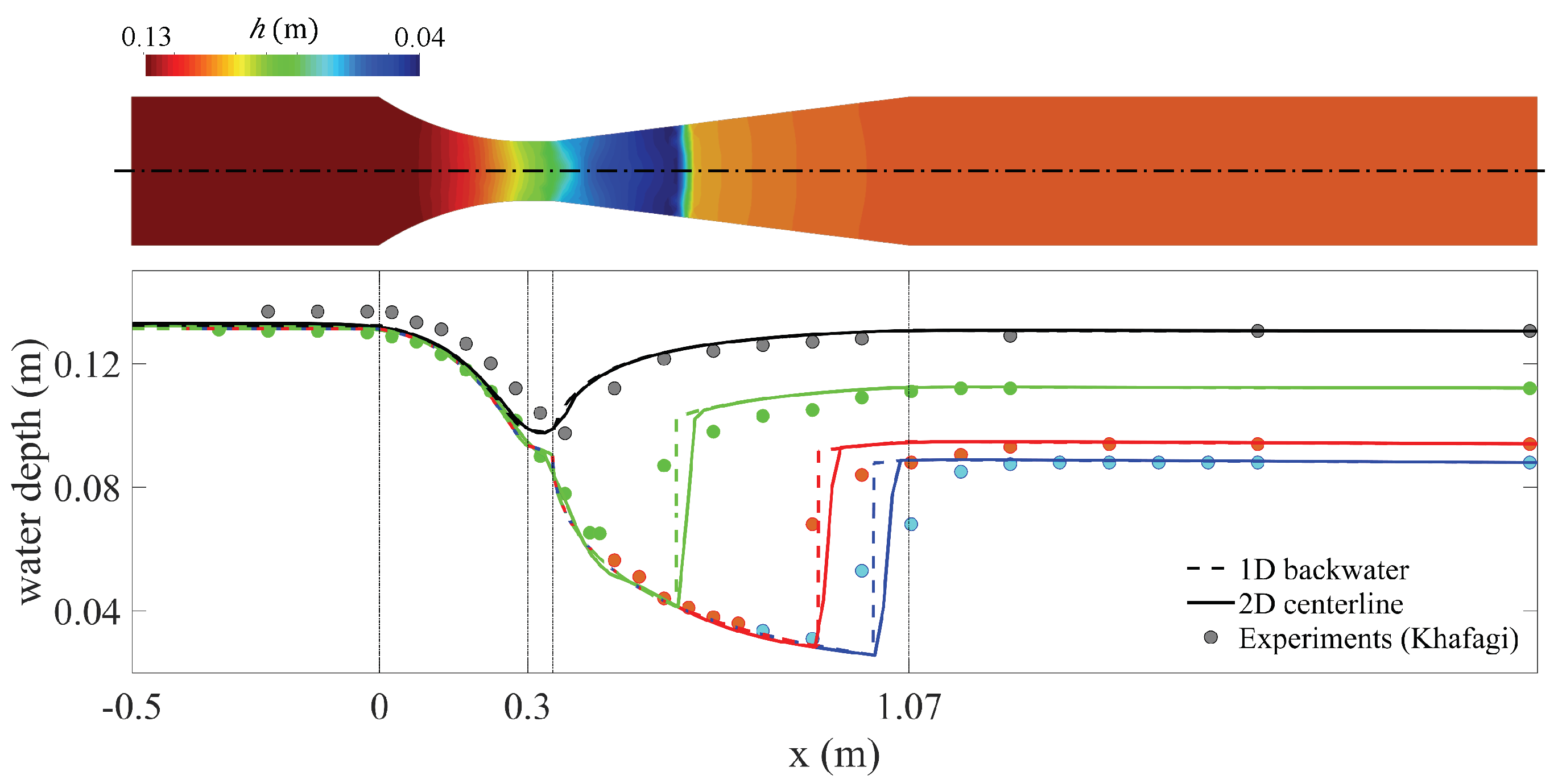
3.3. Gradually Varied Transcritical Flow in a Khafagi Flume

As a second validation case for gradually varied transcritical flows, we test model predictions against laboratory data for the classical experiments of Khafagi [24], which have been previously used to evaluate one-dimensional theories of free surface flow [45,51,52,54]. The problem geometry and basic flow features (illustrated by the steady-state water depth predicted by the 2D SWE) are shown in Figure 9. The Khafagi Venturi flume is horizontal, with a smooth converging section, a short contracted throat, and a linear diffuser with relatively small expansion rate (1/8). For this validation we consider a flume that is short enough for the hydraulic jump to be repelled out of the domain, so that flow is supercritical at the outlet and the 1D equation of gradually varied flow is applied throughout the domain. The control section appears at the upstream end of the linear expansion, $x=0.35$ m, and we construct the 1D water profile by integrating Equations (1) and (2) forward and backward from that section. For the 2D SWE we impose subcritical flow at the inlet (known total discharge Q) and critical/supercritical flow at the outlet.

We compare data and model predictions for two discharges ($Q=22$ L/s and $Q=10$ L/s), and find good overall agreement between models and experiments (Figure 10). The largest discrepancy appears in the upstream subcritical region for the $Q=22$ L/s discharge, where both 1D and 2D models predict larger water depths, which is consistent with previous calculations [52]. This deviation could be attributed to non-hydrostatic pressure effects, as 1D theories that include them show a better agreement with experimental data [45]. As in the Parshall flume model, we find very good agreement between 1D and 2D models.

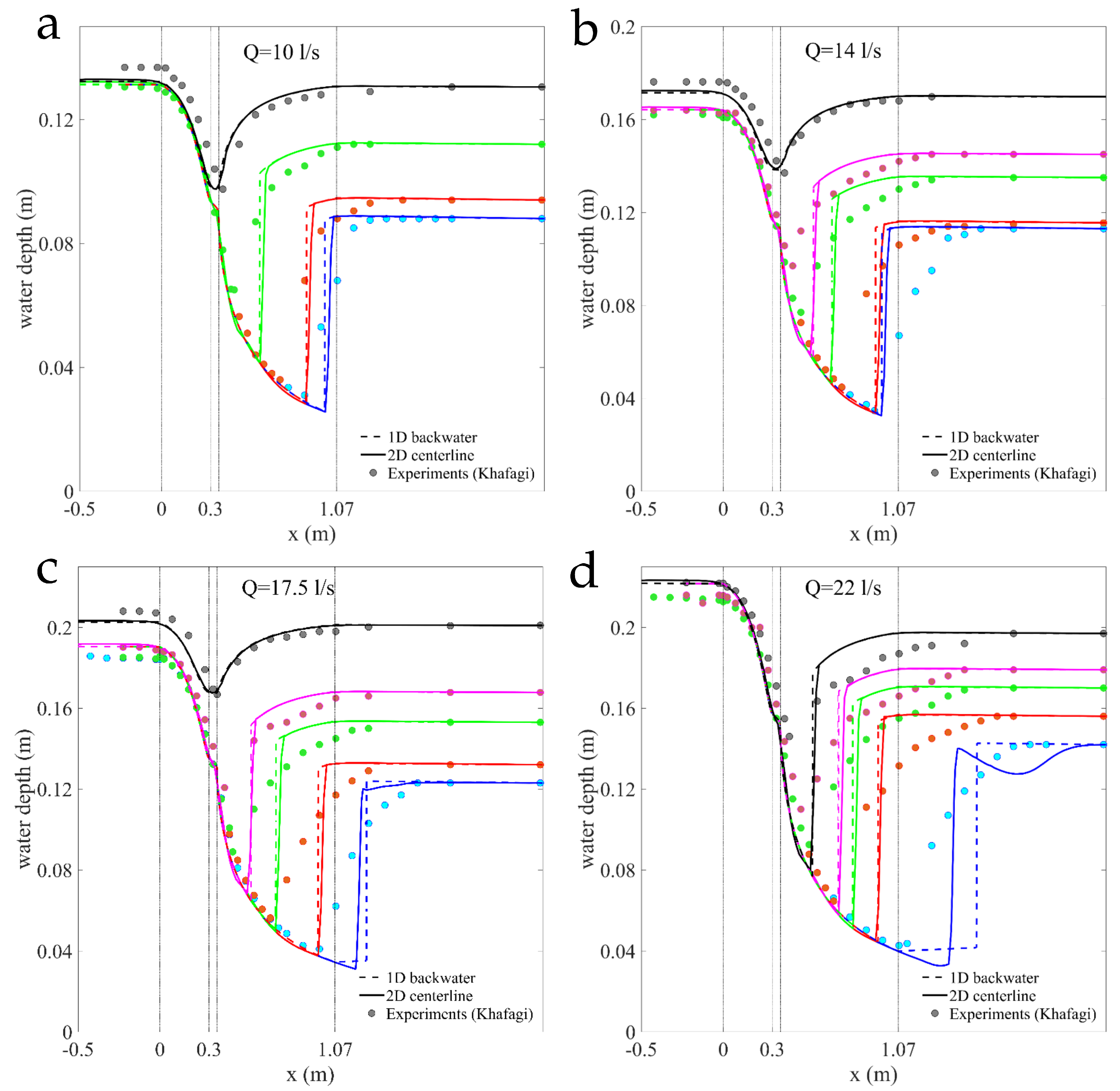
3.4. Predicting the Hydraulic Jump Position in the Khafagi’s Venturi Flume Experiments

In this section we consider a longer channel and use Khafagi’s full dataset [24]. We aim at validating the ability of the 1D classical theory and 2D SWE to capture the location of the hydraulic jump depending on the imposed tailwater depth at the downstream outlet section (Figure 11). We extend the domain to $-0.5$ m $\le x\le 2.34$ m and, while friction losses seem small in this short channel, we set a Manning coefficient of $n=0.009$ to match the position of the hydraulic jump for the lower tailwater levels. Hydraulic jumps in horizontal channels are known to be unstable with respect to their longitudinal position [54], so we use bed friction both as a stabilization mechanism and as fitting parameter. Note that we use the same value of $n=0.009$ for all discharges and tailwater depths.

We interpret Khafagi’s water surface data as including the surface roller zone above the main flow zone in hydraulic jumps. Neither the 1D classical theory nor the 2D SWE incorporate the dissipation mechanisms needed to capture the internal structure of the surface roller, so that the jump length and the details of the water profile across the jump are only approximate in the models. In fact, both depth-integrated models describe hydraulic jumps as shocks, with a simple diffusive internal structure in the case of the SWE. Some authors have proposed extended descriptions of the hydraulic jump that incorporate the separation zone and full water profile, in the spirit of [65], but such discussion falls beyond the scope of our study.

We compare the water surface profiles predicted by the models with the experimental observations, and find good overall agreement (Figure 12). We show the comparison for the four discharge values considered by Khafagi: $Q=10$ L/s, (Figure 12a), $Q=14$ L/s, (Figure 12b), $Q=17.5$ L/s, (Figure 12c), $Q=22$ L/s, (Figure 12d). For each Q, the transition from free overfall to fully subcritical conditions is characterized by a sequence of increasing tailwater depths: $h_d=0.0880,0.0940,0.1120,$ and $0.1305$ m (for $Q=10$ L/s); $h_d=0.1130,0.1155,0.1350,0.1450,$ and $0.1698$ m (for $Q=14$ L/s); $h_d=0.1230,0.1320,0.1530,0.1678,$ and $0.2010$ m (for $Q=17.5$ L/s); $h_d=0.1420,0.1560,0.1700,0.1790,$ and $0.1970$ m (for $Q=22$ L/s).

The jump location predicted by the models is remarkably accurate, given the uncertainty due to the representation of hydraulic jumps as shock fronts. The discrepancy between models and experiments increases with flow discharge, which may be attributed to a more complex internal structure of hydraulic jumps as the Froude number increases. The overall conclusion drawn from the experimental validation exercise is that the 1D and 2D models predict very similar water surface profiles and jump positions for transcritical flow past short, horizontal channels with relatively smooth contractions and without significant flow separation. The deviations between models and experiments may lie in the limitations of the depth-averaged theories, in particular the non-hydrostatic nature of the pressure, and the impact of streamline curvature [45,46,51,54].

4. Results: Transcritical Flow in Long Channels

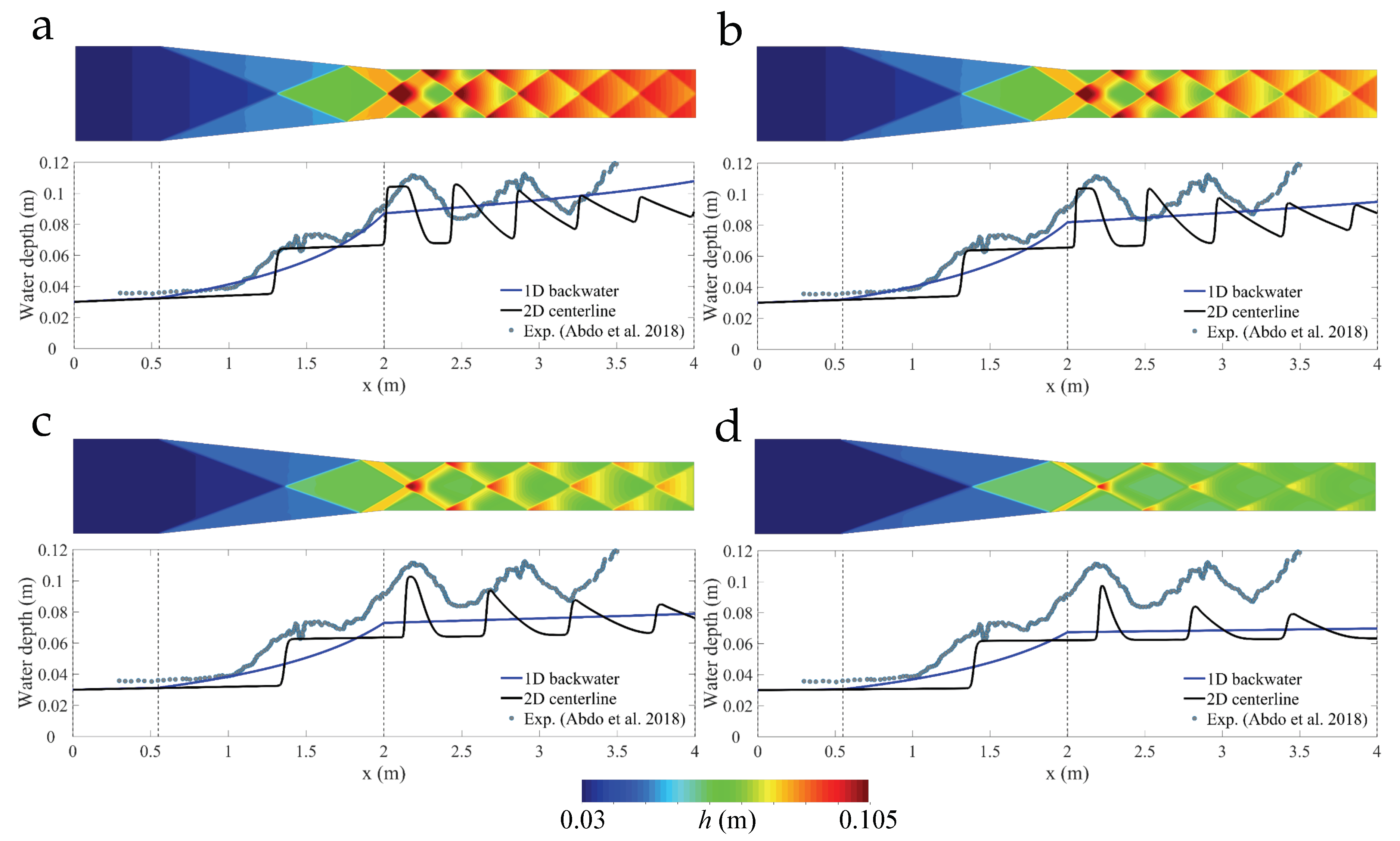
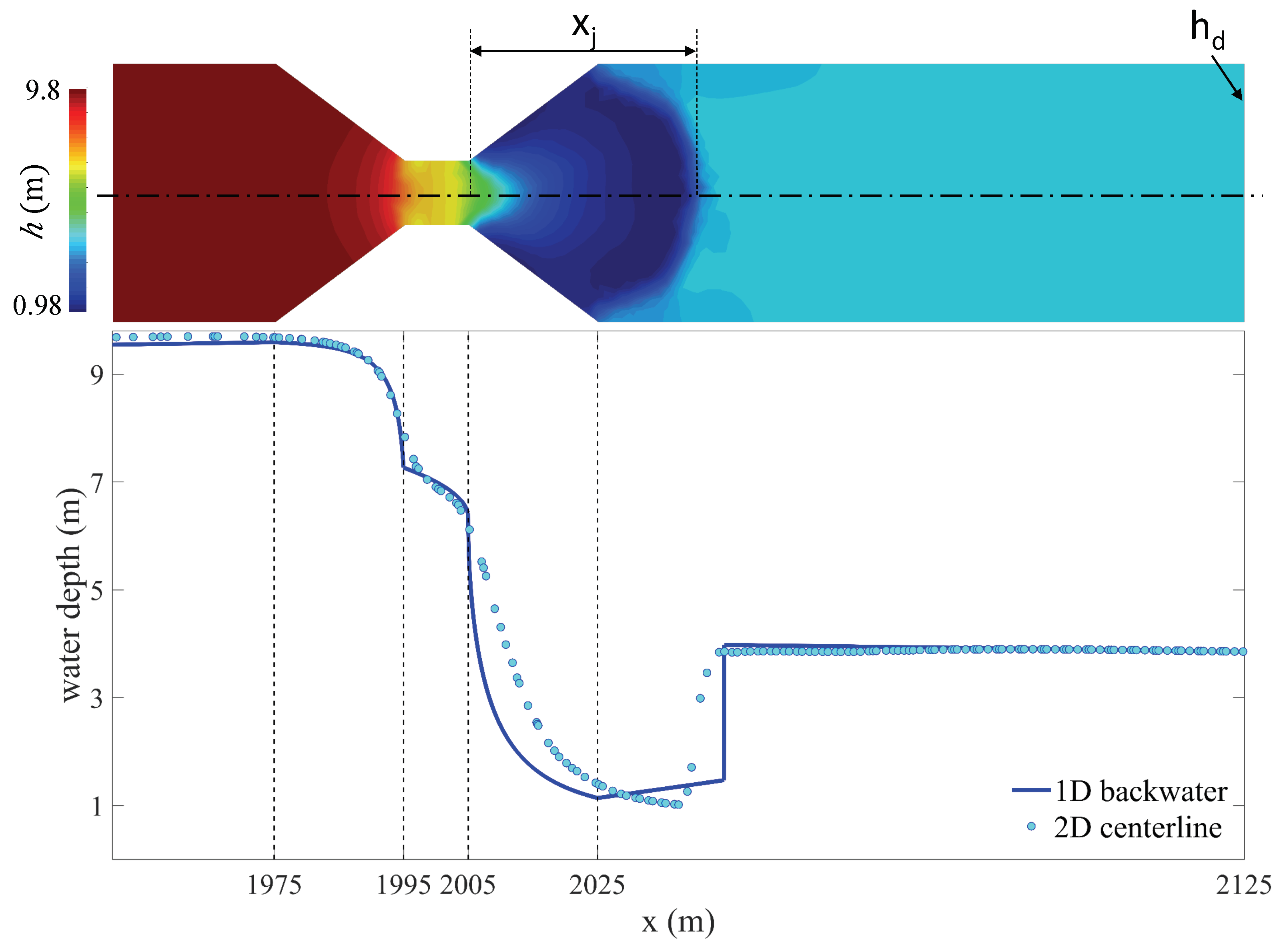
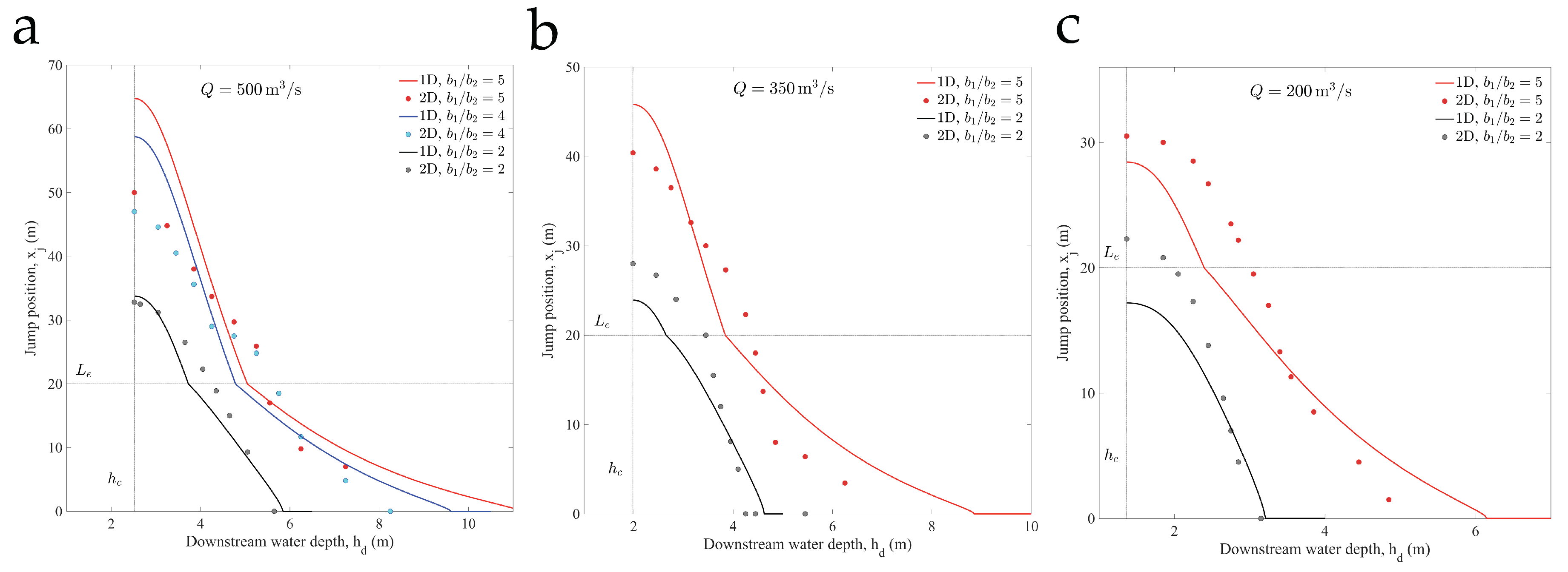
4.1. Predicting the Onset of Transcritical Flow and Jump Position in a Long Channel with a Linear Contraction

An important practical question is whether the simplified 1D theory can be used to predict the transition from fully subcritical flow to mixed-regime flow, where a repelled hydraulic jump appears downstream of the contracted section. A correct description of such transition requires a model that can capture the influence of downstream energy conditions, through an imposed tailwater level or the effect of a backwater curve, on the specific energy and momentum transfer induced by the contraction.

We quantitatively compare the predictions of the 1D and 2D models in the case of a long channel, where the available specific energy at the contraction is controlled by the tailwater depth at the outlet, and by a relatively short backwater curve that develops upstream (Figure 13 and Figure 14). We use the basic channel geometry shown in Figure 3a, with approach flow width $b_1=40$ m and a symmetric, linear contraction that reduces the width to a minimum value $b_2$ over a distance $L_e=20$ m. This minimum width remains constant over a throat section of length $L_b=10$ m. The Manning coefficient is $n=0.04$ and the geometric slope is $S_0=0.002$. The distance to the outlet is short enough ($L_d=125$ m) so that the boundary condition is essentially maintained as the tailwater depth of the jump. We solve steady-state flow for several values of the discharge, Q, throat width, $b_2$, and imposed tailwater depth, $h_d$. For each parameter combination, we determine the location of the hydraulic jump, $x_j$, using the 1D theory and the 2D shallow-water Equations (Figure 13). For the shallow-water simulations, we report the position of the jump based on the water depth profile along the axis of the channel.

We consider three flow discharges, $Q=500,350$ and 200 m${}^3$/s, and three width ratios, $b_1/b_2=2,4,5$, and plot the predicted jump locations, $x_j$, against the imposed tailwater depth, $h_d$ (Figure 14). Note that the jump is repelled out of the expansion zone when $x_j>L_e$, and the flow becomes fully subcritical when $x_j=0$. The maximum value of $x_j$ corresponds to free overfall conditions, for which the imposed depth at the outlet equals the critical depth for each value of the discharge. The 1D theory overpredicts the distance to the hydraulic jump for large tailwater depths, as well as the threshold tailwater depth for which flow becomes subcritical ($x_j=0$, Figure 14). It is interesting that the situation reverses for small tailwater depths, for which the jump is repelled outside of the expansion zone, at the lower discharge ($Q=200$ m${}^3$/s, Figure 14c). The discrepancy between 1D and 2D predictions can be explained in part by the fact that we report distance along the channel axis in the 2D simulations.

To test a more realistic outlet boundary condition, we compare the 1D and 2D model predictions for a milder contraction, $b_2=26.5$ m, same length of the converging/expanding sections, $L_e=20$ m, discharge $Q=500$ m${}^3$/s, and several values of the distance to the outlet, $L_d$, where we imposed free overfall conditions. For this long channel, friction losses are large enough so that the available specific energy at the contraction is controlled by a backwater curve starting from the critical depth at the outlet. We induce the onset of transcritical flow at the throat section by reducing the distance to the outlet, $L_d$ (Figure 15). Both 1D and 2D models predict near-critical flow conditions for hydraulically long channels, $L_d=4000,500$ m, and the onset of repelled hydraulic jumps (R-jumps) [26,28] for the shorter distances, $L_d=250,125$ m (Figure 15d). The development of the backwater profile leads to a flow pattern downstream of the contraction that is more complex than in the case of a short channel with imposed tailwater depth. The relatively abrupt expansion induces flow separation at the downstream edge of the throat, which may prevent the 2D SWE from reaching a true steady state flow solution due to a vortex shedding instability (Figure 15a). A comparison of the water surface profiles predicted by the 1D and 2D models (the latter along the channel axis) suggests that spatial flow structures delay the transition in 2D simulations, relative to the strict 1D theory, where a sharp hydraulic jump appears as soon as the available energy is insufficient to overcome the channel contraction (Figure 15d). For distances to the outlet that are short enough for R-jumps to appear in the 2D model (Figure 15d), the 1D theory performs reasonably well at predicting the location of the jump, but not the gradually varied water surface profile leading to the toe of the jump (Figure 15d, $L_d=250$ m). If the specific energy is further reduced, larger Froude number conditions lead to flow patterns dominated by oblique shocks that render the 1D analysis invalid in the expansion zone (Figure 15, panels c and d, $L_d=250$ m).

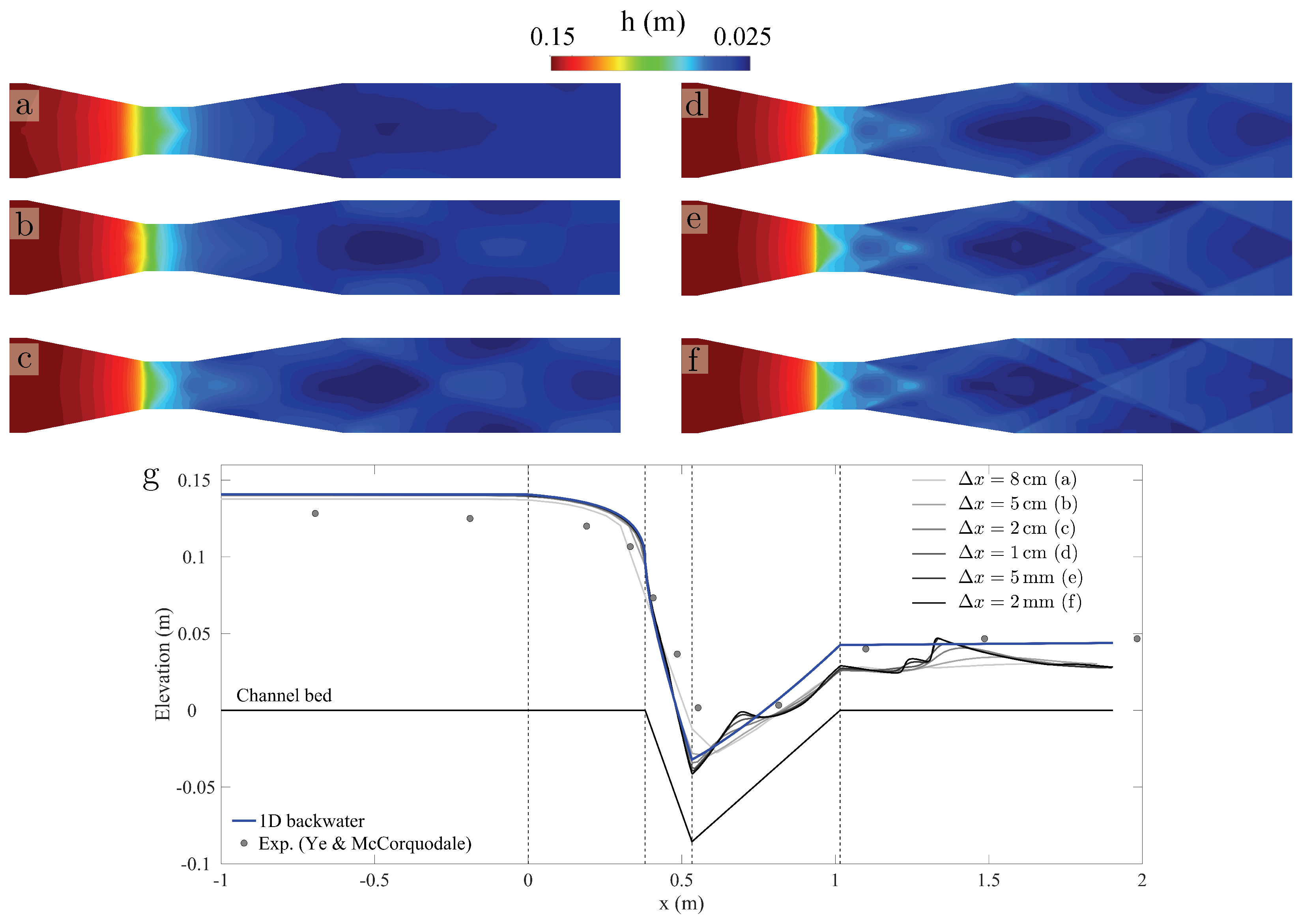
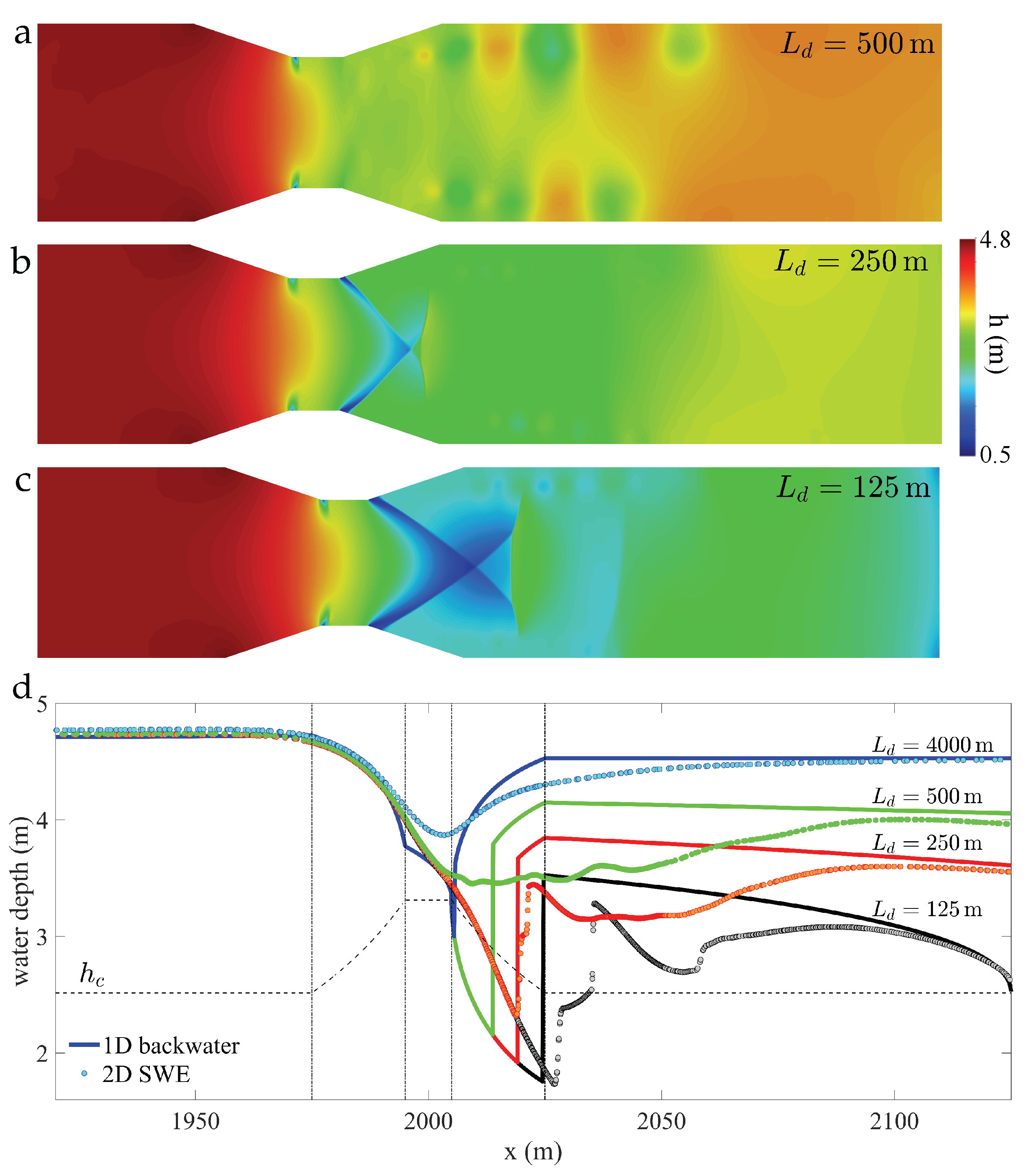
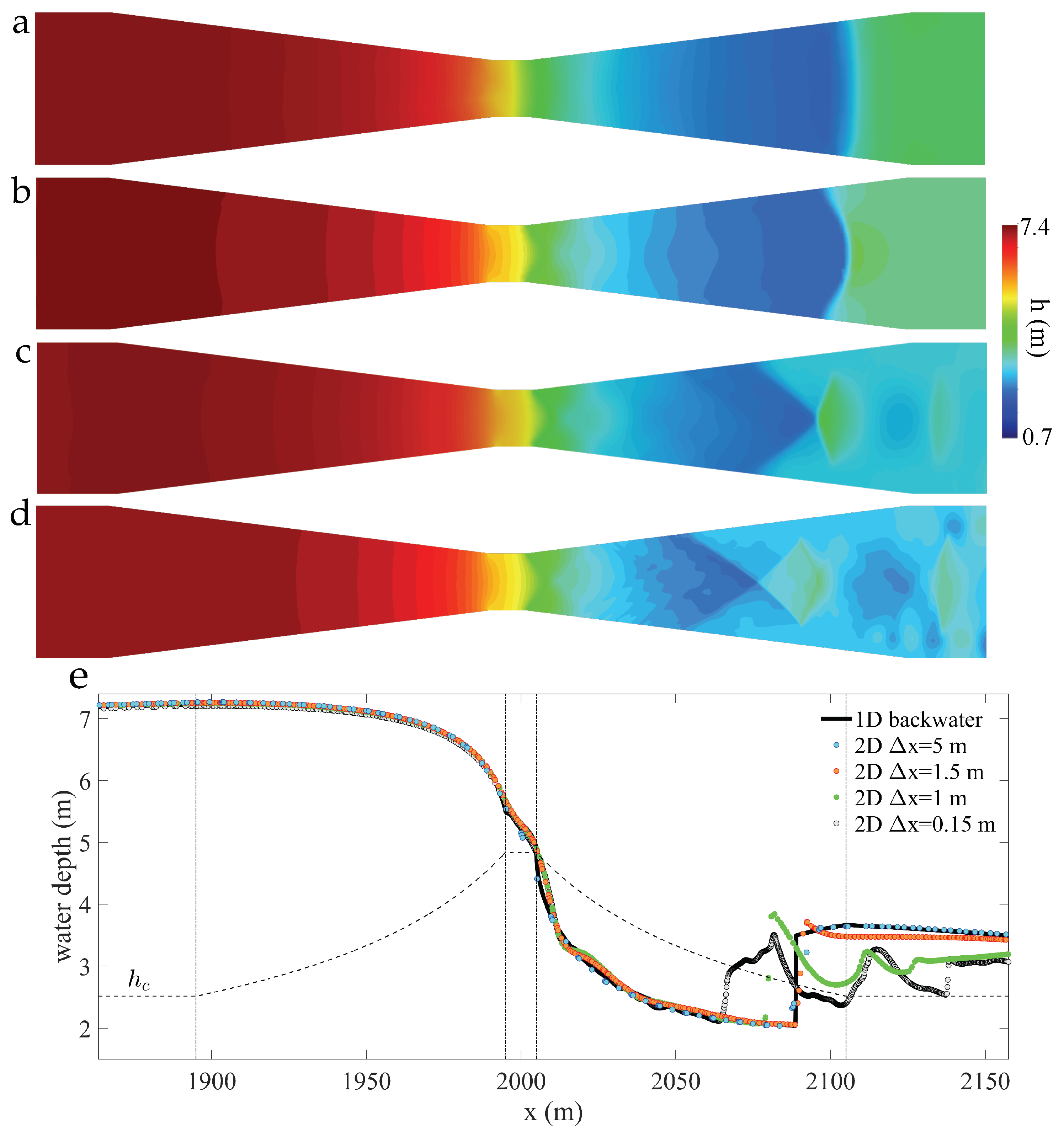
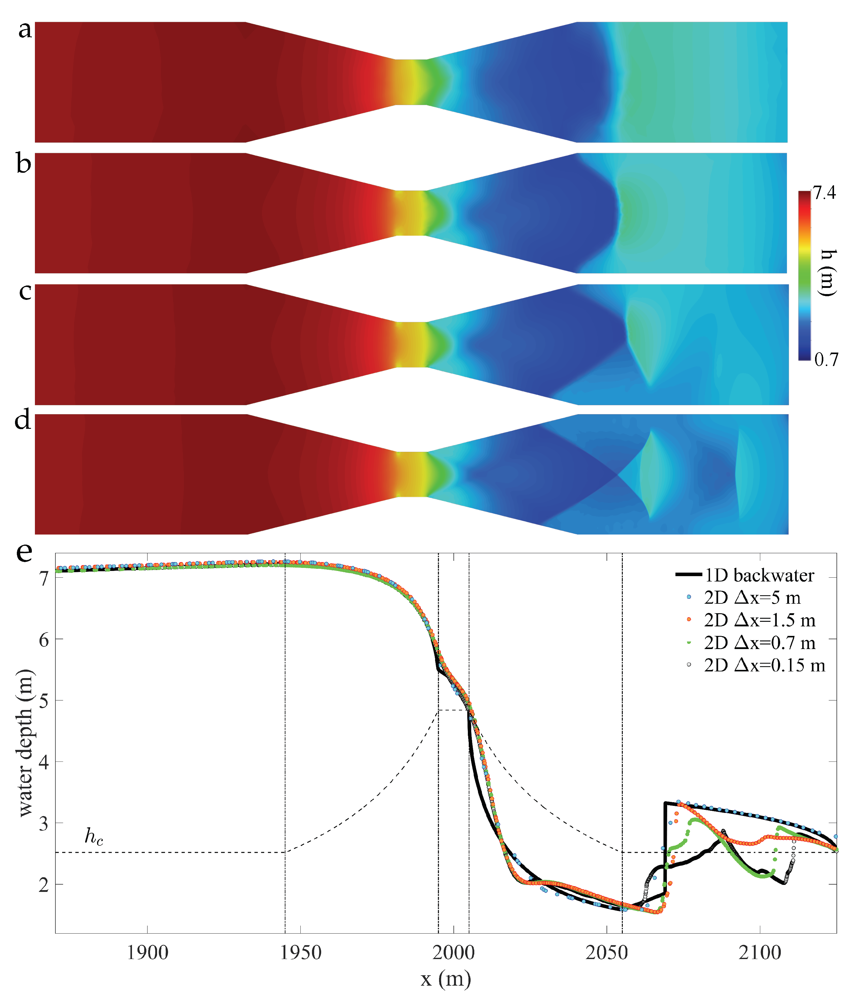
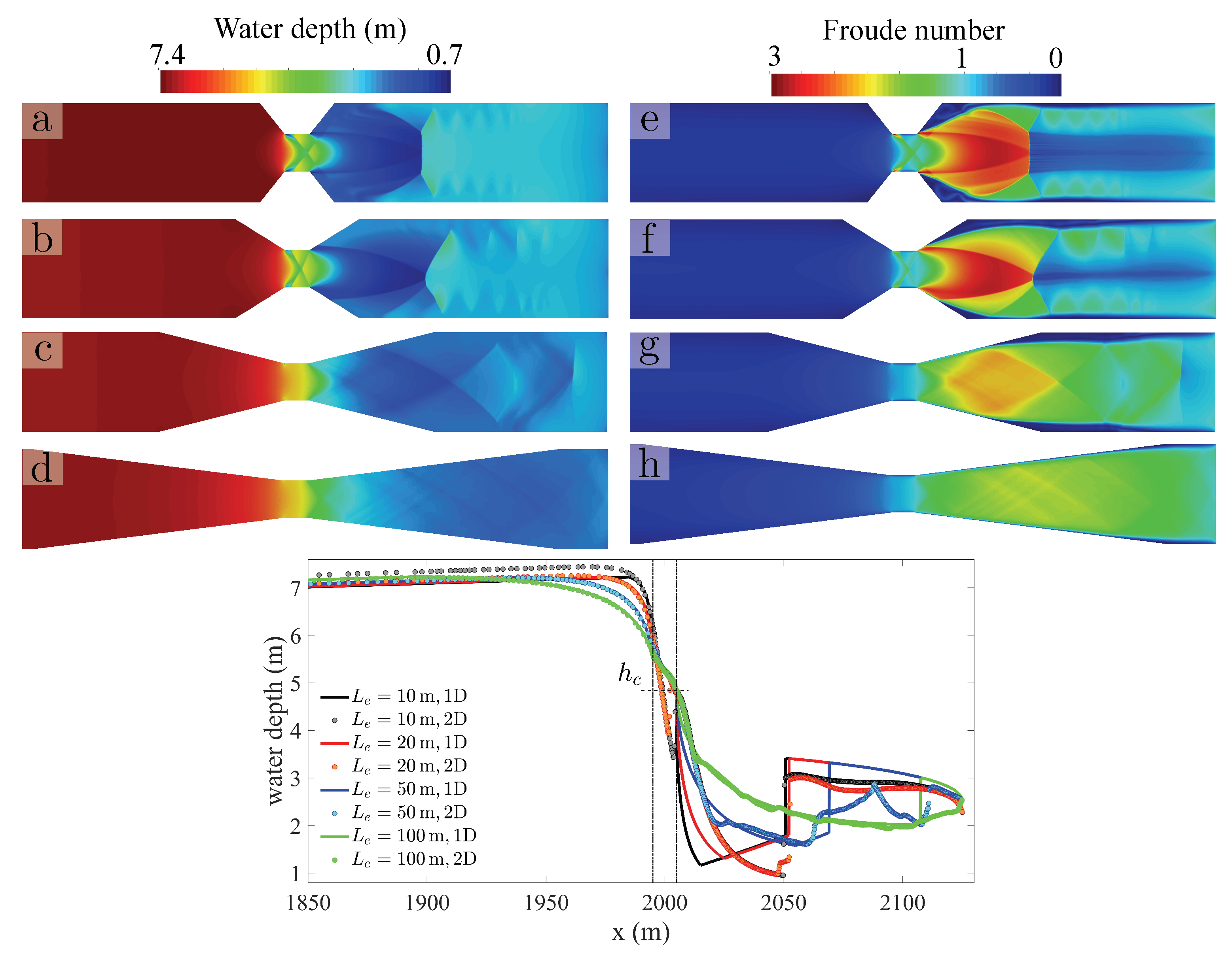
4.2. The Role of Grid Refinement on Capturing 2D Flow Features

Hydrodynamic simulations in long river sections and channels often rely on the available topography data, whose spatial resolution is typically 1–5 m. Even if higher-resolution bathymetry were available, affordable grids in kilometer-long channels may be limited to meter-scale resolutions, which implies ≈10–20 grid cells across the channel width. We study the impact of grid resolution on the simulated flow patterns, and on the differences between 1D and 2D predictions, by performing a refinement study on two transcritical scenarios (Figure 16 and Figure 17). Some of the model parameters are common to both cases: $b_1=40$ m, $b_2=15$ m, $Q=500$ m${}^3$/s, and $n=0.04$, with the channel geometry of Figure 3a. By changing the length of the contraction/expansion segment, $L_e$, and the distance to outlet, $L_d$, we explore the two scenarios described in Figure 4: one with the hydraulic jump contained inside the expansion zone ($L_e=100$ m, $L_d=250$ m, Figure 16), and another one with the jump expelled outside of the expansion zone ($L_e=50$ m, $L_d=125$ m, Figure 17).

We consider four refinement levels: a very coarse mesh, with a typical grid size $\Delta x=5$ m in the channel contraction, which implies three grid cells across the narrowest section (Figure 16a and Figure 17a); a very fine mesh, with a typical grid size $\Delta x=0.15$ m in the channel contraction, which implies 100 grid cells across the narrowest section and over 400 K control volumes in total (Figure 16d and Figure 17d); and two intermediate refinement levels, with typical grid sizes $\Delta x=1.5$ m and $\Delta x=1$ m in the channel contraction (Figure 16b,c and Figure 17b,c).

The water depth profiles along the axis of the channel (for the 2D models) agree with the water surface constructed using the 1D theory (Figure 16a–e and Figure 17a–e). This is because corse-grid 2D simulations do not capture the spatial flow effects induced by the contraction, rendering the simulations quasi-1D ones. As the grid is refined, a complex structure dominated by oblique standing waves emerges in the fine-grid 2D simulations, which strongly deviate from the 1D theory (Figure 16d–e and Figure 17d–e). Despite its limitations, it is remarkable that the simple 1D theory captures the water surface profile upstream from the critical section at the contraction, and even the overall features of the gradually varied supercritical flow region in the expansion zone. All 2D simulations hereafter have been performed using a highly refined mesh (typical grid size $\Delta x=0.15$ m in the channel contraction).

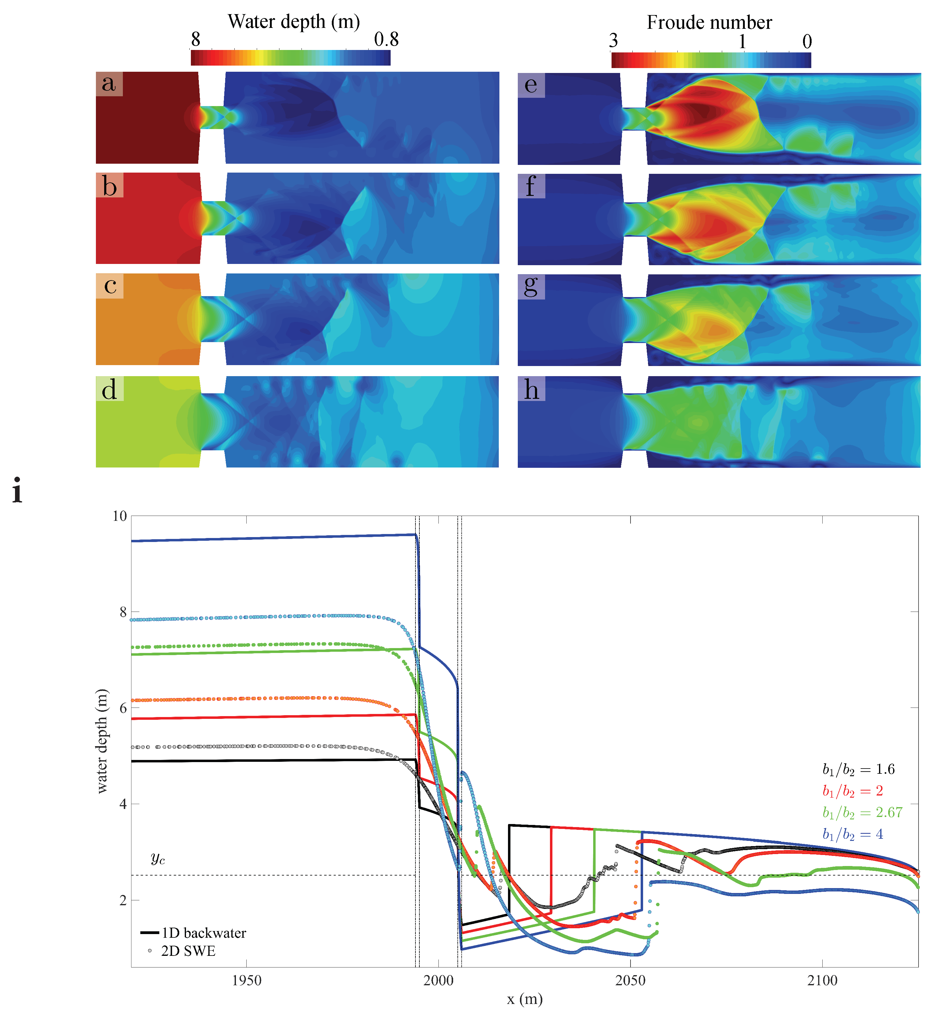
4.3. Influence of the Contraction Geometry on the Discrepancy between 1D and 2D Models

We explore the role of the contraction geometry on the spatial flow patterns and on the agreement between 1D and 2D models (Figure 18). For a smooth contraction, with $L_e=100$ m, the 1D theory captures the gradually varied flow in the expansion zone remarkably well (Figure 18d). This supercritical flow region is also well described in the $L_e=50$ m case, in spite of the complex shock interaction that ensues downstream of the expansion. Two-dimensional effects dominate the flow for the sharpest contraction ($L_e=10$ m, Figure 18a): while the location of the hydraulic jump seems to be correctly predicted by the 1D theory, the overall structure of the water surface downstream from the expansion zone is lost in the 1D model. Notably, the 2D model predicts the onset of oblique waves within the narrow, constant-width central segment of the contraction for $L_e=10$ m and $L_e=20$ m (Figure 18a,b). This fundamental deviation from the 1D analysis leads to a large discrepancy between the 1D and 2D models in the gradually varied supercritical flow region, although the location of the hydraulic jump seems to be correctly predicted by the 1D theory.

The abruptness of the expansion and contraction segments affects the Froude number in the expansion zone and downstream from it (Figure 18e–h), illustrating the strong flow-focusing effect of an abrupt change in channel width. Only the smoother geometry, $L_e=100$ m, avoids the appearance of a large region of separated flow in the expansion zone, (Figure 18h), which partially explains the more satisfactory performance of the 1D model.

The violation of the assumption of uniform flow across the channel becomes particularly clear for large width ratios, $b_1/b_2$ (Figure 19). We increase the Froude number downstream of the contraction by keeping the flow conditions of Figure 3, Figure 16 and Figure 17, and considering an abrupt contraction, $L_e=1$ m, while reducing the width of the narrowest segment ($b_1=25,20,15,$ and 10 m). The resulting Froude numbers downstream of the constriction range from near unity to over 3 (Figure 19e–h), due to the water pile-up upstream from it (Figure 19a–d). Both the complexity of the 2D patterns, and the local head losses, increase with $b_1/b_2$, as does the deviation with respect to the 1D theory (Figure 19i). These extreme cases of abrupt transition and large values of the width ratio illustrate the limitations of the 1D theory, as both the predictions of the water surface profile upstream and downstream from the contraction become incorrect (Figure 19i). It is apparent that multidimensional simulations would be required in the design of hydraulic structures with such geometrical constraints.

5. Discussion and Conclusions

Abrupt channel expansions and contractions lead to head losses that are typically modeled as localized energy losses [3,6]. Expansion losses can be significant due to flow focusing and viscous dissipation in the separated zones. While a number of expressions have been proposed to account for these losses in the context of the 1D theory [4], this type of flow patterns are a paradigmatic example of situations where well resolved multidimensional models are preferred.

The onset of oblique standing waves is a ubiquitous feature of supercritical open channel flow [3,15,16,17]. The appearance of oblique shocks fundamentally alters the momentum transfer mechanisms in the channel expansion zone, so that the underlying assumption of uniform flow used by the 1D theory no longer applies. For sharp enough contractions, another source of discrepancy between 1D and 2D predictions in the studied geometries is the emergence of oblique shocks in the constant-width narrow segment of the contraction. The 1D model assumes that the critical section is located at the downstream end of this central segment, so the structure of the water profile in the gradually-varying supercritical region is not captured correctly. The maps of Froude numbers in Figure 19, for example, show that the spatial effect of the oblique shocks also propagates downstream from the contraction, invalidating the assumption of uniform flow across the channel width made by the 1D theory.

Two-dimensional flow patterns, in particular flow detachment and oblique standing waves, control the energy and momentum transfer mechanism in open channel flow past abrupt contractions with a large width ratio. Only modified versions of the 1D theory, taking into account intense local head losses and the propagation of spatial flow structures downstream from the contraction, can succeed at describing these flow scenarios. Multidimensional calculations would be required in the design of hydraulic structures with such geometrical constraints.

In this paper we compare well resolved 2D shallow-water simulations with 1D energy-momentum calculations for transcritical flow past symmetric channel contractions. We analyze the accuracy of the classical energy-momentum gradually varied flow computations to predict the onset of regime transitions and the location of hydraulic jumps. We validated our 1D and 2D models using available data from laboratory-scale Venturi-type flumes, and test the relative performance of the simplified 1D theory for different constriction geometries, identifying the flow mechanisms behind the discrepancies between the 1D and 2D theories.

Our main conclusions can be summarized as:

• For transcritical flow past short, horizontal channels with relatively smooth contractions and negligible flow separation (e.g., for the experimental cases considered in the validation section), the deviations between models and experiments seem larger than among models. The discrepancy between models and experimental data is consistent with the well known limitations of the depth-averaged shallow-water model, in particular the impact of non-hydrostatic pressures and streamline curvature on the flow. The standard 1D theory shares this limitation.
• Considering its simplicity and negligible computational cost, the classical 1D theory performs remarkably well for a wide range of flow conditions and relatively smooth channel contractions. In particular, the 1D model yields a good prediction of the transition to supercritical flow at the contraction. Perhaps more importantly, the 1D model is more conservative, in the sense that it predicts an earlier onset of critical flow at the contraction as the tailwater depth decreases.
• The grid resolution used in the 2D SWE simulations plays an important role in capturing the spatial flow patterns, so that coarse grid 2D simulations provide essentially the same information as 1D ones. The implication of this observation is that the discrepancies among various 2D models with different spatial grid resolution may be as large as those between the 2D models and a classical 1D energy-momentum calculation. The impact of grid resolution on the agreement between 1D and 2D models is relevant in practice, as field-scale hydrodynamic models in fluvial dynamics rely on the available topography, whose spatial resolution is often limited to the meter scale.

References

1. Bakhmeteff, B.A. Hydraulics of Open Channels; McGraw-Hill: New York, NY, USA, 1932. [Google Scholar]
2. Castro-Orgaz, O.; Sturm, T.W.; Boris, A. Bakhmeteff and the Development of Specific Energy and Momentum Concepts. J. Hydraul. Eng. 2018, 144, 02518004. [Google Scholar] [CrossRef]
3. Chow, V.T. Open-Channel Hydraulics; McGraw-Hill: New York, NY, USA, 1959. [Google Scholar]
4. Henderson, F.M. Open Channel Flow; Mcmillan Publishing Co., Inc.: New York, NY, USA, 1966. [Google Scholar]
5. Chanson, H. The Hydraulics of Open Channel Flow: An Introduction, 2nd ed.; Elsevier Butterworth-Heinemann: Burlington, MA, USA, 2004. [Google Scholar]
6. Sturm, T.W. Open Channel Hydraulics; McGraw-Hill: New York, NY, USA, 2001. [Google Scholar]
7. Deltares. Simulation of Multidimensional Hydrodynamic Flows and Transport Phenomena, Including Sediments; User Manual; Deltares: Delft, The Netherlands, 2011. [Google Scholar]
8. Bladé, E.; Cea, L.; Corestein, G.; Escolano, E.; Puertas, J.; Vázquez-Cendón, E.; Dolz, J.; Coll, A. Iber: Herramienta de simulación numérica del flujo en ríos. Rev. Int. Métodos Numér. Cálc. Diseño Ing. 2014, 30, 1–10. [Google Scholar] [CrossRef]
9. Hager, W.H. Transitional Flow in Channel Junctions. J. Hydraul. Eng. 1989, 115, 243–259. [Google Scholar] [CrossRef]
10. Hager, W.H.; Castro-Orgaz, O. Transcritical Flow in Open Channel Hydraulics: From Boss to De Marchi. J. Hydraul. Eng. 2016, 142, 02515003. [Google Scholar] [CrossRef]
11. Chanson, H.; Montes, J.S. Characteristics of undular hydraulic jumps: Experimental apparatus and flow patterns. J. Hydraul. Eng. 1995, 121, 129–144. [Google Scholar] [CrossRef]
12. Montes, J.S.; Chanson, H. Characteristics of Undular Hydraulic Jumps: Experiments and Analysis. J. Hydraul. Eng. 1998, 124, 192–205. [Google Scholar] [CrossRef] [Green Version]
13. Ohtsu, I.; Yasuda, Y.; Gotoh, H. Flow Conditions of Undular Hydraulic Jumps in Horizontal Rectangular Channels. J. Hydraul. Eng. 2003, 129, 948–955. [Google Scholar] [CrossRef]
14. Bose, S.K.; Castro-Orgaz, O.; Dey, S. Free Surface Profiles of Undular Hydraulic Jumps. J. Hydraul. Eng. 2012, 138, 362–366. [Google Scholar] [CrossRef] [Green Version]
15. Ippen, A.T. High-Velocity Flow in Open Channels: A Symposium: Mechanics of Supercritical Flow. ASCE Trans. 1951, 116, 268–295. [Google Scholar]
16. Ippen, A.T.; Dawson, J.H. Design of channel contractions. ASCE Trans. 1951, 116, 326–346. [Google Scholar]
17. Ippen, A.T.; Harleman, D.R.F. Verification of Theory for Oblique Standing Waves. ASCE Trans. 1956, 121, 678–694. [Google Scholar]
18. Behlke, C.E.; Pritchett, H.D. The Design of Supercritical Channel Junctions; Highway Res. Record, Nr. 123, Publication 1365, 17-35; Highway Research Board, National Research Council: Washington, DC, USA, 1966. [Google Scholar]
19. Hager, W.H. Supercritical Flow in Channel Junctions. J. Hydraul. Eng. 1989, 115, 595–616. [Google Scholar] [CrossRef]
20. Rouse, H.; Bhoota, B.V.; Hsu, E.Y. Design of channel expansions. ASCE Trans. 1951, 116, 347–363. [Google Scholar]
21. Akers, B.; Bokhove, O. Hydraulic flow through a channel contraction: Multiple steady states. Phys. Fluids 2008, 20, 056601. [Google Scholar] [CrossRef] [Green Version]
22. Defina, A.; Viero, D.P. Open channel flow through a linear contraction. Phys. Fluids 2010, 22, 036602. [Google Scholar] [CrossRef]
23. Viero, D.P.; Defina, A. Extended Theory of Hydraulic Hysteresis in Open-Channel Flow. J. Hydraul. Eng. 2017, 143, 06017014. [Google Scholar] [CrossRef] [Green Version]
24. Khafagi, A. Der Venturikanal: Theorie und Anwendung; Eidgenössiche Technishe Hochschule Zürich, Mitteilungen der Versuchsanstalt für Wasserbau und Erdbau: Zürich, Switzerland, 1942. [Google Scholar]
25. Rajaratnam, N.; Subramanya, K. Hydraulic jumps below abrupt symmetrical expansions. J. Hydraul. Div. ASCE 1968, 94, 481–503. [Google Scholar]
26. Bremen, R.; Hager, W.H. T-jump in abruptly expanding channel. J. Hydraul. Res. 1993, 31, 61–78. [Google Scholar] [CrossRef]
27. Hager, W.H. Hydraulic jump in non-prismatic rectangular channels. J. Hydraul. Res. 1985, 23, 21–35. [Google Scholar] [CrossRef]
28. Ferreri, G.B.; Nasello, C. Hydraulic jumps at drop and abrupt enlargement in rectangular channel. J. Hydraul. Res. 2002, 40, 491–505. [Google Scholar] [CrossRef]
29. Toro, E.F. Shock-Capturing Methods for Free-Surface Shallow Flows; John Wiley & Sons, Ltd.: Chichester, UK, 2001. [Google Scholar]
30. Zhou, J.G.; Causon, D.M.; Mingham, C.G.; Ingram, D.M. The Surface Gradient Method for the Treatment of Source Terms in the Shallow-Water Equations. J. Comput. Phys. 2001, 168, 1–25. [Google Scholar] [CrossRef]
31. Fernández-Pato, J.; Morales-Hernández, M.; García-Navarro, P. Implicit finite volume simulation of 2D shallow water flows in flexible meshes. Comput. Methods Appl. Mech. Eng. 2018, 328, 1–25. [Google Scholar] [CrossRef] [Green Version]
32. Jiménez, O.F.; Chaudhry, M.H. Computation of Supercritical Free-Surface Flows. J. Hydraul. Eng. 1988, 114, 377–395. [Google Scholar] [CrossRef]
33. Gharangik, A.M.; Chaudhry, M.H. Numerical Simulation of Hydraulic Jump. J. Hydraul. Eng. 1991, 117, 1195–1211. [Google Scholar] [CrossRef]
34. Zhou, J.G.; Stansby, P.K. 2D Shallow water flow model for the hydraulic jump. Int. J. Numer. Meth. Fluids 1999, 29, 375–387. [Google Scholar] [CrossRef]
35. Cea, L.; Garrido, M.; Puertas, J. Experimental validation of two-dimensional depth-averaged models for forecasting rainfall–runoff from precipitation data in urban areas. J. Hydrol. 2010, 382, 88–102. [Google Scholar] [CrossRef]
36. Cea, L.; Legout, C.; Darboux, F.; Esteves, M.; Nord, G. Experimental validation of a 2D overland flow model using high resolution water depth and velocity data. J. Hydrol. 2014, 513, 142–153. [Google Scholar] [CrossRef]
37. Yoshioka, H.; Unami, K.; Fujihara, M. A finite element/volume method model of the depth-averaged horizontally 2D shallow water equations. Int. J. Numer. Meth. Fluids 2014, 75, 23–41. [Google Scholar] [CrossRef] [Green Version]
38. Caviedes-Voulliéme, D.; García-Navarro, P.; Murillo, J. Influence of mesh structure on 2D full shallow water equations and SCS Curve Number simulation of rainfall/runoff events. J. Hydrol. 2012, 448, 39–59. [Google Scholar] [CrossRef]
39. Hou, J.; Liang, Q.; Zhang, H.; Hinkelmann, R. An efficient unstructured MUSCL scheme for solving the 2D shallow water equations. Environ. Model. Softw. 2015, 66, 131–152. [Google Scholar] [CrossRef] [Green Version]
40. Fernández-Pato, J.; Caviedes-Voulliéme, D.; García-Navarro, P. Rainfall/runoff simulation with 2D full shallow water equations: Sensitivity analysis and calibration of infiltration parameters. J. Hydrol. 2016, 536, 496–513. [Google Scholar] [CrossRef]
41. Molls, T.; Chaudhry, M.H. Depth-Averaged Open-Channel Flow Model. J. Hydraul. Eng. 1995, 121, 453–465. [Google Scholar] [CrossRef]
42. Rahman, M.; Chaudhry, M.H. Computation of flow in open-channel transitions. J. Hydraul. Res. 1997, 35, 243–256. [Google Scholar] [CrossRef]
43. Ye, J.; McCorquodale, J.A. Depth-Averaged Hydrodynamic Model in Curvilinear Collocated Grid. J. Hydraul. Eng. 1997, 123, 380–388. [Google Scholar] [CrossRef]
44. Abdo, K.; Riahi-Nezhad, C.K.; Imran, J. Steady supercritical flow in a straight-wall open-channel contraction. J. Hydraul. Res. 2018. [Google Scholar] [CrossRef]
45. Zerihun, Y.T. A Numerical Study on Curvilinear Free Surface Flows in Venturi Flumes. Fluids 2016, 1, 21. [Google Scholar] [CrossRef]
46. Berger, R.C.; Carey, G.F. Free-surface flow over curved surfaces Part II: Computational model. Int. J. Numer. Meth. Fluids 1998, 28, 201–213. [Google Scholar] [CrossRef]
47. Shimozono, T.; Sato, S. Coastal vulnerability analysis during tsunami-induced levee overflow and breaching by a high-resolution flood model. Coast. Eng. 2016, 107, 116–126. [Google Scholar] [CrossRef]
48. Zerihun, Y.T.; Fenton, J.D. One-dimensional simulation model for steady transcritical free surface flows at short length transitions. Adv. Water Resour. 2006, 29, 1598–1607. [Google Scholar] [CrossRef]
49. Matthew, G.D. Higher order one-dimensional equations of potential flow in open channels. Proc. ICE 1991, 91, 187–201. [Google Scholar] [CrossRef]
50. Castro-Orgaz, O.; Hager, W.H. One-dimensional modelling of curvilinear free surface flow: Generalized Matthew theory. J. Hydraul. Res. 2014, 52, 14–23. [Google Scholar] [CrossRef]
51. Castro-Orgaz, O. Hydraulic design of Khafagi flumes. J. Hydraul. Res. 2008, 46, 691–698. [Google Scholar] [CrossRef]
52. Castro-Orgaz, O.; Giráldez, J.V.; Ayuso, J.L. Transcritical Flow due to Channel Contraction. J. Hydraul. Eng. 2008, 134, 492–496. [Google Scholar] [CrossRef]
53. Castro-Orgaz, O.; Hager, W.H. Critical Flow: A Historical Perspective. J. Hydraul. Eng. 2010, 136, 3–11. [Google Scholar] [CrossRef]
54. Hager, W.H. Critical Flow Condition in Open Channel Hydraulics. Acta Mech. 1985, 54, 157–179. [Google Scholar] [CrossRef]
55. Cea, L.; Puertas, J.; Vázquez-Cendón, M.E. Depth Averaged Modelling of Turbulent Shallow Water Flow with Wet-Dry Fronts. Arch. Comput. Methods Eng. 2007, 14, 303–341. [Google Scholar] [CrossRef]
56. Van Leer, B. Towards the Ultimate Conservative Difference Scheme, V. A Second Order Sequel to Godunov’s Method. J. Comput. Phys. 1979, 32, 101–136. [Google Scholar] [CrossRef]
57. Alcrudo, A.; García-Navarro, P. A High Resolution Godunov–Type Scheme in Finite Volumes for the 2D Shallow Water Equations. Int. J. Numer. Meth. Eng. 1993, 16, 489–505. [Google Scholar] [CrossRef]
58. García-Navarro, P.; Hubbard, M.E.; Priestley, A. Genuinely Multidimensional Upwinding for the 2D Shallow Water Equations. J. Comput. Phys. 1995, 121, 79–93. [Google Scholar] [CrossRef]
59. Toro, E.F.; García-Navarro, P. Godunov–Type Methods for Free–Surface Shallow Flows: A Review. J. Hydraul. Res. 2007, 45, 736–751. [Google Scholar] [CrossRef]
60. Cueto-Felgueroso, L.; Colominas, I.; Fe, J.; Navarrina, F.; Casteleiro, M. High-order finite volume schemes on unstructured grids using moving least-squares reconstruction. Application to shallow water dynamics. Int. J. Numer. Meth. Engng. 2006, 65, 295–331. [Google Scholar] [CrossRef]
61. Cueto-Felgueroso, L.; Colominas, I. High-order finite volume methods and multiresolution reproducing kernels. Arch. Comput. Meth. Eng. 2008, 15, 185–228. [Google Scholar] [CrossRef]
62. García-Navarro, P.; Vázquez-Cendón, M.E. On numerical treatment of the source terms in the shallow water equations. Comput. Fluids 2000, 29, 951–979. [Google Scholar] [CrossRef]
63. Canestrelli, A.; Dumbser, M.; Siviglia, A.; Toro, E.F. Well-balanced high-order centered schemes on unstructured meshes for shallow water equations with fixed and mobile bed. Adv. Water Resour. 2010, 33, 291–303. [Google Scholar] [CrossRef]
64. Chanson, H. Current knowledge in hydraulic jumps and related phenomena. A survey of experimental results. Eur. J. Mech. B/Fluids 2009, 28, 191–210. [Google Scholar] [CrossRef] [Green Version]
65. Hager, W.H.; Hutter, K. Approximate treatment of the plane hydraulic jump with separation zone above the flow zone. J. Hydraul. Res. 1983, 21, 195–204. [Google Scholar] [CrossRef]
Figure 1. We study free surface flow in long channels, where tranquil flow under mild slope conditions is altered by a symmetric contraction. Depending on channel geometry and flow parameters, the contraction may induce a transition from subcritical to supercritical regime at the narrowest throat, and then back to subcritical flow downstream of it. Transcritical flow is revealed by distinctive two-dimensional flow patterns, both in terms of water surface morphology and spatial structure of the velocity field. Typical flow features associated with transcritical flow past a contraction include oblique standing waves and flow separation that disturb the flow over long distances, promoting flow focusing, the appearance of stagnation regions and the loss of flow symmetry.
Water 11 01476 g001
Figure 2. Model verification for subcritical flow in converging (a) and expanding (b) channels. The channel slope is S = 0.002 , the total discharge is Q = 500 m 3 /s and Manning’s friction coefficient is n = 0.04 . The boundary conditions in the 2D model are consistent with mild slope and subcritical flow: known total discharge, Q, at the upstream left boundary, and critical flow at the downstream right boundary. For the 1D theory we simply integrate (1)–(2) backwards with final condition h ( L ) = h c . We observe a very good agreement between the 1D and 2D theories.
Water 11 01476 g002
Figure 3. Comparison between 2D shallow-water simulations and 1D backwater curves for subcritical flow past a symmetric contraction in a long channel. (a) Schematic plot of the channel geometry, and full-channel water surface profile computed using the 1D theory. (b) Sample water surface profile along the center of the channel, for L u = 2000 m and L d = 4000 m, and L e = 100 m. (c) Comparison of water surface profiles predicted by the 1D and 2D models around the contraction, when the length of the expansion zone is L e = 100 m. (d) Comparison for L e = 50 m. The 1D prediction is more conservative: it yields a lower water depth at the narrowest section, therefore suggesting an earlier onset of critical flow conditions at the contraction.
Water 11 01476 g003
Figure 4. Construction of water surface profiles for transcritical flow past a channel contraction using the 1D energy-momentum theory. Blue arrows indicate hydraulic control under mild slope conditions, and direction of integration of Equations (1) and (2). (a) A sample case where the hydraulic jump is contained within the expansion zone. The distance from the center of the constriction to downstream boundary condition is L d = 250 m, the length of the segment with maximum contraction is L b = 10 m, the length of the contracting/expanding zones is L e = 50 m, and the channel widths b 1 and b 2 are 40 m and 15 m, respectively, according to the schematic in Figure 3a. The discharge is Q = 500 m 3 /s, and Manning’s coefficient is n = 0.0389 . (b) A sample case where the hydraulic jump is expelled outside of the expansion zone. In this case L d = 100 m and L e = 20 m.
Water 11 01476 g004
Figure 5. Model validation: supercritical flow in a channel contraction. (a) Schematic description of the flume geometry, according to the experiments of Ippen and Dawson [16], recently revisited by [44]. We show the steady-state water depth for a flow discharge Q = 0.041 m 3 /s, inlet water depth h = 0.03 m, and Manning friction coefficient n = 0.013 . (b) Comparison between experimental observations of the water surface profile along the channel centerline [44], and model predictions.
Water 11 01476 g005
Figure 6. Model validation: supercritical flow in a channel contraction: impact of bottom friction. We repeat the analysis of Figure 5 using several values of the Manning coefficient, and show the maps of water depth (2D simulations) and 1D profiles for n = 0.011 (panel a), n = 0.01 (panel b), n = 0.0075 (panel c) and n = 0.005 (panel d).
Water 11 01476 g006
Figure 7. Model validation: transcritical flow in a Parshall flume. (a) Schematic description of the flume geometry, according to the experiments of [43], and steady-state water depth for a flow discharge Q = 0.0145 m 3 /s. (b) Comparison between experimental observations of water surface profile [43] and model predictions.
Water 11 01476 g007
Figure 8. Impact of grid refinement on the comparison between the 2D shallow water equations and experimental observations of flow past a Parshall flume. We show the maps of water depth (panels af) and a comparison between water depth profiles along the axis of the flume (panel g) for several grid sizes, Δ x .
Water 11 01476 g008
Figure 9. Model validation: transcritical flow in a Khafagi flume. Schematic description of the flume geometry, according to the experiments of [24], and steady-state water depth for a flow discharge Q = 22 L/s.
Water 11 01476 g009
Figure 10. Model validation: transcritical flow in a Khafagi flume. Comparison between experimental observations of water surface profile [24] and model predictions, for discharges of Q = 22 L/s (a) and Q = 10 L/s (b). We consider a channel that is short enough for the hydraulic jump to be repelled out of the simulated domain.
Water 11 01476 g010
Figure 11. Transition to subcritical flow in Khafagi’s experiments [24]. We illustrate the comparison between model predictions and experimental results using the discharge Q = 10 L/s. Hydraulic jumps are described as shocks by the models, and as smooth water surface variations in the experimental data, due to the complex internal structure of the roller in the jump region. We use solid lines for profiles along the channel axis in 2D simulations, broken lines for the 1D theory, and circles for the experimental measurements. Line colors correspond to different imposed tailwater levels.
Water 11 01476 g011
Figure 12. Predicting the transition to subcritical flow in Khafagi’s flume experiments: comparison between models and experiments for four discharges Q = 10 , 14 , 17.5 and 22 L/s (panels ad, respectively). We use solid lines for profiles along the channel axis in 2D simulations, broken lines for the 1D theory, and circles for the experimental measurements. Line colors correspond to different imposed tailwater levels.
Water 11 01476 g012
Figure 13. Predicting the jump location downstream of a channel contraction: problem set-up. We consider a long channel with slope S 0 = 0.002 , length of 2000 m and width b 1 = 40 . A symmetric, contraction reduces the width to a value b 2 over a distance L e = 20 m. We solve steady-state flow for several values of the discharge Q, minimum width b 2 and imposed downstream water depth, h d , and compare the predicted location of the jump, x j , using the 1D theory and the 2D shallow-water Equations (along the channel axis).
Water 11 01476 g013
Figure 14. Comparison between 1D (solid lines) and 2D (circles) predictions of the jump location downstream of a channel contraction: summary of results. We plot the jump position, x j , as a function of imposed downstream water depth, h d , for three flow discharges, Q = 500 , 350 and 200 m 3 /s (panels a, b and c, respectively), and several width ratios, b 1 / b 2 = 2 , 4 , 5 . The jump is repelled out of the expansion zone when x j > L e , and the flow becomes fully subcritical when x j = 0 .
Water 11 01476 g014
Figure 15. Onset of transcritical flow in the 1D and 2D models. By reducing the distance to the outlet, L d , we control the available energy at the downstream end of the contraction. For sufficiently small available energy, the flow is forced to undergo a regime change at the contraction. The basic model parameters are the same as those in Figure 3, Figure 16 and Figure 17: b 1 = 40 m, b 2 = 26.5 m, L e = 20 m, Q = 500 m 3 /s, and n = 0.04 . The distance to the outlet is L d = 500 m (panel a), L d = 250 m (panel b), and L d = 125 m (panel c). The 1D theory predicts an earlier onset of transcritical conditions (panel d). In fact, it predicts that even the hydraulically-long case, L d = 4000 m is transcritical, while the 2D simulations predict near-critical conditions up to L d = 250 m.
Water 11 01476 g015
Figure 16. Impact of grid refinement on 2D shallow-water simulations of transcritical flow. We show maps of water depth computed using different grid sizes in the contraction region, Δ x = 5 , 1.5 , 1 , 0.15 m (panels ad respectively). The length of the expansion zone is L e = 100 m and the distance to the outlet is L d = 250 m. The coarse grid solution is quasi-1D, showing an excellent match with the water profile computed using the classical 1D theory (panel e). As the grid is refined, and the simulations capture the complex 2D flow features, the 1D and 2D predictions deviate significantly. In particular, the sharp hydraulic jump of the 1D theory is replaced by an intricate sequence of oblique standing waves (panel d).
Water 11 01476 g016
Figure 17. Impact of grid refinement on 2D shallow-water simulations of transcritical flow. We show maps of water depth computed using different grid sizes in the contraction region, Δ x = 5 , 1.5 , 1 , 0.15 m (panels ad respectively). The length of the expansion zone is L e = 50 m and the distance to the outlet is L d = 125 m. The coarse grid solution agrees with the water profile computed using the classical 1D theory (panel e). As the grid is refined, and the simulations capture the complex 2D flow features, the 1D and 2D predictions deviate significantly. In particular, the sharp hydraulic jump of the 1D theory is replaced by an intricate sequence of oblique standing waves (panel d).
Water 11 01476 g017
Figure 18. Role of the contraction geometry on the emergence of spatial flow patterns. We show maps of water depth (panels ad) and Froude number (panels eh), for the same flow conditions of Figure 3, Figure 16 and Figure 17, with L d = 125 m, and several values of the length of the expansion zone, L e = 10 , 20 , 50 , and 100 m. For a smooth transition, L e = 100 m, the 1D theory captures the gradually varied water surface profile remarkably well. Two-dimensional effects dominate the flow for the sharpest contraction ( L e = 10 m, panels a and e): while the location of the hydraulic jump seems to be correctly predicted by the 1D theory, the overall structure of the water surface downstream from the expansion zone. The abruptness of the expansion and contraction segments affects the Froude number in the expansion zone and downstream from it, illustrating the strong flow-focusing effect of an abrupt change in channel width.
Water 11 01476 g018
Figure 19. Flow patterns at abrupt contractions and large width ratios, b 1 / b 2 . We show maps of water depth (panels ad) and Froude number (panels eh) for different width ratios, leading to increasing effective Froude numbers in the supercritical flow region. We increase the Froude number downstream of the contraction by keeping the basic flow conditions of Figure 3, Figure 16 and Figure 17, in particular b 1 = 40 m, and considering an abrupt contraction, L e = 1 m, while reducing the width of the narrowest segment, b 2 . The width ratios are b 1 / b 2 = 4 (panels a and e), 2.67 (panels b and f), 2 (panels c and g), and 1.6 (panels d and h). We compare the 1D and 2D predictions of the water surface profile (panel i). We use dots for profiles along the channel axis in 2D simulations, and solid lines for the 1D theory. Line colors correspond to the different width ratios.
Water 11 01476 g019