Increased Dependence on Irrigated Crop Production Across the CONUS (1945–2015)


1
Soil and Water Sciences Department, University of Florida, Gainesville, FL 32611, USA
2
Department of Earth and Environmental Sciences, Michigan State University, East Lansing, MI 48824, USA
*
Author to whom correspondence should be addressed.
Water 2019, 11(7), 1458; https://doi.org/10.3390/w11071458
Submission received: 28 May 2019
/
Revised: 28 June 2019
/
Accepted: 11 July 2019
/
Published: 14 July 2019
(This article belongs to the Special Issue Precision Agriculture and Irrigation)
Abstract
:Efficient irrigation technologies, which seem to promise reduced production costs and water consumption in heavily irrigated areas, may instead be driving increased irrigation use in areas that were not traditionally irrigated. As a result, the total dependence on supplemental irrigation for crop production and revenue is steadily increasing across the contiguous United States. Quantifying this dependence has been hampered by a lack of comprehensive irrigated and dryland yield and harvested area data outside of major irrigated regions, despite the importance and long history of irrigation applications in agriculture. This study used a linear regression model to disaggregate lumped agricultural statistics and estimate average irrigated and dryland yields at the state level for five major row crops: corn, cotton, hay, soybeans, and wheat. For 1945–2015, we quantified crop production, irrigation enhancement revenue, and irrigated and dryland areas in both intensively irrigated and marginally-dependent states, where both irrigated and dryland farming practices are implemented. In 2015, we found that irrigating just the five commodity crops enhanced revenue by ~$7 billion across all states with irrigation. In states with both irrigated and dryland practices, 23% of total produced area relied on irrigation, resulting in 7% more production than from dryland practices. There was a clear response to increasing biofuel demand, with the addition of more than 3.6 million ha of irrigated corn and soybeans in the last decade in marginally-dependent states. Since 1945, we estimate that yield enhancement due to irrigation has resulted in over $465 billion in increased revenue across the contiguous United States (CONUS). Example applications of this dataset include estimating historical water use, evaluating the effects of environmental policies, developing new resource management strategies, economic risk analyses, and developing tools for farmer decision making.
1. Introduction
Efficient irrigation technologies designed to reduce water use per area may be leading to an overall increase in irrigation applications across the contiguous United States (CONUS); quantifying this relationship has been hampered by incomplete irrigated and dryland data at the national scale. Many researchers have documented that efficient irrigation technologies have reduced water consumption per area relative to inefficient systems [1,2,3]. However, others have shown that efficient irrigation technologies have actually led to more water extraction, as the cost of water use declines and new technologies are better suited to extract groundwater from areas with little saturated thickness [4,5,6]. Management plans designed to reduce water use often cite efficient technology as a plausible solution, but the observed increase in irrigation use with efficient systems suggests this may be counter-productive within current regulatory frameworks.
Furthermore, farmers outside of traditionally irrigated regions may be adopting new irrigation practices in response to improved efficiency. For example, irrigated area and total water withdrawals increased by 24% and 8%, respectively, from 2000–2010 across the 25 least irrigated states [7]. One explanation is that areas with a marginal need to irrigate can do so with a higher return on investment when using more efficient technologies, and areas with little or no need to irrigate can do so as a cost-effective way to mitigate climatic variability [8,9,10,11,12]. Crop selection in these areas has also transitioned from regionally-suited dryland commodities to more water-intensive crops, as irrigation allows farmers to produce the commodity with the greatest market value and return on investment, regardless of water demand. For example, in five states within the Great Lakes Region (WI, IL, IN, MI, OH), corn and soybean areas increased by 378,000 ha from 2000–2015, despite a decrease in total area of all major row crops by 943,000 ha [13]. This changing agricultural landscape suggests that the dependence on irrigation for both production and revenue has steadily increased in recent decades. Thus, there is a critical knowledge gap between the intended benefits of efficient irrigation technologies and their observed impacts.
Despite the growing relevance and value of a changing irrigation landscape on both small- and large-scale economies [14,15,16,17,18], comprehensive irrigated yield and area data are critically lacking within major aquifer regions, and are nonexistent across much of the CONUS. Researchers have estimated irrigation and subsequent crop production using a wide variety of methods, including image analysis [19], crop models [20], and statistical models [21], but these efforts are limited in spatial and temporal scope when compared to commonly-used agricultural datasets available at the national level. To the best of our knowledge, no spatially and temporally complete dataset exists for irrigated production across the CONUS. The purpose of this study was to parse out an irrigated signal from historical state-average production data to develop a spatially and temporally complete dataset of irrigated and dryland production for the five major row crop commodities across the CONUS to evaluate irrigation trends and quantify irrigation value relative to dryland strategies.
Here, we have identified: (1) how states have evolved their irrigated crop selections since the introduction of overhead irrigation systems, and (2) the economic dependence associated with irrigation-enhanced yields. We used historically comprehensive state-average production data from 1950–2015 to construct a mixed end-member linear model to decompose aggregate totals and separately quantify irrigated and dryland production. This analysis revealed 65 years of irrigated and dryland decision-making trends previously masked by the aggregate data. These trends highlight the irrigation patterns of major row crops and the economic dependence linked to irrigation water use, particularly in marginally-irrigated states outside of major aquifer regions. Results from this study can be used in a wide-range of applications, including agricultural (e.g., irrigation adoption predictions), economical (e.g., water valuation), and environmental (e.g., land cover change) disciplines; this analysis can also be replicated for finer spatial resolutions and coupled with climate models to examine interactions between irrigation practices and climate change.
2. Methods
2.1. Data and Processing
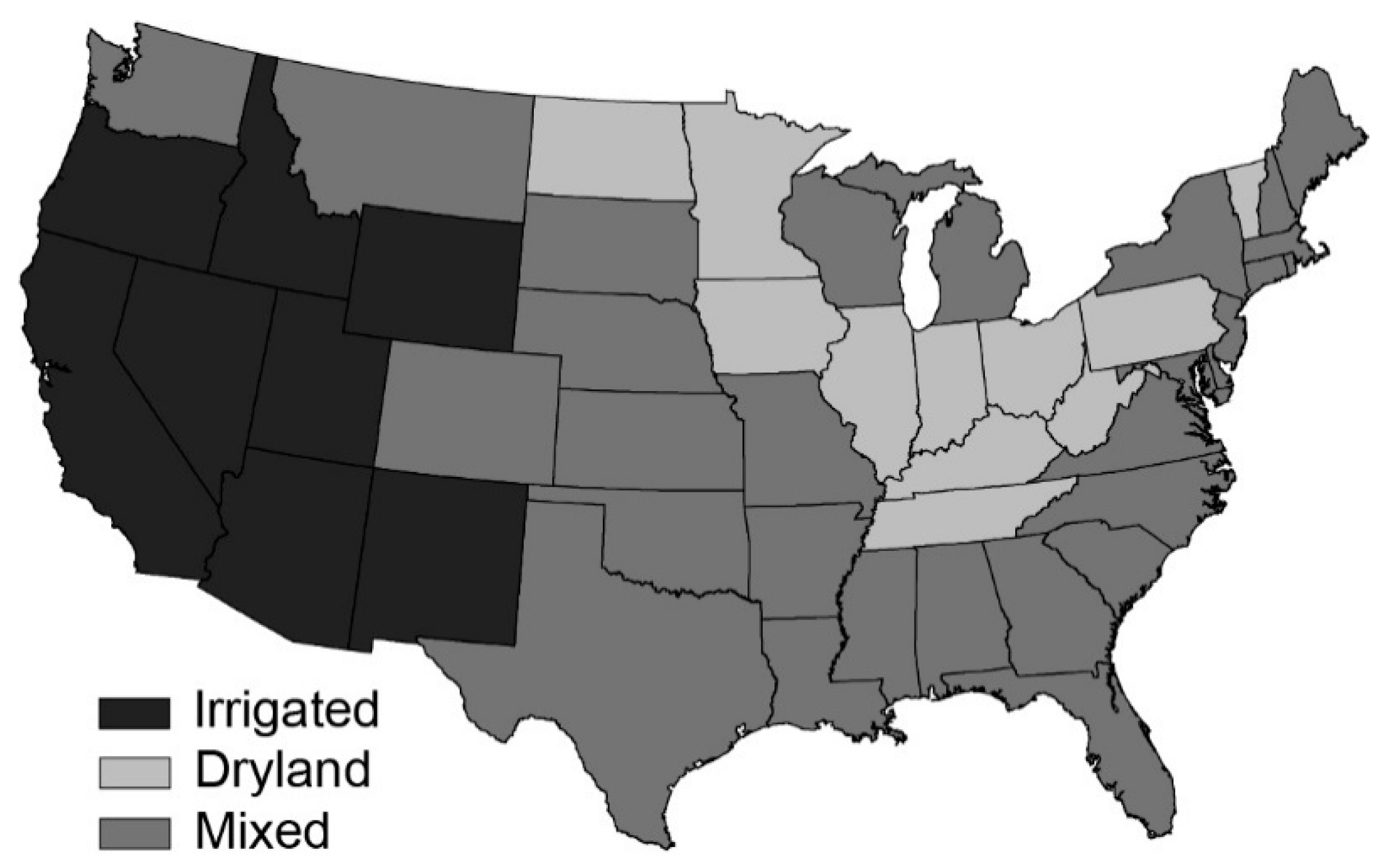
We started by grouping CONUS states into one of three categories: (1) dryland, (2) irrigated, or (3) mixed. States were assigned as “dryland” or “irrigated” using a threshold of less than 200 L per day of irrigation pumping per cropland hectare or more than 20,000 L/day/ha, respectively [7]. If irrigation fell between 200 and 20,000 L/day/ha, the state was categorized as “mixed” or marginally-dependent, with both dryland and irrigated practices. These thresholds were selected to reflect both United States Geological Survey irrigation estimates (i.e., to coordinate states with notable withdrawals) and to capture the agricultural landscape in terms of total withdrawals versus crop production (i.e., to normalize water withdrawals by total cropping area). It is important to note that irrigated states are predominantly irrigated and not entirely irrigated. The same holds true for dryland states; mixed practices can be observed to a small degree in both end-member groups. According to this classification, there are 11 dryland, 8 irrigated, and 29 mixed states, satisfying natural divisions based on common climate conditions required for the major row crops. One exception was Florida, which classifies as “irrigated” but was switched to “mixed,” since most of its irrigation is used for commodities and specialty crops outside of the five major commodity crops analyzed in this study. The summary of state classifications is shown in Figure 1.
Available yield and area data for each commodity were downloaded at the state level from the National Agricultural Statistics Survey [13]. A few states have recorded irrigated and dryland yields and areas, although these data are isolated to states above major groundwater aquifers (primarily the High Plains Aquifer states). Available irrigated and dryland yield and area data were also downloaded and included in the model construction for each end-member. Water use data used to define irrigated, mixed, and dryland states were downloaded from the United States Geological Survey for 2010, the most recent year with such data [7]. All data were processed and modeled using MATLAB R2018a (MathWorks, Natick, MA, USA).
2.2. Irrigation Yield Growth Enhancement
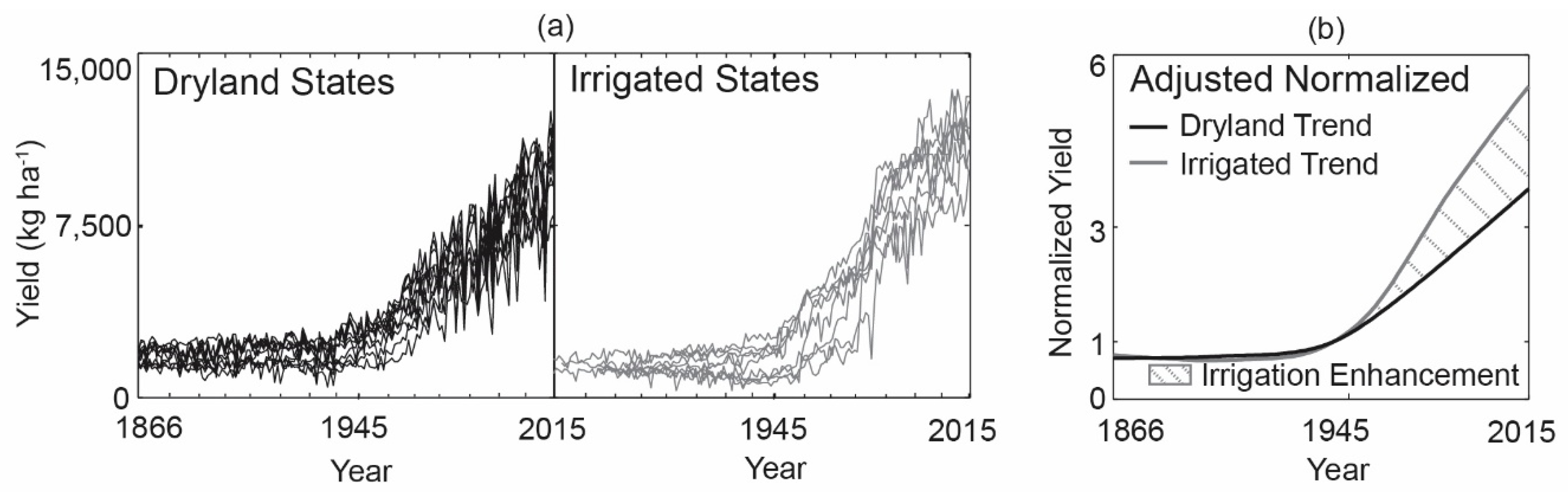
The 1940s signaled the start of a new era in agriculture, as annual yield values sharply increased relative to the consistent yields observed over the prior 80 years. This rapid increase in crop yield post-1945 can be seen in every state across the CONUS, but a distinct change in the rate of yield increase is clear in states with heavy irrigation practices relative to those with traditional dryland practices.
To demonstrate this yield difference, we plotted corn yields for dryland and irrigated states from 1866–2015, followed by area weighted averages normalized to 1945 and smoothed using a locally weighted scatterplot smooth function (lowess) in MATLAB (Figure 2). Lowess uses a regression weight function to fit a smoothed surface to the annual yield points, similar to a polynomial best-fit trend line, to reduce noise within the data and better capture long-term trends. Normalized trends were then compared across irrigated and dryland states. There was a significant divergence in the rate of yield increase between irrigated and dryland states, beginning in 1950; by 2015, average yields in irrigated states had increased 48% more than dryland states.
In theory, both groups of states should have similar yield trends post-1945, as observed pre-1945, assuming all states had access to the same innovative agricultural technologies that existed. The exception to this assumption is the access to artificial water applications through high-volume irrigation (i.e., the factors beyond irrigation have been similar across populations). Dryland states are climatically prone to both flooding and drought, which can reduce yields. Irrigated states, however, which are prone to drought but less prone to flooding, can supplement seasonal water supply to reduce the yield-limiting impact of drought conditions. This leaves the widespread use of irrigation as the only unique variable between dryland and irrigated states post-1945. The result is a more stable growing environment where water as a primary yield-limiting factor is alleviated compared to dryland states. The difference between yield trends for irrigated and dryland states can then be considered irrigation enhancement (i.e., the increase in yield due to irrigation relative to production of the same commodity in dryland states). Irrigation enhancement has been facilitated by the large-scale adoption of central pivot irrigation, beginning in the 1950s and 1960s, following the mid-century introduction of the technology. Subsequently, irrigation has continued to lead to more rapid increases in yields for over 50 years. By 2015, irrigation enhancement had led to a 545% average increase in production relative to 1945 levels, whereas non-irrigated states had seen a much smaller 366% average increase (Figure 2).
2.3. Estimating Annual Irrigated and Dryland Production
We developed a mixed end-member linear model to estimate dryland and irrigated yields for each state, and applied this model to provide more detailed yield and area statistics across mixed states dependent on both dryland and irrigated practices. A series of predictor variables were assigned to each end-member group to correlate irrigated and dryland yields relative to state-specific characteristics. Predictor variables included time (a proxy for improvements in technology, management, and crop genetics), growing season precipitation and temperature (March–October [22]), state-centered latitude and longitude, average annual recharge (calculated in ArcGIS as the statewide average recharge below agricultural lands [23,24]), and the state-average yields observed across the other major row crops [13]. A multiple linear regression model was then run between the predictor variables and the end-member yields to derive coefficients to be used to estimate dryland and irrigated yields for each mixed state, based on its predictor variables.
The variables used in the linear model to derive prediction coefficients to estimate irrigated and dryland yields for mixed states were a combination of the variables that met three criteria: (1) collectively returned the strongest correlation, (2) were individually significant at a 95% confidence interval, and (3) were statistically significant as a group at a 95% confidence interval. We also required predictor variables to return a complete list of estimated values. For example, every state has data on hay, but less than half have cotton data available. As a result, hay could be used as predictor variable for cotton, but the reverse could not be done. When irrigated and dryland yields from the Agricultural Survey were known for mixed states, they were included as part of the corresponding end-member groups.
In summary, our model estimated four main values at the state level: (1) irrigated yield, (2) dryland yield, (3) irrigated area, and (4) dryland area. Since total agricultural production can be calculated by multiplying yield and area, we were also able to estimate (5) irrigated production and (6) dryland production for each state.
Observed yield trends for each state and commodity were smoothed using the locally weighted scatterplot smooth function (lowess), as described above. We assumed that no high-volume irrigation enhancement was present before 1945, so both estimated irrigated and dryland values were adjusted to the observed 1945 value as a starting point. If observed yield trends fell below the estimated lower limit (estimated dryland) after 1945, the yield trend was assigned the lower limit value. If observed yield trends rose above the estimated upper limit (estimated irrigated), the yield trend was assigned the upper limit value. The yield trends for each state and commodity were then multiplied by the total area within the state for the corresponding commodity to quantify total production. The estimated upper and lower yield limits were also multiplied by the corresponding areas to quantify the upper and lower limits of production.
Estimated dryland yields, estimated irrigated yields, and observed production were used to quantify dryland and irrigated areas using Equation (1) through Equation (3), where is total (observed) commodity production, is dryland yield, is dryland area, is irrigated yield, is irrigated area, and is total commodity area.
Equation (1) summarizes total production across both dryland and irrigated practices, while Equation (2) is a simple summation of dryland and irrigated farmland. Equation (3) is the derived form for irrigated area using a system of equations (Equations (1) and (2)), which can also be rewritten to solve for dryland area. Our model estimates yield, and observed production is known. Thus, our area estimates are based on observed production values and estimated yields. This system of equations was applied to each mixed state to estimate dryland and irrigated areas. Calculated dryland and irrigated areas for each mixed state were then summed together to quantify the total dryland and irrigated areas for each commodity from 1950–2015.
2.4. Model Validation
Our model validation dataset consisted of yearly yield data from irrigated and dryland states. In the dryland states, yields were assumed to be completely non-irrigated, while the irrigated states had data provided for both irrigated and non-irrigated data for some commodities, and others were assumed to be solely irrigated. Calibration and validation of the linear model was conducted with two subsets of the overall dataset: (1) Yield data from odd years along with statistically significant predictor variables were used to fit model coefficients, and (2) the model was then applied to estimate yields from the remaining even years for validation. This even/odd year calibration and validation scheme was necessitated by the trending increase in yields nationwide.
2.5. Quantifying the Economic Value of Irrigation: Dominance, Dependence, and Total Revenue
Irrigation dominance for each mixed state was calculated using Equation (4):
where is irrigation dominance, is total (observed) production, is (estimated) dryland yield, is total (observed) area, is (estimated) irrigated yield, and is total average (observed) yield.
Irrigation dependence for each mixed state was calculated using Equation (5):
where is irrigation dependence. Both dominance and dependence values were then area weighted across all mixed states to estimate total values for an individual commodity using Equations (6)–(8):
where is the weight of the individual state, is total commodity area across the state, and is total commodity area across all mixed states,
where is the state weighted value, is the state value for dependence or dominance, and
where is the total commodity value for dependence or dominance.
Total dominance and dependence values for each commodity were then area weighted across all mixed states to estimate total dominance and dependence across all commodities using Equations (9)–(11):
where is the weight of the individual commodity,
where is the commodity weighted value, and
where is the total mixed state value.
The total revenue generated by irrigation was calculated using all states with significant irrigation practices (mixed + irrigated), and is described in Equation (12):
where is irrigation enhancement revenue and is 2015-adjusted market price. This process was summed across all states to get cumulative values for each commodity. Model limitations are described in Supplementary S1.
3. Results
3.1. Irrigated and Dryland Yield Model Results
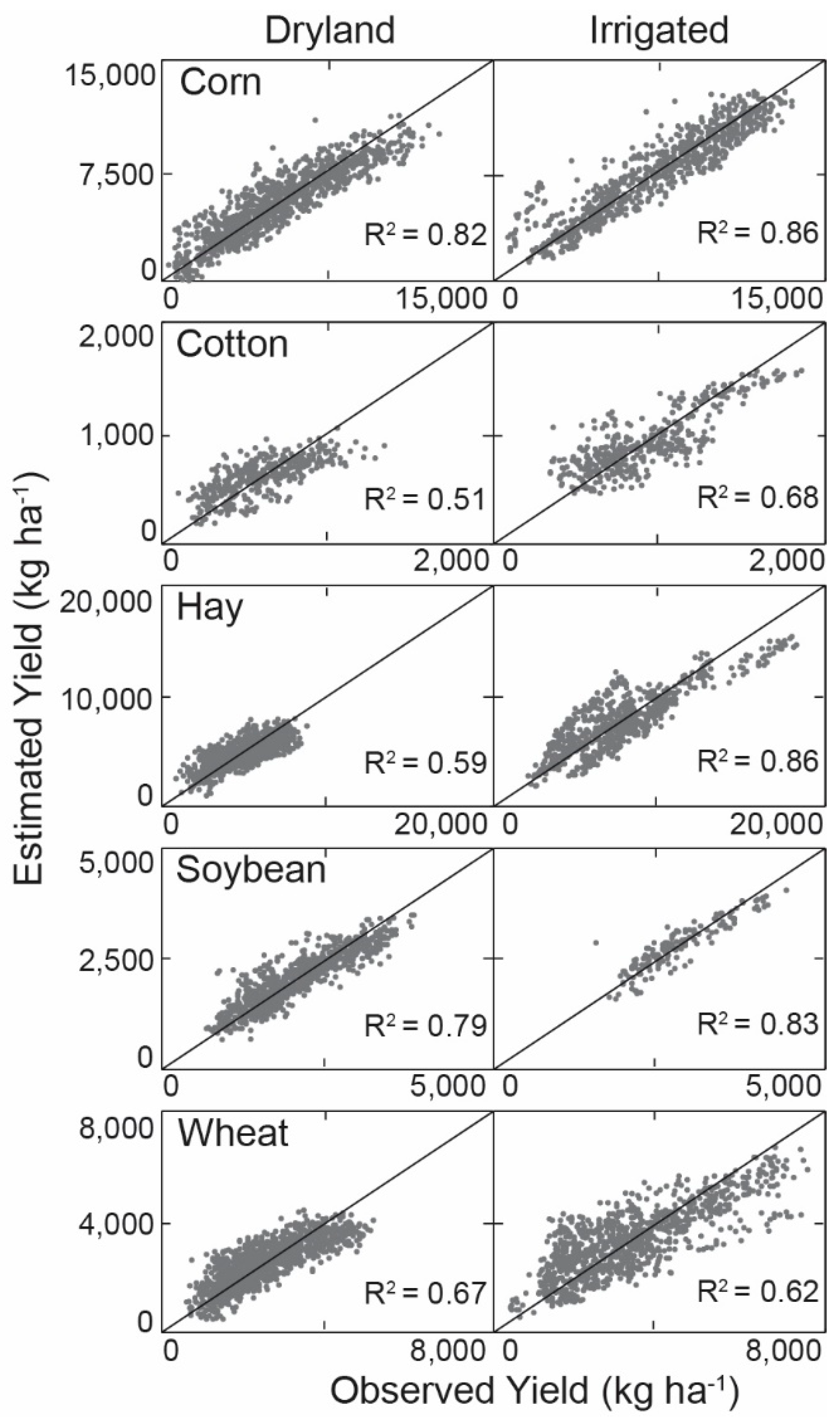
Estimated vs. observed yields for the validation years, along with coefficient of determination (R2), for each commodity across mixed states are shown in Figure 3. Supplemental validation is provided in Supplementary S2 and S3, Tables S1 and S2, and Figures S1–S3. Specifically, we observed the strongest correlations in irrigated corn, hay, and soybeans, and dryland corn. We observed the weakest correlation in dryland cotton. Collectively, irrigated estimates showed a stronger correlated fit relative to dryland conditions, as expected, due the decrease in yield variability with irrigated production. Irrigated yields also extended a larger range of values compared to dryland conditions, and higher yields collectively exhibited greater variance than lower yield values. As a whole, our coefficients of determination were strong, as crop yield is a highly variable metric.
3.2. How Have Irrigated Crop Trends Changed?
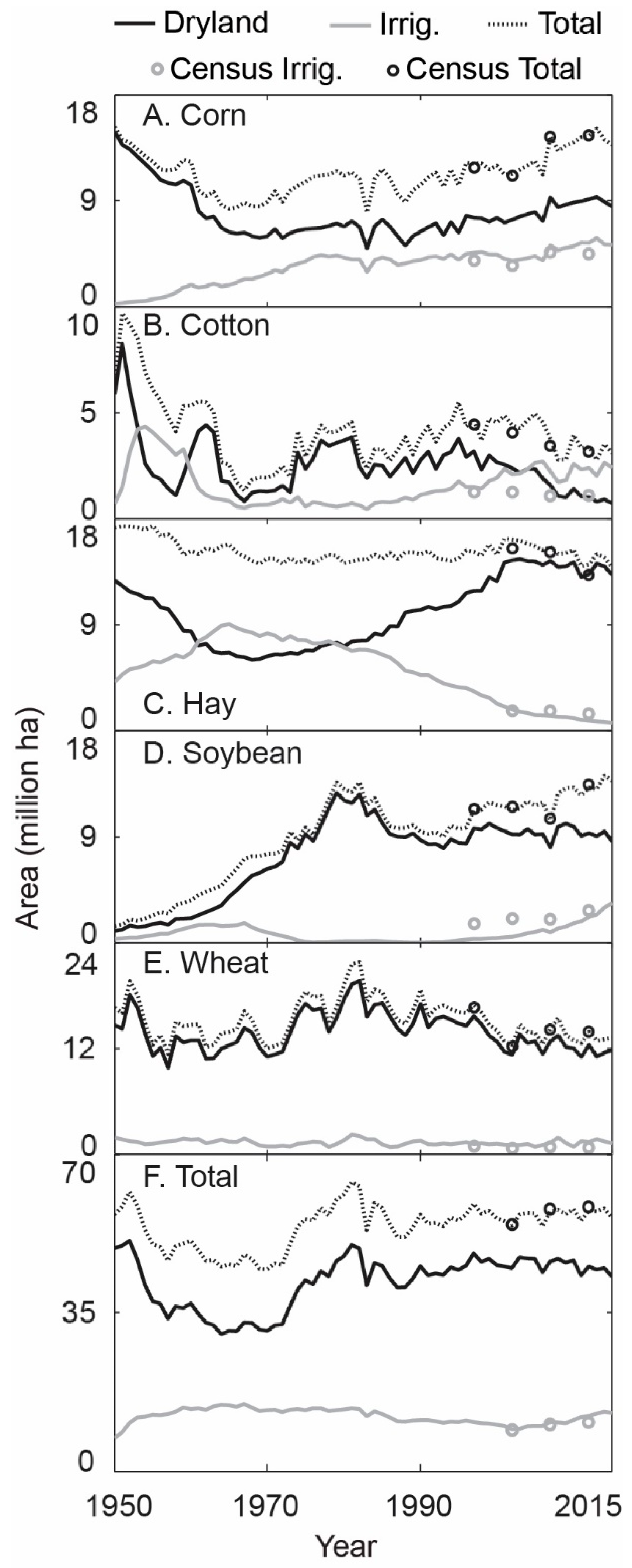
The most notable change is the increase of both irrigated and total area for corn and soybeans over the last two decades (Figure 4A,D), indicating that farmers transitioned away from other row crops to growing these irrigated commodities. Total and irrigated wheat, and hay to a lesser extent, have both declined in recent years, suggesting that these lands have been transitioned into irrigated corn and soybeans. Total irrigated area also increased, while total dryland area decreased, further demonstrating the increase in irrigation dependence (Figure 4F). From 1995–2015, total irrigated area across all mixed states increased by 2.0 million ha (18.6%); total irrigated area has increased by 2.9 million ha (28.8%) since 2005.
Since 2002, total irrigated area across mixed states steadily has increased by 39 percent, from 9.6 to 13.3 million ha in 2015, nearly matching the peaks observed from 1955–1985 (Figure 4F). Total dryland area has slowly declined since 2007, dropping from 46.3 million ha to 43.0 million ha. Interestingly, total farmland has remained stable since 1985 (~57 million ha), suggesting that any increase in total irrigated area is largely due to the conversion of pre-existing dryland area, rather than the addition of new irrigated lands. Corn, cotton, and soybeans have experienced the greatest increase in irrigated areas (Figure 4A,B,D), where hay has experienced a substantial decline in irrigated area (Figure 4C). Irrigated wheat area has remained relatively stable since 1955 (Figure 4D). The Agricultural Census data for total and irrigated areas per commodity, which were not used for model calibration, are also shown in Figure 4, and further discussion of the Census data is provided in S4.
3.3. How Dependent are Marginal States on Irrigated Production?
Here, we calculated two separate metrics to assess the degree to which marginally-irrigated states are dependent upon irrigation: (1) irrigation dominance: the degree to which the state’s average yield (or production) for a commodity is dictated by irrigated practices, and (2) irrigation dependence: the degree to which current production is dependent upon irrigation yield enhancement. Dominance is simply the fraction of irrigated area to total commodity area (assumed to be 100% for irrigated states), while dependence is impacted by: (A) irrigated per-acre yield increases relative to dryland yield, and (B) increases in irrigated area relative to total area, and is significantly less than 100% even for intensively irrigated states. Thus, any rise or fall in dependency occurs because either: (1) irrigated yields increased relative to dryland yields, or (2) irrigated area increased relative to dryland area, both of which may be influenced by technology and policy changes.
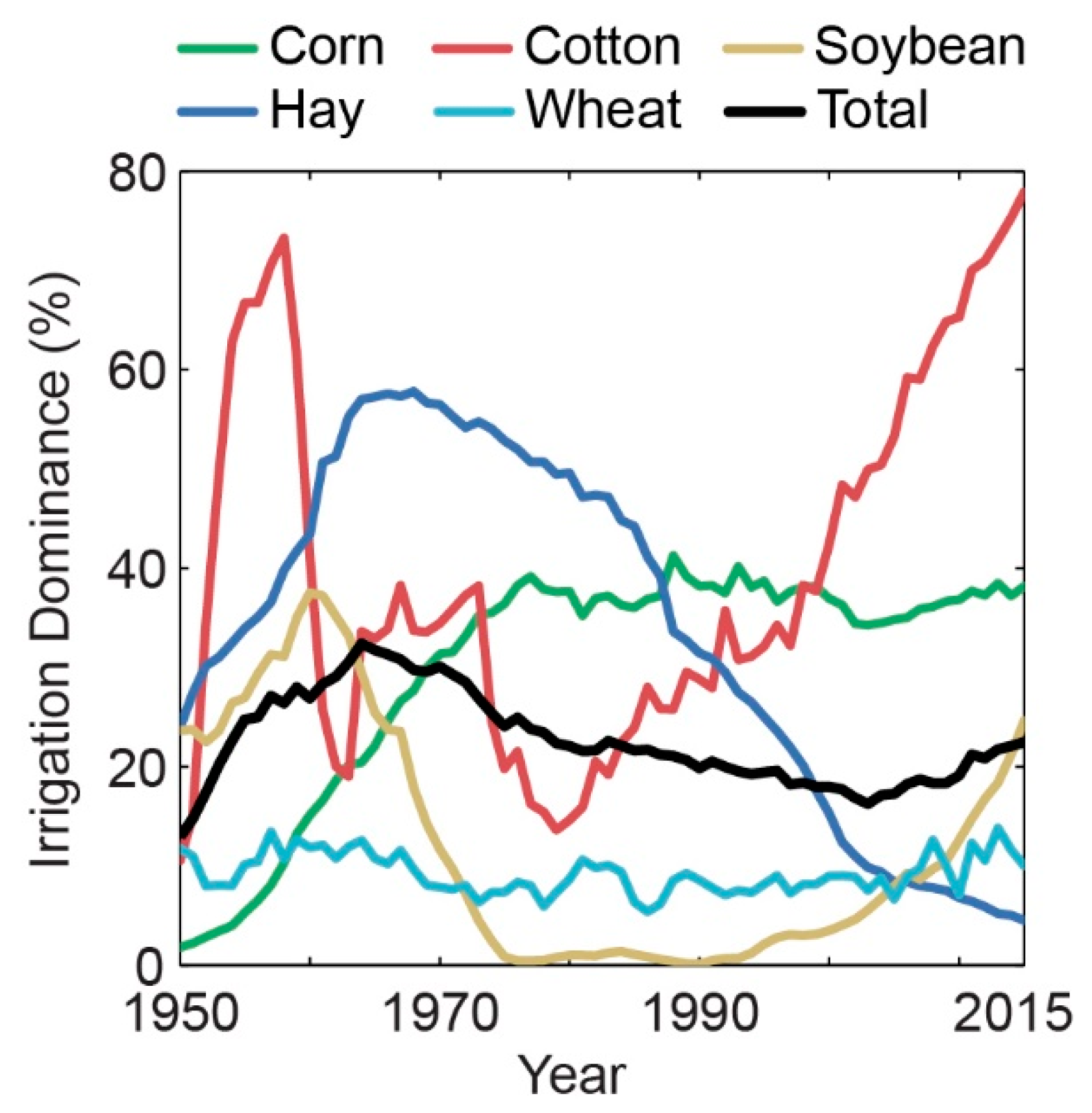
In 2015, irrigation dominance across commodities for all mixed states was 23%, indicating that about a fourth of the total production came from irrigated practices. Irrigation dominance peaked in 1964 at 32% before steadily declining to 16% in 2003. Since then, dominance has increased to its 2015 value (Figure 5). Corn production steadily increased in irrigation dominance until ~1975, after which dominance maintained a relatively steady value around the 2015 value of 38%. Irrigated dominance in cotton has been the most variable, peaking once in 1958 at 73% and again in 2015 at 78%, while rising consistently since the late 1970’s. Hay production was dominated by irrigation from ~1960–1980, with a peak of 58% in 1968; it then steadily declined to just 5% in 2015. Soybean production was originally dominated by irrigation, peaking at 38% in 1960, but quickly declined to nearly zero from 1975–1993. Since then, its irrigation dominance rapidly increased to 25% in 2015. Wheat production dominance has remained fairly stable at approximately 10% since 1950.
In 2015, irrigation dependence across all mixed states was 7%, indicating that about a tenth of all production was in excess of that which would be expected using only dryland practices on the same area. Total irrigation dependence across commodities increased rapidly from 1950 through the 1960s and has continued rising steadily, reaching peak values in 2015 (Figure 6). Corn dependence drives much of the cross-commodity total dependence, steadily increasing following a period of rapid increase through the 1970s and peaked in 2015 at 15%. Cotton dependence rapidly increased starting in 1980, and then peaked in 2011 at 14%. Hay dependence remained steady around 7% from 1964–1984, and then declined to 1% by 2015. Soybean dependence was nearly 0% from 1973 to 1993, but rapidly increased to 7% by 2015. Wheat dependence has slowly increased from 0% in 1950 to 2% in 2015.
3.4. How Much Revenue is from Irrigation Enhancement Across all States?
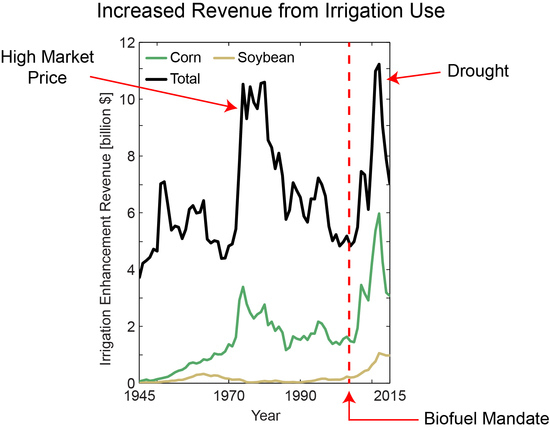
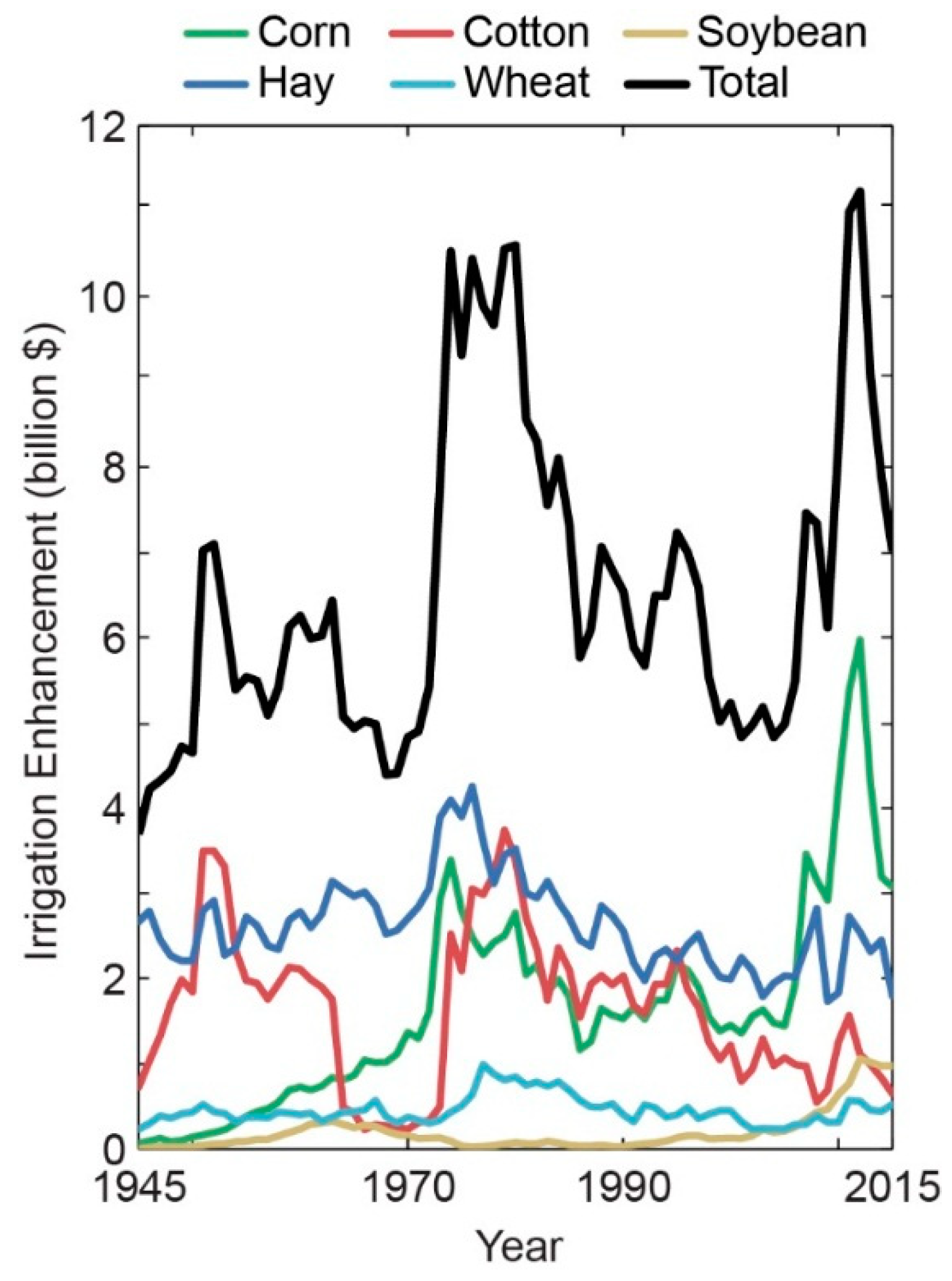
Irrigation enhancement revenue is a market-based measure of the production due to irrigation, relative to what would have been expected using production practices similar to those in dryland states (i.e., the difference between observed irrigated production by state and the average production trend derived from the normalized average of dryland states; here, revenue does not include operational costs such as system maintenance). When irrigated states are also included with mixed states (mixed + irrigated), we estimate that the total irrigation enhancement revenue since 1945 was $466 billion across the five major row crops: $187 billion for hay, $118 billion for corn, $115 billion for cotton, $32 billion for wheat, and $14 billion for soybeans (cumulative from Figure 7).
Total revenue from irrigation enhancement increased since 1945, with significant dips in 1968, 1983, and 2001–2006. In 2015, total irrigation enhancement revenue was $7.0 billion, with peaks of $11.2 billion in 2012 and $10.6 billion in 1980. Total revenue patterns after 1970 closely resembled the pattern of corn, which peaked at $6.0 billion in 2012 and is currently $3.1 billion. Prior to 1970, the total revenue pattern resembled cotton, where revenue peaked at $3.5 billion in 1951. Wheat fluctuated the least in enhancement revenue, maintaining an annual value of under $1 billion. Peak wheat revenue was $992 million in 1977, with a low of $229 million in 2002. Initially, cotton claimed the greatest boost in revenue from irrigation enhancement, peaking once at $3.5 billion in 1951, followed by a second peak of $3.7 billion in 1979, but enhanced revenue steadily declined to $648 million in 2015. Hay has largely remained the greatest source of enhancement revenue, ranging from $2 to 4 billion from 1945–2015. Much of this early revenue is attributed to the estimated inability to grow hay without irrigation in some states, resulting in all hay production becoming enhancement revenue. Soybean revenue declined from 1960–1990, with a low value of $28.3 million in 1989, but has rapidly increased in recent years, peaking at $1.1 billion in 2012. Further discussion of irrigation enhancement revenue can be found in S5.
4. Discussion
4.1. Connection to Biofuels and Drought
Three major trends have been notable since 2007: (1) increased total irrigated area (Figure 4), (2) increased percent irrigated production (Figure 5), and (3) increased irrigation enhancement revenue (Figure 7). All three trends are tightly connected to the recent increase in market demand for corn and soybeans as biofuel crops. This demand increase began in the mid-2000’s and accelerated in 2008 after the introduction of the 2008 US Farm Bill, which encouraged the production of biomass commodities and may also have encouraged improved cultivars. This connection to biofuel demand is further validated by the increase in corn and soybean area relative to other commodities, along with a concomitant increase in the total irrigated area. A change in crop choice is also apparent in the recent rise in irrigation enhancement revenue for corn and soybeans, the only two commodities with notable increases in revenue. For example, the correlation between irrigation enhancement and irrigated areas for corn and soybeans clearly increased when comparing 1985–2000 (r = 0.57 and r = 0.92, respectively) to 2000–2015 (r = 0.94 and r = 0.99, respectively), indicating an intentional selection to irrigate corn and soybeans during the current biofuel era.
It is also important to identify that the largest increase in irrigation enhancement revenue occurred in 2011–2012, which corresponds to the largest USA drought post-1945. Naturally, irrigated yields are much higher than dryland yields during a significant drought, indicating that the rapid peak in irrigation enhancement was due to climatic controls, coupled with the timing of recent increase in biofuel demand. This is an important observation, as drought intensity and frequency are projected to increase under future climate scenarios [29,30]. 2011–2012 revenue increases are most notable for corn and soybeans, though increases also occurred in cotton, wheat, and hay. One explanation for corn and soybeans experiencing the greatest spike in enhancement revenue is that a large percentage of dryland areas may also have been converted to growing corn and soybeans in regions that do not naturally accommodate these crops to capitalize on the biofuel demand [5]. Thus, the difference between irrigated and dryland yields was exacerbated when the already dry conditions for growing corn and soybeans were intensified by a significant drought. Meanwhile, areas of irrigated corn and soybean were able to maintain steady yields.
4.2. Efficiency Leads to Increased Water Use
Peak irrigation withdrawals at the national level occurred around 1980, and have since been declining [31]. Our model confirms a period of high irrigation use in 1980, but it also indicates that irrigated areas in mixed states are climbing and are not reflective of the national decline in irrigated water withdrawals. Efficient technologies coupled with purchase incentives have likely made irrigation economically feasible in these marginal states, ultimately leading to increased water use in areas outside of major aquifer regions.
The concept of increased efficiency leading to higher use and extraction is often referred to as Jevon’s paradox [32], which originated from coal and oil extraction, and has been long applied in resource economics. However, few have applied this concept to the extraction of water for irrigation [33,34,35]. Since water is often referred to as “the new oil” in popular media, it is important to validate that the efficiency–extraction relationship holds true in groundwater extraction for farming, just as in mining. Most center pivot systems have been upgraded with high-efficiency adaptations, such as low-energy precision applications (LEPA) and low-energy spray applications (LESA), helping farmers in marginal states expand irrigation practices by lowering production costs (e.g., Figure 4 [5]). Similarly, the steady increase in both irrigation enhancement revenue and irrigated area across all irrigated states, including those that are past peak groundwater extraction, further suggests that improved technologies have led to the increased groundwater withdrawals in marginal states or nearly depleted aquifer regions, in addition to other areas throughout the world [36]. Jevon’s paradox appears to hold true in irrigation just as in coal and oil, and is supported in areas where irrigation use has been expanding, which may not be economically feasible without more efficient extraction methods.
4.3. Coupled Human and Natural System
One concern for increased irrigation in mixed states is the negative environmental implications that can occur with water use intensification, in addition to declining groundwater levels. Increased groundwater extraction can cause significant land subsidence, disconnect streams and rivers, require increased energy consumption to pump water from deeper elevations, have notable impacts on regional hydrologic budgets, and cause significant regional climate effects e.g., [37,38,39,40]. However, irrigation in mixed states may never have the same environmental implications as other heavily irrigated regions, due to site-specific aquifer and climate characteristics. For example, specific yields across mixed state aquifers may not allow for the same intensity of irrigation as seen in heavily irrigated states. More humid climates in mixed regions may also be able to tolerate pumping at greater rates due to substantial recharge, as is the case in the Northern High Plains Aquifer relative to the Central and Southern High Plains Aquifer [41,42]. As a result, promoting irrigation in mixed areas that can support high levels of irrigation may be a feasible pathway to help meet future food, fiber, and biofuel demands, as water-stressed regions begin to decline in irrigated production and availability.
4.4. Implications with a Warming Climate
The Intergovernmental Panel on Climate Change estimates that across the CONUS, there will be: (1) warmer temperatures that lead to longer growing seasons, (2) higher maximum seasonal temperatures, (3) increased summer drying over mid-latitude continental interiors, and (4) more extreme El Niño patterns [29]. Conceptually, all four estimations lead to increased irrigation demand and subsequent water use through increased evaporation, increased transpiration, and drier soils. Based on the trends observed in this study, we would expect farmers to adopt new irrigation practices as an adaptation measure to combat these changing climate impacts [43]. Primarily, we would expect this new adoption to occur in predominantly dryland regions, as irrigation serves as a key mechanism for overcoming climate-related yield limiting factors, such as drought and increased temperatures (refer to Figure S2). However, irrigation is more than an adaptive measure, as it also is a feedback source to a changing climate. Increased soil moisture through irrigation substantially alters land–atmosphere interactions and impacts regional hydroclimates [39]. For example, increased irrigation in the western United States has increased precipitation in the east [44], and has been hypothesized to be a main contributor to the warming hole in the eastern United States [45]. As a result, modeling irrigation intensification may serve as a valuable component to future climate-related scenarios.
4.5. Consideration of Management Technology
Many technological management factors that were not individually analyzed here can influence crop production (e.g., use of fertilizers, weeding strategies, conventional versus no-till farming, and new cultivars). However, these technologies are not available at the scale of this study. As a result, we grouped these site-specific strategies into a proxy variable of “time,” recognizing that: (1) these factors are primarily used to maximize annual production and mitigate interannual yield variability, and (2) crop production is substantially driven by physical factors such as precipitation, temperature, and soil type. We analyzed the time proxy as an independent variable, and found it was most notable in irrigated compared to dryland conditions (Figure S2). We also analyzed the residual data for each commodity and condition using a 95% confidence interval (Figure S3), and found that few outliers exist. The implications of these two analyses suggest that: (1) the variables selected for our model captured much of the explanation for crop production (i.e., time is a robust proxy for technological management), and (2) technological advancements should be described as a means for production control that ultimately allow for consistent production increases through time by mitigating factors that lead to yield variability (e.g., drought conditions).
5. Conclusions
Comprehensive irrigated and dryland production data is critically lacking, despite the widespread use of irrigation in modern agriculture as early as the 1940’s. This study used long-term average statewide yield values to estimate irrigated and dryland production across the CONUS from 1945–2015. We then estimated the revenue earned from irrigation enhanced-yields, along with the overall dependence on irrigated production for states with mixed irrigated and dryland practices.
Based on this analysis, we have five main conclusions:
- (1)
- Irrigation enhanced revenue for the five primary commodities (corn, soy, wheat, hay, and cotton) has totaled over $465 billion since 1945, a considerable amount of revenue solely from the application of water during the growing season. Revenue has consistently increased since 1945, considerably adding to the economic risk associated with intensive irrigation practices. While many irrigated regions are not at risk for groundwater depletion, others are dangerously water stressed. Any imminent large-scale decline in irrigated area could result in a considerable economic loss. Future drought will also greatly alter the value of irrigation, as evidenced by the peak irrigation enhancement revenue during the 2012 drought, which may further increase the dependence and risk associated with artificial water applications.
- (2)
- Mixed states have become more reliant on irrigation for crop production since the turn of the 21st century, meaning the national and global market has also become reliant on irrigation for crop production. This also increases the economic risk associated with any declines in irrigated practices across the CONUS. Irrigation dominance was 23% in 2015 and rising, and irrigation dependence was 7%.
- (3)
- Total irrigated area has steadily increased across mixed states over the last two decades. Irrigated area increased 36% from just 2002–2014, with the addition of more than 1.4 million irrigated ha in this 12 year period. Total agricultural area has remained fairly constant, indicating that dryland areas are being converted to irrigated areas, rather than expanding agriculture onto new lands.
- (4)
- Crop selection in recent years has responded to the market demand for biofuel crops, trending toward irrigated biomass production. Since 2006, irrigated corn and soybean areas have increased by 34% and 207%, respectively. This has involved the addition of more than 3.6 million ha in just the past decade.
- (5)
- Reallocating irrigation applications to marginal states may be able to help reduce the water stress present in major aquifer regions. Transition of irrigation applications to marginal states could also help mitigate the economic risk associated with crop production at the national level, especially as consistent annual yields become more uncertain within major crop regions due to increased water stress (e.g., the High Plains Aquifer); this may also be possible without negatively impacting the well-being of local residents in heavily irrigated areas [46].
The data generated in this study mirror the format of the commonly used datasets reported by the United States Department of Agriculture, allowing for data processing compatibility with other efforts. The methods can also be applied at a county scale to match the interests of local management districts and statewide water resources conservation objectives [47]. In addition, the climate-related predictor variables used in the numerical model can be replaced with future climate projections at the same scale to develop estimates of feedbacks between irrigation and climate change. This study provides a robust irrigation dataset grounded in reported observations that can be used to analyze and project changes in agricultural resources.
Supplementary Materials
The following are available online at https://www.mdpi.com/2073-4441/11/7/1458/s1. Figure S1: Observed total annual production compared to estimated (dryland + irrigated) production for each commodity across all mixed states, Figure S2: Two-step regression isolating time as a predictor variable relative to all variables used in the estimation of corn production, Figure S3: Residual intervals for each commodity and condition characterized by a 95% confidence threshold, Table S1: Percent difference between 2013 estimated and observed dryland and irrigated yields for each commodity across all mixed states. Note that positive values are overestimations and negative values are underestimations, Table S2: Statistically significant (<0.05 p-value) predictor variables used to derive coefficients for estimating dryland and irrigated yields and acreages for each mixed state. Note the variable bank includes all the predictor variables tested.
Author Contributions
For research articles with several authors, a short paragraph specifying their individual contributions must be provided. The following statements should be used “Conceptualization, S.J.S. and A.D.K.; Methodology, S.J.S., A.D.K. and D.W.H.; Validation, S.J.S., A.D.K. and D.W.H.; Formal Analysis, S.J.S. and A.D.K.; Investigation, S.J.S. and A.D.K.; Data Curation, S.J.S., A.D.K. and D.W.H.; Writing–Original Draft Preparation, S.J.S., A.D.K. and D.W.H.; Writing–Review & Editing, S.J.S., A.D.K. and D.W.H.; Visualization, S.J.S., A.D.K. and D.W.H.; Supervision, A.D.K. and D.W.H.; Project Administration, D.W.H.; Funding Acquisition, A.D.K. and D.W.H.”, please turn to the CRediT taxonomy for the term explanation. Authorship must be limited to those who have contributed substantially to the work reported.
Funding
This manuscript is based upon work supported by National Science Foundation grants 1039180, and 1027253 and a USDA NIFA grants 2015-68007-23133 and 2018-67003-27406.
Acknowledgments
Any opinions, findings, and conclusions or recommendations expressed in this material are those of the authors and do not necessarily reflect the views of the National Science Foundation or the USDA National Institute of Food and Agriculture.
Conflicts of Interest
The authors declare no conflict of interest or financial disclosures to report.
References
- Schaible, G.; Aillery, M. Water conservation in irrigated agriculture: Trends and challenges in the face of emerging demands. USDA-ERS Econ. Inf. Bull. 2012. [Google Scholar] [CrossRef]
- Thompson, T.L.; Pang, H.C.; Li, Y.Y. The potential contribution of subsurface drip irrigation to water-saving agriculture in the western USA. Agric. Sci. China 2009, 8, 850–854. [Google Scholar] [CrossRef]
- Seo, S.; Segarra, E.; Mitchell, P.D.; Leatham, D.J. Irrigation technology adoption and its implication for water conservation in the Texas High Plains: A real options approach. Agric. Econ. 2008, 38, 47–55. [Google Scholar] [CrossRef]
- Li, H.; Zhao, J. Rebound Effects of New Irrigation Technologies: The Role of Water Rights. Am. J. Agric. Econ. 2018, 100, 786–808. [Google Scholar] [CrossRef]
- Smidt, S.J.; Haacker, E.M.; Kendall, A.D.; Deines, J.M.; Pei, L.; Cotterman, K.A.; Li, H.; Liu, X.; Basso, B.; Hyndman, D.W. Complex water management in modern agriculture: Trends in the water-energy-food nexus over the High Plains Aquifer. Sci. Total Environ. 2016, 566, 988–1001. [Google Scholar] [CrossRef] [PubMed]
- Pfeiffer, L.; Lin, C.C. Does efficient irrigation technology lead to reduced groundwater extraction? Empirical evidence. J. Environ. Econ. Manag. 2014, 67, 189–208. [Google Scholar] [CrossRef] [Green Version]
- USGS. USGS Water Data for the Nation; U.S. Geological Survey, National Water Information System: Washington, DC, USA, 2016. Available online: http://waterdata.usgs.gov/nwis/ (accessed on 1 May 2019).
- Deines, J.M.; Kendall, A.D.; Hyndman, D.W. Annual irrigation dynamics in the US Northern High Plains derived from Landsat satellite data. Geophys. Res. Lett. 2017, 41, 9350–9360. [Google Scholar] [CrossRef]
- Leng, G. Recent changes in county-level corn yield variability in the United States from observations and crop models. Sci. Total Environ. 2017, 607, 683–690. [Google Scholar] [CrossRef]
- Zhang, T.; Lin, X.; Sassenrath, G.F. Current irrigation practices in the central United States reduce drought and extreme heat impacts for maize and soybean, but not for wheat. Sci. Total Environ. 2015, 508, 331–342. [Google Scholar] [CrossRef] [PubMed]
- Baker, J.M.; Griffis, T.J.; Ochsner, T.E. Coupling landscape water storage and supplemental irrigation to increase productivity and improve environmental stewardship in the US Midwest. Water Resour. Res. 2012, 48, W05301. [Google Scholar] [CrossRef]
- Wilhelmi, O.V.; Wilhite, D.A. Assessing vulnerability to agricultural drought: A Nebraska case study. Nat. Hazards 2002, 25, 37–58. [Google Scholar] [CrossRef]
- NASS-USDA. Census of Agriculture; US Department of Agriculture, National Agricultural Statistics Service: Washington, DC, USA, 2019. Available online: https://quickstats.nass.usda.gov/ (accessed on 1 May 2019).
- Chen, B.; Han, M.Y.; Peng, K.; Zhou, S.L.; Shao, L.; Wu, X.F.; Wei, W.D.; Liu, S.Y.; Li, Z.; Li, J.S.; et al. Global land-water nexus: Agricultural land and freshwater use embodied in worldwide supply chains. Sci. Total Environ. 2018, 613, 931–943. [Google Scholar] [CrossRef] [PubMed]
- Takatsuka, Y.; Niekus, M.R.; Harrington, J.; Feng, S.; Watkins, D.; Mirchi, A.; Nguyen, H.; Sukop, M.C. Value of irrigation water usage in South Florida agriculture. Sci. Total Environ. 2018, 626, 486–496. [Google Scholar] [CrossRef] [PubMed]
- Boyer, C.N.; Larson, J.A.; Roberts, R.K.; McClure, A.T.; Tyler, D.D. The impact of field size and energy cost on the profitability of supplemental corn irrigation. Agric. Syst. 2014, 127, 61–69. [Google Scholar] [CrossRef]
- Brown, J.F.; Pervez, M.S. Merging remote sensing data and national agricultural statistics to model change in irrigated agriculture. Agric. Syst. 2014, 127, 28–40. [Google Scholar] [CrossRef] [Green Version]
- Neumann, K.; Stehfest, E.; Verburg, P.H.; Siebert, S.; Müller, C.; Veldkamp, T. Exploring global irrigation patterns: A multilevel modelling approach. Agric. Syst. 2011, 104, 703–713. [Google Scholar] [CrossRef]
- Shapero, M.; Dronova, I.; Macaulay, L. Implications of changing spatial dynamics of irrigated pasture, California’s third largest agricultural water use. Sci. Total Environ. 2017, 605, 445–453. [Google Scholar] [CrossRef]
- Salmerόn, M.; Purcell, L.C.; Vories, E.D.; Shannon, G. Simulation of genotype-by-environment interactions on irrigated soybean yields in the US Midsouth. Agric. Syst. 2017, 150, 120–129. [Google Scholar] [CrossRef]
- Zhang, T.; Lin, X. Assessing future drought impacts on yields based on historical irrigation reaction to drought for four major crops in Kansas. Sci. Total Environ. 2016, 550, 851–860. [Google Scholar] [CrossRef] [Green Version]
- NOAA-CDO. Climate Data Online; US Department of Commerce, The National Oceanic and Atmospheric Administration: Washington, DC, USA, 2019. Available online: https://www.ncdc.noaa.gov/cdo-web/ (accessed on 1 May 2019).
- Homer, C.; Dewitz, J.; Yang, L.; Jin, S.; Danielson, P.; Xian, G.; Coulston, J.; Herold, N.; Wickham, J.; Megown, K. Completion of the 2011 National Land Cover Database for the conterminous United States-Representing a decade of land cover change information. Photogramm. Eng. Remote Sens. 2015, 81, 345–354. [Google Scholar]
- USGS. Estimated Mean Annual Natural Ground-Water Recharge in the Conterminous United States; U.S. Geological Survey, National Water Information System: Washington, DC, USA, 2013. Available online: https://water.usgs.gov/GIS/metadata/usgswrd/XML/rech48grd.xml (accessed on 1 May 2019).
- NASS-USDA. Census of Agriculture; US Department of Agriculture, National Agricultural Statistics Service: Washington, DC, USA, 1997.
- NASS-USDA. Census of Agriculture; US Department of Agriculture, National Agricultural Statistics Service: Washington, DC, USA, 2002.
- NASS-USDA. Census of Agriculture; US Department of Agriculture, National Agricultural Statistics Service: Washington, DC, USA, 2007. Available online: https://www.agcensus.usda.gov/Publications/2007/Full_Report/Volume_1,_Chapter_1_US/usv1.pdf (accessed on 1 May 2019).
- NASS-USDA. Census of Agriculture; US Department of Agriculture, National Agricultural Statistics Service: Washington, DC, USA, 2012. Available online: https://www.agcensus.usda.gov/Publications/2012/Full_Report/Volume_1,_Chapter_1_US/usv1.pdf (accessed on 1 May 2019).
- IPCC, Intergovernmental Panel on Climate Change. Climate Change 2014–Impacts, Adaptation and Vulnerability: Regional Aspects; Cambridge University Press: Cambridge, UK, 2014. [Google Scholar]
- Karl, T.R.; Trenberth, K.E. Modern global climate change. Science 2003, 302, 1719–1723. [Google Scholar] [CrossRef] [PubMed]
- Maupin, M.A.; Kenny, J.F.; Hutson, S.S.; Lovelace, J.K.; Barber, N.L.; Linsey, K.S. Estimated use of water in the United States in 2010 (No. 1405). US Geol. Surv. 2014. [Google Scholar] [CrossRef]
- Jevons, W.S. The Coal Question: An Inquiry Concerning the Progress of The Nation, and the Probable Exhaustion of the Coal-Mines; Macmillan: London, UK, 1865. [Google Scholar]
- Berbel, J.; Mateos, L. Does investment in irrigation technology necessarily generate rebound effects? A simulation analysis based on an agro-economic model. Agric. Syst. 2014, 128, 25–34. [Google Scholar] [CrossRef]
- Dumont, A.; Mayor, B.; López-Gunn, E. Is the rebound effect or Jevons paradox a useful concept for better management of water resources? Insights from the Irrigation Modernisation Process in Spain. Aquat. Procedia 2013, 1, 64–76. [Google Scholar] [CrossRef]
- Gomez, C.M.; Gutierrez, C. Enhancing irrigation efficiency but increasing water use: The Jevons’ paradox. In Proceedings of the EAAE Congress: Change and Uncertainty Challenges for Agriculture, Food and Natural Resources, Zurich, Switzerland, 30 August–2 September 2011. [Google Scholar]
- Perry, C.; Steduto, P.; Karajeh, F. Does Improved Irrigation Technology Save Water? A Review of the Evidence; Food and Agriculture Organization of the United Nations: Cairo, Egypt, 2017; p. 42. [Google Scholar]
- De Angelis, A.; Dominguez, F.; Fan, Y.; Robock, A.; Kustu, M.D.; Robinson, D. Evidence of enhanced precipitation due to irrigation over the Great Plains of the United States. J. Geophys. Res.-Atmos. 2010, 115, D15115. [Google Scholar] [CrossRef]
- Kustu, M.D.; Fan, Y.; Rodell, M. Possible link between irrigation in the US High Plains and increased summer streamflow in the Midwest. Water Resour. Res. 2011, 47, W03522. [Google Scholar] [CrossRef]
- Pei, L.; Moore, N.; Zhong, S.; Kendall, A.D.; Gao, Z.; Hyndman, D.W. Effects of irrigation on summer precipitation over the United States. J. Clim. 2016, 29, 3541–3558. [Google Scholar] [CrossRef]
- Scanlon, B.R.; Faunt, C.C.; Longuevergne, L.; Reedy, R.C.; Alley, W.M.; McGuire, V.L.; McMahon, P.B. Groundwater depletion and sustainability of irrigation in the US High Plains and Central Valley. Proc. Natl. Acad. Sci. USA 2012, 109, 9320–9325. [Google Scholar] [CrossRef] [Green Version]
- Breña-Naranjo, J.A.; Kendall, A.D.; Hyndman, D.W. Improved methods for satellite-based groundwater storage estimates: A decade of monitoring the high plains aquifer from space and ground observations. Geophys. Res. Lett. 2014, 41, 6167–6173. [Google Scholar] [CrossRef]
- Haacker, E.M.K.; Kendall, A.D.; Hyndman, D.W. Water Level Declines in the High Plains Aquifer: Predevelopment to Resource Senescence. Groundwater 2015, 54, 231–242. [Google Scholar] [CrossRef]
- Haacker, E.M.; Cotterman, K.A.; Smidt, S.J.; Kendall, A.D.; Hyndman, D.W. Effects of management areas, drought, and commodity prices on groundwater decline patterns across the High Plains Aquifer. Agric. Water Manag. 2019, 218, 259–273. [Google Scholar] [CrossRef]
- Alter, R.E.; Fan, Y.; Lintner, B.R.; Weaver, C.P. Observational evidence that Great Plains irrigation has enhanced summer precipitation intensity and totals in the Midwestern United States. J. Hydrometeorol. 2015, 16, 1717–1735. [Google Scholar] [CrossRef]
- Partridge, T.F.; Winter, J.M.; Osterberg, E.C.; Hyndman, D.W.; Kendall, A.D.; Magilligan, F.J. Spatially distinct seasonal patterns and forcings of the U.S. warming hole. Geophys. Res. Lett. 2018, 45, 2055–2063. [Google Scholar] [CrossRef]
- Lauer, S.; Sanderson, M. Irrigated agriculture and human development: A county-level analysis 1980–2010. Environ. Dev. Sustain. 2019, 1–17. [Google Scholar] [CrossRef]
- Dolan, F.C.; Cath, T.Y.; Hogue, T.S. Assessing the feasibility of using produced water for irrigation in Colorado. Sci. Total Environ. 2018, 640, 619–628. [Google Scholar] [CrossRef] [PubMed]
Figure 1.
State classifications of dryland, irrigated, or mixed defined by cropland area per irrigated water use threshold values.
Figure 1.
State classifications of dryland, irrigated, or mixed defined by cropland area per irrigated water use threshold values.

Figure 2.
Corn yields for dryland and irrigated states (a) and yield enhancement due to irrigation (b) demonstrated using 1945-normalized locally weighted means [13].
Figure 2.
Corn yields for dryland and irrigated states (a) and yield enhancement due to irrigation (b) demonstrated using 1945-normalized locally weighted means [13].

Figure 3.
Multiple linear regression model showing observed versus estimated yields for the validation years across all irrigated and dryland states. Note that axes have different scales.
Figure 3.
Multiple linear regression model showing observed versus estimated yields for the validation years across all irrigated and dryland states. Note that axes have different scales.

Figure 4.
Estimated dryland, irrigated, and total areas for each commodity across all mixed states. Included are the areas reported in the National Agricultural Statistics Service Census history [25,26,27,28]. Panel (A) displays the dryland, irrigated, and total area trends for corn, Panel (B) for cotton, Panel (C) for hay, Panel (D) for soybeans, and Panel (E) for wheat. Panel (F) is the summation of the previous panels to highlight total area trends.

Figure 5.
Irrigation dominance for each commodity across all mixed states.

Figure 6.
Irrigation dependence for each commodity across all mixed states.

Figure 7.
Annual irrigation enhancement revenue for each commodity across all states with irrigation.
Figure 7.
Annual irrigation enhancement revenue for each commodity across all states with irrigation.

© 2019 by the authors. Licensee MDPI, Basel, Switzerland. This article is an open access article distributed under the terms and conditions of the Creative Commons Attribution (CC BY) license (http://creativecommons.org/licenses/by/4.0/).
Share and Cite
MDPI and ACS Style
Smidt, S.J.; Kendall, A.D.; Hyndman, D.W. Increased Dependence on Irrigated Crop Production Across the CONUS (1945–2015). Water 2019, 11, 1458. https://doi.org/10.3390/w11071458
AMA Style
Smidt SJ, Kendall AD, Hyndman DW. Increased Dependence on Irrigated Crop Production Across the CONUS (1945–2015). Water. 2019; 11(7):1458. https://doi.org/10.3390/w11071458
Chicago/Turabian StyleSmidt, Samuel J., Anthony D. Kendall, and David W. Hyndman. 2019. "Increased Dependence on Irrigated Crop Production Across the CONUS (1945–2015)" Water 11, no. 7: 1458. https://doi.org/10.3390/w11071458
Note that from the first issue of 2016, this journal uses article numbers instead of page numbers. See further details here.