Secondary Flow Effects on Deposition of Cohesive Sediment in a Meandering Reach of Yangtze River


1
State Key Laboratory of Hydroscience and Engineering, Tsinghua University, Beijing 100084, China
2
National Inland Waterway Regulation Engineering Research Center, Chongqing Jiaotong University, Chongqing 400074, China
*
Author to whom correspondence should be addressed.
Water 2019, 11(7), 1444; https://doi.org/10.3390/w11071444
Submission received: 27 May 2019
/
Revised: 28 June 2019
/
Accepted: 9 July 2019
/
Published: 12 July 2019
(This article belongs to the Special Issue The Application of Hydraulic and Sediment Transport Models in Fluvial Geomorphology)
Abstract
:Few researches focus on secondary flow effects on bed deformation caused by cohesive sediment deposition in meandering channels of field mega scale. A 2D depth-averaged model is improved by incorporating three submodels to consider different effects of secondary flow and a module for cohesive sediment transport. These models are applied to a meandering reach of Yangtze River to investigate secondary flow effects on cohesive sediment deposition, and a preferable submodel is selected based on the flow simulation results. Sediment simulation results indicate that the improved model predictions are in better agreement with the measurements in planar distribution of deposition, as the increased sediment deposits caused by secondary current on the convex bank have been well predicted. Secondary flow effects on the predicted amount of deposition become more obvious during the period when the sediment load is low and velocity redistribution induced by the bed topography is evident. Such effects vary with the settling velocity and critical shear stress for deposition of cohesive sediment. The bed topography effects can be reflected by the secondary flow submodels and play an important role in velocity and sediment deposition predictions.
1. Introduction
Helical flow or secondary flow caused by centrifuge force in meandering rivers plays an important role in flow and sediment transport. It redistributes the main flow and sediment transport, mixes dissolved and suspended matter, causes additional friction losses, and additional bed shear stress, which are responsible for the transverse bed load sediment transport [1,2,3]. Moreover, the secondary flow may affect lateral evolution of river channels [4,5,6]. Extensive researches have been conducted about secondary flow effects on flow and sediment transport, especially bed load in a singular bend [7] or meandering channels of laboratory scale [8] and rivers of field scale [9,10]. However, few researches focus on suspended load transport. In China, sediment transport in most rivers is dominated by suspended load, such as Yangtze River and Yellow River. On the Yangtze River, the medium diameter of sediment from upstream is ~0.01 mm [11], which has taken on cohesive properties to some extent [11,12]. More importantly, these cohesive suspended sediments have been extensively deposited in several reaches which have blocked the waterway in Yangtze River [13]. As most of these reaches are meanders with a central bar located in the channel, to what extent the secondary flow has affected the cohesive suspended sediment deposition should be investigated.
Cohesive sediment deposition is controlled by bed shear stress [14], which is determined by the flow field. In order to investigate the secondary flow effects on cohesive sediment transport, its effects on flow field should be considered first. Secondary flow redistributes velocities, which means the high velocity core shifts from the inner bank to the outer bank of the bend [15,16]. Saturation of secondary flow takes place in sharp bends [17]. Due to the inertia, the development of secondary flow lags behind the curvature called the phase lag effect [18]. All these findings mainly rely on laboratory experiments or small rivers with a width to depth radio less than 30 [19] probably resulting in an exaggeration of secondary flow. When it comes to natural meandering or anabranching rivers, especially large or mega rivers, secondary flow may be absent or limited in a localized portion of the channel width [20,21,22,23,24]. However, those researches are only based on field surveys and mainly focused on influences of bifurcation or confluence of mega rivers with low curvatures and significant bed roughness [23] at the scale of individual hydrological events. On contrary, Nicholas [25] emphasized the role of secondary flow played in generating high sinuosity meanders via simulating a large meandering channel evolution on centennial scale. Maybe it depends on planimetric configurations, such as channel curvature, corresponding flow deflection [26] and temporal scales. Therefore, whether secondary flow exists and has the same effects on the flow field in a meandering mega river as that in laboratory experiments should be further investigated. Besides, the long-term hydrograph should be taken into account.
As to its effects on bed morphology, secondary flow induced by channel curvature produces a point bar and pool morphology by causing transversal transport of sediment, which in turn drives lateral flow (induced by topography) known as topographic steering [9] which plays an even more significant role in meandering dynamics than that curvature-induced secondary flow [3]. The direction of sediment transport is derived from that of depth-averaged velocity due to the secondary flow effect, which has been accounted for in 2D depth-averaged models and proved to contribute to the formation of local topography [4,5,6,27], especially bar dynamics [28,29], and even to channel lateral evolution [4,6,30]. Although Kasvi et al. [31] has pointed that the exclusion of secondary flow has a minor impact on the point bar dynamics, temporal scale effects remain to be investigated as the authors argued for only one flood event has been considered in their research and the inundation time may affect the effects of secondary flow [32]. Those researches have enriched our understandings of mutual interactions of secondary flow and bed morphology. However, they mainly focused on bed load sediment transport, whereas the world largest rivers are mostly fine-grained system [21] and are dominated by silt and clay, such as Yangtze River [11,12]. Fine-grained suspended material ratio controls the bar dynamics and morphodynamics in mega rivers [23,33]. As is known, such fine-grained sediment is common in estuarine and coastal areas. However, how they work under the impacts of secondary flow in mega rivers is still up in the air and the temporal effects of secondary flow should be investigated.
Numerical method provides a convenient tool for understanding river evolution in terms of hydrodynamics and morphodynamics in addition to the laboratory experiments and field surveys. The 2D depth-averaged model is preferable because it keeps as much detailed information as possible on the one hand and remains practical for investigation of long-term and large-scale fluvial processes on the other hand. The main shortcoming of the 2D depth-averaged model is that the vertical structure of flow has been lost due to the depth-integration of the flow momentum and suspended sediment transport equations, and thus the secondary flow effects on the flow field and suspended sediment transport are neglected. These effects can be retrieved by incorporating closure correction submodels into the 2D depth-averaged model. In order to account for these effects on the flow field, various correction submodels have been proposed by many researchers [34,35,36,37,38]. The differences among these models are whether or not they consider (1) the feedback effects between main flow and secondary flow and (2) the phase lag effect of the secondary flow caused by inertia. Models neglecting the former one are classified as linear models, in contrast to nonlinear models which consider such effects [1,38]. The nonlinear models [1,39] based on the linear ones are more suitable for flow simulation of sharp bends [1,2]. The phase lag effect, which is obviously pronounced in meandering channels [40], has been thought to be important in sharp bends especially with pronounced curvature variations [2], and proven to influence bar dynamics considerably [29]. Although the performances of those above mentioned models have been extensively tested by laboratory scale bends, their applicability to field meandering rivers, especially mega rivers, needs to be further investigated. Besides, which model is preferable in flow simulation of meandering channels of field mega scale remains to be answered.
To consider the secondary flow effects on the suspended sediment transport, closure submodels should be coupled to the sediment module of the 2D depth-averaged models in a similar way to the flow module [41]. However, as to the cohesive sediment transport, it is mainly related to the bed shear stress determined by the flow field. Besides, according to field survey of two reaches of Yangtze River by Li et al. [11], cohesive sediment transport is controlled by the depth-averaged velocity. Therefore, only the secondary flow effects on flow field are considered to further analyze their effects on bed morphology here. In addition, the turbulence models should be considered in the 2D depth-averaged model, especially when there are recirculating flows [34]. Based on the previous research work [34,36], the depth-averaged parabolic eddy viscosity model can be applied.
This paper aims to investigate the secondary flow effects on cohesive sediment deposition in meandering reach of field mega scale during an annual hydrography. The following questions will be addressed; (1) whether secondary flow effects on the flow field can be reflected by typical secondary flow correction models in such mega meandering rivers as laboratory meandering channels, (2) which model should be given priority to flow simulation in meandering channels of such scale, and (3) what the temporal influence of secondary flow is on bed morphology variations associated with cohesive sediment deposition. The contents of this paper are as follows; three secondary flow submodels referring to the aforementioned different effects have been selected from the literature—Lien et al. [37], Bernard [35], and Blankaert and de Vriend [1] models—to reveal secondary flow impacts and distinguish their performances on flow simulation in meandering channels of this mega scale first, and the preferable model is selected. Then, the corresponding model is applied to investigate secondary flow effects on bed morphology variations related with cohesive sediment deposition during an annual hydrograph. Finally, the correction terms representing secondary flow effects have been analyzed to justify their functionalities and performances of these models in meandering channels of such scale. Besides, the roles of cohesive sediment played in secondary flow effects have been investigated as well. The main contributions of this paper are three-fold: (1) the L model has been found to outperform the other models in flow simulation of the field mega scale meandering reach; (2) the bed topography effects have been identified to be reflected by the secondary flow submodels, and the transverse bed topography plays a more important role than the longitudinal one and results in the great improvements of velocity and sediment deposition predictions of the L model in this reach; and (3) secondary flow effects on cohesive sediment deposition become obvious during the last period of an annual hydrography when the sediment concentration is low and the transverse bed topography has been formed. Such effects on the predicted amount of deposition vary with the cohesive sediment properties.
2. Methods
A 2D depth-averaged model (Section 2.1, referred to as the N model hereafter) has been improved by considering secondary flow effects and cohesive sediment transport. Secondary flow module (Section 2.2) incorporates three different submodels to reflect its different effects, together with the sediment module (Section 2.3) are described briefly. All the equations are solved in orthogonal curvilinear coordinates.
2.1. Flow Equations
The unsteady 2D depth-averaged flow governing equations are expressed as follows [42]
where ξ and η = longitudinal and transverse direction in orthogonal curvilinear coordinates, respectively; h1 and h2 = metric coefficients in ξ and η directions, respectively; J = h1h2; g = acceleration gravity, m/s2; = (U, V) depth-averaged resultant velocity vector and (U, V) = depth-averaged velocity in ξ and η directions, separately; H = water depth; Z = water surface elevation; C = Chezy factor; νe = eddy viscosity; and Sξ and Sη = correction terms related to the vertical nonuniform distribution of velocity.
2.2. Secondary Flow Equations
In order to consider different effects of secondary flow on flow, three secondary flow models are selected from literature to calculate the dispersion terms (Sξ, Sη) in Equations (2) and (3). Among them, the Lien et al. [37] (L) model has been widely applied, which ignores the secondary flow phase lag effect and is suitable for fully developed flows. As secondary flow lags behind the driving curvature due to inertia [2], it will take a certain distance for secondary flow to fully develop, especially in meandering channels. There are several models using a depth-averaged transport equation to consider these phase lag effect, such as the Delft-3D [43] model, Hosoda et al. [44] model, and Bernard [35] model. The Delft-3D model has two correction coefficients to calibrate and Hosoda model is complex to use. In addition, both of them focus on flow simulation in channels with a single bend. In contrast, Bernard (B) model is simple, practicable and has been validated by several meandering channels. Moreover, the sidewall boundary conditions considered by B model is more reasonable, that is, the production of secondary flow approaches zero on the sidewalls [16]. Therefore, the B model is selected as another representative model. Because the above mentioned two models are linear models which are theoretically only applicable to mildly curved bends, a simple nonlinear (NL) model [1] is selected as a typical model to reflect the saturation effect of secondary flow [17] in sharply curved bends. All of the three models can reflect the velocity redistribution phenomenon caused by secondary flow at different levels. These models serve as submodels coupled to the 2D hydrodynamic model to account for different effects of secondary flow on flow field. The major differences of them are summarized in Table 1, while L and B models can refer to the authors [45] for more details. Only NL model are briefly described as follows.
Based on linear models, the NL model is able to consider the feedback effects between secondary flow and main flow to reflect the saturation effect through a bend parameter β [1] (Equation (10)). However, the NL model proposed by Blanckaert and de Vriend [1] is limited to the centerline of the channel. Ottevanger [46] extended the model to the whole channel width through an empirical power law (fw, Equation (9)). This method is as follows
Ti,j (i, j = 1,2) is called dispersion terms [37]. When the L model is adopted as the linear model, Ti,j is expressed as
where κ = the Von Karman constant, 0.4; r = the channel centerline, m; fw = the empirical power law equation over the channel width; FF1, FF2 = the shape coefficients related to the vertical profiles of velocity which can refer to Lien et al. [37] for details; and fsn(β) and fnn(β) are the nonlinear correction coefficients expressed as Equations (7) and (8) [47], which directly reflect the saturation effect of secondary flow [17].
β = the bend parameter which is a control parameter distinguishing the linear and nonlinear models; αs = the normalized transversal gradient of the longitudinal velocity U at the centerline; and nc = the position of channel centerline.
The phase lag effect of secondary flow is considered with the following transport equations [46].
λ = the adaption length described by Johannesson and Parker [18]. Y = the terms referring to fsn, fnn in Equation (6), Ye = the fully developed value of Y.
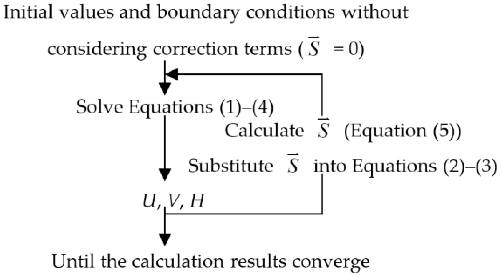
As L, B, and NL models serve as closure submodels in hydrodynamic Equations (1)–(4), the correction terms (Sξ and Sη) are associated with the computed mean flow field, and the information on the relative variables of correction terms is available when solving these submodels. This is similar to the way to solve turbulence submodels. Detailed procedure for solving the NL model is shown in Figure 1. Equations (1)–(4) are solved first without considering the correction terms (Sξ and Sη) for water depth and depth-averaged velocity. The nonlinear parameters in Equations (7)–(11) have been calculated next. Afterwards, the transport Equation (12) is solved for evaluating dispersion terms (Ti,j, Equation (6)) and (Sξ and Sη) (Equation (5)). The correction terms (Sξ and Sη) are then included in Equations (1)–(4), which are solved again to get new information on the mean flow field. The procedure continues until no significant variations in the magnitude of depth, velocity, and other variables in the model (Figure 1).
2.3. Cohesive Sediment Transport Equations
The cohesive sediment transport equation is similar to the noncohesive sediment transport equation [48], except the method to calculate the net exchange rate (Db − Eb) [14].
where C = the sediment concentration, kg·m−3; Db and Eb = the erosion and deposition rate respectively, kg·m−2·s−1, which are calculated [14] as follows
where α = deposition coefficient calculated by Equation (15); ωs = settling velocity, m·s−1.
where τb = the bed shear stress, Pa; τcd = the critical shear stress for deposition, Pa.
where n = an empirical coefficient; M = the erosion coefficient, kg·m−2·s−1; and τce = the critical shear stress for erosion, Pa.
Most of the model parameters used for cohesive sediment calculation (Table 2) have been calibrated and validated by the sedimentation process of the Three Gorges Reservoir on Yangtze River [48], where the study area of this paper is located. A larger value of settling velocity is chosen from measurements by Li et al. [11,12] because only the medium diameter of the sediment is considered in this study.
The morphological evolution due to cohesive sediment transport is calculated by the net sediment exchange rate (Db − Eb), in the same way as noncohesive suspended sediment calculation does. The flow and sediment modules are solved in an uncoupled way. Details of the numerical method can be found in Wang et al. [42]. Central difference explicit scheme is applied to Equation (5), and Equations (12) and (13) are solved by QUICK (Quadratic Upstream Interpolation for Convective Kinematics) finite difference scheme.
3. Study Case
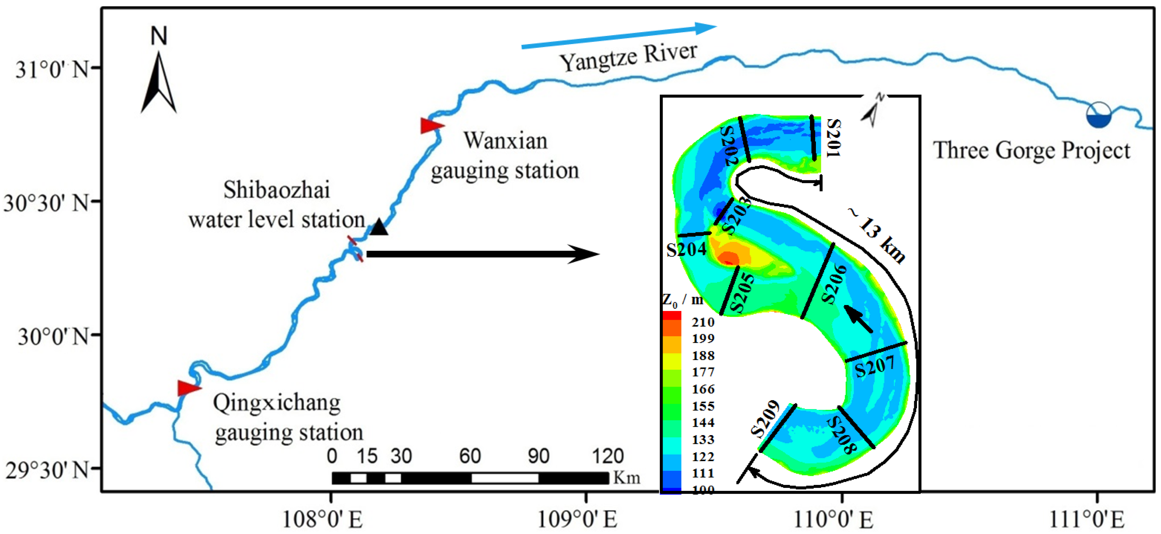
The Hunghuacheng reach (HHC, Figure 2), located 364 km upstream from the Three Gorges Project (TGP), is approximately 13 km long, consisting two sharply curved bends with a center bar named “Huanghuacheng” splitting the reach into two branches. It belongs to the back water zone of TGP. The large mean annual discharge (32,000 m3·s−1) makes it a mega river reach [49]. Measurements of bed topographies and bed material size are taken at nine cross-sections from S201 to S209 twice each year. Due to huge amount of cohesive sediment siltation, the left branch of this reach has been blocked in September 2010 [13]. Secondary flow models are applied to this reach because the secondary flow caused by the upstream bend of this reach plays an important role in channel morphodynamics [50,51]. Also, it has been shown that similar models perform well in confluence [38] and braided rivers [25], which justify the application of these models in this reach.
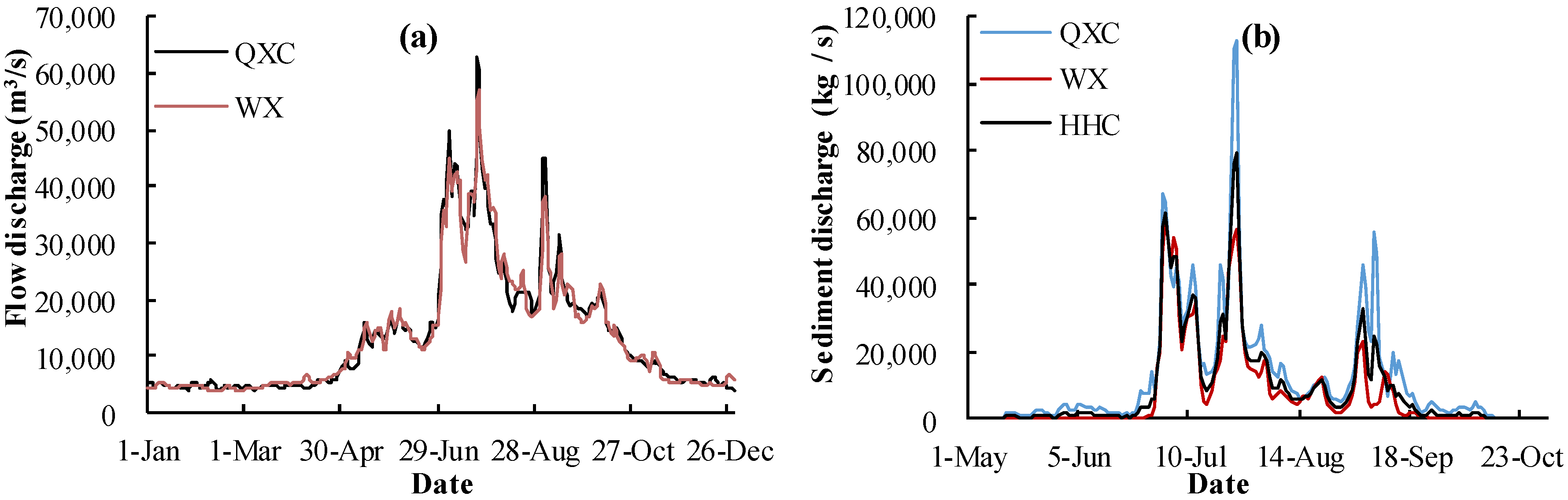
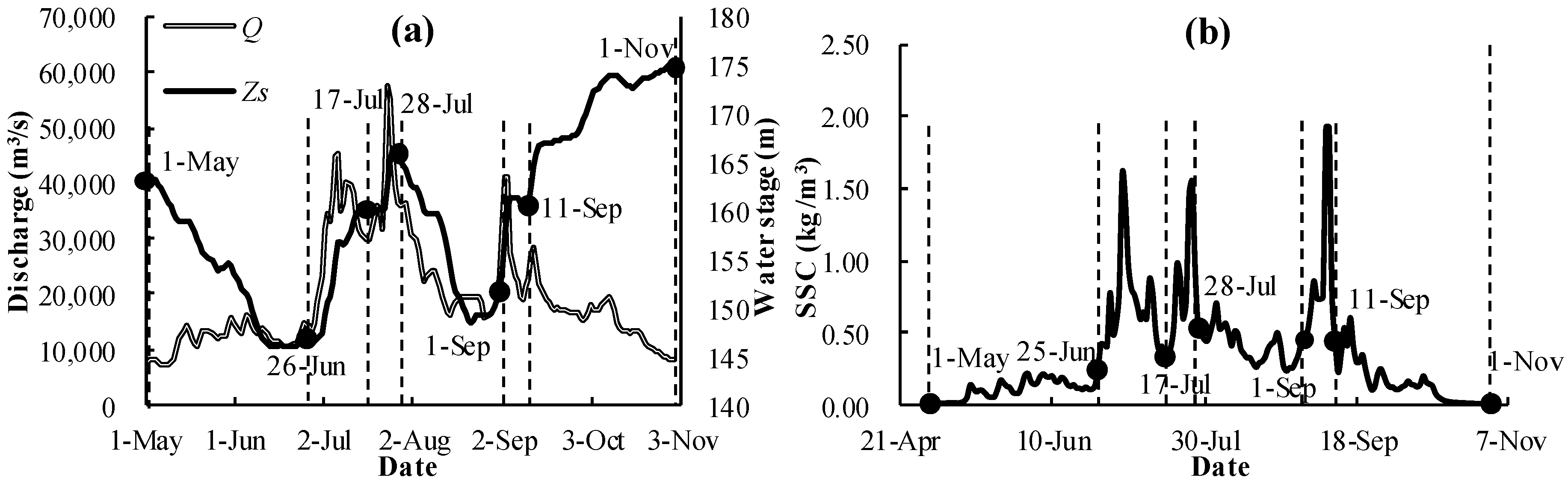
The year 2012 is selected to study the secondary flow effects on bed morphology variation in this reach because of the record amount of deposition that year. The inlet and outlet boundaries are S209 and S201, respectively (Figure 2). The observed flow and sediment discharges at Qingxichang (QXC) and Wanxian (WX) gauging stations have been depicted in Figure 3a,b, respectively. It clearly illustrates that the flow and sediment hydrographs are synchronous with each other at the two stations after the sediment discharges at WX station have been moved forward by one day. Considering the differences of hydrographs between the two stations and the contributions of tributary inflows are small, the interpolation method has been applied to calculate the incoming flow boundary condition at the HHC reach. The incoming suspended sediment concentration (SSC) boundary condition should be calculated through Equation (17). As the distance ratio of QXC-HHC to HHC-WX is equal to the ratio of the amount of deposition at QXC-HHC to that at HHC-WX in 2012, approximately 3:2 [52], and the flow discharges at the two stations are nearly the same, the interpolation method can be applied to approximate the SSC at the inlet boundary as well. The RMSE (Root Mean Square Error) value of the calculated SSC through the above two methods is 0.05 kg/m3, which is acceptable for sediment deposition is negligible when the SSC is less than 0.1 kg/m3. Besides, the SSC propagation is supposed to delay for one day from QXC station to the HHC reach. The water stage measured at Shibaozhai station is used as the outlet boundary condition (Figure 2). Only the flood season from May to November is simulated instead of a whole year because most sediment is transported during this period (Figure 4b), similar to the method applied by Fang and Rodi [53] to study the sedimentation of near dam region after TGP impoundment. This duration has been divided into six periods based on the water stage process (Figure 4a). It should be noted that the water stage rising during the last period of this process is resulted from the operation of TGP and the water stage and bed elevation data are both based on Wusong base level.
where QS = Q × S, kg/s; Q = flow discharge, m3/s; and S = sediment discharge, kg/s; 0.6 and 0.4 represent percentage of amount of sediment deposition at QXC-HHC and HHC-WX, respectively.
A median size of 0.008 mm is used to represent the inflow cohesive sediment composition of this reach [13]. A flood event on 16 July 2012 is chosen as a verification case for this river reach simulation. Table 3 lists parameters and conditions of it. Because the radius to width ratio (r/w) is in the range of 0.8 to 2.0 (Table 3), this river reach belongs to sharply curved bends. The computation domain of the river reach is divided into 211 × 41 grids in longitudinal and transverse directions, with time steps of 1.0 s and 60.0 s for flow and sediment calculation, respectively.
4. Results
The flow simulation results of L, B, and NL models are verified for the discharge of 30,200 m3·s−1, and the model with best performances has been selected. The preferable model L and the reference model N are used to predict cohesive sediment deposition during an annual hydrograph. The basic parameters, such as eddy viscosity coefficient and roughness of flow module, and parameters of sediment module are calibrated in N model first and then applied to the other models.
4.1. Verifications
4.1.1. Flow
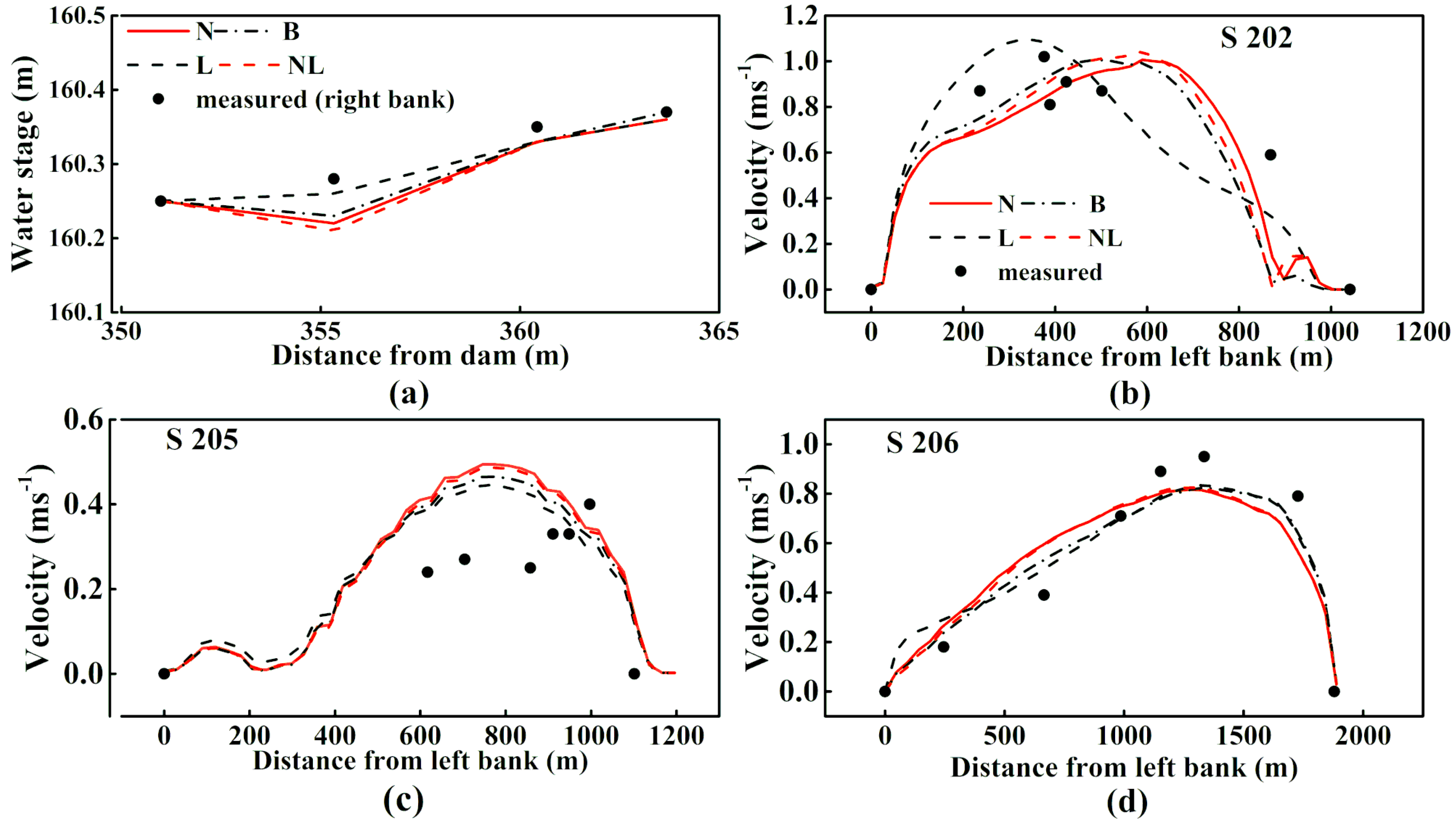
Figure 5 shows simulated water stage at the right bank and the depth-averaged velocities across the channel width of the HHC reach. It can be seen that the results of the L model are more reasonable than those of the other models. The velocity shift due to secondary flow can be well predicted by the L model at the end of the bends (S202 and S206), especially at the exit of the second bend (S202), in contrast to other models. In addition, as the high velocity core shifts to the right bank at the end of the first bend (S206), velocity of the left branches (S205) has been reduced. That explains why the velocities predictions by B and L models are lower than those by N and NL models at S205 (Figure 5c). Overall, the differences among B, N and NL models are small, while the L model is preferable according to the flow simulation results of the HHC reach.
To quantitatively assess the performances of different models in flow simulation of the HHC reach, the RMSE of water stage and velocities of different models at typical cross-sections are listed in Table 4. The L model with the smallest RMSE results outperforms the other models at the discharge of 30,200 m3/s.
4.1.2. Sediment
Based on the above flow simulation results, the L model has been applied to the HHC reach to investigate the secondary flow effects on cohesive sediment deposition. The results of N model serve as references.
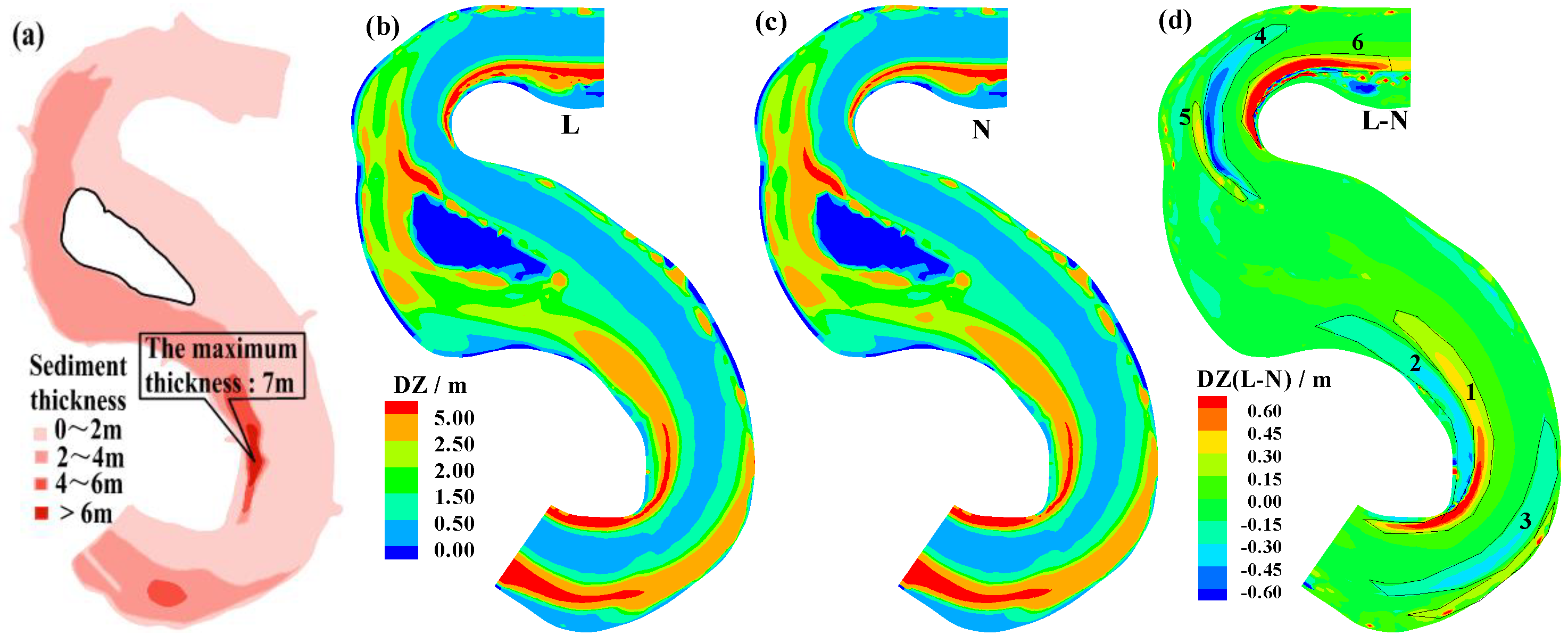
The deposition module is verified by field measurements (Figure 6a) in terms of planar distribution of deposition (Figure 6b,c), bed elevation (Figure 7), and amounts of deposition. Figure 6a–c show that the simulated planar distribution of deposits by the L and N models agree with field measurements qualitatively, with the maximum thickness of deposits found at the convex bank of the first bend, and the majority of deposits located at the right bank of the inlet and the left branch of the reach. The predicted thickness of sediment deposits by the L model is approximately 1 m thicker than that by N model on the concave bank of the first bends (region 1, Figure 6d), which is much closer to the measurement 5–7 m (Figure 6a). Bed elevations simulated by the two models matches well with measurements at S204–S206 (Figure 7). Predictions of total amounts of deposition from S206 to S203 are 8.33 ×10⁶ m3 and 8.0 × 10⁶ m3 by the N and L models respectively, while the field measurement during the same period is 8.18 ×10⁶ m3 [13]. The relative error is around 2%, which qualify the sediment module used in this paper. In general, the L model performs better than the N model in predicting the planar distribution of cohesive sediment deposition.
4.2. Secondary Flow Effects on Cohesive Sediment Deposition
The differences in planar distribution and amounts of deposition predicted by the L and N models have been illustrated in Figure 6d and Figure 8, respectively, which clearly suggest the secondary flow effects on cohesive sediment deposition. Due to its impacts, high velocity core shifts from the convex to the concave bank of the bend, leading to the redistribution of bed shear stress and the consequent morphological changes [9]. Shifts of high velocities predicted by the L model result in the more deposition in region 1, 5, and 6 and less deposition in regions 3 and 4. The increase of sediment deposits in region 1 reduces sediment transported to region 2, resulting in less deposition here. The difference of predicted amount of deposition between the two models is about 0.31 × 10⁶ m3 from 11 September to 1 November, as is clearly shown in Figure 8. This difference is small compared to the total amount of deposition during the whole year, approximately 8.0 × 10⁶ m3. However, this difference can accumulate if the water stage keeps rising due to the impoundment of TGP. In general, secondary flow effects on cohesive sediment deposition become more obvious in the last period of the annual hydrograph when the sediment load is low and water stage is high (Figure 4).
The total deposition volume is calculated from S203–S206 during different periods of this year, because this part of the reach is seldom affected by the inlet and outlet boundaries. Deposition of this part is greatly impacted by the velocity redistribution at S206 (e.g., Figure 5c,d), which is controlled by the secondary flow produced in the upstream bend and the bed topography (transverse bed slope) there. In addition, the sediment load plays an important role in the deposition of this part. Therefore, the average of suspended sediment load during different periods has been shown in Figure 8 as well. When the sediment load is low, the velocity redistribution plays a dominate role resulting in more sediment transport downstream and less deposition due to the shift of high velocities to the right branch. Otherwise, the situation is just reversed, and more deposits can occur in the left branch resulting from the huge amount of sediment transported, despite of the fact that the velocities are higher in the right branch. These can qualitatively explain the difference in predicted amounts of deposition during different periods except the fifth period (1–11 September). In that period, the transverse bed slope at S206 is high enough to strengthen velocity redistribution further, thus surpasses the effects of higher sediment load and result in less predicted deposition by the L model than the N model. During the last period (11 September–1 November), the significant difference of predicted deposition volume is resulted from both the low sediment load transport and the large transverse bed slope.
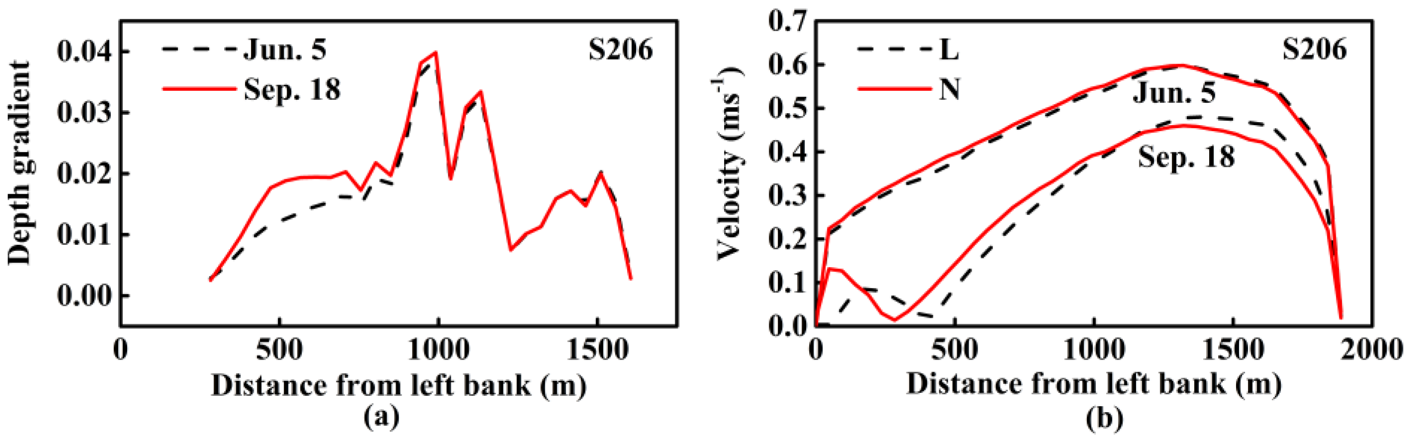
Figure 9 shows the predicted depth gradients (a) and velocity distributions (b) by the L and N models at S206 on 5 June and 18 September (as typical days of the first and last periods), respectively, illustrating the effects of bed topography. It clearly reveals that the velocity redistribution on 18 September is resulted from the bed topography effects as the sediment load on the two days is ~0.1–0.3 kg·m−3. In all, the low sediment load and the velocity redistribution induced by secondary flow produced by upstream bend and the bed topography result in the difference deposition predictions by the two models.
5. Discussion
One of the most important physical processes in meandering rivers is the outward shifting of main flow velocity caused by secondary flow, which is driven by channel curvature or point bars bed topography [3]. The latter one is called topography steering [9], which plays a significant role in meander dynamics [3]. Whether and how the correction terms representing the secondary flow effects quantify this process and the performances of these models in meandering channels of different scales will be discussed in this part. Besides, secondary flow effects on the total amount of deposition of the aforementioned part of this reach (S203–S206) are controlled by the properties of cohesive sediment, which will be investigated as well.
5.1. Secondary Flow Effects on Flow Field
5.1.1. Topography Effects
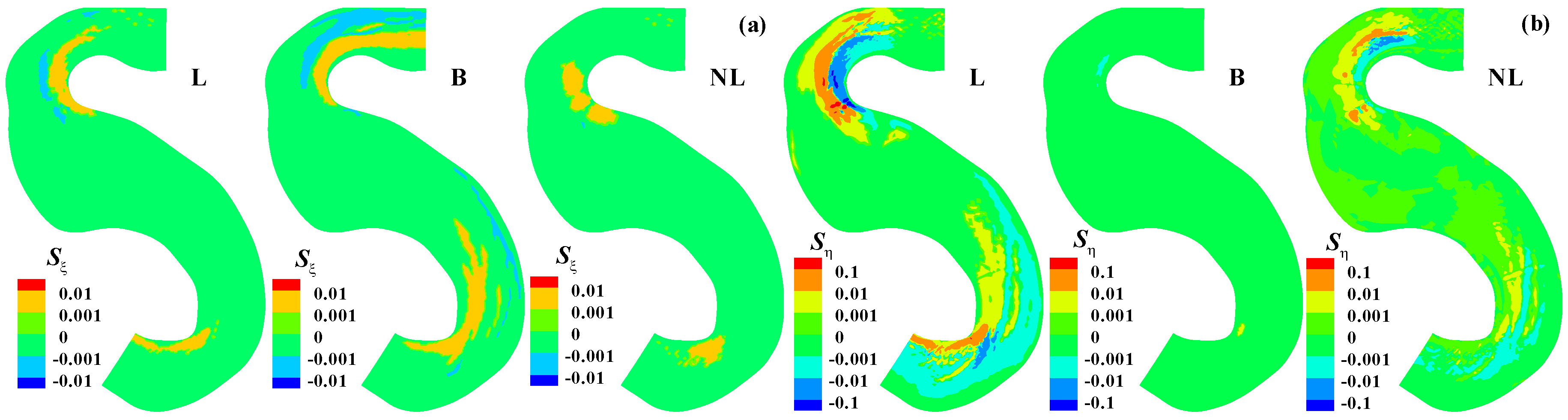
Equation (6) clearly reveals that the correction terms of the three models are directly proportional to the gradients of water depth (H). Due to the effects of bed topography, the longitudinal and transverse gradient of water depth in HHC reach is in the range of 0.01 to 0.001 and 0.01 to 0.1, respectively. Therefore the magnitudes of correction terms follow the same tendency as that of the gradients of water depths, in other words, the correction terms are able to reflect the topography effects. This finding has been justified by Lane [54] who pointed out that correction terms represent the gradients of the transport of momentum. Figure 10 depicts the distributions of (a) Sξ and (b) Sη of the L, B and NL models along the channel. The orders of magnitude of them are within 0.01 to 0.001 in the longitudinal direction, which is the same as the longitudinal gradient of water depth. In the transverse direction, the order of magnitude of the L model is 0.01–0.1, which is consistent with the transverse gradient of water depth, while those of the B and NL models are approaching to zero and in the range of 0.01 to 0.001, respectively. The smaller orders of magnitude of the two models are resulted from the methods of them. As to the B model [35], it only considers the longitudinal correction. As to the NL model [1], the sharpness of the HHC reach limits the growth of the secondary flow. Since the L model considers the corrections in both directions and has larger correction values than the other two models, it outperforms the other models in the flow simulation as shown in Figure 5. In addition, the simulation results shown in Figure 5 clearly indicate that 2D depth-averaged model that include secondary flow effects (e.g., the L and B models) should be given first priority when it comes to sharp meandering channels with bed topography, such as the HHC reach. This has been confirmed by de Vriend [55] who found that his mathematical model with considering secondary flow effects worked better for curved bend flow simulation over developed bed.
5.1.2. Applicability of Different Secondary Flow Models
The differences among these models are listed in Table 1, which mainly lie in whether considering the effects of phase lag (B and NL models), sidewall boundary conditions (B model), and bend sharpness (NL model). As the HHC reach is sharply curved bends, the saturation effect considered by the NL model has weakened the secondary flow effects, which result in the minor differences of simulation results between the NL and N models (Figure 5). The depth to width ratio (H/w) distinguishes between meandering channels of different scales. It is approximately 0.001–0.06 in the HHC reach at the discharge of 30,200 m3/s, while that in the laboratory bend channels and small meandering rivers are in the range of 0.05 to 0.25 [45] and 0.06 to 0.1 [56], respectively. Therefore, the effects of wall boundary conditions and phase lag have been reduced for such small value of H/w. Although B model has taken the bed topography effects into account in a similar way as the L model does, its correction terms only focus on the longitudinal direction. Consequently, the flow simulation results of the L model are better than that of the B model in the HHC reach. Overall, L model is preferable to flow simulation in meandering channels of mega scale, such as HHC reach. However, for laboratory scale curved bends with flat bathymetry, the B model obtains better results [45]. And for sharply curved bends of laboratory and small meandering rivers scales, the advantages of the NL model have been exhibited according to the flow simulation results by Blanckaert [1,2] and Ottevanger [57]. The H/w may play an important role, while the main reasons remain to be further investigated.
5.2. Secondary Flow Effects on Deposition Amounts
According to the deposition simulation results, secondary flow effects on the total deposition volume are small during an annual hydrograph (Figure 8). However, these effects vary with the changes of the cohesive sediment properties, such as settling velocity and critical shear stresses of cohesive sediment, which depend on the flow conditions and the process of bed consolidation. Series of numerical experiments are designed to investigate secondary flow effects on the deposition volume of cohesive sediment with different properties; these effects are reflected by the relative difference in deposition amounts (RD) predicted by the N and L models. Numerical experiments are conducted under the same flow condition (Table 3) to keep the strength of secondary flow constant in the HHC reach. The calculation time for each experiment is 33 days. Different properties of cohesive sediment (Table 5) are represented by the variation of settling velocity (ωs) and the critical shear stress for deposition (τcd). Other parameters used in sediment module are the same as that of HHC reach.
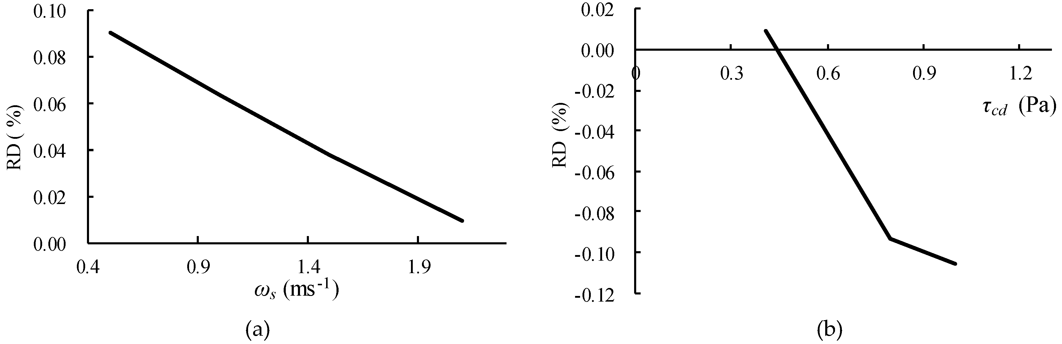
Calculated RD values are listed in Table 5. It is obtained by calculating the difference of the predicted amounts of deposition by L and N models, and then divided by the N model predictions. The negative value of it means the amount of deposition simulated by the L model is smaller than that by the N model. The relationships of RD against ωs and τcd are shown in Figure 11. RD is in reverse linear proportion to ωs, which means the secondary flow effects on the deposition volume increase with the decrease of settling velocity of cohesive sediment. For τcd is ~0.44 Pa, RD is approaching zero. It implies that secondary flow nearly has no effect on the total deposition volume while its effects on planar distribution can still exit (Figure 6d). As the τcd increases, the secondary flow impacts on deposition become greater. In general, RD varies with the settling velocity and critical shear stress for deposition of cohesive sediment and the magnitudes of RD are within 11% based on the parameter values used here.
5.3. Future Reseach Directions
- As the study case is a reach of Yangtze River, which is classed as a mega river, secondary flow effects on bed morphology of meandering channels of different scales (natural rivers with different width to depth ratio) should be investigated. Besides, as the bank of HHC reach is nonerosional, the evolutions of natural rivers with floodplain consisting of cohesive sediment should be simulated by the 2D model developed here. In addition, long-term simulations, such as decadal timescales, should be considered in the future to research the cumulative effects of secondary flow.
- As to the cohesive sediment transport, the values of parameters play important parts in the distributions and amounts of sediment deposition (Figure 11). The roles they played should be compared with that of secondary flow in bed morphology variations. More importantly, the erosion processes should be studied as these processes cannot be reflected obviously in the HHC reach.
6. Conclusions
In order to investigate secondary flow effects on cohesive sediment deposition in a meandering reach of the Yangtze River, a 2D depth-averaged model (N model) has been improved to consider different impacts of secondary flow and cohesive sediment transport. The improved 2D model includes three different submodels, that is, the Lien (L) model [37], with a wide application in literature; the Bernard (B) model [35], considering the phase lag effect and sidewall boundary conditions of secondary flow; and a nonlinear (NL) model [1] accounting for the saturation effect of secondary flow in sharp bends. All of the models can reflect velocity redistribution caused by secondary flow to a certain degree. A module for cohesive sediment transport has been coupled into the N model as well. The simulation results are as follows.
- In flow calculations, the secondary flow effects on water stage and velocity distribution are well predicted. Velocity redistribution has been reproduced fairly well by the L model in the HHC reach, which means the improved 2D depth-averaged model is able to predict the secondary flow impacts on flow field in meandering channels of such mega scale. A previous study by the authors [45] pointed out that the B model is preferable in flow simulations of laboratory meandering channels with flat bathymetry. Further analyses found that secondary flow correction submodels can reflect the bed topography effects and the transverse bed topography, which is neglected by the B model, is more important than the longitudinal one. This explains why the L model performs better than the B model for curved flow simulation over bed topography. In addition, the NL model does not exhibit its advantages in field mega scale meandering reach with high curvatures as that in sharply curved bends of laboratory and small river scales, although the importance of their nonlinear effects on flow simulations have been emphasized by Blanckeart [1,2] and Ottevanger [57]. The reasons need to be further analyzed. In cohesive sediment deposition simulations, the L model performs better than the N model in planar distribution of deposition, due to more sediment deposit on the concave banks of the bends, which is resulted from the velocity redistribution caused by secondary flow.
- The difference in predicted amounts of deposition between the L and N models is evident during the last period of an annual hydrograph when the sediment load is low and the velocity redistribution caused by bed topography is obvious in this reach. This implies that the secondary flow effects on the cohesive sediment deposition vary in an annual hydrography and temporal influence of secondary flow should be considered. This result is similar to that has been found by Guan et al. [28] who conducted a 2D depth-averaged model simulation with secondary flow correction in a natural meandering river dominated by bed load.
- Secondary flow effects on predicted amounts of deposition vary with the settling velocity and critical shear stress for deposition of cohesive sediment, and the relative difference of predicted total amounts of deposition by the L and N models is within 11% based on the parameter values used here.
Author Contributions
Conceptualization, C.Q. and X.S.; methodology, C.Q.; software, C.Q.; validation, C.Q.; formal analysis, C.Q.; investigation, C.Q.; resources, Y.X.; data curation, Y.X.; writing—original draft preparation, C.Q.; writing—review and editing, X.S.; visualization, C.Q.; supervision, X.S.; project administration, X.S.; funding acquisition, X.S.
Funding
This research was funded by the National Key R&D Program of China (2018YFC0407402-01).
Acknowledgments
The authors would like to thank Baozhen Jia for her helpful advice and discussion about this paper and Yanjun Wang for the formation of the ideas about this paper.
Conflicts of Interest
The authors declare no conflict of interest.
References
- Blanckaert, K.; de Vriend, H.J. Nonlinear modeling of mean flow redistribution in curved open channels. Water Resour. Res. 2003, 39. [Google Scholar] [CrossRef]
- Blanckaert, K.; de Vriend, H.J. Meander dynamics: A nonlinear model without curvature restrictions for flow in open-channel bends. J. Geophys. Res. 2010, 115. [Google Scholar] [CrossRef] [Green Version]
- Camporeale, C.; Perona, P.; Porporato, A.; Ridolfi, L. Hierarchy of models for meandering rivers and related morphodynamic processes. Rev. Geophys. 2007, 45. [Google Scholar] [CrossRef] [Green Version]
- Duan, J.G.; Julien, P.Y. Numerical simulation of the inception of channel meandering. Earth Surf. Process. Landf. 2005, 30, 1093–1110. [Google Scholar] [CrossRef]
- Jang, C.-L.; Shimizu, Y. Numerical Simulation of Relatively Wide, Shallow Channels with Erodible Banks. J. Hydraul. Eng. 2005, 131, 565–575. [Google Scholar] [CrossRef] [Green Version]
- Sun, J.; Lin, B.-L.; Kuang, H.-W. Numerical modelling of channel migration with application to laboratory rivers. Int. J. Sediment Res. 2015, 30, 13–27. [Google Scholar] [CrossRef]
- Odgaard, A.J.; Bergs, M.A. Flow Processes in a Curved Alluvial Channel. Water Resour. Res. 1988, 24, 45–56. [Google Scholar] [CrossRef]
- Abad, J.D.; Garcia, M.H. Experiments in a high-amplitude Kinoshita meandering channel: 2. Implications of bend orientation on bed morphodynamics. Water Resour. Res. 2009, 45. [Google Scholar] [CrossRef]
- Dietrich, W.E.; Smith, J.D. Influence of the Point Bar on Flow through Curved Channels. Water Resour. Res. 1983, 19, 1173–1192. [Google Scholar] [CrossRef]
- Elina, K.; Petteri, A.; Matti, V.; Hannu, H.; Juha, H. Spatial and temporal distribution of fluvio-morphological processes on a meander point bar during a flood event. Hydrol. Res. 2013, 44, 1022–1039. [Google Scholar] [CrossRef]
- Li, W.; Wang, J.; Yang, S.; Zhang, P. Determining the Existence of the Fine Sediment Flocculation in the Three Gorges Reservoir. J. Hydraul. Eng. 2015, 141, 05014008. [Google Scholar] [CrossRef]
- Li, W.; Yang, S.; Jiang, H.; Fu, X.; Peng, Z. Field measurements of settling velocities of fine sediments in Three Gorges Reservoir using ADV. Int. J. Sediment Res. 2016, 31, 237–243. [Google Scholar] [CrossRef]
- Xiao, Y.; Yang, F.S.; Su, L.; Li, J.W. Fluvial sedimentation of the permanent backwater zone in the Three Gorges Reservoir, China. Lake Reserv. Manag. 2015, 31, 324–338. [Google Scholar] [CrossRef]
- Krone, R.B. Flume Studies of the Transport of Sediment in Estuarial Shoaling Processes; Hydraulic Engineering Laboratory, University of California: Berkeley, CA, USA, 1962. [Google Scholar]
- De Vriend, H.J. Velocity redistribution in curved rectangular channels. J. Fluid Mech. 1981, 107, 423–439. [Google Scholar] [CrossRef]
- Johannesson, H.; Parker, G. Velocity Redistribution in Meandering Rivers. J. Hydraul. Eng. 1989, 115, 1019–1039. [Google Scholar] [CrossRef]
- Blanckaert, K. Saturation of curvature-induced secondary flow, energy losses, and turbulence in sharp open-channel bends: Laboratory experiments, analysis, and modeling. J. Geophys. Res. 2009, 114. [Google Scholar] [CrossRef] [Green Version]
- Johannesson, H.; Parker, G. Secondary Flow in Mildly Sinuous Channel. J. Hydraul. Eng. 2015, 115, 289–308. [Google Scholar] [CrossRef]
- Nicholas, A.P.; Ashworth, P.J.; Sambrook Smith, G.H.; Sandbach, S.D. Numerical simulation of bar and island morphodynamics in anabranching megarivers. J. Geophys. Res. Earth Surf. 2013, 118, 2019–2044. [Google Scholar] [CrossRef] [Green Version]
- Ashworth, P.J.; Best, J.L.; Roden, J.E.; Bristow, C.S.; Klaassen, G.J. Morphological evolution and dynamics of a large, sand braid-bar, Jamuna River, Bangladesh. Sedimentology 2000, 47, 533–555. [Google Scholar] [CrossRef]
- Hackney, C.R.; Darby, S.E.; Parsons, D.R.; Leyland, J.; Aalto, R.; Nicholas, A.P.; Best, J.L. The influence of flow discharge variations on the morphodynamics of a diffluence-confluence unit on a large river. Earth Surf. Process. Landf. 2018, 43, 349–362. [Google Scholar] [CrossRef]
- Parsons, D.R.; Best, J.L.; Lane, S.N.; Orfeo, O.; Hardy, R.J.; Kostaschuk, R. Form roughness and the absence of secondary flow in a large confluence–diffluence, Rio Paraná, Argentina. Earth Surf. Process. Landf. 2007, 32, 155–162. [Google Scholar] [CrossRef]
- Szupiany, R.N.; Amsler, M.L.; Hernandez, J.; Parsons, D.R.; Best, J.L.; Fornari, E.; Trento, A. Flow fields, bed shear stresses, and suspended bed sediment dynamics in bifurcations of a large river. Water Resour. Res. 2012, 48. [Google Scholar] [CrossRef]
- Szupiany, R.N.; Amsler, M.L.; Parsons, D.R.; Best, J.L. Morphology, flow structure, and suspended bed sediment transport at two large braid-bar confluences. Water Resour. Res. 2009, 45. [Google Scholar] [CrossRef] [Green Version]
- Nicholas, A.P. Modelling the continuum of river channel patterns. Earth Surf. Process. Landf. 2013, 38, 1187–1196. [Google Scholar] [CrossRef]
- Rhoads, B.L.; Johnson, K.K. Three-dimensional flow structure, morphodynamics, suspended sediment, and thermal mixing at an asymmetrical river confluence of a straight tributary and curving main channel. Geomorphology 2018, 323, 51–69. [Google Scholar] [CrossRef]
- Abad, J.D.; Buscaglia, G.C.; Garcia, M.H. 2D stream hydrodynamic, sediment transport and bed morphology model for engineering applications. Hydrol. Process. 2008, 22, 1443–1459. [Google Scholar] [CrossRef]
- Guan, M.; Wright, N.G.; Sleigh, P.A.; Ahilan, S.; Lamb, R. Physical complexity to model morphological changes at a natural channel bend. Water Resour. Res. 2016, 52, 6348–6364. [Google Scholar] [CrossRef] [Green Version]
- Iwasaki, T.; Shimizu, Y.; Kimura, I. Sensitivity of free bar morphology in rivers to secondary flow modeling: Linear stability analysis and numerical simulation. Adv. Water Resour. 2016, 92, 57–72. [Google Scholar] [CrossRef]
- Yang, H.; Lin, B.; Sun, J.; Huang, G. Simulating Laboratory Braided Rivers with Bed-Load Sediment Transport. Water 2017, 9, 686. [Google Scholar] [CrossRef]
- Kasvi, E.; Alho, P.; Lotsari, E.; Wang, Y.; Kukko, A.; Hyyppä, H.; Hyyppä, J. Two-dimensional and three-dimensional computational models in hydrodynamic and morphodynamic reconstructions of a river bend: Sensitivity and functionality. Hydrol. Process. 2015, 29, 1604–1629. [Google Scholar] [CrossRef]
- Kang, T.; Kimura, I.; Shimizu, Y. Responses of Bed Morphology to Vegetation Growth and Flood Discharge at a Sharp River Bend. Water 2018, 10, 223. [Google Scholar] [CrossRef]
- Reesink, A.J.H.; Ashworth, P.J.; Sambrook Smith, G.H.; Best, J.L.; Parsons, D.R.; Amsler, M.L.; Hardy, R.J.; Lane, S.N.; Nicholas, A.P.; Orfeo, O.; et al. Scales and causes of heterogeneity in bars in a large multi-channel river: Río Paraná, Argentina. Sedimentology 2014, 61, 1055–1085. [Google Scholar] [CrossRef]
- Begnudelli, L.; Valiani, A.; Sanders, B.F. A balanced treatment of secondary currents, turbulence and dispersion in a depth-integrated hydrodynamic and bed deformation model for channel bends. Adv. Water Resour. 2010, 33, 17–33. [Google Scholar] [CrossRef]
- Bernard, R.S. STREMR: Numerical Model for Depth-Averaged Incompressible Flow; Hydraulics Laboratory (Waterways Experiment Station), U.S. Army Corps of Engineers: Vicksburg, MS, USA, 1993.
- Duan, J.G. Simulation of Flow and Mass Dispersion in Meandering Channels. J. Hydraul. Eng. 2004, 130, 964–976. [Google Scholar] [CrossRef]
- Lien, H.C.; Hsieh, T.Y.; Yang, J.C.; Yeh, K.C. Bend-Flow Simulation Using 2D Depth-Averaged Model. J. Hydraul. Eng. 1999, 125, 1097–1108. [Google Scholar] [CrossRef]
- Song, C.G.; Seo, I.W.; Kim, Y.D. Analysis of secondary current effect in the modeling of shallow flow in open channels. Adv. Water Resour. 2012, 41, 29–48. [Google Scholar] [CrossRef]
- Jin, Y.-C.; Steffler, P.M. Predicting Flow in Curved Open Channels by Depth-Averaged Method. J. Hydraul. Eng. 1993, 119, 109–124. [Google Scholar] [CrossRef]
- Abad, J.D.; Garcia, M.H. Experiments in a high-amplitude Kinoshita meandering channel: 1. Implications of bend orientation on mean and turbulent flow structure. Water Resour. Res. 2009, 45. [Google Scholar] [CrossRef] [Green Version]
- Wu, W.; Wang, S.Y. Depth-Averaged 2-D Calculation of Flow and Sediment Transport in Curved Channels. Int. J. Sediment Res. 2004, 19, 241–257. [Google Scholar]
- Wang, H.; Zhou, G.; Shao, X. Numerical simulation of channel pattern changes Part I: Mathematical model. Int. J. Sediment Res. 2010, 25, 366–379. [Google Scholar] [CrossRef]
- WL|DelftHydraulics. Delft3D-FLOW User Manual (Version: 3.15.30059): Simulation of Multi-Dimensional Hydrodynamic Flows and Transport Phenomena, Including Sediments; Deltares: Rotterdamseweg, The Netherlands, 2013; pp. 226–230. [Google Scholar]
- Hosoda, T.; Nagata, N.; Kimura, I.; Michibata, K.; Iwata, M. A Depth Averaged Model of Open Channel Flows with Lag between Main Flows and Secondary Currents in a Generlized Curvilinear Coordinate System. In Proceedings of the Advances in Fluid Modeling and Turbulence Measurements, Tokyo, Japan, 4–6 December 2001; pp. 63–70. [Google Scholar]
- Qin, C.; Shao, X.; Zhou, G. Comparison of Two Different Secondary Flow Correction Models for Depth-averaged Flow Simulation of Meandering Channels. Procedia Eng. 2016, 154, 412–419. [Google Scholar] [CrossRef] [Green Version]
- Ottevanger, W. Modelling and Parameterizing the Hydro-and Morphodynamics of Curved Open Channels. Ph.D. Thesis, Delft University of Technology, Delft, The Netherlands, 2013. [Google Scholar]
- Gu, L.; Zhang, S.; He, L.; Chen, D.; Blanckaert, K.; Ottevanger, W.; Zhang, Y. Modeling Flow Pattern and Evolution of Meandering Channels with a Nonlinear Model. Water 2016, 8, 418. [Google Scholar] [CrossRef]
- Lin, Q.; Wu, W. A one-dimensional model of mixed cohesive and non-cohesive sediment transport in open channels. J. Hydraul. Res. 2013, 51, 506–517. [Google Scholar] [CrossRef]
- Latrubesse, E.M. Large rivers, megafans and other Quaternary avulsive fluvial systems: A potential “who’s who” in the geological record. Earth-Sci. Rev. 2015, 146, 1–30. [Google Scholar] [CrossRef]
- Dargahi, B. Three-dimensional flow modelling and sediment transport in the River Klarälven. Earth Surf. Process. Landf. 2004, 29, 821–852. [Google Scholar] [CrossRef]
- Kleinhans, M.G.; Jagers, H.R.A.; Mosselman, E.; Sloff, C.J. Bifurcation dynamics and avulsion duration in meandering rivers by one-dimensional and three-dimensional models. Water Resour. Res. 2008, 44. [Google Scholar] [CrossRef]
- YRWC. Analyses of Flow-Sediment Characteristics, the Reservoir Siltation and the River Erosion in the Lower Reaches of the Three Gorges Reservoir in 2012; Yangtze Water Resources Commission: Wuhan, China, 2013.
- Fang, H.-W.; Rodi, W. Three-dimensional calculations of flow and suspended sediment transport in the neighborhood of the dam for the Three Gorges Project (TGP) reservoir in the Yangtze River. J. Hydraul. Res. 2010, 41, 379–394. [Google Scholar] [CrossRef]
- Lane, S.N. Hydraulic modelling in hydrology and geomorphology: A review of high resolution approaches. Hydrol. Process. 2015, 12, 1131–1150. [Google Scholar] [CrossRef]
- De Vriend, H.J. A Mathematical Model Of Steady Flow In Curved Shallow Channels. J. Hydraul. Res. 1977, 15, 37–54. [Google Scholar] [CrossRef]
- Miao, W.; Blanckaert, K.; Heyman, J.; Li, D.; Schleiss, A.J. A parametrical study on secondary flow in sharp open-channel bends: Experiments and theoretical modelling. J. Hydro-Environ. Res. 2016, 13, 1–13. [Google Scholar]
- Ottevanger, W.; Blanckaert, K.; Uijttewaal, W.S.J. Processes governing the flow redistribution in sharp river bends. Geomorphology 2012, 163–164, 45–55. [Google Scholar] [CrossRef]
Figure 1.
Solution procedure.

Figure 2.
Planform geometry, bed elevation (Z0) on March 2012 and nine cross-sections measured in HHC reach (S209 and S201 are the inlet and outlet boundaries, respectively; incoming flow discharge and sediment concentration used as inlet boundaries are interpolated from Qingxichang and Wanxian gauging station, located upstream 476.46 km and 291.38 km from TGP, respectively; and the outlet boundary applies the water stage measured at Shibaozhai station, located upstream 341.35 km from the TGP).

Figure 3.
(a) Hydrograph at Qingxichang (QXC) and Wanxian (WX) gauging stations. (b) Sediment discharge (QS) measured at QXC and WX and calculated at HHC (The QS at WX station has been moved forward by one day).
Figure 3.
(a) Hydrograph at Qingxichang (QXC) and Wanxian (WX) gauging stations. (b) Sediment discharge (QS) measured at QXC and WX and calculated at HHC (The QS at WX station has been moved forward by one day).

Figure 4.
(a) Hydrograph and water stage from May 1 to November 1 (Q and ZS represent discharge and water stage, respectively); the black filled circles divide the duration into several periods descripted clearly by the vertical black dash lines. (b) Suspended sediment concentration (SSC) as the inlet boundary in this duration.

Figure 5.
(a) Water stage of the right bank (downstream view). (b–d) Depth-averaged velocity distribution measured and predicted by N, B, L, and NL models at three cross-sections for discharge 30,200 m3/s.
Figure 5.
(a) Water stage of the right bank (downstream view). (b–d) Depth-averaged velocity distribution measured and predicted by N, B, L, and NL models at three cross-sections for discharge 30,200 m3/s.

Figure 6.
(a) Planar distribution of sediment thickness measured, the maximum is 7 m from March to August, 2012. (b) Sediment thickness simulated by the L model (c) and N model. (d) The difference between the L and N models.
Figure 6.
(a) Planar distribution of sediment thickness measured, the maximum is 7 m from March to August, 2012. (b) Sediment thickness simulated by the L model (c) and N model. (d) The difference between the L and N models.

Figure 7.
Comparison of bed elevation at cross-sections between measurements and predictions.

Figure 8.
Differences in deposition volume during different periods (average SSC means the average suspended sediment concentration during each period).
Figure 8.
Differences in deposition volume during different periods (average SSC means the average suspended sediment concentration during each period).

Figure 9.
(a) Depth gradient (represents bed topography effects). (b) Velocity distribution predicted by the N and L models at S206 on typical days of the first and last period, respectively.
Figure 9.
(a) Depth gradient (represents bed topography effects). (b) Velocity distribution predicted by the N and L models at S206 on typical days of the first and last period, respectively.

Figure 10.
Correction terms (a) Sξ and (b) Sη distributions of the L, B, and NL models along the channel.
Figure 10.
Correction terms (a) Sξ and (b) Sη distributions of the L, B, and NL models along the channel.

Figure 11.
The relationships of relative difference in deposition volume (RD) predicted by the L and N models against (a) settling velocity (ωs) and (b) critical shear stress (τcd).
Figure 11.
The relationships of relative difference in deposition volume (RD) predicted by the L and N models against (a) settling velocity (ωs) and (b) critical shear stress (τcd).


Table 1.
Differences between L, B, and NL models.
| L Model | B Model | NL Model | |
|---|---|---|---|
| Saturation effect | NO | NO | YES |
| Phase lag effect | NO | YES | YES |
| Wall boundary condition | - | no secondary flow produced | dispersion terms = 0 |
| Velocity redistribution | YES | YES | YES |
Table 2.
Model parameters used for cohesive sediment calculation.
| Related Variables | Values |
|---|---|
| Settling velocity ωs | 2.1 mm·s−1 |
| Critical shear stresses τcd, τce Erosion coefficient M Empirical coefficient n | 0.41 Pa 1.0 × 10⁻⁸ kg·m−2·s−1 2.5 |
Table 3.
Channel dimensions and flow condition of HHC reach.
| Study Case | Discharge Q (m3 s−1) | Depth H (m) | Width w (km) | Bend Radius r (km) | r/w | H/r | Adaption Length λ |
|---|---|---|---|---|---|---|---|
| HHC | 30,200 | 16–67 | 0.7–2.0 | >0.4 | 0.8–2.0 | 0.001–0.066 | 0.001–0.2 |
Table 4.
The RMSE of water stage (rows 1–3) and velocities (rows 4–9) of different models.
| RMSE | N | L | B | NL |
|---|---|---|---|---|
| Left bank | 0.049 | 0.049 | 0.054 | 0.051 |
| Right bank | 0.032 | 0.015 | 0.027 | 0.037 |
| Mean | 0.041 | 0.037 | 0.043 | 0.045 |
| S202 | 0.204 | 0.173 | 0.242 | 0.252 |
| S203 | 0.243 | 0.249 | 0.236 | 0.233 |
| S204 | 0.127 | 0.093 | 0.112 | 0.120 |
| S205 | 0.151 | 0.121 | 0.133 | 0.145 |
| S206 | 0.147 | 0.110 | 0.111 | 0.142 |
| Mean | 0.179 | 0.160 | 0.177 | 0.186 |
Table 5.
Settling velocity (ωs) and critical shear stress for deposition (τcd) in numerical experiments and results.
Table 5.
Settling velocity (ωs) and critical shear stress for deposition (τcd) in numerical experiments and results.
| ωs (m/s) | RD 1 (%) | τcd (Pa) | RD 1 (%) |
|---|---|---|---|
| 2.1 | 0.92 | 0.41 | 0.92 |
| 1.5 | 3.80 | 0.44 | 0.03 |
| 1.0 | 6.38 | 0.80 | −9.36 |
| 0.5 | 9.01 | 1.00 | −10.61 |
1 The relative difference in deposition amounts (RD) predicted by N and L models.
© 2019 by the authors. Licensee MDPI, Basel, Switzerland. This article is an open access article distributed under the terms and conditions of the Creative Commons Attribution (CC BY) license (http://creativecommons.org/licenses/by/4.0/).
Share and Cite
MDPI and ACS Style
Qin, C.; Shao, X.; Xiao, Y. Secondary Flow Effects on Deposition of Cohesive Sediment in a Meandering Reach of Yangtze River. Water 2019, 11, 1444. https://doi.org/10.3390/w11071444
AMA Style
Qin C, Shao X, Xiao Y. Secondary Flow Effects on Deposition of Cohesive Sediment in a Meandering Reach of Yangtze River. Water. 2019; 11(7):1444. https://doi.org/10.3390/w11071444
Chicago/Turabian StyleQin, Cuicui, Xuejun Shao, and Yi Xiao. 2019. "Secondary Flow Effects on Deposition of Cohesive Sediment in a Meandering Reach of Yangtze River" Water 11, no. 7: 1444. https://doi.org/10.3390/w11071444
Note that from the first issue of 2016, this journal uses article numbers instead of page numbers. See further details here.