Identifying Climate and Human Impact Trends in Streamflow: A Case Study in Uruguay


1
National Research Program on Production and Environmental Sustainability, National Institute of Agricultural Research of Uruguay, 90200 Rincón del Colorado, Departamento de Canelones, Uruguay
2
Institute of Fluid Mechanics and Environmental Engineering, School of Engineering, Universidad de la República, 11200 Montevideo, Departamento de Montevideo, Uruguay
3
School of Life and Environmental Sciences, The University of Sydney, Sydney, NSW 2006, Australia
*
Author to whom correspondence should be addressed.
Water 2019, 11(7), 1433; https://doi.org/10.3390/w11071433
Submission received: 17 June 2019
/
Revised: 6 July 2019
/
Accepted: 9 July 2019
/
Published: 12 July 2019
(This article belongs to the Special Issue Impacts of Climate Change and Anthropogenic Activities on the Spatio-Temporal Variability of River Flow)
Abstract
:Land use change is an important driver of trends in streamflow. However, the effects are often difficult to disentangle from climate effects. The aim of this paper is to demonstrate that trends in streamflow can be identified by analysing residuals of rainfall-runoff simulations using a Generalized Additive Mixed Model. This assumes that the rainfall-runoff model removes the average climate forcing from streamflow. The case study involves the Santa Lucía river (Uruguay), the GR4J rainfall-runoff model, three nested catchments ranging from 690 to 4900 km and 35 years of observations (1981–2016). Two exogenous variables were considered to influence the streamflow. Using satellite data, growth in forest cover was identified, while the growth in water licenses was obtained from the water authority. Depending on the catchment, effects of land use change differ, with the largest catchment most impacted by afforestation, while the middle size catchment was more influenced by the growth in water licenses.
1. Introduction
Global water resources are limited and under pressure across the world [1]. The total amount of water that can be used for irrigation, water supply or power generation is defined by the transfer of moisture between climate and landscape [2]. The effect of climate on water resources is often concealed because the processes in the landscape are changing [3,4].
There have been a number of recent publications identifying the combined impact on water resources of land use change and climate change and variability (e.g., [5,6,7,8]). However, the identification of land-use trends is difficult due to the effect of the overlying climate trends and variability [5,8]. As a result, disentangling the different impacts on streamflow is not an easy task, particularly since it is ver difficult to perform paired catchment studies, or before and after studies, at regional scales [5]. Several papers have specifically indicated a positive relationship between changes in forest cover and streamflow [5,6,8]. These results appear to be reflected in Uruguay, where afforestation is suggested to cause a reduction in runoff volumes and peak flows [9,10]. But climate variability, especially the El Niño Southern Oscillation, also impacts flow volumes in the south American region [11,12,13], and this would need to be accounted for.
Essentially, identifying the impact of land use change on streamflow can be approached in two different ways. The first is through paired catchment studies (i.e., [9]), but this tends to be unmanageable for larger catchments and is difficult in low data environments. The second option is through time trend analysis (i.e., [5]). Over time, several different statistical techniques have been developed for time trend detection, examples of which are the Mann-Kendall [14,15] and Pettitt test [16]. These two techniques (Mann-Kendall and Pettitt) are popular non-parametric tests used for detecting slowly-varying as well as abrupt changes [17,18,19,20]. Trend analysis can be performed under the assumption of nonstationarity, where variables are detrended into two or more components before analysis, or it can be performed by scaling the hydrological process to model the trend as a stochastic component (and assuming stationarity) [21]. An alternative to classical trend analysis, such as Mann Kendall, is the use of Generalized Additive Mixed Modeling (GAMM) [22,23], which deals with missing data and/or irregularly spaced samples in time. The mixed modelling addition means that the model is also better suited to analysing autocorrelated data. In addition, GAMM models can incorporate multiple variables and identify the importance of different variables included in the overall trend model.
Despite a plethora of techniques, it can still be difficult to identify trends. Some work has suggested identifying non-stationary parameters in models to reflect land use change [24]. However, recently, Serinaldi et al. [25], highlighted that statistical analyses of trends can only offer an indication of a trend or non-stationarity, as many of the analyses are dependent on the length of data and the analysis performed. In addition, Serinaldi et al. [25] warn against using a non-stationary approach, as it is difficult to assess whether a data series is truly non-stationary. Without a supporting physical theory or data, trends can therefore never be fully confirmed, which is a challenge in low data environments.
The motivation for this work is twofold, the first is methodological. As the classic time trend analysis can be problematic [25], this study proposes a different approach, which combines rainfall-runoff modelling with a GAMM regression modelling of the residuals to specifically identify the drivers of trends. The second motivation is regional, past studies in the region have only compared the runoff response to similar rainfall events, before and after land use change [10], and compared landuse effects using paired catchments [9]. The problem with these prior studies is that the approach is difficult to extrapolate to other catchments in the region, and it does not eliminate the effect of climate variability, which this study addresses.
In general, optimizing parameters for a climate forced rainfall-runoff model to a flow data series will result in the average optimized effect of the climate forcing on the streamflow series, as the model cannot fit any trend that is not conceptualized in the model [21]. This suggests that the residuals of a rainfall-runoff model reflect any exogenous trends not reflected in the model. The aim of this paper is therefore to demonstrate for a case study catchment the use of GAMM modelling on the residuals of a climate forced rainfall-runoff model. More specifically, we will use GAMM in a relatively low data environment to identify: (1) do the residuals of the rainfall-runoff model contain remaining seasonal and global trends? (2) can additional trends due to land use change impacts be identified in the residuals from simple time series?
2. Study Area and Dataset
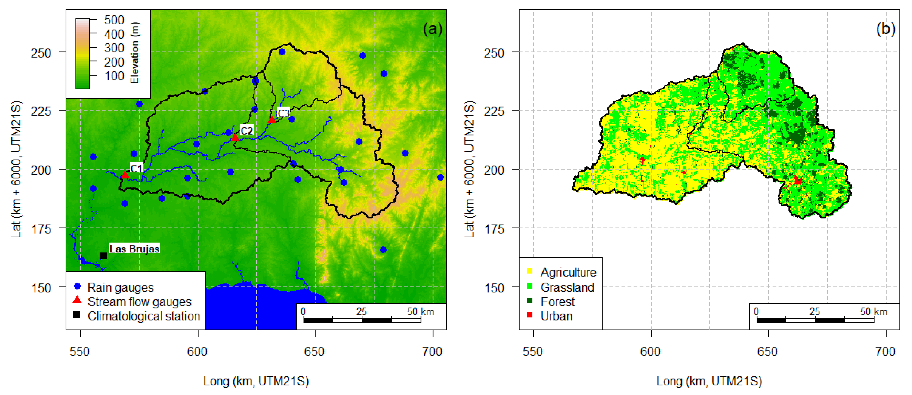
The Santa Lucía catchment is the main source of drinking water for Uruguay. It delivers water for 1.6 million people (about 60% of the population) and supports several agro-industrial activities. In this study we focus specifically on the Santa Lucia at Paso Pache gauging station and the subsequent upstream gauged sites. This area drains a sub-catchment of Santa Lucia with a relatively rich hydrometeorological network (28 rain gauges, 3 stream gauges and 1 climatological station, Figure 1). For the study, the Paso Pache catchment is conceptualized as three nested catchments located at local gauging sites: Catchment 1 (C1), is the largest catchment defined at Paso Pache (4896 km2); Catchment 2 (C2), is the mid-size catchment which drains to Fray Marcos station (2744 km2), upstream from Paso Pache; Catchment 3 (C3), is the smallest catchment limited at Paso de los Troncos (687 km2), upstream from Fray Marcos.
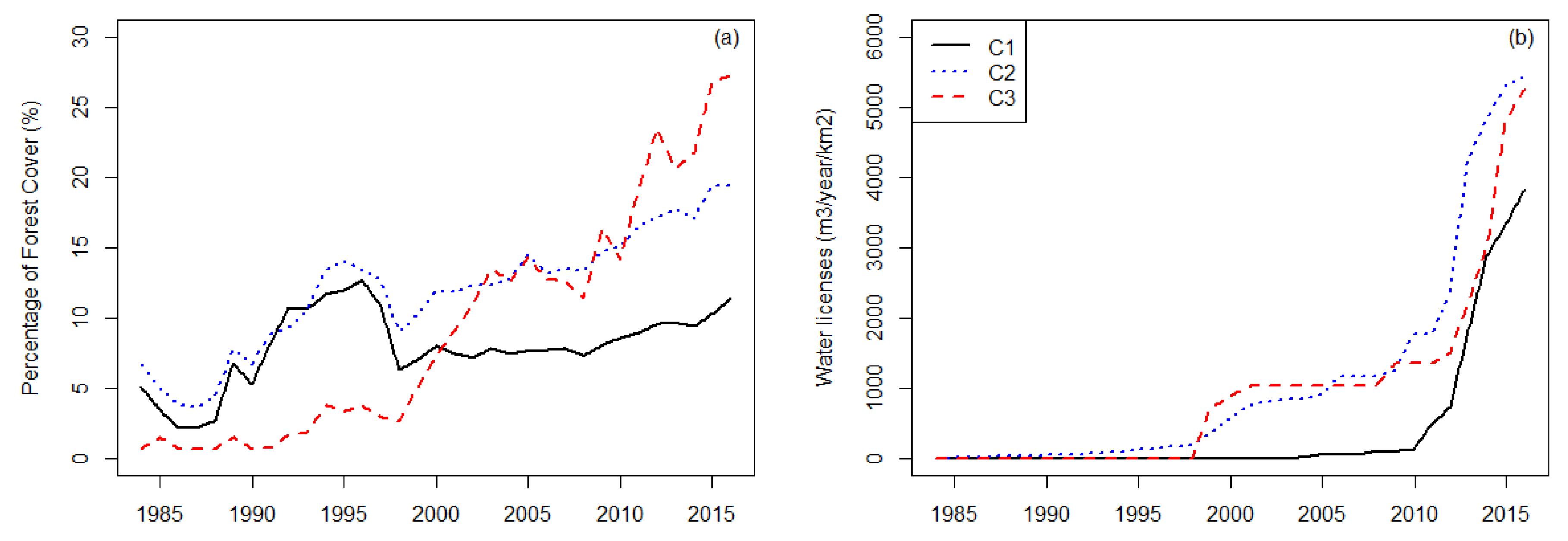
The elevation profile of Paso Pache is characterized by rolling landscape and plains (Figure 1a). The soils are developed from silt and clay from Cretaceous formations, resulting in shallow soils with low water storage capacity. In 2015, the main land use was grassland (54%), followed by small grains and row crop agriculture (34%), forestry (Eucalyptus, 9%), and urban areas (3%) (Figure 1b). However, the forestry and agriculture sectors have changed considerably over the last 30 years: the percentage of forest cover has increased substantially (Figure 2a, based on Google Earth imagery and forest cover classification from the visible images; and the local water authority (DINAGUA, Dirección Nacional de Aguas) has increasingly provided water allocations mainly for irrigation, livestock and domestic (Figure 2b).
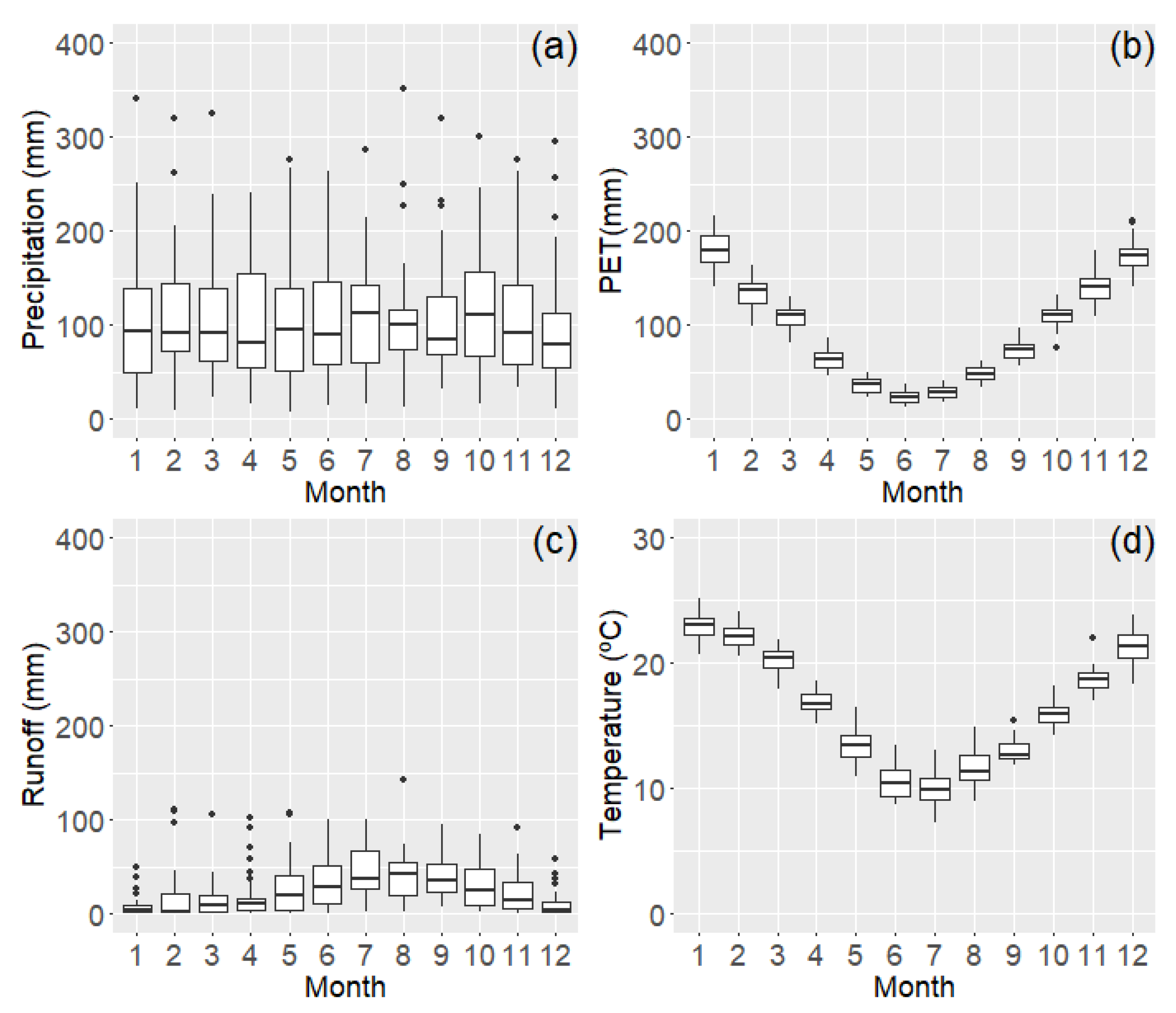
The annual average precipitation is around 1300 mm. The monthly mean precipitation is fairly uniform over the year but with substantial interannual variability (i.e., there is no rainy season but there may be dry or wet years, Figure 3a). Potential evapotranspiration follows temperature, and it reaches a minimum during May–June–July (winter in the southern hemisphere, Figure 3b), and as a result monthly runoff is highest between June and October (Figure 3c).
3. Methodology
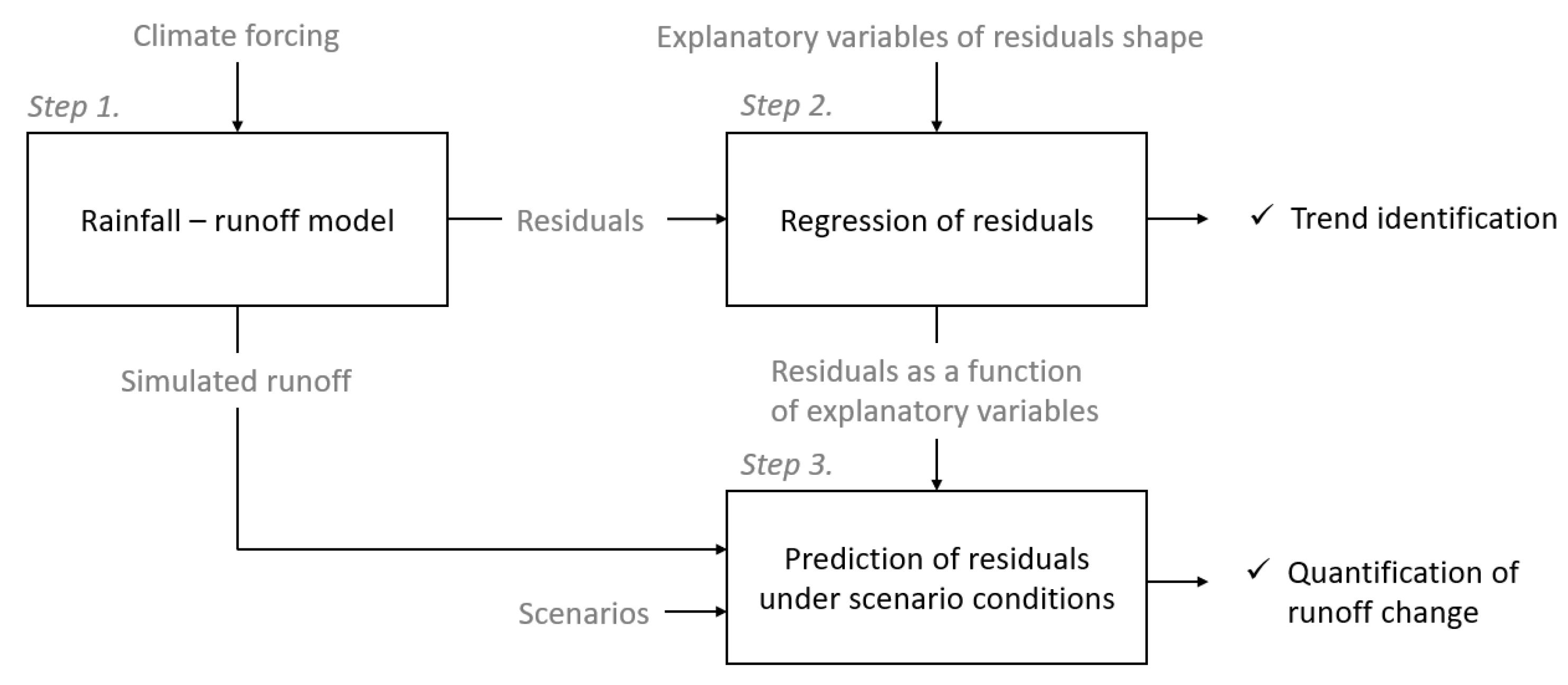
For this study, land use change is hypothesized to create a change in the rainfall-runoff response of a catchment. Figure 4 shows a schematic representation of the proposed method. A climate forced and calibrated rainfall-runoff model should remove the variation in the streamflow due to ‘normal’ year-to-year and seasonal climate variability (Figure 4, step 1). As a result, this will amplify the effect of anthropogenic activities such as afforestation and water allocations in the residual series. Therefore, a trend analysis on the residual series of stationary rainfall-runoff model (Figure 4, step 2), should identify a remaining “global” trend (being long-term increasing or decreasing trend) or a seasonal trend (being a seasonal cycle) in the runoff behavior more easily than using the original series (aim 1). Finally, the runoff change is quantified using the relationships from step 2 using a model stationarity, outlined in Section 3.3 (Figure 4, step 3). Another way to express this is that we use the rainfall-runoff model to remove climate variation in the streamflow and to amplify any remaining trends.
Subsequently, the remaining residual series can still include an unaccounted global and seasonal trend (for example, a seasonal trend due to an interaction of forcing variables on vegetation, such as crop growth). Removing any remaining global and seasonal trends, the effect of afforestation and water allocations would be more easily identified in the series (aim 2). In this section, we describe the rainfall-runoff model and the GAMM models used for trend analysis of the rainfall-runoff model residuals.
3.1. Rainfall-Runoff Simulation
The GR4J model was selected for the rainfall-runoff simulations. GR4J is a daily lumped hydrologic model using precipitation and evapotranspiration as climatological forcing [26]. GR4J has four parameters: capacity of the production store (X1, mm), underground flow exchange coefficient (X2 mm/day), capacity of routing store (X3, mm), and time base for the unit hydrograph (X4, days). Due to its simplicity, this model has been widely used in several landscapes for different purposes [27,28,29]. It is available in the AirGR [30] and hydromad (Andrews et al., 2011) packages for R software [31]. Here, the hydromad implementation of the model was used (http://hydromad.catchment.org/). This package offers a variety of tools to handle data, optimize models, and to analyse and visualize results.
This study used the lumped structure of GR4J without spatial implementation across sub-catchments. The three individual nested gauging sites were used for calibration of the lumped simulation (Figure 1a), offering three simulation scenarios defined by the catchment scales. As a precipitation forcing, the mean areal precipitation of each catchment was estimated based on kriging of the individual rainfall stations by a spherical variogram using the gstat R package [32,33]. In the absence of an evapotranspiration network, the data from the Las Brujas climatological station, located 80 km southwest of the center of the study area, was used (562025 W, 344017 S) to estimate the Penman-Monteith potential evapotranspiration. Based on this, homogeneous potential evapotranspiration was assumed for the region.
The hydromad package offers a variety of assessment and objective functions such as the mean absolute error, root mean squared error, and Nash-Sutcliffe efficiency. For this study a combination of R Squared using square-root transformed daily data and the R Squared aggregated at monthly time steps was used as the objective function [34]. This choice is made to balance the fit to the average flow behavior with the daily variation across all flow regimes [35]. The first year (1981) is defined as the warm-up period and the model is fitted to 1982–2016 using the least squares Nelder-Mead optimisation. To assess the performance of the model calibrations, the skill of GR4J was evaluated at monthly scale after aggregate daily runoff simulations. No validation was performed, as GR4J is only used to remove the climate effects from the data series, assuming that the model fit on the series captures the “average” climate forcing behaviour.
3.2. Trend Simulation of Runoff Residuals
Generalized Additive Mixed Modeling (GAMM) [23] was used to identify trends in the runoff residuals (Qres). The advantage of using GAMM is that this allows very flexible and non-linear regression modelling, something which is not possible with standard linear regression. The GAMM modelling analysed the residuals aggregated to a monthly scale. Qres is defined as the difference between simulated runoff (Qsim) and observed runoff (Qobs) at a monthly scale. The aggregation to the monthly time step is firstly to simplify the management of autocorrelation in the model to a basic first order autocorrelation and secondly to speed-up the GAMM computations. Subsequently, the residuals are log transformed to relative residuals (, Equation (1)) to stabilize the GAMM residual variance as the monthly GR4J residuals have a highly skewed distribution.
In Equation (1), the constant 1 is added to avoid negative values within the logarithmic operator. A key element of GAMM modelling is the use of smooth functions applied to the variables to allow nonlinear modelling. However, this increases the risk of overfitting. The approach in this study is to consider several linear and nonlinear explanatory variables as the relationship between predictand and predictors cannot be known a-priori (Table 1).
In Table 1, G represents an unspecified global trend, and is defined simply as 1 to 442 (which is the total number of months). S describes the seasonal behavior and is defined as month within each year (ranging from 1 to 12). is the Forest Cover as the percentage of surface used for forestry from Figure 2a (age of the forest has not been taken into account). In absence of information about water allocations, the number of Water Licenses (, m3/year/km2) provided by DINAGUA is used (Figure 2b). Finally, the operator indicates a linear operator and indicates a polynomial smooth function. The letters “L” and “S” in the model Id indicates whether is modelled by a linear or a smooth function for G, respectively. In this case we used the cubic shrinkage spline [23] for the smooth functions. Additionally, to restrict the flexibility of the splines, the number of “knots” (k) in the spline was limited to a relatively small value (3). Both the shrinkage spline and the low number of knots reduces the risk of overfitting the model.
To compare the different regression models we focus on the adjusted r2 as a performance measure as this is directly related to the variance explained in the data. The adjusted r2 is a penalised version of the r2 taking into account the number of parameters in the model:
Here n is the number of data points, p is the number of parameters in the model, and y is the response variable.
3.3. Quantifying the Effect of Land Use Change and Water Licenses on Streamflow
To quantify the effect of land use change is a two-step process: (1) Estimation of a new time series related to the desired scenario (). represent the residuals of rainfall runoff-model without the impact of a specific land use change. This involves individually setting the variable and to zero and using the best performing GAMM model to predict streamflow (with and/or ), and the same S and G to generate . (2) The new time series of runoff without the specific land use change is calculated based on the original Qsim. This hypothesizes that the change in land use would have negligible effect on the original GR4J calibration. Thus, the new runoff from the scenario () is computed by Equation (3):
4. Results
4.1. Rainfall-Runoff Model Performance
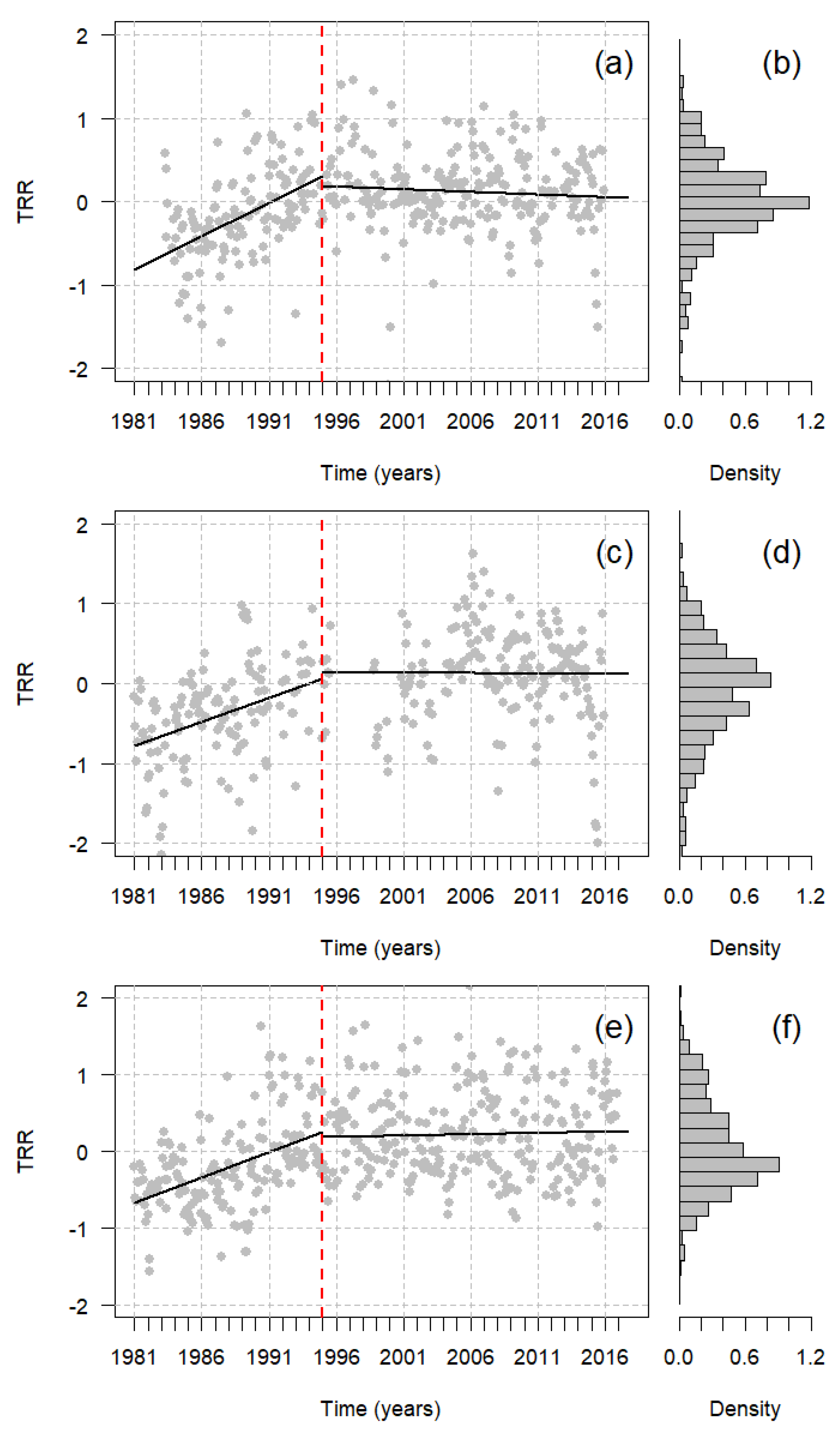
The GR4J model generally had a good calibration performance for all sites at the monthly time scale. Based on the Nash - Sutcliffe efficiency (NSE), R-squared () and BIAS; the fit was better for the largest catchment C1, followed by C2 and finally C3 (Table 2). Figure 5 qualitatively suggests that the resulting increases in the first part of the simulation (approximately between 1981–1995 approx.) for the three sites. Catchment C1 show the highest increase in in the early part of simulation (Figure 5a), preliminarily identified in the Figure by linear regressions on the early and late parts of the simulation period (only for illustration purposes). for catchments C2 and C3 are also shown in Figure 5b,c with similar behavior but with a lower rate at the begining.
4.2. GAMM Analysis of Runoff Residuals
The GAMM models outlined in Table 1 were fitted to the transformed runoff residuals (). Table 3 summarizes the significance level of the explanatory variables and the explained variance in the models in terms of adjusted R-squared (). The adjusted is adjusted for the number of variables in the model, which means it can be compared across models with different numbers of variables. The explained variance of the models is limited, as indicated by the low , with about 10–30% of the variance in the explained by the model. The initial analysis involved the models L1 and S1, which shows the global trend (G) and seasonal trend (S) to be highly significant (p < 0.001) regardless of smoothing. The significance of G indicates a trend in the residuals, which is not removed by the rainfall-runoff model. Similarly, the significance of S suggests there is a remaining seasonal trend in the residuals that is not accounted for by the seasonality in evapotranspiration and possibly rainfall (Figure 3) filtered by the rainfall-runoff model. The higher adjusted in model S1, relative to L1, is a reflection of the increased flexibility of the model to represent the non-linear response. At this point, there is no direct theory behind G and S, and these trends can be a composite of different other variables, or G and S can mask other trends in the data.
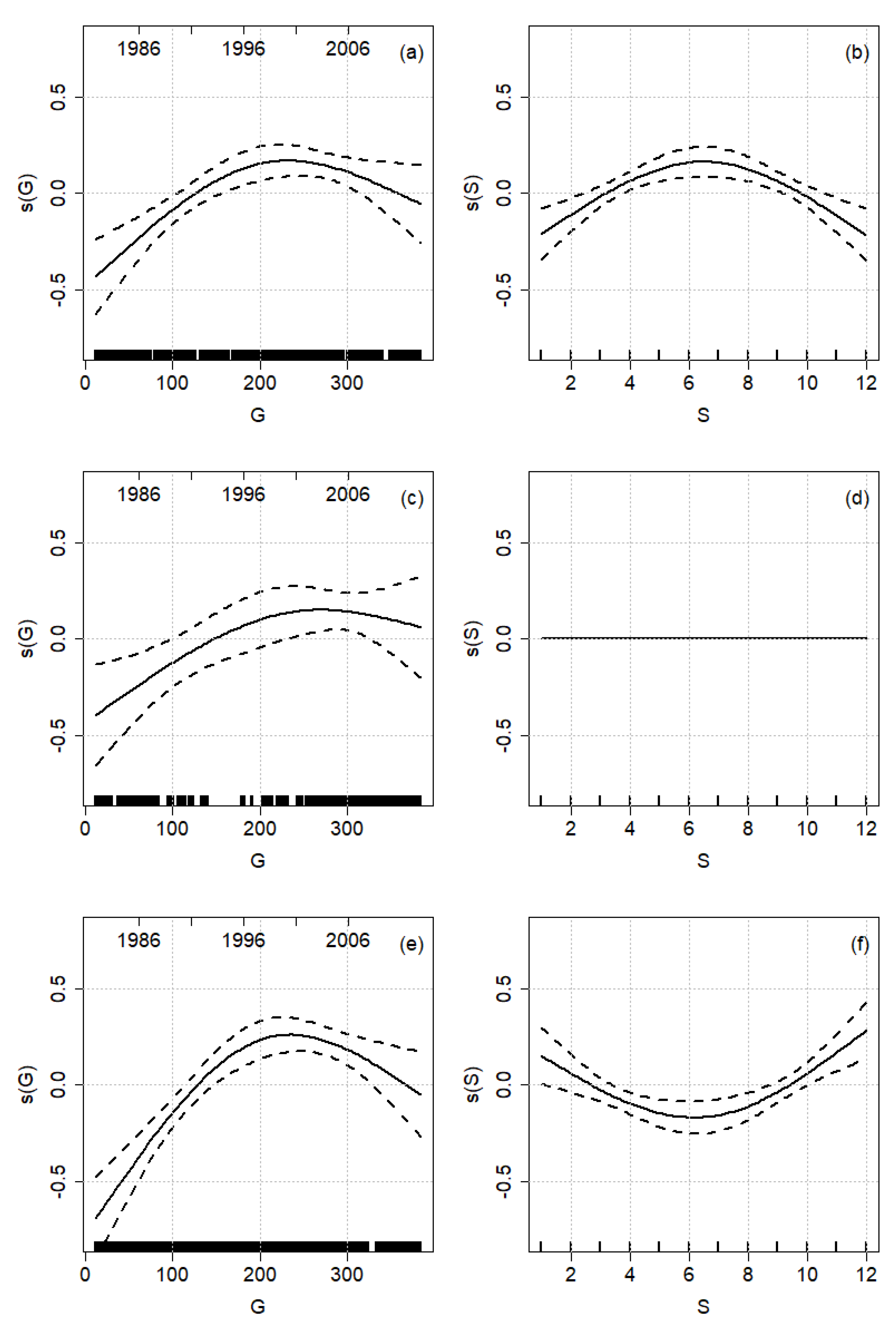
GAMM also allows inspecting the trends in the individual variables. The panels in Figure 6 represent the impact of the G and S variables in model S1. The x-axis represents the values of the variables while the y-axis represents the marginal change in the predictand relative to the mean value (in this case ) as a result of the impact of the variable (and the effect of all other variables removed). For example, for C1 and , early in the analyzed period, streamflow is higher than the average (negative values on the y-axis), but streamflow decreases over time (gets less negative on the y-axis) over time. Later in the period (after about 150 months), the streamflow is lower than the average (positive values on the y-axis), but this effect reduces again towards the end of the period when the variable dips back to a negative response. This indicates a return to higher than average streamflow towards the end of the overall period. This response is similar across the three catchment scales (Figure 6c,e).
The linear response in model L1 is less informative. Here, the slope of G is positive (Table 4), and this only suggests a long term decrease in streamflow (as there is a long term increase in the ). Interpreting the seasonal trend at C1, this is concave up, suggesting lower than average streamflow in early winter, and higher than average streamflow in the summer (Figure 6b). For C2, where the seasonal trend in model S1 is not significant (Figure 6d), the GAMM model produces a flat line around 0, as a result of the shrinkage splines used in the model [23]. For C3, the seasonal response is reversed and suggests a higher than average streamflow in the winter in this smaller headwater catchment, while lower than average streamflow occurs in summer(Figure 6f). However, since in models S1 and L1, some of the other trends can be incorporated in the seasonal and global trends, the significance of the responses needs to be retested after inclusion of other variables.
To identify if forest cover () and the growth in water licenses () can explain the trends in the residuals, these variables are now included step by step in the model. The next step in the analysis involves the models L2 and S2, which consider G, S and as explanatory variables. Model L2 and S2 have higher adjusted than models L1 and S1, indicating these models explain more of the variation in (Table 3). These models specifically test whether explains the trend better than G or S, as the shrinkage spline used [23] will allow insignificant variables to shrink to 0.
In model L2 and S2 G is no longer significant for catchments C1 and C2 while in C3 G remains significant. This suggests that for the models for C1 and C2 the smooth trend explains the trend in the data better than G, and there is no difference in whether G is considered a linear trend (L2) or is a smooth trend (S2). The seasonal variable remains significant in all models for all catchments (Table 3).
The next level of models involves L3 and S3 which include G, S and . This tests the significance of and whether this explains part or all of G or S. In this case, is highly significant for C2 (p < 0.001). Moreover, is also significant for C1 and C3 if G is considered strictly linear (model L3). This suggests that the explains the non-linear variation that in model S1 was captured in G. However, models L3 and S3 for C1 and C3, respectively, explain less of the variation in the data (adjusted ). This indicates that is lesser explaining variable compared to in model L2 and S2 (Table 3). In contrast for C2, models L3 and S3 explain more variation than models L2 and S2.
The last set of models (L4 and S4) aims to explain as a function of all variables (G, S, , and ). These models indicate a mixture of variables might explain , and this differs by catchment (Table 3). For C1, models S4 and L4 explain the highest percentage of the variation (22.2% for L4 and 21.4% for S4). The results indicate that is highly significant (p < 0.001) together with S, in model S4. However, model L4 explains more of the variation in the data and indicates that additional non-linearity in the data could be explained by , even though the significance of this variable is lower (p = 0.05). For catchment C2, model L4 explains exactly the same amount of variation as model L3, while S4 explains the largest amount of variation (13.4% for L3 and L4 and 14.9% for S4). The results of the variables for L4 and S4 suggests that is again highly significant (p < 0.001), and the effect of is very small (only significant at p < 0.1 in S4). For catchment C3, the results are quite complex, but once again models S4 and L4 explain the highest amount of the variation (26.9% for L4 and 29.5% for S4). In this case, the variable G is still highly significant, both as a linear trend and a smooth trend. This suggests there is some further global trend in the data which we cannot yet explain, for example due to a different land use change or possibly a global climate trend. For L4 is highly significant (p < 0.001) capturing non-linear effects in the data, not captured by S. However, is not significant at p = 0.1. In contrast, in model S4, which explains the highest amount of the variation in the data, is only significant at p < 0.1).
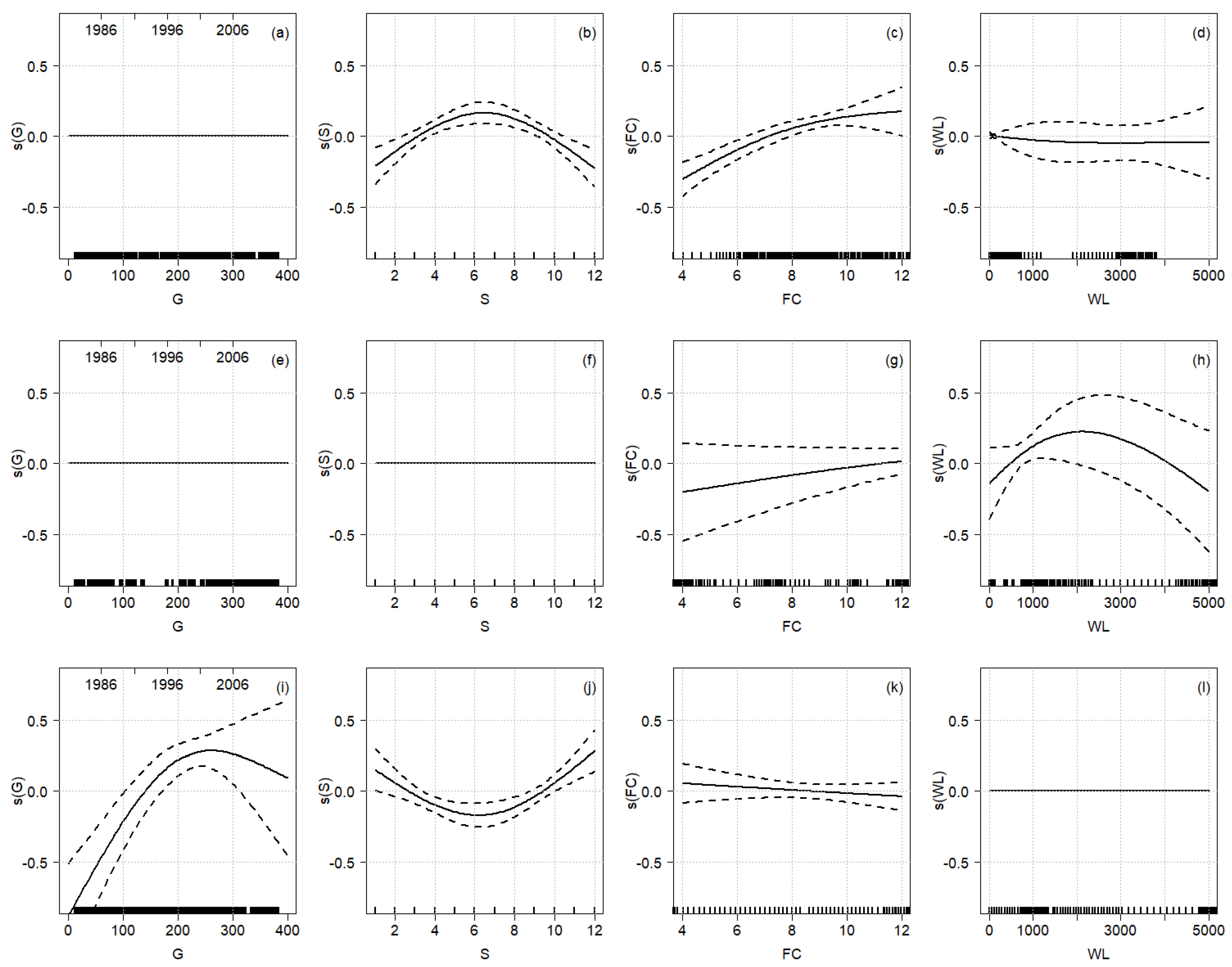
The upper panel of Figure 7a–d shows the smooth terms of the S4 model for catchment C1. As can be seen in Table 3, and are highly significant (p < 0.001). Looking at the behavior, has a smooth trend with a peak during the winter, indicating a decrease in the streamflow. Visually, appears directly proportional to in Figure 2, showing first an increase in the effect of , leading to a decrease in streamflow once is greater than 6%. Figure 7e–h highlights the smooth terms for catchment C2. Here, is highly significant (p < 0.001). The variables (p < 0.05) and (p < 0.1) also explain variation in but to a lesser degree (Table 3). The variables and visually follow a similar pattern as in C1, but the large confidence intervals around show the lack of predictive power of this variable. In contrast, peaks at a maximum value around m3/year/km2 suggests a reduction in the streamflow. For higher values of the streamflow reduction decreases, but the uncertainty increases (wider confidence intervals). This will be further discussed in the discussion. In Figure 7i–l the response curves for C3 indicate the non-significance of (Figure 7l) and the only slight significance for (indicated by the wide confidence intervals in Figure 7k). The direction of the variable might seem counter-intuitive as this suggest stream flow increases with . However, the overall curve is around 0 (no change in mean with ) and the confidence intervals overlap 0. Overall, this suggests no change in (and therefore streamflow) with in C3. The seasonal and global variables at C3 (Figure 7i,j) indicate the same trends as in the S1 model, which were discussed earlier.
4.3. Effect of Land Use Change and Water Licenses on Streamflow
In Figure 8 the effect of removing the average trends from the streamflow is demonstrated This allows visualizing the effect of the specific land use change. For C1, the effect of removing the (significant at p < 0.001) effect of , results in a substantial increase in the flow frequency curve across the full flow spectrum. The effect of was not significant in C1 and, therefore, removing this effect from the model results in almost no change in the flow frequency curve. The effect of , while significant (at p < 0.001) is only minimal in C2, as indicated in the only minor change in the flow duration curve if this variable is removed from the model. The effect of was only just significant (p < 0.1) in C2 and therefore the effect of removing this from the model is much smaller than in C1. In C3, removal of the variable suggests a decrease in the flow duration curve, but as indicated earlier, this result can probably be explained by the low certainty of the trend variable.
5. Discussion
This study demonstrates GAMM can be used to test trend hypotheses in a systematic matter based on the assumption that a rainfall-runoff model can remove variation in the data due to climate forcing. This follows the suggestions by Serinaldi et al. [25] on how to best analyse trends in data.
5.1. Seasonal and Global Trends in the Observed Runoff (Aim 1)
The significance of the seasonality variable in all the models is surprising, particularly since the trend in seasonality is not the same across the different catchment sizes (C1–C3 in Figure 7). The general assumption is that the rainfall-runoff model would remove the majority of the seasonality as it includes a measure of evapotranspiration which is strongly seasonal. However, what we are observing in the residuals is a significant seasonal trend in all the catchments. This can be explained by the fact that Santa Lucia catchment (at the Paso Pache, C1) has significant agricultural activities and this includes grain crops or other seasonal cropping routines. In contrast, catchments C2 and C3 are dominated by grassland and forest, which have typical radiation driven water requirements [36]. GR4J, as a rainfall-runoff model, does not include a “crop growth” routine, so it cannot capture the seasonal variation in evapotranspiration resulting from a growing grain crop [37]. As the land use activities differ within the catchment (Figure 1b) and physiography of the catchment varies (Figure 1a) this could result in different seasonal responses in the residuals [37].
5.2. Identifying the Effect of Exogenous Trends (Forest Cover and Water License, Aim 2)
Overall, the results suggest that in the largest catchment, the impact on the streamflow of the change in forest cover is the greatest, and it has decreased the streamflow across all parts of the flow frequency curve (Table 3 and Figure 8). In contrast, upstream in the smaller catchments, the effect is essentially unobservable (Figure 7), despite, on a percentage area basis, the forest cover being greater and the change more rapid (Figure 2a). This seems in contrast to Oudin et al. [38] who indicated that for smaller catchments the impact of land cover was greater in model performance.
The spatial arrangement of the forest cover, depending on where in the catchment the change in forest cover takes place, there could affect the flow in different ways, as is the case with nutrient losses [39]. This depends on what fraction of the actual flow is generated in the areas that are covered by forest, and how much buffering occurs within the catchment [40], and this might differ by sub catchment. For example, forest on more clayey soil in the lower catchment might impact streamflow more than forest on sandy soils in the upper catchment. There is additionally the effect of catchment size, 10% of forest cover on C1 (4896 km2) is in fact a larger total area in km2 than 20% of C3 (687 km2) and therefore this could have a large effect on the resulting streamflow. Other explanation could be differences in the hydrological response by forest type [6]. We estimated total forest cover, however in C1, the forest cover is mainly eucalyptus (grandis, dunnii, globulus), however in C2 and C3 the forest type could consist more of native forest and less eucalyptus [41].
The effect of the increased number of water licenses being provided in the catchment seems not very large (Figure 7 and Figure 8) although it is significant for the middle-sized catchment. This might be because we don’t know if users supplied with a licence actually have build water intakes, as this information is not available. In addition, the increase in provided water licenses is very recent, with a strong increase in the water licenses mainly occurring after 2010 (Figure 2b). This is particularly the case for C1. It is possible that the provided water licences have not yet fully affected the streamflow, as they might not be fully exploited. However this might happen in the future and the trends indicate that this will impact streamflow.
5.3. Further Considerations
In Figure 8, we demonstrate the mean effect of landuse change on the streamflow as a result of our GAMM analysis. In this analysis we ignore two factors. The first is the uncertainty in the GAMM analysis as indicated by the 95% confidence intervals in Figure 7. The predicted residuals are the mean response and we have not attempted to also predict the variance of the response. This means that the effect of removing the landuse variable can overestimate to actual effect. The second is based on the assumption that simulating the catchment without the landcover change (without an increase in forest cover) does not change the fit (and residuals) of the GR4J model. As a result, we can perform the analysis in Figure 8. However, it is likely that there would be a difference, as the calibration of a model would be impacted by the variance in the data and the variance in the streamflow would be impacted by the change in land cover [37].
6. Conclusions
This paper demonstrates a data-based approach that uses the combination of a rainfall-runoff model and the analysis of the residuals using GAMM to identify effects of land use change on streamflow. This methodology was demonstrated in three nested catchments related to the main water supply catchment for Montevideo (Uruguay). The analysis identified that an observed increase in forest cover significantly explained part of the variation in streamflow at the gauge draining the overall catchment. This suggested that forest cover increases were related to streamflow decreases. However, forest cover was not a significant explaining variable at the upstream gauges, despite on a % basis larger changes in cover. In addition, an increased number of water licenses appeared to have a weak effect on the streamflow at the middle gauge with no effect at the other gauges. Overall, the approach demonstrates that after removal of the “average” climate forcing effect using a rainfall-runoff model, GAMM can be used to systematically test the impact of changes in land cover on streamflow. This will also allow identifying any long term (global) or additional seasonal trends in the streamflow.
Author Contributions
For this work R.N. and R.W.V. designed and performed the experiments; R.N. analysed the data; R.N. and J.A. contribute collected data; R.N. and R.W.V. wrote the manuscript; J.A. and A.G. contribute to the review of the paper.
Funding
Instituto Nacional de Investigacion Agropecuaria, Uruguay: FPTA-341.
Acknowledgments
This paper is an output of the INIA-IRI-the University of Sydney project FPTA-341, and is funded by The National Institute of Agricultural Research of Uruguay (http://www.inia.uy/).
Conflicts of Interest
The authors declare no conflict of interest.
References
- Gleick, P.H. Global Freshwater Resources: Soft-Path Solutions for the 21st Century. Science 2003, 302, 1524–1528. [Google Scholar] [CrossRef] [PubMed] [Green Version]
- Aparicio, J.; Lafragua, J.; Lopez, A.; Mejia, R.; Aguilar, E.; Mejía, M. Water Resources Assessment: Integral Water Balance in Basins, phi-vii ed.; Number 14 in Technical Document; UNESCO Office Montevideo and Regional Bureau for Science in Latin America and the Caribbean: Montevideo, Uruguay, 2008. [Google Scholar]
- Hölzel, H.; Diekkrüger, B. Predicting the impact of linear landscape elements on surface runoff, soil erosion, and sedimentation in the Wahnbach catchment, Germany. Hydrol. Process. 2012, 26, 1642–1654. [Google Scholar] [CrossRef]
- Ren, L.; Wang, M.; Li, C.; Zhang, W. Impacts of human activity on river runoff in the northern area of China. J. Hydrol. 2002, 261, 204–217. [Google Scholar] [CrossRef]
- Gao, Z.; Zhang, L.; Zhang, X.; Cheng, L.; Potter, N.; Cowan, T.; Cai, W. Long-term streamflow trends in the middle reaches of the Yellow River Basin: Detecting drivers of change: Streamflow Trends in the Middle Reach of the Yellow River Basin. Hydrol. Process. 2016, 30, 1315–1329. [Google Scholar] [CrossRef]
- Zhang, M.; Liu, N.; Harper, R.; Li, Q.; Liu, K.; Wei, X.; Ning, D.; Hou, Y.; Liu, S. A global review on hydrological responses to forest change across multiple spatial scales: Importance of scale, climate, forest type and hydrological regime. J. Hydrol. 2017, 546, 44–59. [Google Scholar] [CrossRef]
- Yang, L.; Feng, Q.; Yin, Z.; Wen, X.; Si, J.; Li, C.; Deo, R.C. Identifying separate impacts of climate and land use/cover change on hydrological processes in upper stream of Heihe River, Northwest China. Hydrol. Process. 2017, 31, 1100–1112. [Google Scholar] [CrossRef]
- Mekonnen, D.F.; Duan, Z.; Rientjes, T.; Disse, M. Analysis of combined and isolated effects of land-use and land-cover changes and climate change on the upper Blue Nile River basin’s streamflow. Hydrol. Earth Syst. Sci. 2018, 22, 6187–6207. [Google Scholar] [CrossRef]
- Silveira, L.; Gamazo, P.; Alonso, J.; Martínez, L. Effects of afforestation on groundwater recharge and water budgets in the western region of Uruguay. Hydrol. Process. 2016, 30, 3596–3608. [Google Scholar] [CrossRef]
- Silveira, L.; Alonso, J. Runoff modifications due to the conversion of natural grasslands to forests in a large basin in Uruguay. Hydrol. Process. 2009, 23, 320–329. [Google Scholar] [CrossRef]
- Berri, G.J.; Ghietto, M.A.; García, N.O. The Influence of ENSO in the Flows of the Upper Paraná River of South America over the Past 100 Years. J. Hydrometeorol. 2002, 3, 57–65. [Google Scholar] [CrossRef]
- Camilloni, I.A.; Barros, V.R. Extreme discharge events in the Paraná River and their climate forcing. J. Hydrol. 2003, 278, 94–106. [Google Scholar] [CrossRef]
- Krepper, C.M.; García, N.O.; Jones, P.D. Interannual variability in the Uruguay river basin. Int. J. Climatol. 2003, 23, 103–115. [Google Scholar] [CrossRef]
- Kendall, M.G.; Gibbons, J.D. Rank Correlation Methods, 5th ed.; Arnold, E., Ed.; Oxford University Press: London, UK; New York, NY, USA, 1990. [Google Scholar]
- Mann, H.B. Nonparametric Tests Against Trend. Econometrica 1945, 13, 245. [Google Scholar] [CrossRef]
- Pettitt, A.N. A Non-Parametric Approach to the Change-Point Problem. J. Appl. Stat. 1979, 28, 126. [Google Scholar] [CrossRef]
- Burn, D.H.; Hag Elnur, M.A. Detection of hydrologic trends and variability. J. Hydrol. 2002, 255, 107–122. [Google Scholar] [CrossRef]
- Tramblay, Y.; El Adlouni, S.; Servat, E. Trends and variability in extreme precipitation indices over Maghreb countries. Nat. Hazards Earth Syst. Sci. 2013, 13, 3235–3248. [Google Scholar] [CrossRef] [Green Version]
- Villarini, G.; Smith, J.A.; Serinaldi, F.; Ntelekos, A.A. Analyses of seasonal and annual maximum daily discharge records for central Europe. J. Hydrol. 2011, 399, 299–312. [Google Scholar] [CrossRef]
- Zeng, S.; Xia, J.; Du, H. Separating the effects of climate change and human activities on runoff over different time scales in the Zhang River basin. Stoch. Environ. Res. Risk Assess. 2014, 28, 401–413. [Google Scholar] [CrossRef]
- Koutsoyiannis, D. Nonstationarity versus scaling in hydrology. J. Hydrol. 2006, 324, 239–254. [Google Scholar] [CrossRef] [Green Version]
- Simpson, G.L. Modelling palaeoecological time series using generalized additive models. bioRxiv 2018. [Google Scholar] [CrossRef]
- Wood, S.N. Generalized Additive Models: An Introduction with R, 2nd ed.; Chapman & Hall/CRC Texts in Statistical Science; CRC Press/Taylor & Francis Group: Boca Raton, FL, USA, 2017. [Google Scholar]
- Wang, Q.; Liu, R.; Men, C.; Guo, L.; Miao, Y. Effects of dynamic land use inputs on improvement of SWAT model performance and uncertainty analysis of outputs. J. Hydrol. 2018, 563, 874–886. [Google Scholar] [CrossRef]
- Serinaldi, F.; Kilsby, C.G.; Lombardo, F. Untenable nonstationarity: An assessment of the fitness for purpose of trend tests in hydrology. Adv. Water Resour. 2018, 111, 132–155. [Google Scholar] [CrossRef]
- Perrin, C.; Michel, C.; Andréassian, V. Improvement of a parsimonious model for streamflow simulation. J. Hydrol. 2003, 279, 275–289. [Google Scholar] [CrossRef]
- Amoussou, E.; Tramblay, Y.; Totin, H.S.; Mahé, G.; Camberlin, P. Dynamique et modélisation des crues dans le bassin du Mono à Nangbéto (Togo/Bénin). Hydrolog. Sci. J. 2014, 59, 2060–2071. [Google Scholar] [CrossRef]
- Arnaud, P.; Lavabre, J.; Fouchier, C.; Diss, S.; Javelle, P. Sensitivity of hydrological models to uncertainty in rainfall input. Hydrolog. Sci. J. 2011, 56, 397–410. [Google Scholar] [CrossRef]
- Santos, L.; Thirel, G.; Perrin, C. Continuous state-space representation of a bucket-type rainfall-runoff model: A case study with the GR4 model using state-space GR4 (version 1.0). Geosci. Model. Dev. 2018, 11, 1591–1605. [Google Scholar] [CrossRef]
- Coron, L.; Thirel, G.; Delaigue, O.; Perrin, C.; Andréassian, V. The suite of lumped GR hydrological models in an R package. Environ. Model. Softw. 2017, 94, 166–171. [Google Scholar] [CrossRef]
- R Core Team. R: A Language and Environment for Statistical Computing; R Foundation for Statistical Computing: Vienna, Austria, 2018. [Google Scholar]
- Gräler, B.; Pebesma, E.; Heuvelink, G. Spatio-Temporal Interpolation using gstat. RFID J. 2016, 8, 204–218. [Google Scholar] [CrossRef]
- Pebesma, E.J. Multivariable geostatistics in S: The gstat package. Comput. Geosci. 2004, 30, 683–691. [Google Scholar] [CrossRef]
- Andrews, F.; Croke, B.; Jakeman, A. An open software environment for hydrological model assessment and development. Environ. Model. Softw. 2011, 26, 1171–1185. [Google Scholar] [CrossRef]
- Bennett, N.D.; Croke, B.F.; Guariso, G.; Guillaume, J.H.; Hamilton, S.H.; Jakeman, A.J.; Marsili-Libelli, S.; Newham, L.T.; Norton, J.P.; Perrin, C.; et al. Characterising performance of environmental models. Environ. Model. Softw. 2013, 40, 1–20. [Google Scholar] [CrossRef]
- Bos, M.G.; Kselik, R.; Allen, R.; Molden, D. Water Requirements for Irrigation and the Environment; Springer: Dordrecht, The Netherlands, 2009. [Google Scholar] [CrossRef]
- Schilling, K.E.; Jha, M.K.; Zhang, Y.K.; Gassman, P.W.; Wolter, C.F. Impact of land use and land cover change on the water balance of a large agricultural watershed: Historical effects and future directions. Water Resour. Res. 2008, 44. [Google Scholar] [CrossRef]
- Oudin, L.; Andréassian, V.; Lerat, J.; Michel, C. Has land cover a significant impact on mean annual streamflow? An international assessment using 1508 catchments. J. Hydrol. 2008, 357, 303–316. [Google Scholar] [CrossRef]
- King, R.S.; Baker, M.E.; Whigham, D.F.; Weller, D.E.; Jordan, T.E.; Kazyak, P.F.; Hurd, M.K. Spatial considerations for linking watershed land cover to ecological indicators in streams. Ecol. Appl. 2005, 15, 137–153. [Google Scholar] [CrossRef]
- Guzha, A.; Rufino, M.; Okoth, S.; Jacobs, S.; Nóbrega, R. Impacts of land use and land cover change on surface runoff, discharge and low flows: Evidence from East Africa. J. Hydrol. Reg. Stud. 2018, 15, 49–67. [Google Scholar] [CrossRef]
- MGAP. Cartografía Forestal 2018; Dirección General Forestal: Montevideo, Uruguay, 2018. [Google Scholar]
Figure 1.
(a) Relief, monitoring system and sub-catchments of Santa Lucía at Paso Pache (C1, 4896 km), Fray Marcos (C2, 2744 km) and Paso de los Troncos (C3, 687 km). (b) Main land uses observed during 2015.
Figure 1.
(a) Relief, monitoring system and sub-catchments of Santa Lucía at Paso Pache (C1, 4896 km), Fray Marcos (C2, 2744 km) and Paso de los Troncos (C3, 687 km). (b) Main land uses observed during 2015.

Figure 2.
(a) Percentage of sub-catchment area used for forestry. (b) Water licenses.

Figure 3.
(a) Boxplot of monthly precipitation, (b) potential evapotranspiration, (c) runoff at Paso de los Troncos, and (d) mean temperature for the period 1981–2016.
Figure 3.
(a) Boxplot of monthly precipitation, (b) potential evapotranspiration, (c) runoff at Paso de los Troncos, and (d) mean temperature for the period 1981–2016.

Figure 4.
Shematic representation of the steps used to indentify the origin of trends and quantify the runoff change.
Figure 4.
Shematic representation of the steps used to indentify the origin of trends and quantify the runoff change.

Figure 5.
(a) Transformation of Relative Residuals (, gray points), linear regression of (black line) and histogram of (bars) for C1 (a,b), C2 (c,d), and C3 (e,f).
Figure 5.
(a) Transformation of Relative Residuals (, gray points), linear regression of (black line) and histogram of (bars) for C1 (a,b), C2 (c,d), and C3 (e,f).

Figure 6.
(a,c,e) Global (G) and (b,d,f) seasonal (S) terms (continuous black line) and standard error bounds (dashed line) for S1 models ().
Figure 6.
(a,c,e) Global (G) and (b,d,f) seasonal (S) terms (continuous black line) and standard error bounds (dashed line) for S1 models ().

Figure 7.
Smooth terms (continuous black lines) and standard error bounds (dashed lines) of S4 model () for C1 (a–c), C2 (e–g) and C3 (i–k) catchments.
Figure 7.
Smooth terms (continuous black lines) and standard error bounds (dashed lines) of S4 model () for C1 (a–c), C2 (e–g) and C3 (i–k) catchments.

Figure 8.
Effect of land use change and water licenses in Flow Duration Curves of Santa Lucía at Paso Pache (a), Fray Marcos (b), and Paso de los Troncos (c).
Figure 8.
Effect of land use change and water licenses in Flow Duration Curves of Santa Lucía at Paso Pache (a), Fray Marcos (b), and Paso de los Troncos (c).


Table 1.
GAMM models used.
| Model Id. | Equation (TRR Equal to) |
|---|---|
| L1 | |
| S1 | |
| L2 | |
| S2 | |
| L3 | |
| S3 | |
| L4 | |
| S4 |
Table 2.
Goodness of fit of simulated runoff at daily and monthly scale.
| Daily Scale | Monthly Scale | |||||
|---|---|---|---|---|---|---|
| Catchment | NSE | BIAS | NSE | BIAS | ||
| C1 | 0.82 | −0.04 | 0.85 | 0.91 | −0.04 | 0.91 |
| C2 | 0.81 | −0.05 | 0.84 | 0.85 | −0.03 | 0.86 |
| C3 | 0.57 | −0.07 | 0.79 | 0.78 | −0.10 | 0.80 |
Table 3.
Significance level of explanatory variables and adjusted of GAMM models.
| Catchment | Model Id. | Intercept | G | S | FC | W | Adjusted |
|---|---|---|---|---|---|---|---|
| C1 | L1 | ** | ** | *** | ⊗ | ⊗ | 0.115 |
| S1 | *** | *** | ⊗ | ⊗ | 0.188 | ||
| L2 | *** | *** | ⊗ | 0.208 | |||
| S2 | *** | *** | ⊗ | 0.211 | |||
| L3 | *** | ** | *** | ⊗ | * | 0.144 | |
| S3 | *** | *** | ⊗ | 0.188 | |||
| L4 | *** | *** | * | 0.222 | |||
| S4 | *** | *** | 0.214 | ||||
| C2 | L1 | ** | * | ⊗ | ⊗ | 0.096 | |
| S1 | * | * | * | ⊗ | ⊗ | 0.072 | |
| L2 | * | * | ⊗ | 0.125 | |||
| S2 | * | ** | ⊗ | 0.117 | |||
| L3 | . | * | ⊗ | ** | 0.134 | ||
| S3 | * | ⊗ | *** | 0.139 | |||
| L4 | . | * | ** | 0.134 | |||
| S4 | * | . | ** | 0.149 | |||
| C3 | L1 | *** | *** | *** | ⊗ | ⊗ | 0.17 |
| S1 | *** | *** | ⊗ | ⊗ | 0.285 | ||
| L2 | *** | *** | *** | *** | ⊗ | 0.269 | |
| S2 | *** | *** | . | ⊗ | 0.295 | ||
| L3 | *** | *** | *** | ⊗ | ** | 0.229 | |
| S3 | *** | *** | ⊗ | 0.285 | |||
| L4 | *** | *** | *** | *** | 0.269 | ||
| S4 | *** | *** | . | 0.295 |
Signif. codes: 0 < (***) < 0.001 < (**) < 0.01 < (*) < 0.05 < (.) < 0.1 < ( ) < 1 ⊗ variable not considered.
Table 4.
Goodness of fit of simulated runoff at monthly scale.
| Catchment | Slope (G) | p-Value |
|---|---|---|
| C1 | ||
| C2 | ||
| C3 |
© 2019 by the authors. Licensee MDPI, Basel, Switzerland. This article is an open access article distributed under the terms and conditions of the Creative Commons Attribution (CC BY) license (http://creativecommons.org/licenses/by/4.0/).
Share and Cite
MDPI and ACS Style
Navas, R.; Alonso, J.; Gorgoglione, A.; Vervoort, R.W. Identifying Climate and Human Impact Trends in Streamflow: A Case Study in Uruguay. Water 2019, 11, 1433. https://doi.org/10.3390/w11071433
AMA Style
Navas R, Alonso J, Gorgoglione A, Vervoort RW. Identifying Climate and Human Impact Trends in Streamflow: A Case Study in Uruguay. Water. 2019; 11(7):1433. https://doi.org/10.3390/w11071433
Chicago/Turabian StyleNavas, Rafael, Jimena Alonso, Angela Gorgoglione, and R. Willem Vervoort. 2019. "Identifying Climate and Human Impact Trends in Streamflow: A Case Study in Uruguay" Water 11, no. 7: 1433. https://doi.org/10.3390/w11071433
Note that from the first issue of 2016, this journal uses article numbers instead of page numbers. See further details here.