Estimating Pollutant Residence Time and NO₃ Concentrations in the Yucatan Karst Aquifer; Considerations for an Integrated Karst Aquifer Vulnerability Methodology

Abstract

Karst aquifers are a major source of drinking water with intrinsic features that increase the pollution risk from anthropogenic and natural impacts. In Yucatan, Mexico, groundwater is the sole source of drinking water, also acting as receptor of untreated wastewater due to the low regional coverage of sewer systems. To protect karst groundwater, vulnerability methodologies are widely used. Worldwide, multiple karst vulnerability schemes have been developed and tested; however, none of these consider pollutant residence time or pollutant concentration as core parameters to estimate vulnerability. This work aims to define important considerations regarding the behavior of nitrates (NO₃) in a real scenario, to be included in a new integrated vulnerability method. This work has two main objectives: to set up a groundwater model to depict as close as possible the groundwater behavior of the Yucatan karst system, and to introduce a transport model to estimate the behavior of a pollution plume. Model outcomes suggest that pollutants have a short residence time, reaching the coast in the north after 3 years. Well fields are also affected by pollution at variable NO₃ concentrations. Results can be further discretized to establish a base and to include these parameters as part of a new integrated groundwater vulnerability approach.

1. Introduction

Karst refers to a landscape where solubility of carbonate rocks allows the formation of caves, sinkholes and conduits [1]. Karsts aquifers are sensitive to pollution due to their intrinsic features including acting as a bypass between surface and water table, which allows pollutants to reach groundwater more easily and faster with little to no degradation in comparison with unconsolidated aquifers [2,3]. Besides the low natural protectiveness of karst, global change factors and urbanization increase the pollution risk in areas where wastewater and rainwater directly infiltrate into the aquifer. The Yucatan peninsula is an outstanding area for its karst features; however, the lack of systems to collect and treat wastewater enhances the pollution stress on the aquifer. Nowadays, the Yucatan aquifer is threatened from pollution sources at the surface and salt water intrusion [4]. Use of artisanal septic tanks is a common practice in Yucatan State. Since they are not impermeable, constant infiltration of wastewater into the aquifer occurs. This situation increases the pollution risk of well fields located in the periphery of urban areas [5,6,7].

Local studies have assessed both the presence and the possible vulnerability implications of NO₃ pollution in the Yucatan State (hereinafter Yucatan). Most of them conclude that some areas have already exceeded the permissible concentrations for human consumption according to national water quality standards [8,9,10,11,12,13]. The most relevant pollution scenario occurs in the sub-surface of Merida city. Due to a high population density and the lack of wastewater systems, a continuous infiltration of wastewater from artisanal (permeable) septic tanks has created a pollution plume contaminating the upper 15 m of the aquifer below the city [4,14]. However, the occurrence of this phenomenon in the subsurface of other cities in the region has not been investigated. In general, the actual anthropogenic scenario in Yucatan shows evidence of the continuous infiltration of pollutants from different sources including housing, poultry, livestock, landfills and industry.

Vulnerability maps are a first step in the development of protection strategies; these multi-parameter methodologies estimate the travel time of a theoretical immutable pollutant from the surface to the water table, based solely on the intrinsic characteristics of the area and established definitions of intrinsic vulnerability [15,16]. Nevertheless, other important processes like pollutant residence time in the aquifer and pollutant concentrations that occur in real scenarios are not considered because the inclusion and evaluation of two or more independent criteria can lead to ambiguous results in a vulnerability analysis [17].

The current pollution scenario faced by Yucatan highlights the need to evaluate groundwater vulnerability in order to support protection strategies and a sustainable approach for the development of the region. However, relying on vulnerability maps, which only estimate the theoretical travel time from the surface to the water table can lead to questionable vulnerability classes due to their lack of correlation with regional characteristics [18]. Therefore, residence time and concentration of pollutants are important parameters to be analyzed and included as factors to estimate vulnerability classes for present and future scenarios. This could help to more accurately determine well protection areas or allocation, hazards management and future urban areas according regional development strategies. This work presents a model aiming to analyze pollution plume behavior under the city of Merida and its possible repercussions on well fields and communities located in the periphery. Analysis of NO₃ concentrations and the travel time of pollutants will serve as a basis to propose important considerations to be taken into account in an Integrated Karst Aquifer Vulnerability methodology (IKAV).

2. Materials and Methods

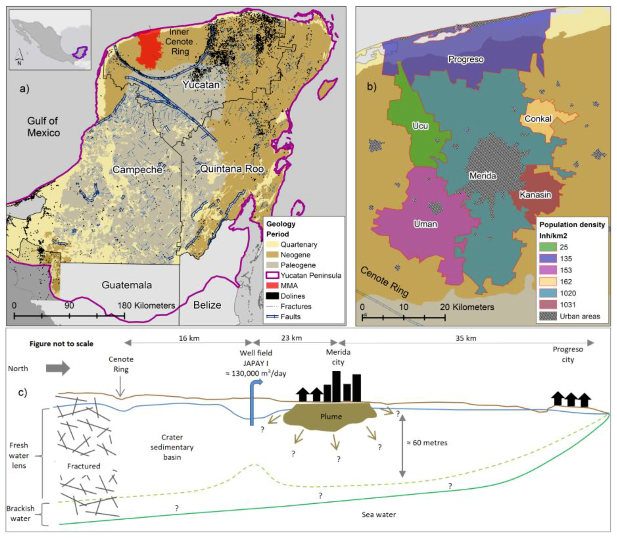
2.1. Study Area

The Yucatan Peninsula is located in the southeast of Mexico and is one of the biggest trans-boundary aquifers in the world—around 165,000 km². It is shared by Mexico, Guatemala and Belize [19]. The Mexican part includes the states of Yucatan, Campeche and Quintana Roo (Figure 1a). The Peninsula is composed mainly of limestone, with dolomite and anhydrite from the Mesozoic and Cenozoic periods reaching thicknesses > 1500 m [20]. The Peninsula aquifer contains a well-developed conduit system at variable scale ranges with primary and secondary porosity in the rock matrix [19]. Around 7.5 Mm³ of groundwater per year is extracted for human consumption [21]; however, fresh water extraction does not jeopardize the water availability since aquifer recovery is constant and fast [22]. Water balance in the region is positive, with a high availability per capita of about 7600 m³/person/year [23]; this value is high compared to the Mexican national average.

Yucatan is a developing area, which places groundwater resources under special pollution stress and therefore, calls for strong protection policies. Yucatan is characterized by a tropical weather with a marked precipitation regime with variations in time and space. Mean precipitation ranges between 200–400 mm/year along the coastal area and 1000–1200 mm/year in the southeast [24]. Two distinctive periods are characterized: dry, from November to April, and wet, from May to October. The present study focuses on Yucatan, specifically on the Merida Metropolitan Area (MMA). With around 1.1 million inhabitants, out of the total Yucatan population of 2.1 million, the MMA is a densely populated area composed of six municipalities where urbanization is continuously increasing (Figure 1b). The MMA is located inside the hydrogeological region known as the Inner Cenote Ring (ICR), one of four hydrogeological regions in Yucatan [25]. The ICR, also known as the Chixchulub sedimentary basin, is delimited by a semi-circular belt of approximately 180 km in diameter [26]; this belt, also named the Cenote Ring, has a high sinkhole density. This ring is considered to be a surface expression of an asteroid impact at the end of the cretaceous period [27]. The ICR is a relatively new sedimentary basin with a low level of karstification, although it is fractured, which explains the low number of sinkholes inside the ring compared with the crater rim. Some of the main characteristics of the area are the flatness of the terrain and lack of surface flow. The ICR has a mean slope of 1.5% and an average altitude of 28 m above sea level, except for a small area in the southeast of the inner ring. The flat topography and fracturing do not allow generation of surface streams, infiltrating precipitation at fast rates [28]. Additionally, flatness and high hydraulic conductivity originate in low hydraulic gradients ranging from 7 to 10 mm/km with groundwater flow in a north-west direction [29].

The Yucatan aquifer faces constant pollution since sanitary sewer systems are almost non-existent [4]. Only around 10% of the generated grey and black water is treated in Yucatan. Groundwater pollution risk increases in the MMA due to the increasing population density and the disposal of household and industrial wastewater, which is mainly disposed into artisanal septic tanks. Wastewater undergoes short residence times, a couple of hours, in such tanks because they are not sealed; therefore, untreated wastewater percolates and reaches groundwater almost immediately [14,30]. This continuous infiltration from permeable septic tanks has created a plume, contaminating the upper 15 m of the aquifer below Merida city [31]. However, in recent years the extension of this pollution plume has been measured, reaching up 20 m of depth (L. Marín, personal communication, July 2016) but its extension and hydraulic behavior is still unknown (Figure 1c). Additionally, in urban areas, rainwater infiltrates directly into groundwater through boreholes located along the streets; this is a common practice for rainwater disposal in this region. Conceptualization of the general Yucatan aquifer shows an unconfined fresh water lens floating above saline water which intrudes more than 40 km inland [32,33]; the exception is an area along the coast that is classified as an aquitard [34]. For simplification purposes, this aquitard is not included in the model presented in this work.

2.2. Methodology

2.2.1. Modeling Approach and Conceptual Model

To estimate pollutant residence time, groundwater modeling was carried out using MODFLOW code 2005 run in Model Muse version 3.10.0.0 (released in March 2018). The working space was built by dividing the MMA into 50 columns and 70 rows with square grids of 1 km². For output analysis purposes, an additional discretization was made between columns 21 to 58 and rows 30 to 70 with a grid size of 0.0025 km² (Figure 2). Model discretization was performed by importing a Digital Elevation Model (DEM) into an ASCII file using ArcGIS version 10.5. To get model top elevation and to define the thickness of sub-surface layers, the fitted surface interpolation included in MODFLOW was utilized. The bottom of the aquifer was defined at 80 m below the surface. Studies have estimated the saline interface as around 58 m of depth below Merida city. Since the area of interest in this work is the MMA, this depth is representative enough. Hydraulic conductivities (K) are the same as those estimated from a groundwater flow model in the area assuming EPM behavior presented in the work of González [22].

To describe turbulent flow in the karstic aquifer, the Conduit Flow Process (CFP) package is used [35,36]. However, the CFP package has a drawback when modeling target pollution studies due to its incompatibility with the groundwater solute transport simulator of MODFLOW (MT3DMS). Therefore, two modeling steps were applied to solve this problem:

• The CFP was applied for particle tracking to obtain a general idea of the residence time of any particle in the aquifer, not considering transport processes.
• An equivalent porous media (EPM) model was adjusted with the CFP parameters to enable the MT3DMS to run with nitrate data to analyze the pollution plume behavior within the study area.

The void diameter percentage, required for the CFP, was set at 0.9 given the existence of preferential flows paths at different depths of the aquifer. However, as a pre-test, the void value was evaluated between 0.9 and 0.5, without significant effects. Reynolds’s numbers were maintained at 2000 and 4000 as the default settings in the program.

2.2.2. Assumptions

Since the study area is part of a major trans-boundary coastal aquifer, some simplifications to define the system were taken for the numerical model; these are as follows:

• Temperature and density remain constant through the whole system, which implies that the saline interface does not play an important role even though it is a coastal aquifer.
• The saline intrusion occurring inland, 110 km from the coast towards the Cenote Ring, does not have a great impact in the fresh water lens behavior. Therefore, the saline interactions were not taken into consideration. This is supported by reports and studies performed by water authorities in the area [37,38,39,40,41]. Currently, there is no model derived from CFP flow solutions that can be coupled with the sea water intrusion process [42]. Since the CFP has at least two different ways to solve the conduit problems, it was decided to use the simplest one: layers of turbulent flow imbedded with laminar flow zones. This decision is based on previous studies which suggest at least three different preferential flow paths located between 11 to 12 m, 15 to 16 m, and 29 to 32 m of depth [43].
• The aquifer was simulated using an EPM approach for transport since the study area is located inside a young sedimentary basin with low development of karstic features such sinkholes and caves; also, the fracture density is quite low in comparison with areas outside the ICR.
• Steady state was assumed given the low variability in the water table time series. This also means that the current status of the aquifer is labeled as underexploited.
• Recharge was assumed to be instantaneous, thus no process occurring within the vadose zone was included. In order to model what happens in the unsaturated zone, information regarding depth, conductance and some other parameters, which are not available for the region, are necessary to run the unsaturated zone flow (UZF) package in Model Muse. This is a major simplification that neglects the possible simulation of the Epikarst part of the aquifer and its buffer role in pollutant adsorption.

Available public data was gathered and managed to create the necessary input files for the model (

Table 1. Available public data bases used to build the Yucatan model.

Data Source	Type of Database	Data Treatment
INEGI: Database #1 (public)	Edaphology shape files; hydrogeological division; Lithology shape files.	Selected to compute Recharge rates using APLIS methodology.
CONAGUA: Database #2 (digital)	Monitors network time series and reports; precipitation time series (from 1995 to 2015).	Used to build transport model assuming diffuse infiltration in the Merida Infiltration basin object.
JAPAY: Databases #3 (digital)	Waste water volumes and quality.	Used to build transport model assuming diffuse infiltration in the Merida infiltration basin object.
USGS	Digital elevation model, Aster GDEM 30 m resolution.	Base for layers thickness and groundwater levels.

). Recharge was computed using the multi-parameter GIS-based methodology APLIS, (altitude, slope, lithology, infiltration and soils respectively) to take into consideration in situ characteristics of karst areas [44].

2.2.3. Packages

The MODFLOW packages used for CFP and EPM simulations are described as follows:

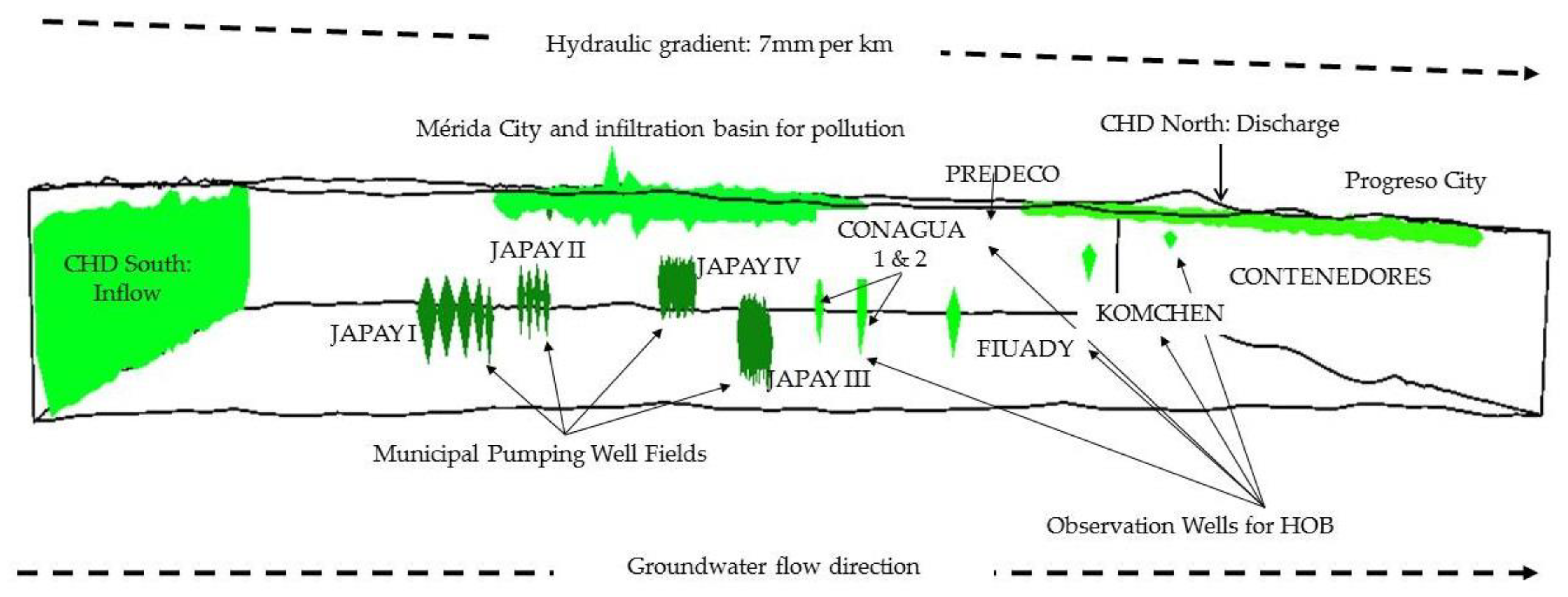
• Time-Variant Specified-Head Package (CHD): for the north boundary of the study area, a constant head of 0 m (sea level at the coastline) was established. The discharge area towards the ocean has variable thickness along the coast with depths ranging between 5 and 18 m [19,45]. The CHD was also established at the south limit towards the cenote ring. Hydraulic heads in this boundary were computed interpolating point measurements provided by the water authority (CONAGUA) time series from 2002 to 2015 with recordings, on average, every 4 months.
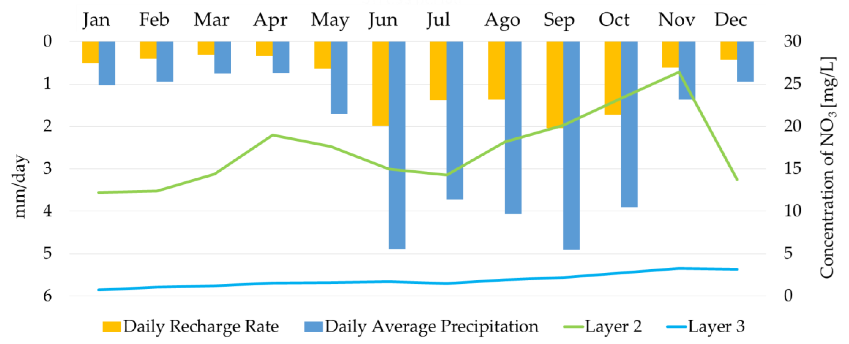
• Recharge (RCH): Since the aquifer recovers in the range of hours, according to local studies and time series of water table levels, the storage does not change on average for a hydrological year. Monthly recharge rates were estimated to run the model with 12 stress periods; each period of 8,4600 s, or one day, represented each month in a steady state condition. For the transport model, a whole stress period of 60 years was run in transient mode using a computed average recharge out of the 12 individual stress periods; recharge was further discretized according the APLIS methodology values (Figure 3).
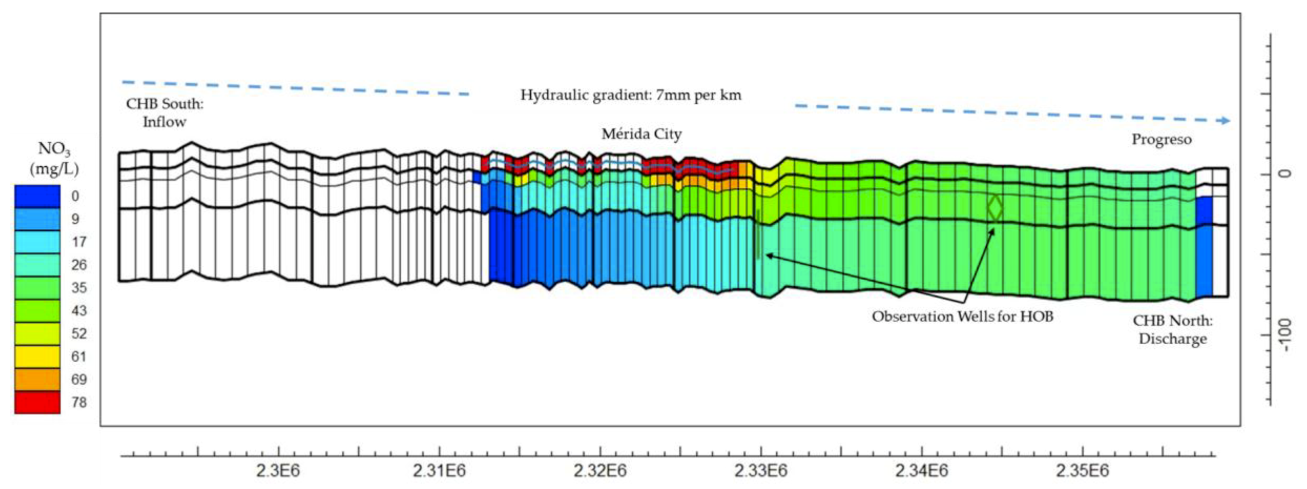
• Head-Observation (HOB): This package was used to define real observed head values. These values were used to calibrate the model. MODFLOW compares observed values with calculated ones from the program solutions and give useful statistics to calibrate the model once it has been solved. In the model, each HOB element (an observation well) is defined within a grid, assigning a head value from available time series of head observations. Then, the model computes the residuals between modeled and observed heads, giving in return a RMSE value that helps to define how accurate the model is.

For analysis purposes two places were defined as the origin of the particles: the constant head at the south of the MMA and Merida city. The former was selected to investigate the time it would take for particles to reach the coast to assess the effects of the pumping well fields distributed in the Merida city periphery and to evaluate if a preferential flow path (layer 3) exerts influence on particle movement. The later was defined to evaluate the pollution plume behavior in the Merida sub-surface.

Default values for transport were used and the activated packages for MT3MS were the basic transport (BTN), the advective-transport (ADV), dispersion (DSP), sink and source mixing (SSM) and the generalized conjugate gradient solver (GCG) pane. The species particle was NO₃ and the finite differences solver was used, code 0. At the beginning of the transport simulation, plumes are constrained near to the areas where the pollutant infiltration takes place. Simulations in this work do not consider the probable increment of NO₃ due to economic and population growth. A 3D representation of the model is displayed in Figure 4.

2.2.4. Calibration

To calibrate the model, two parameters were adjusted along the process: hydraulic conductivity for the X and Z axis (first K_x and then K_z, if the vertical infiltration is higher) and recharge rates. The time series for monitoring wells from 2002–2015, provided digitally by CONAGUA, served to analyze the values adjusted during the calibration process.

After several trials it was evident that the modifications in the K_z were not significant. Therefore, the only parameter left for trial was K_x. It was decided not to go above the suggested values of K_x found in the literature since they are already quite high even for karst standards according to Marín [29]. Calibration was ended at the best RMS value (0.2221) without going beyond the suggested K_x values of 1.115 m/s. There are no uniform criteria to define what constitutes a good RMSE, so we defined a threshold of 0.2500 to stop the calibration.

Table 2. Parameters obtained after calibration to run the transport model.

Parameter	Value	Comments
Recharge rate	Coastal area = 2.5 times the precipitation raster input file Metropolitan area (not including Merida City) = 0.2 times the precipitation raster input file Rest of the area = 0.0025 times the precipitation raster input file	Most of the coastal area has high hydraulic conductivities since sandy textures cover part of the area. Despite a layer, acting as a semi-unconfined aquifer and existing near the coastline, it was not considered in this work. This adjustment was performed since that recharge rates were both underestimated and overestimated with the GIS methodology APLIS
Hydraulic Conductivity (Kx)	Layer 1 = 1 m/s Layer 2 = 0.5 m/s Layer 3 = 1.115 m/s Layer 4 = 1 m/s	A better RMSE was showed with Kx for layer 1 and 2 with inversed values. Nevertheless, we consider that this configuration did not depict the initial assumptions about layer 1, behaving as Epikarst.

displays best fit for CFP parameters achieved by manual calibration. Values for K_z were all fixed as 1.115 m/s.

Recharge plays a fundamental role in the water budget of the study area with at least 30% of the contribution to the final discharge. Although the main input is the groundwater flow coming from the south, recharge is expected to be a driven hydraulic process when it comes to pollutant behavior. Recharge values, officially reported by the water authority, are part of a study of the whole aquifer. The average recharge for the MMA is approximately 0.18 Mm³/km² according to the study mentioned above; the recharge rate obtained after calibration is approximately 0.23 Mm³/km², which indicates that the model tends to overestimate recharge. However, modeled discharge values are close with those reported by CONAGUA [21]. Appendix A

Table A1. Initial parameters used to run de model before calibration.

Parameter or Package	Values
Layers: Layer 1 to 3 are convertible while 4 is confined.	Layer 1: DEM − 10 m Layer 2: (DEM − 35) × 0.3 Layer 3: DEM − 35 m This layer is then discretized to depict the beginning of the saturated area and the preferential flow path that tries to account for the most relevant karst feature. Layer 4: DEM − 80 m The 80 m depth for the aquifer would only account for the freshwater lens. This work only focuses on the upper part of the aquifer, regardless the saline lens in the model.
Hydraulic conductivity per layer: Given that the CFP implies one layer of preferential flow, it was defined layer 3 as the most conductive layer. Conductivity values are suggested by González in a previous numerical model where the best calibration was obtained for K = 1.115 m/s. This value t was assigned to the preferential layer.	Layer 1: 0.1 m/s Layer 2: 0.1 m/s Layer 3: 1.115 m/s Layer 4: 0.1 m/s
Boundary conditions: Constant head at sea level in 0 m. In further steps, and to adjust the conceptual model after feedback, some trials were run with GHB package (a general boundary package, which also depends on conductance). Constant head at the south of the model.	Constant head at sea level: 0 m. The discharge area was defined based on some studies that suggest that this area is quite variable and can go between 5 to 18 m thick. So, in the model, the formula was defined as: Discharge area = (Model Top − 18)/2, trying to account for the small differences in the discharge area, and made them depended on the elevation of the terrain in the model top layer. This is an arbitrary boundary that does not match with any specific karstic, topographic or political boundary, at least in the MMA model. But, when running just particles for ICR, the boundary condition is the Cenote Ring itself. This boundary condition acts as natural drainage that redirects water from inland to the ocean. It concentrates part of the discharge of the whole aquifer in the outlets of the Cenote ring.

displays the general settings utilized for the model before calibration.

3. Results

3.1. Particle Tracking

The first particle tracking simulation, with a particle release originating at the south boundary, revealed negligible effects caused by the well fields surrounding Merida with the current pumping rates. The exception is the well field JAPAY IV located in the west, suggesting the influence of a cone of depression that delays particles in this area and taking more time to move northward. The second simulation, which changed the origin of the particles to Merida city, indicated a period of 4 years for any particle to reach the coastal area in the north, particularly, in Progreso city. The main outcome for the particle tracking was the pathway itself. Given the hydraulic gradient and the preferential flow paths, particles follow a distinctive path from the north of Merida city towards Progreso. As displayed in Figure 5, particles reach two observation wells in approximately one year (FIUADY and Komchen), located approximately 15 km away from the Merida city center. The observation well PREDECO is reached after 2 years, and thus, the particles have already left the Merida city area. Particles reach the CONTENEDORES observation well, located 26 km away from the particle release point, and the southern limits of Progreso city in the third year. Outcomes also showed that there may be some concerns regarding the well field, JAPAY III.

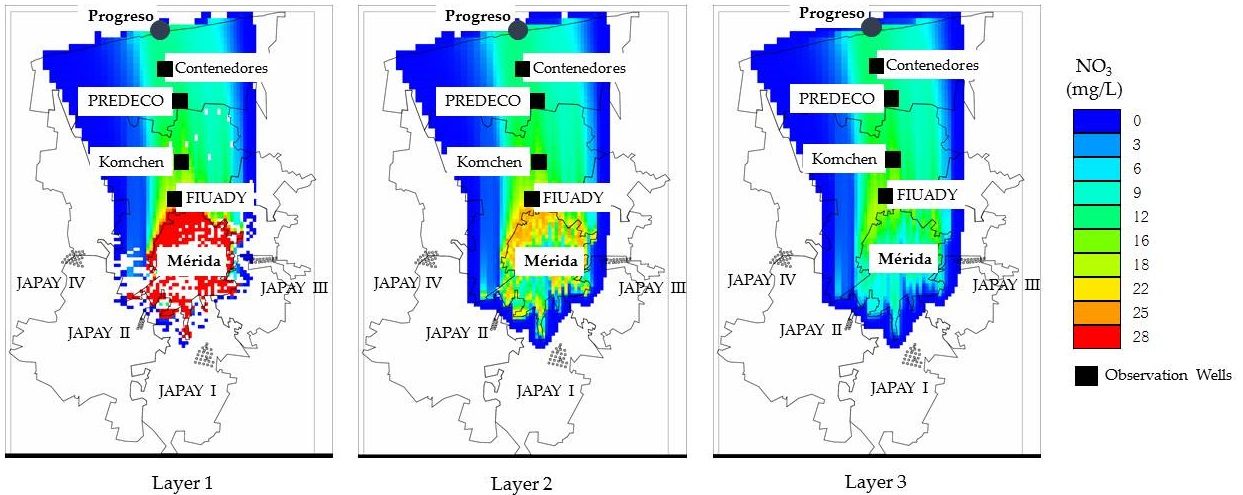
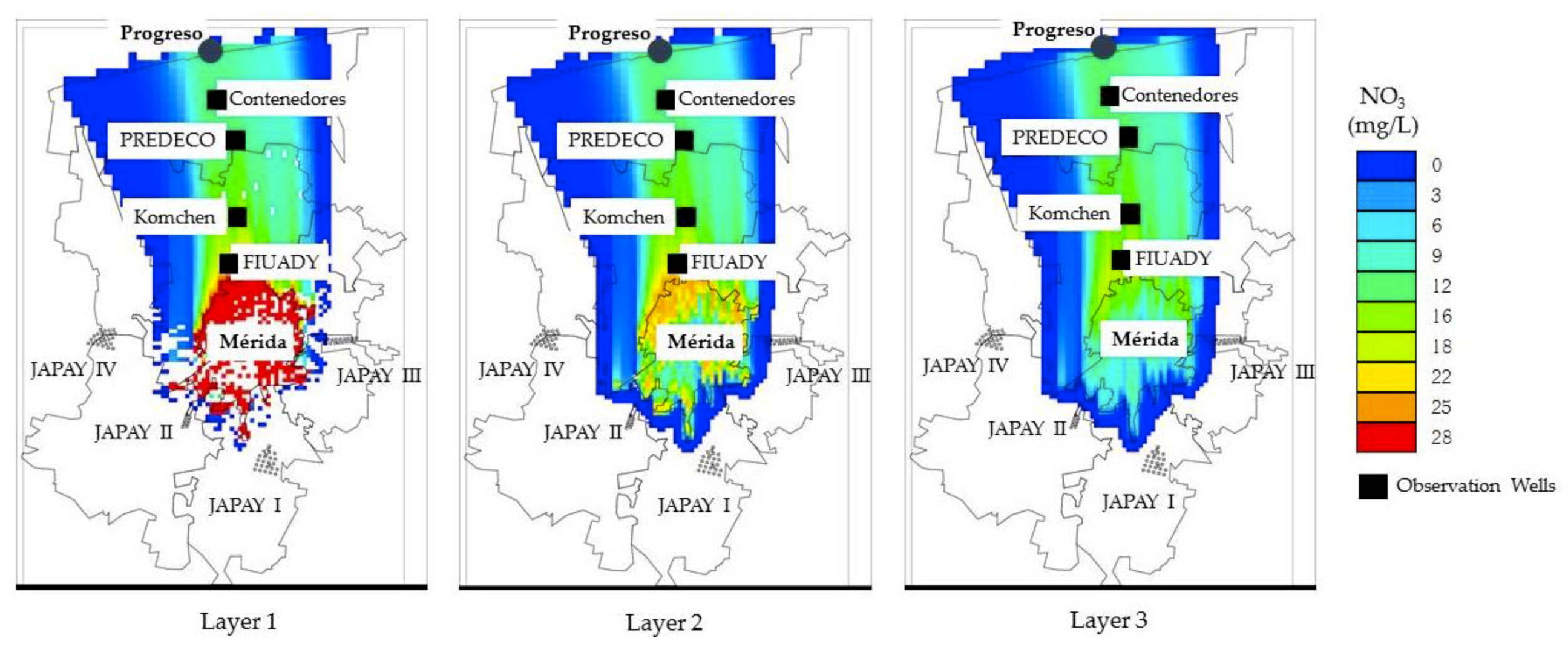
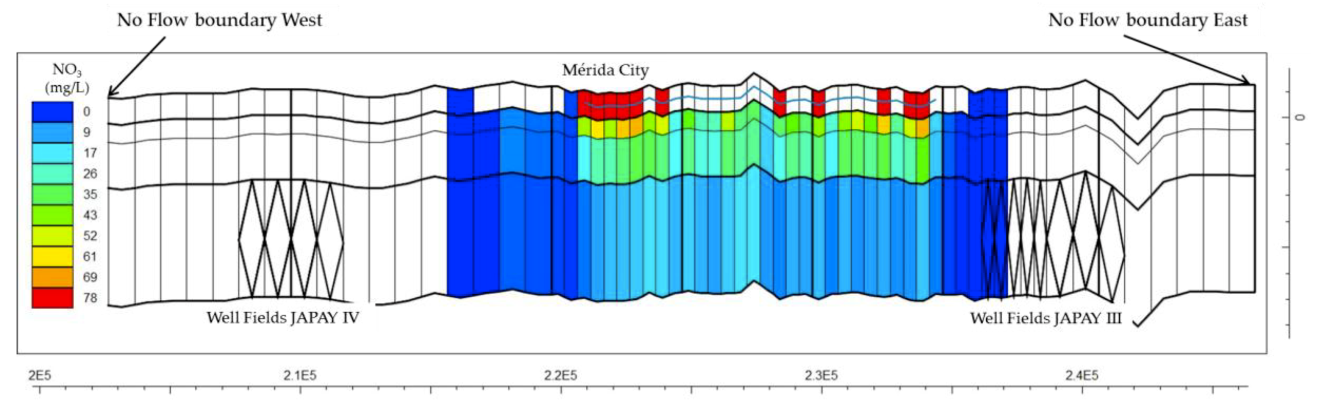
3.2. Transport Model

By the end of the simulation, the pollution plume coming from Merida city has reached Progreso City and one of the pumping well fields that supply drinking water to Merida city (JAPAY III). Even JAPAY II is slightly affected but given that cells with NO₃ concentrations lower than 0.5 mg/L were not included in the colored grid, the plume is not visible. Concentrations even reach JAPAY IV even though NO₃ concentrations are minimal. According to the model, the pollution plume also travels downward reaching the bottom of the simulated aquifer; this may affect the areas where drinking water is extracted. However, concentration curves do not show a significant increase of NO₃ in the well fields. Higher concentrations are displayed in the upper layers (1 to 3), although most dispersion seems to be located at layer 3 (Figure 6).

High NO₃ concentrations are in layer 1 where the pollution sources are located (3 m below the top of the model, simulating septic tanks); the water table does not always reach that level in the model. Therefore, MT3DMS does not show any transport results and the analysis focus on layers 2 and 3. Figure 7 also shows that pollution, even in smaller concentrations (a little above 0.001 mg/L) reaches the aquifer and the well field JAPAY III. Nevertheless, this concentration is dependent on the initial concentration established in MT3DMS to run the model with no consideration of the population growth rate or further characterization of spatial concentrations.

Pollutants move horizontally through the system, mainly through layers 2 and 3, northward. However, it seems that preferential flow paths do not exert significant effects on the movement of the pollution plume. Higher concentrations were expected along the horizontal layers, mainly in the third layer given the high hydraulic conductivity. Nevertheless, the velocity at which water travels from south to north, and the dispersion process through layer 2 influence the pollution behavior since NO₃ concentration is higher in the horizontal than in the vertical direction (Figure 8).

Concentration curves (Figure 9) show a lapse of around 300 days for NO₃ released in Merida to reach the monitoring wells at detectable concentrations. Given the general groundwater path, it seems that these wells may never reflect high NO₃ concentrations, unless the concentration released in the city increases significantly.

Recharge greatly influences NO₃ concentration patterns along the layers according to the model. Analyzing seasonal patterns, NO₃ concentration increases with recharge from July to November, and also shows an upward tendency from January to April, while from November to April it decreases. This suggests a flush effect that is more visible within the wet season. Moreover, the influence of the recharge process is restricted to the top of layer 2, the interface between the water table and the unsaturated zone (Figure 10). This phenomenon backs up the hypothesis that recharge dynamics play a significant role in the pollutants’ behavior and reasserts the role of Epikarst acting as a buffer zone that delays the movement of pollutants.

4. Discussion

The behavior of the plume under Merida city displays several interesting characteristics. Pollution concentrates mainly between layer 2 and 3, while the north of the city has a higher NO₃ concentration than the south. Also, pollution follows the hydraulic gradient and travels towards the coast. This fact could be helpful to define the vulnerable zones in further studies. In order to consider pollutants’ residence time and concentration as part of an integrated karst vulnerability approach, vulnerability becomes a relative parameter since it will be dependent on two sites: a supply target (a well field or even a city) and the point where pollution originates. The spatial distribution of the pollution plume suggests that most contaminants will be carried out by the general groundwater paths, which seem to diverge from the drinking water supply fields. It is possible that JAPAY well fields, I, II and VI, which supply water to Merida city, are not affected with the current extraction rates. However, our results indicate that JAPAY III, located in the eastern part of Merida, is more likely to extract polluted water. The plume generated underneath Merida affects this well field, which can be classified as more vulnerable compared with the others. Although pollution moves towards the coast at a similar velocity, there is a distinctive, high concentration path that moves directly towards Progreso city, and this seems to be one of the major pollution paths. There are many small communities scattered between Merida and Progreso; these communities use shallow and artisanal wells for drinking water supply, meaning they are susceptible to pollutant water in the near future, assuming that NO₃ concentrations have not increased already.

The definition of vulnerability (high, moderate or low) with regard to residence time and concentration will always depend on regional characteristics. For instance, in Mexico, the drinking water standards specify a maximum NO₃ concentration of 10 mg/L for drinking water; this of course, varies according to the country. According to the model presented here, there are several parameters to consider in future approaches to vulnerability, these are shown in

Table 3. Estimated time and NO₃ concentrations to be considered for an integrated groundwater vulnerability approach.

Vulnerability Target	Estimated Time	Maximum NO3 Concentrations
Well fields: JAPAY III	60 years	On 60 years-simulation period, the maximum concentration is 0.01 mg/L from an initial concentration of 28 mg/L coming from Merida city.
Progreso City	Two years for low recorded concentration and 4 years for a concentration higher than 5 mg/L without considering local inputs a	On 60 years-simulation, the maximum concentration is 11.8 mg/L from the original pollution coming from Merida city (28 mg/L), which means around 40% of the initial pollution concentration reached the City.
Merida City	Most pollution travels towards the coast, away from the southern municipal wells where drinking water is pump out for human consumption, mainly JAPAY II and III	Maximum concentration remains the same as the input if no changes are included, like increased rates due to population growth.
Observation wells cells (HOB) along	FIUADY around 150 days Komchen around 365 days PREDECO around 730 days Contenedores around 1095 days	Layer dependent

^a This is relevant because local NO₃ inputs in Progreso city are much higher than the average used for the Merida basin, being around 78 mg/L against 28 mg/L in Merida city. No discussion in this paper of the origin of pollution in the coastal city was made.

. This could help to establish a new, integrated methodology to prioritize areas for further investigation and to define how specific karst features actually impact the local conditions.

There are some results that suggest that pollution has spread and more sampling points are needed to assess the current situation. This work does not aim to design a new rating system for a vulnerability index, but to give some general ideas as to how this might be done and which factors may be useful in the region. We suggest that the definition of high vulnerability should be based on the areas within the pollution plume paths and the wells with higher NO₃ concentrations.

As expected, recharge shows an important influence on NO₃ concentrations. Recharge variability must also be used as a differentiation vulnerability parameter, as stated in previous studies on the region [18]. Since pollutant transport is influenced by higher recharge, months with higher rates may need different and special measures. This is also true when dealing with extraordinary natural events, such as hurricanes, which imply high recharge rates in shorter time lapses.

5. Conclusions

To the best of our knowledge, no other groundwater model, including the CFP, has been applied to this region; model files were created from scratch and the model can be improved according to newly available data. Given the specifics of the CFP, the transport model does not fully depict karstic features, which can result in an inaccurate picture of the pollution plume. To overcome these issues, a model would have to be further developed and coupled with non-linear flow packages.

The disadvantages of manual calibration are that it is a very time-consuming process, and also, the possible combinations that have already been tried may not be comprehensive enough to find all the possible optimal solutions. The main limitation in this work is the incompatibility of CFP (preferential flow paths) with MT3DMS. Results from the EPM approach do not completely reflect the karst features, but by assigning high conductivity values we aimed to compensate for the lack of a transport model in CFP. However, because the ICR a sedimentary basin, it might generally resemble an EPM model. Among other limitations, conceptualization is a dynamic task for any modeling path; the conceptual model oversimplifies the dynamics in the unsaturated area by assuming immediate infiltration, and not accounting for the delaying processes (Epikarst acting as perched aquifer) that occur within the unsaturated area. Further steps to improve the model are suggested as follows:

• The first step would be to construct an evapotranspiration file (ETV) using estimation models since only evaporation data is available for the region, in order to implement the UZF package to evaluate unsaturated phenomena.
• To set up the newly developed Non-Linear Flow Package to simulate transport in karst.
• To use a GHB at the coast to simulate tide dependency changes in coastal heads.
• To evaluate how the saline intrusion interacts with the heads and pollution behavior.

In general, this work demonstrates that groundwater in a given region can also be characterized by pollutant concentration and behavior in terms of vulnerability. The findings and considerations discussed here could serve as a basis for further development of an integrated groundwater vulnerability approach based on real situations, including the potential to analyzing future scenarios.

References

1. van Beynen, P.E. Karst Management; Springer Science+Business Media: Berlin/Heidelberg, Germany, 2011. [Google Scholar]
2. Hötzl, H. Grundwasserschutz in Karstgebieten. Grundwasser 1996, 1, 5–11. [Google Scholar] [CrossRef]
3. Goldscheider, N.; Klute, M.; Sturm, S.; Hötzl, H. The PI method–a GIS-based approach to mapping groundwater vulnerability with special consideration of karst aquifers. Z. Angew. Geol. 2000, 46, 157–166. [Google Scholar]
4. Marín, L.; Steinich, B.; Pacheco, J.; Escolero, O. Hydrogeology of a contaminated sole-source karst aquifer, Mérida, Yucatán, Mexico. Geofís. Int. 2000, 39, 359–365. [Google Scholar]
5. Ávila, J.P.; Rocher, L.C.; Sansores, A.C. Delineación de la zona de protección hidrogeológica para el campo de pozos de la planta Mérida I, en la ciudad de Mérida, Yucatán, México. Ingeniería 2004, 8, 7–16. [Google Scholar]
6. Ávila, J.P.; Sansores, A.S.; Ceballos, R.P. Diagnóstico de la calidad del agua subterránea en los sistemas municipales de abastecimiento en el Estado de Yucatán, México. Ingeniería 2004, 8, 165–179. [Google Scholar]
7. Pacheco, J.; Marín, L.; Cabrera, A.; Steinich, B.; Escolero, O. Nitrate temporal and spatial patterns in 12 water-supply wells, Yucatan, Mexico. Environ. Geol. 2001, 40, 708–715. [Google Scholar] [CrossRef]
8. Pacheco, J.; Cabrera, A. Groundwater contamination by nitrates in the Yucatan Peninsula, Mexico. Hydrogeol. J. 1997, 5, 47–53. [Google Scholar] [CrossRef]
9. Pacheco, J.; Cabrera, A.; Steinich, B.; Frías, J.; Coronado, V.; Vázquez, J. Efecto de la aplicación agrícola de la excreta porcina en la calidad del agua subterránea. Ingeniería 2002, 6, 7–17. [Google Scholar]
10. Pérez, R.; Pacheco, J. Vulnerabilidad del agua subterránea a la contaminación de nitratos en el estado de Yucatán. Ingenieria 2000, 8, 33–42. [Google Scholar]
11. Gonzalez-Herrera, R.; Martinez-Santibañez, E.; Pacheco-Avila, J.; Cabrera-Sansores, A. Leaching and dilution of fertilizers in the Yucatan karstic aquifer. Environ. Earth Sci. 2014, 72, 2879–2886. [Google Scholar] [CrossRef]
12. Torres Díaz, M.C.; Basulto Solis, Y.Y.; Cortés Esquivel, J.; García Uitz, K.; Koh Sosa, Á.; Puerto Romero, F.; Pacheco Ávila, J.G. Evaluación de la vulnerabilidad y el riesgo de contaminación del agua subterránea en Yucatán. Ecosist. y Recur. Agropecu. 2014, 1, 189–203. [Google Scholar]
13. Fabro, A.Y.R.; Ávila, J.G.P.; Alberich, M.V.E.; Sansores, S.A.C.; Camargo-Valero, M.A. Spatial distribution of nitrate health risk associated with groundwater use as drinking water in Merida, Mexico. Appl. Geogr. 2015, 65, 49–57. [Google Scholar] [CrossRef]
14. Graniel, C.; Morris, L.; Carrillo-Rivera, J. Effects of urbanization on groundwater resources of Merida, Yucatan, Mexico. Environ. Geol. 1999, 37, 303–312. [Google Scholar] [CrossRef]
15. Margat, J. Vulnérabilité des nappes d’eau souterraine à la pollution. BRGM Publ. 1968, 68, 58–70. [Google Scholar]
16. Foster, S. Fundamental concepts in aquifer vulnerability, pollution risk and protection strategy. In Vulnerability of Soil and Groundwater to Pollutants; TNO Committee on Hydrological Research: The Hague, The Netherlands, 1987; Volume 38, pp. 69–86. [Google Scholar]
17. Zwahlen, F. (ed) Vulnerability and Risk Mapping for the Protection of Carbonate (karst) Aquifers; Final report (COST action 620); European Commission, Directorate-General XII Science: Brussels, Belgium, 2004; p. 297. [Google Scholar]
18. Moreno-Gómez, M.; Pacheco, J.; Liedl, R.; Stefan, C. Evaluating the applicability of European karst vulnerability assessment methods to the Yucatan karst, Mexico. Environ. Earth Sci. 2018, 77, 682. [Google Scholar] [CrossRef]
19. Bauer-Gottwein, P.; Gondwe, B.R.; Charvet, G.; Marín, L.E.; Rebolledo-Vieyra, M.; Merediz-Alonso, G. Review: The Yucatán Peninsula karst aquifer, México. Hydrogeol. J. 2011, 19, 507–524. [Google Scholar] [CrossRef]
20. Weidie, A. Geology of Yucatan Platform. In Geology and Hydrogeology of the Yucatan and Quaternary Geology of Northeastern Yucatan Peninsula; New Orleans Geological Society: New Orleans, MA, USA, 1985. [Google Scholar]
21. Subgerencia de Evaluación y Modelación Hidrogeológica. Determinación de la disponibilidad de agua en el Acuífero Península de Yucatán; Comisión Nacional del Agua: México City, Mexico, 2002; p. 23. [Google Scholar]
22. González-Herrera, R.; Sánchez-y-Pinto, I.; Gamboa-Vargas, J. Groundwater-flow modeling in the Yucatan karstic aquifer, Mexico. Hydrogeol. J. 2002, 10, 539–552. [Google Scholar] [CrossRef]
23. Villasuso, M.; Mendez, R.A. Conceptual Model of the Aquifer of the Yucatan Peninsula. In Population, Development, and Environment on the Yucatan Peninsula: from Ancient Maya to 2030; International Institute for Applied Systems Analysis: Laxenburg, 2000; pp. 120–139. [Google Scholar]
24. CAN. National Water Commission, Statistics on water in México, 2015 ed.; CAN: México City, Mexico, 2015. [Google Scholar]
25. INEGI. Estudio Hidrológico del Estado de Yucatán; Instituto Nacional de Geografía, Estadística e Informática: México City, Mexico, 2002; p. 92.
26. Hildebrand, A.R.; Pilkington, M.; Connors, M.; Ortiz-Aleman, C.; Chavez, R.E. Size and structure of the Chicxulub crater revealed by horizontal gravity gradients and cenotes. Nature 1995, 376, 415–417. [Google Scholar] [CrossRef]
27. Pope, K.O.; Ocampo, A.C.; Duller, C.E. Mexican site for K/T impact crater? Nature 1991, 351, 105. [Google Scholar] [CrossRef]
28. Lesser, I.; Weidie, A. Region 25, Yucatán Peninsula. In Hydrogeology: The Geology of North America; Geological Society of America: Boulder, CO, USA, 1988; Volume 0–2, pp. 237–242. [Google Scholar]
29. Marín, L.E. Field Investigations and Numerical Simulation of Groundwater Flow in The Karstic Aquifer of Northwestern Yucatán, México; Dissertation, Northern Illinois University: Dekalb, IL, USA, 1990. [Google Scholar]
30. Morris, B.; Lawrence, A.; Stuart, M. The Impact of Urbanization on Groundwater Quality (Project summary Report); British Geological Survey (WC/94/056) (Unpublished): Nottingham, UK, 1994; p. 55.
31. Escolero, O.; Marín, L.E.; Steinich, B.; Pacheco, J.; Cabrera, S.; Alcocer, J. Development of a protection strategy of karst limestone aquifers: the Merida Yucatan, Mexico case study. Water Resour. Manag. 2002, 16, 351–367. [Google Scholar] [CrossRef]
32. Back, W.; Lesser, J.M. Chemical constraints of groundwater management in the Yucatan Peninsula, Mexico. J. Hydrol. 1981, 51, 119–130. [Google Scholar] [CrossRef]
33. Perry, E.; Velazquez-Oliman, G.; Marin, L. The hydrogeochemistry of the karst aquifer system of the northern Yucatan Peninsula, Mexico. Int. Geol. Rev. 2002, 44, 191–221. [Google Scholar] [CrossRef]
34. Perry, E.; Swift, J.; Gamboa, J.; Reeve, A.; Sanborn, R.; Marin, L.; Villasuso, M. Geologic and environmental aspects of surface cementation, north coast, Yucatan, Mexico. Geology 1989, 17, 818–821. [Google Scholar] [CrossRef]
35. Shoemaker, W.B.; Kuniansky, E.L.; Birk, S.; Bauer, S.; Swain, E.D. Documentation of a Conduit Flow Process (CFP) for MODFLOW-2005; U.S. Geological Survey: Reston, VA, USA, 2008.
36. Reimann, T.; Hill, M.E. MODFLOW-CFP: A new conduit flow process for MODFLOW–2005. Groundwater 2009, 47, 321–325. [Google Scholar] [CrossRef]
37. Ingenieria Ambiental del sureste SCP. In Medición Piezométrica en el Acuífero Costero (Litoral Poniente) de la Península de Yucatán; CONAGUA: Yucatan, Mexico, 2002; p. 70.
38. Infraestructura Hidraulica y Servicios, S.A. de C.V. Instrumentación y Medición de la red Piezométrica de la zona costera del Estado de Yucatán. Segunda Parte; CONAGUA: Yucatan, Mexico, 2004; pp. 1–50.
39. Consultores en Agua Potable, Alcantarillado, Geohidrología; Hidráulica Costera, I.C. Implementación de red piezométrica en la zona poniente del estado de Yucatán; CONAGUA: Yucatan, Mexico, 2009; p. 69.
40. Consultores en Agua Potable, Alcantarillado, Geohidrología; Hidráulica Costera, I.C. Segunda parte de la implementación de Red Piezométrica en la zona Poniente del Estado de Yucatán; CONAGUA: Yucatan, Mexico, 2010; p. 101.
41. Consultoría Betsco, S.A.; de, C.V. Estudio de Instrumentación de la red de Monitoreo Piezométrico del acuífero de: Península de Yucatán en la zona costera del Estado de Yucatán; CONAGUA: Yucatan, Mexico, 2012; p. 31.
42. Xu, Z.; Hu, B.X. Development of a discrete-continuum VDFST-CFP numerical model for simulating seawater intrusion to a coastal karst aquifer with a conduit system. Water Resour. Res. 2017, 53, 688–711. [Google Scholar] [CrossRef]
43. Sanchez, I. Modelo numérico del flujo subterráneo de la porción acuífera N-NW del Estado de Yucatán: implicaciones hidrogeológicas. [Groundwater flow numerical model of the N-NW aquifer sector of the State of Yucatan: hydrogeological implications]. Master’s Thesis, Autonomous University of Chihuahua, Engineering School, Postgraduate Studies Division, Chihuahua, México, 1999. [Google Scholar]
44. Andreo, B.; Vías, J.; Durán, J.; Jiménez, P.; López-Geta, J.; Carrasco, F. Methodology for groundwater recharge assessment in carbonate aquifers: application to pilot sites in southern Spain. Hydrogeol. J. 2008, 16, 911–925. [Google Scholar] [CrossRef]
45. Gondwe, B.R.; Lerer, S.; Stisen, S.; Marín, L.; Rebolledo-Vieyra, M.; Merediz-Alonso, G.; Bauer-Gottwein, P. Hydrogeology of the south-eastern Yucatan Peninsula: new insights from water level measurements, geochemistry, geophysics and remote sensing. J. Hydrol. 2010, 389, 1–17. [Google Scholar] [CrossRef]
Figure 1. General characteristics of the study area; (a) extension of the Yucatan Peninsula and main karst features; (b) municipalities composing the MMA, and (c) a basic hydrogeological representation of the Merida city sub-surface (modified from Marín [4]).
Water 11 01431 g001
Figure 2. Discretization of the study area, view from South to North. The X axis represents Universal Transverse Mercator coordinates (UTM) and Y axis depth in meters.
Water 11 01431 g002
Figure 3. Locations of well fields, monitoring wells with the spatial distribution of the recharge package. Axis X and Y display UTM coordinates in meters.
Water 11 01431 g003
Figure 4. A 3D presentation of the study site, including all active objects and packages used to run the groundwater numerical solution and the transport model.
Water 11 01431 g004
Figure 5. Particle tracking with Merida city as the particle release area. Two particles per axis were released for each grid corresponding to Merida City. A clear movement northward indicates the theoretical vulnerability of small communities between Merida and Progreso.
Water 11 01431 g005
Figure 6. Pollution plume simulation after 60 years. The pollution plume follows the groundwater flow, moving towards the coast, indicating the vulnerability of towns located in the middle.
Water 11 01431 g006
Figure 7. The east-west view of the model shows that the plume has reached at least one of the well fields that supply drinking water to the city, although with low NO3 concentrations. However, well fields supplying Merida or towns located at the west part of the city can be characterized as more vulnerable to contamination.
Water 11 01431 g007
Figure 8. Behavior of the pollution plume under Merida City. The pollution travels towards the coast north of the city, increasing its concentration in layer 2 and 3.
Water 11 01431 g008
Figure 9. NO3 concentration curves for layers 1 and 2 for selected observation wells along the Merida-Progreso transect. The minimum NO3 concentration, according to the Mexican standards for water supply, is 10 mg/L (NOM-127-SSA1-1994).
Water 11 01431 g009
Figure 10. Relationship between recharge and NO3 concentration in Progreso City according the model.
Water 11 01431 g010