Comparison of Multivariate Spatial Dependence Structures of DPIL and Flowmeter Hydraulic Conductivity Data Sets at the MADE Site


1
Center for Applied Geoscience, University of Tübingen, 72074 Tübingen, Germany
2
Research Facility for Subsurface Remediation (VEGAS), University of Stuttgart, 70569 Stuttgart, Germany
3
Kansas Geological Survey, University of Kansas, Lawrence, KS 66047, USA
*
Author to whom correspondence should be addressed.
Water 2019, 11(7), 1420; https://doi.org/10.3390/w11071420
Submission received: 11 June 2019
/
Revised: 4 July 2019
/
Accepted: 5 July 2019
/
Published: 10 July 2019
(This article belongs to the Section Hydrology)
Abstract
:We analyse two datasets of hydraulic conductivity (K) from the MAcroDispersion Experiment (MADE) site, one measured by direct-push injection logging (DPIL) and the other by flowmeter profiling. The analysis is performed using copula techniques which do not rely on the assumption of multivariate Gaussianity and provide a means to characterise differing degrees of spatial dependence in different quantiles of the K distribution. This characterisation provides better insights into the similarities and differences between the two datasets. In addition to the marginal distributions and the traditional two-point geostatistical measures, copula-based bivariate rank correlation and asymmetry measures are analysed and compared. Furthermore, the parameter estimates obtained by likelihood estimation using n-point theoretical models are analysed. This analysis confirms the similarity of the spatial dependence of K between the two datasets in terms of their marginal distributions and bivariate measures, particularly in the vertical direction. We demonstrate clear indications of the existence of non-Gaussian spatial dependence structures of K at this site. We were able to improve the estimation of the K distribution by taking into account either non-Gaussianity or a censoring threshold, which are expected to lead to a more realistic description of processes that are dependent on K.
1. Introduction
The spatial arrangement of hydraulic conductivity (K) affects groundwater flow and solute transport behaviour. If the structure of K were perfectly known, then estimates of solute concentrations over time would be much improved. However, information about the structure of K is sparse, and often simplifications such as the assumption of multivariate normal dependence (“Gaussianity”) are made. Besides the traditional two-point measures, the validity of this assumption can be evaluated and quantitatively described based on higher dimensional measures.
One such measure is the multivariate copula. Copulas were introduced by Sklar [1], and have been developed in insurance and financial mathematics [2]. Copulas are able to describe the properties of real-world data without imposing an assumption of multivariate Gaussianity. Recently, they have also been used to analyze hydrological and hydrogeological problems, both in terms of spatial data [3,4,5,6,7,8] and time series [9,10,11,12,13]. The advantage of copulas is that the spatial dependence structure can be described independently of the marginal distribution for interpolation and simulation purposes. In addition, varying degrees of dependence in various quantiles can be quantified, whereas linear geostatistics relies on one kind of average degree of dependence for a given lag. In this paper, we use a copula familiy that is derived via non-monotonic, parsimoneous transformations from the multivariate normal copula that allows for efficient parameter estimation in dimensions much larger than two, which we regard as an advantage compared to the other cited approaches.
Copula-based methods provide full multivariate stochastic models in probability space, with data-driven parameter estimation. This approach has been used to characterise the structure of K in the mildly heterogeneous sand aquifer at the Borden site, Canada, providing a means to assess the influence of the spatial dependence structure of K on the solute transport [14]. Despite the mild degree of heterogeneity at the Borden site, both in terms of a symmetric marginal distribution and a mild deviation from multivariate normality, the K field simulations with non-Gaussian spatial structures in two dimensions led to distinctly different solute transport behaviour than did those with Gaussian spatial structures [14]. A slight increase in the standard deviation of the marginal distribution together with the same multivariate model of spatial dependence led to meaningfully different solute transport behaviour, also in three dimensional space. We would expect to see such discrepancies, perhaps to a greater degree, at more heterogeneous sites.
The MAcro Dispersion Experiment (MADE) site is more heterogeneous than the Borden site. Like Borden, it has been studied extensively in the hope of better characterising the arrangement of K and associated solute transport characteristics [15,16]. Flowmeter measurements collected in the late 1980’s and early 1990’s [17,18] have served as the primary source of information on the MADE site K field. Recently, a series of K measurements using direct-push injection logging (DPIL) were conducted at the site [19,20].
Bohling et al. [21] presented a revised calibration of the DPIL data accounting for the insensitivity of DPIL responses to K variations above a certain threshold. When high-K values are encountered, injection-induced pressure changes approach the lower detection limit of the pressure transducer, weakening the quality of the signal. In contrast, the flowmeter measurements are particularly subject to uncertainty in low-K zones due to the low-flow threshold of the impeller flowmeter [17]. Measurements above (“on the right side of some threshold”, DLR) or below a threshold (“on the left side of the detection limit”, DLL), or generally within an interval (“censored measurements”) are more uncertain than those that are not censored. Despite this uncertainty, they still provide useful information, namely, that they reside in an interval. How to use this information is a long-standing issue in surface and subsurface hydrology [22,23,24]. The approaches of Bárdossy [25] and Haslauer et al. [26] allow the integration of censored measurements into copula based estimation.
The previous comparisons [20,21] concluded that the flowmeter and DPIL K data display similar large-scale patterns and remarkably similar semivariograms, despite differences between the marginal distributions of the two datasets. These similarities provide compelling evidence that both datasets accurately reflect the two-point autocorrelation structure of the K field at the site. Given the differences between observed and simulated solute transport at the site [27,28], naturally the question arises if there is some aspect of the spatial arrangement of K that is missed if the analysis is constrained to the first two statistical moments and the assumption of multivariate normal spatial dependence. The goal of this paper is to analyse the spatial dependence structure of K at the MADE site without assumptions of multivariate Gaussianity. The flowmeter and DPIL K-measurements are analysed using copulas, through both empirical measures and fitted models. Additionally, the varying level of uncertainty in the data (e.g., high-K DPIL measurements are more uncertain), is incorporated into the analysis. For comparison with traditional geostatistical methods, the marginal distributions of the two datasets and bivariate summary measures of their spatial structures are presented.
There are data-sets of saturated hydraulic conductivity (K) from four sites used in this paper:
- the dataset from Borden, Canada, where Sudicky [29] measured K using permeameters, for reference;
- the dataset from North Bay, Canada, where Sudicky et al. [30] measured K using permeameters, for reference;
- the dataset from Cape Code, Masssachusetts, USA, where Hess et al. [31] measured K using permeameters and flowmeters, for reference.
After providing the necessary background (Section 2), we will compare the following measures between flowmeter and DPIL datasets: their marginal distributions (Section 3.1), their bivariate empirical spatial dependence measures in measurement and rank space (Section 3.2), and the estimated parameters of Gaussian and v-copula models fitted to the datasets in high dimensional spaces (Section 3.3), including model fits accounting for data censoring (Section 3.4). Conclusions are presented in Section 4.
2. Materials and Methods
Details of copula theory can be found in [32,33,34] and will be not be repeated here. The bivariate copula measures, which are used to describe bivariate spatial dependence in this work, are presented in Section 2.1. Theoretical spatial copula models for high-dimensional spatial dependence are introduced in Section 2.2. In Section 2.3, parameter estimation with a censoring threshold is presented.
2.1. Bivariate Measures of the Spatial Dependence Based on the Copula
The basic concept of geostatistics is that spatially close measurements are more likely to be similar than measurements separated by larger distances. This concept is reflected in the (semi-) variogram , which relates the average variance of measurements at two locations to their separation distance .
Although copulas model dependence in high dimensions, it is also possible to compute data-based summary measures, allowing for comparisons with traditional geostatistical tools such as the semivariogram and aiding in visualisation of results. Examples of such measures are the empirical bivariate copula density, the copula-based rank correlation, and the asymmetry. These measures are based on data and are used to explore and quantify certain characteristics of two-point dependence. Based on the results of these measures, the kind of dependence can be inferred and the similarity of the spatial dependence between two datasets can be quantified.
To calculate the empirical bivariate copula density, the observations , with coordinate vectors , are transformed to probability space via the margins that were estimated via non-parametric kernel density estimation using leave-one-out cross-validation and a log-normal kernel. Then the data pairs [14]:
are classified according to separation distance, given by the magnitude of the lag vector . As with semivariogram computation, a lag tolerance is introduced and data pairs with separation distances falling within the same bin (nominal lag plus or minus the tolerance) are used to represent that nominal lag. Equation (1) can be also be applied in the anisotropic case, when the spatial structure varies significantly with direction. In this case, the data pairs are grouped according to both the magnitude and direction of . Anisotropy will be discussed in more detail later.
To evaluate the information on dependence structure provided by the bivariate copula density, the following methods can be used:
2.1.1. Bivariate Copula Density
The distribution of the data-pairs and for every is the empirical bivariate copula density for lag . The plot of the bivariate copula density for a given lag has the following properties: (1) It is symmetric about because the data pair and the data pair belong to the same . (2) The bivariate copula density presents more information regarding the relationships among data pairs than does a summary measure such as the semivariogram, which is an average variance for all data pairs with a separation distance of approximately . Data pairs whose values are both small plot near the origin and data pairs whose values are both large plot near the upper right corner of the unit square. Data pairs with one small value and one large value plot near the upper left corner and the lower right corners. In the case of no dependence, the bivariate density has no structure. In the case of a strong dependence, there are areas with high density and areas with low density. In the case of a Gaussian dependence, the proportion of data pairs on the lower left will equal the proportion on the upper right. A sequence of copula density plots for different lags provides a representation of the spatial dependence structure. More details of the bivariate copula density can be found in [35].
2.1.2. Rank Correlation
The copula-based rank correlation (Equation (2)) and asymmetry (Equation (3)) are two univariate functions of lag that can be used to quantitatively summarise the empirical copula density. The copula-based rank correlation (Rank in (Equation 2)) describes spatial dependence in a fashion similar to the covariogram (). However, since it is based on , it is less influenced by extreme values. It can be calculated as [14]
where is the number of data pairs for the lag distance . Data pairs with short lags will generally have a larger Rank value. The behaviour of Rank is similar to the behaviour of a normalised covariogram. For very short separation distances, the rank correlation is unity, and it decreases until it eventually reaches zero, indicating a lack of correlation between data pairs separated by a sufficiently large distance.
2.1.3. Asymmetry
This measure shows the difference between the densities on the two sides of the line , the line from the upper left corner to the lower right corner of the bivariate density plot. Positive asymmetry indicates stronger dependence among larger quantiles than among smaller quantiles and negative asymmetry indicates the opposite. Depending on the correlation, a typical value of Asym is between −0.03 and 0.03. As a special case, Gaussian dependence has equal dependence in both high and low quantiles and is symmetric about the line . The value of Asym in this case is zero. Thus, a value of Asym that is consistently different from zero is evidence for the existence of a non-Gaussian dependence structure.
2.2. Theoretical Spatial Copulas
This section presents a summary of theoretical spatial copulas. Spatial copula models must satisfy certain conditions beyond those required in a non-spatial multivariate context. As defined by [14], these additional conditions are:
- The bivariate spatial copula depends only on the lag vector between measurement points and is independent of the location of the measurement points.
- An n-dimensional spatial copula can be built using any subset, of size n, of the observations and describes the spatial dependence among these points.
- An arbitrarily strong dependence has to be contained.
Different copula models for non-Gaussian spatial dependence have been developed, including the v-copula and the maximum Gauss copula [14], among others. In this study, we use the v-copula, which is based on a variable, X, representing a nonlinear transformation of an underlying standard normal variable, Y:
where are the two model parameters and is an n-dimensional normal random variable with mean vector and correlation matrix . When , the v-copula approximates Gaussian conditions. Analytical expressions for the distribution of the n-dimensional marginal and the density exist [4].
This paper follows the maximum likelihood (ML)-based approach described in Bárdossy and Li [4] to estimate the copula model parameters. The dataset S is separated into w small subsets , each with data points and , because of the complexity of the computation. Then the correlation matrix for each subset is calculated as
where is the correlation function, which depends only on the vector . This correlation function can be calculated by superposition one or more correlation functions as
where is the correlation function related to the theoretical variogram, is the weight of the correlation function and is the range of the correlation function. The likelihood for each subset can be calculated from the corresponding copula density with parameter vector (Equation (7))
and
The likelihood in Equation (8) is maximised by varying . This process is repeated a number of times to reduce the influence of the choice of the subset. Finally, the average value of all of the estimation results is calculated, yielding the estimated copula parameters and .
2.3. Theoretical Spatial Gaussian Copula with Censored Measurements
To take censored data into account, censoring thresholds between 0 and 100 percent are defined as input parameters. The probability space is split into to two parts for a one side censoring threshold or three parts for a two sides censoring threshold. If the threshold represents an upper limit, data values below the threshold are considered to be crisp and those above it to be censored, and vice versa if it represents a lower limit. Then a two-step maximum likelihood parameter estimation is performed.
The first step is the calculation of the cumulative distribution function using kernel density estimation method. While calculating the likelihood function, the values of probability density function for the censored data are replaced by the area of the part below the lower threshold or the area of the part above the upper threshold [26].
The second step is the copula parameter estimation. The value of the censored data is replaced by the conditional density based on the crisp data [25]. Then, the likelihood function can be written as
where is the index of the subset with only crisp data, and is the index of the subset with both crisp and censored data.
3. Results
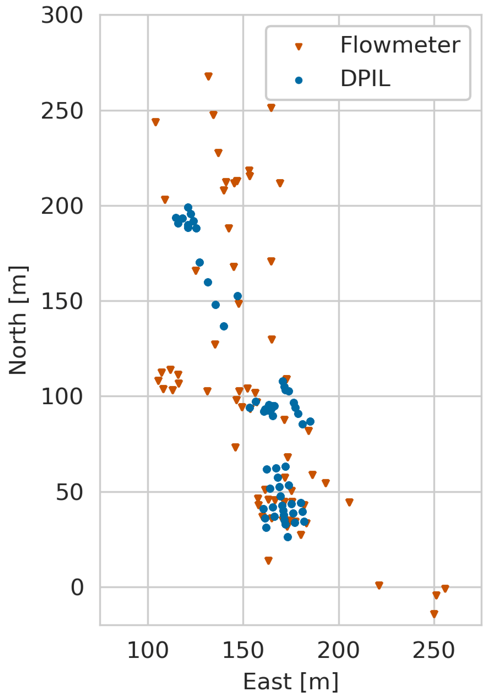
The MADE site DPIL and flowmeter measurement locations are shown on Figure 1. The vertical spacing of the DPIL measurements, 1.5 cm, is ten times finer than the typical vertical spacing of the flowmeter measurements. However, the flowmeter profiles provide better lateral coverage of the site than do the DPIL profiles (Figure 1).
In this section, the DPIL and flowmeter datasets are compared using the measures described above. The DPIL dataset analysed here is that from the revised calibration described in Bohling et al. [21]. The marginal distributions and basic statistics are compared in Section 3.1, the empirical bivariate spatial dependencies are compared in Section 3.2, and the results of parameter estimation in high dimensions are evaluated in Section 3.3.
3.1. Marginal Distribution and Basic Statistics
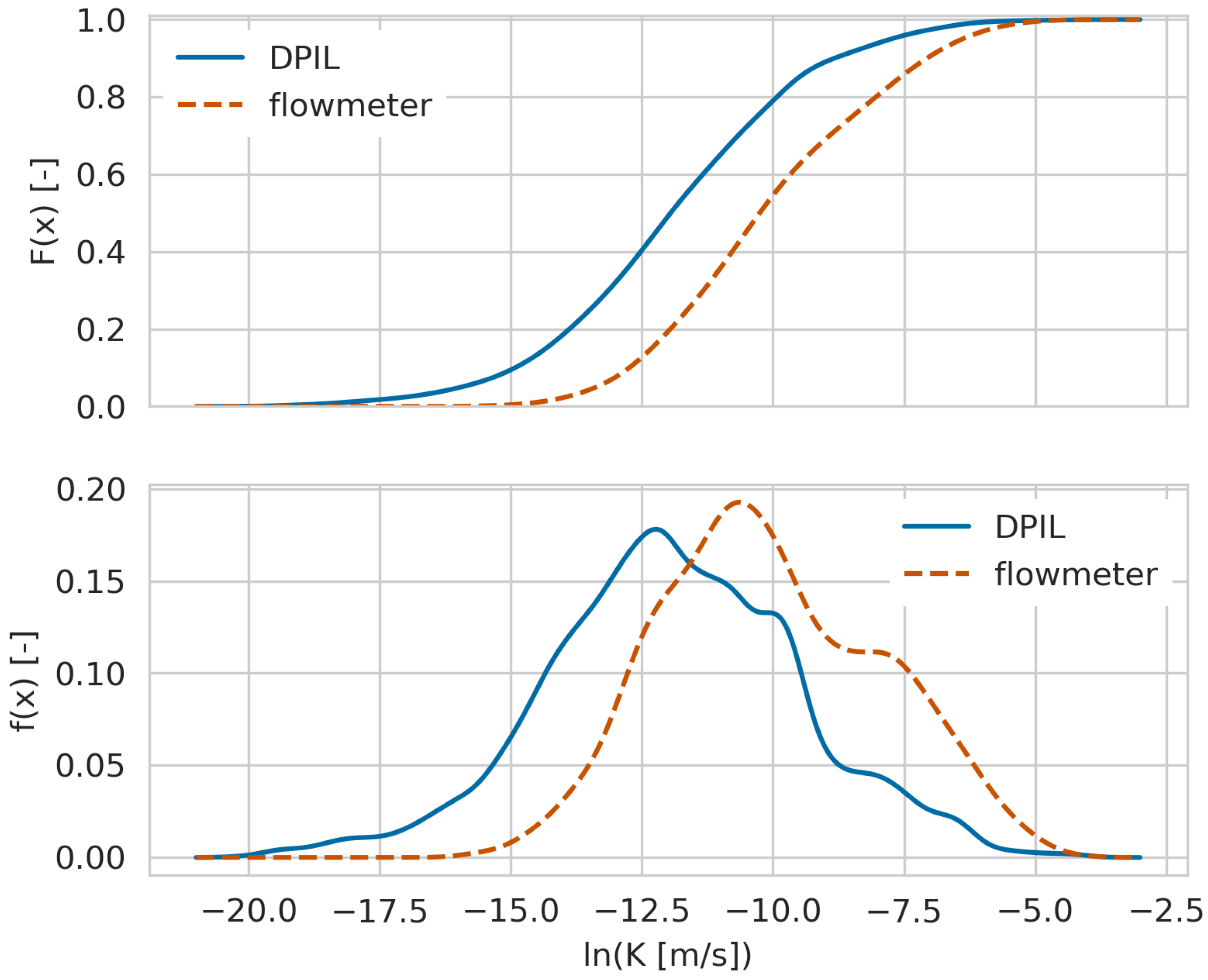
The univariate distributions of the flowmeter and DPIL logarithmic K values have similar shapes despite a shift in location. This finding is in accordance with [21]. For an improved visualisation, the cumulative density functions (CDF, Figure 2, top panel) and the probability density functions (PDF, Figure 2, bottom panel) of are plotted. The DPIL dataset has a larger portion of lower K values, a smaller portion of larger K values, and a larger spread.
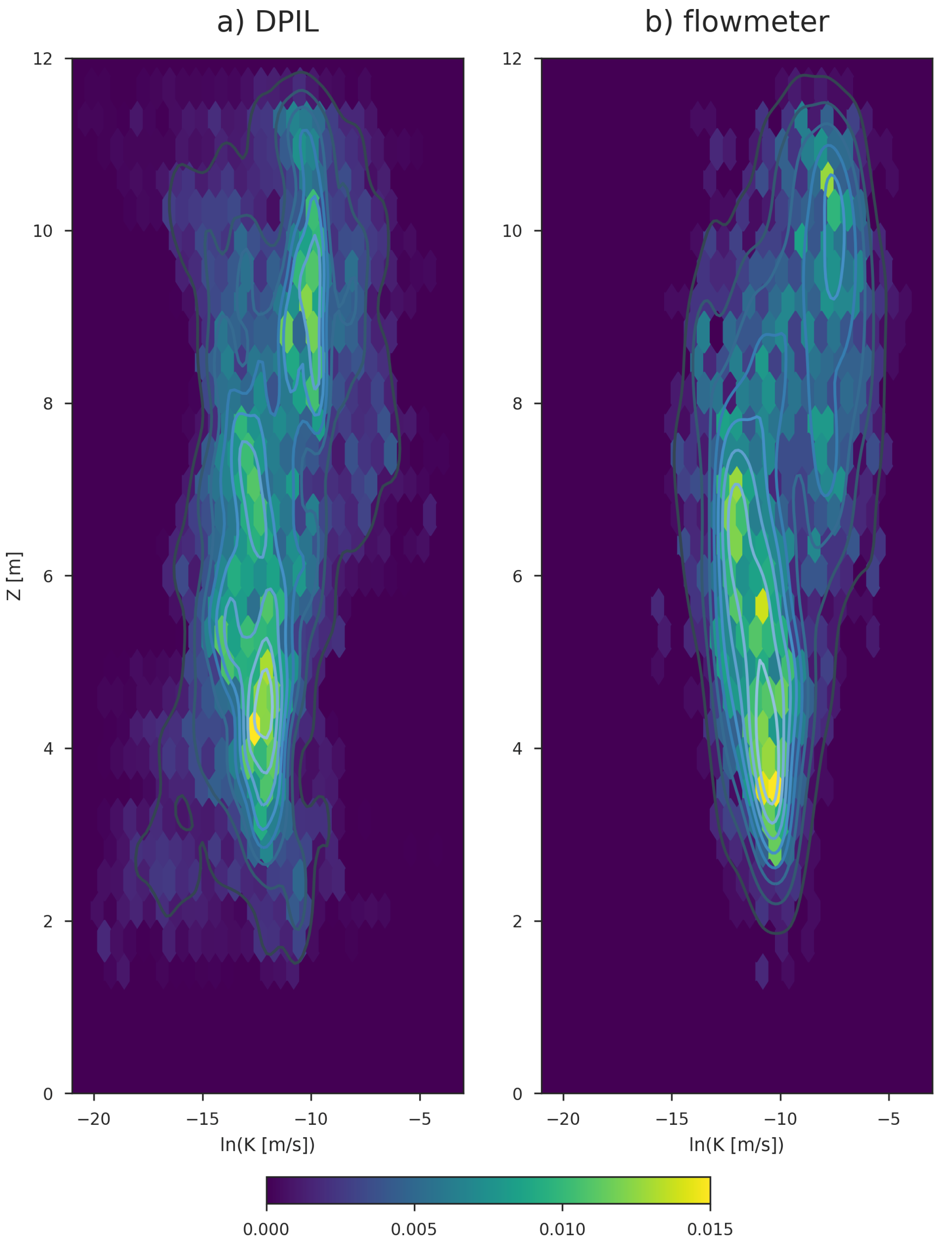
This pattern can be also seen by plotting two-dimensional histograms of versus elevation (Figure 3). Both distributions show a fairly distinct shift at about 8 m above the reference elevation (see Bohling et al. [21] for a definition of the coordinate system), with generally larger K values above this elevation and generally smaller K values below. Below 8 m elevation, the flowmeter data seem to indicate a slightly increasing trend with increasing depth, a trend which might also be reflected in the DPIL data if one considers the higher density region of the data, discounting the relatively small proportion of very low DPIL K values at elevation m.
3.2. Empirical Spatial Dependence
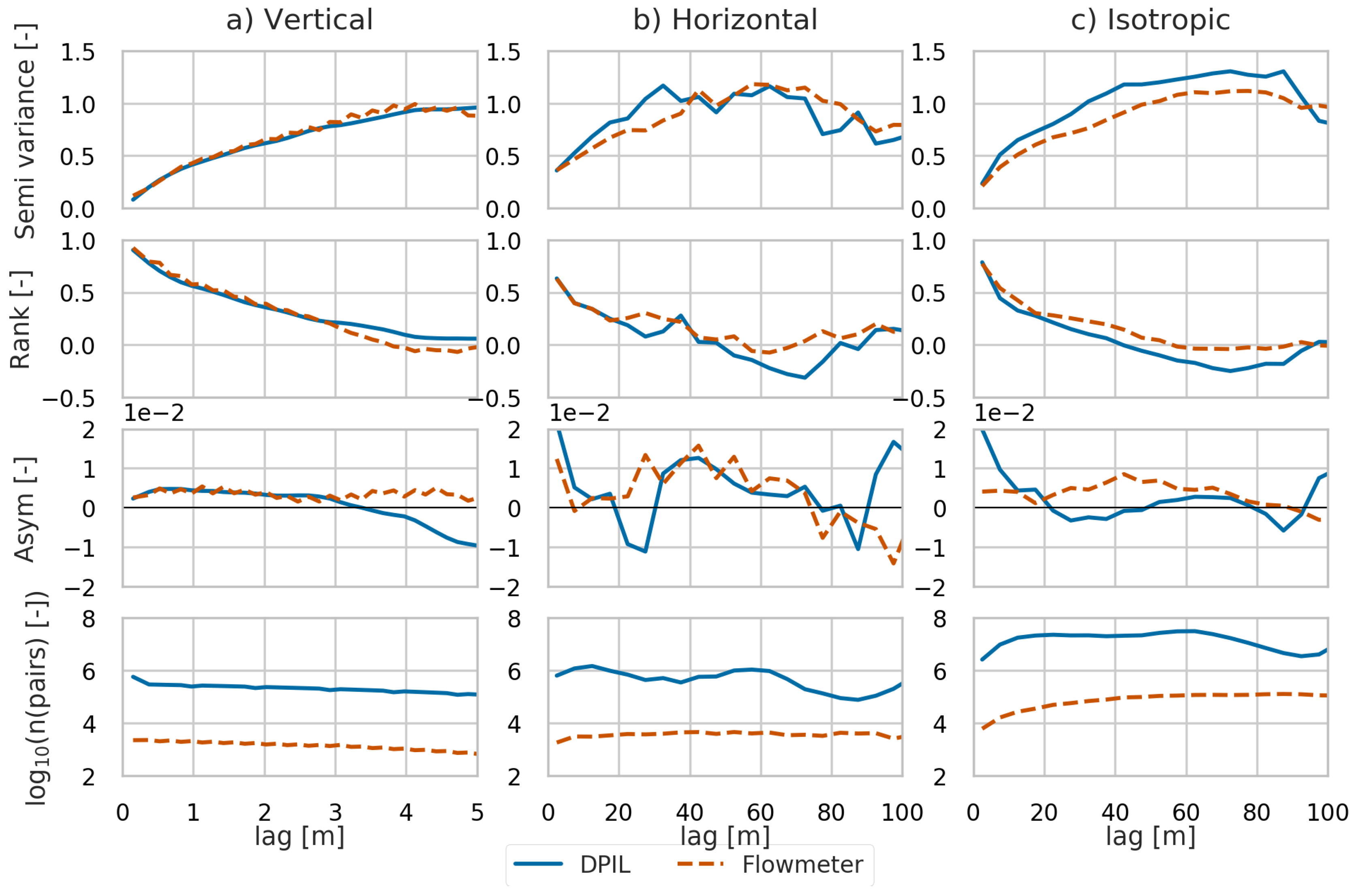
In this section, three empirical measures of spatial dependence, standardised semivariogram, rank correlation, and asymmetry (Figure 4), are analysed and compared between the DPIL and flowmeter datasets. Additionally, empirical bivariate copula densities are compared.
The spatial dependence structures have been analysed in the vertical and horizontal directions and in an equivalent isotropic coordinate system obtained by geometrically stretching the vertical axis. The directional analysis assumes azimuthal isotropy (same range for all horizontal directions), with an elliptical representation of anisotropy in the vertical plane (shortest range in the vertical direction, longest in the horizontal). Our computations of the empirical measures of spatial dependence (either the semivariogram or copula-based measures) have used the same data pair selection criteria as Rehfeldt et al. [17]. In the vertical direction, the tolerance angle is 0.1° and the tolerance bandwidth is 0.1 m so that only within-borehole data pairs (no cross-borehole pairs) contribute to the vertical measure. For the horizontal measure, a vertical tolerance angle of 5° and a vertical bandwidth of 0.16 m are used to limit the vertical separation between selected data pairs. After calculating the empirical rank correlation in the vertical and horizontal directions, the vertical to horizontal anisotropy ratio was estimated from the ranges. The data were then cast into an equivalent isotropic coordinate system by stretching the vertical axis in accordance with the estimated anisotropy ratio. In addition to the previously observed similarities [20], that we confirm, we find a systematic deviation of the measure Asym from zero, indicating a quantifiable deviance from Gaussian dependence. This will be discussed in the following part.
3.2.1. Pairwise Spatial Dependence
The vertical normalised semivariograms, and Rank and Asym measures for the two datasets are very similar (Figure 4, left column) and the equivalent isotropic versions of the semivariograms and rank correlations are also fairly similar (Figure 4, right column). Although DPIL has smoother results than flowmeter, which is influenced by the finer vertical sample spacing of the DPIL dataset. A somewhat larger difference can be found in the horizontal direction (Figure 4, central panel). This may be caused by the difference between the lateral distributions of the flowmeter and DPIL profiles. This difference can be expressed as the difference in the number of the data pairs (bottom row on Figure 4). The rank correlations between horizontal lags of 2.5 m and 17.5 m are closer to each other than are the normalised semivariograms, most likely because of the smaller impact of outliers in the rank space.
3.2.2. Asymmetry
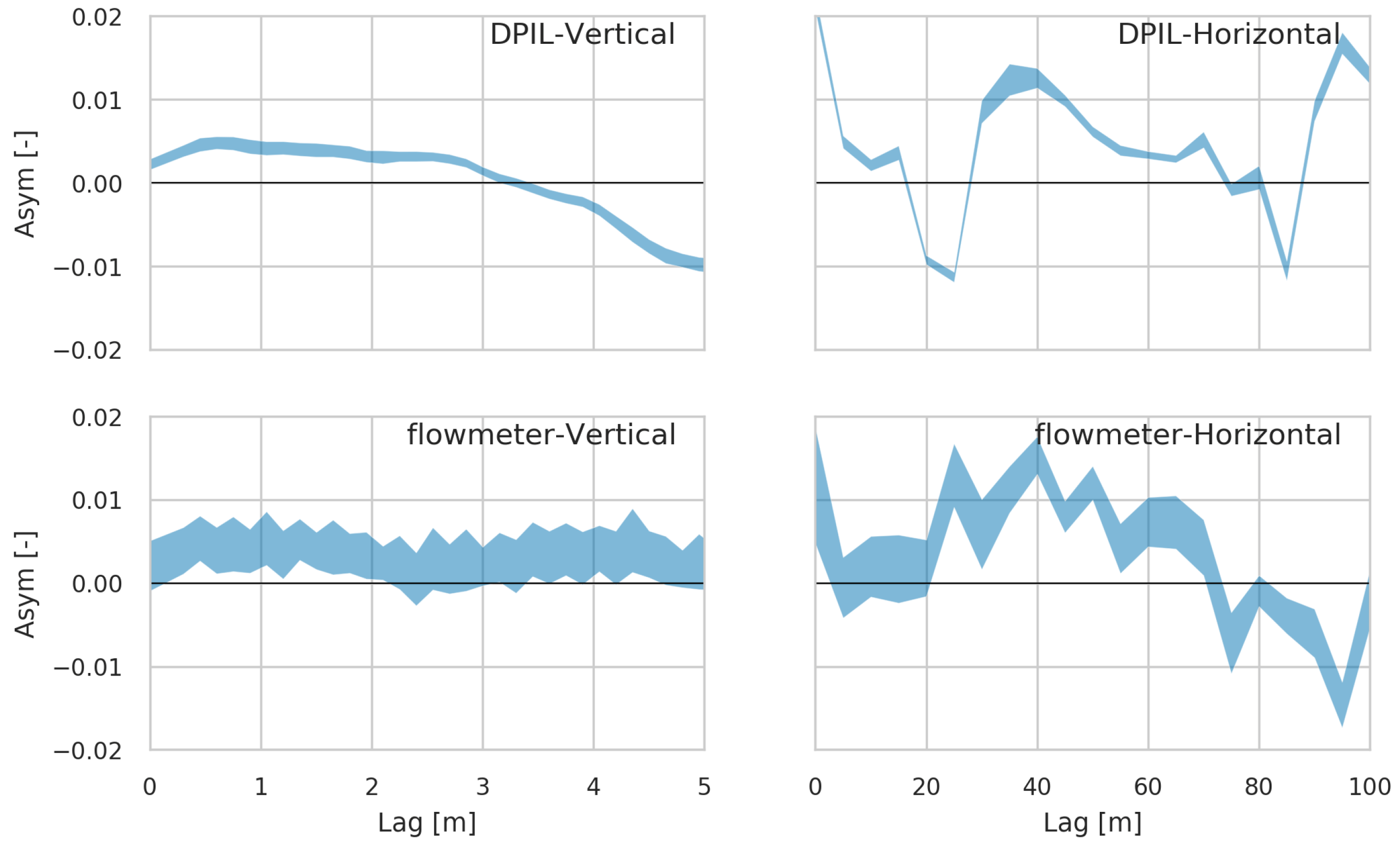
The measure Asym (third row on Figure 4) is consistently different from zero for both datasets. A bootstrap analysis, involving random selection of of the data in each realisation, indicates that the deviation from zero is consistent for each dataset (Figure 5), providing compelling evidence that the MADE site K field exhibits non-Gaussian spatial dependence. The narrower uncertainty envelopes for the DPIL results is due to the larger number of DPIL data.
In the vertical direction, the Asym values for the two datasets are essentially identical up to a lag of 3 m. For larger separation distances the Asym value of the DPIL data decreases, reaches zero at 4 m, and becomes negative beyond 4 m. In contrast, Asym remains positive for the flowmeter data. The observed behaviour of Asym indicates stronger dependence among lower K values for the DPIL dataset and among larger K values for the flowmeter dataset at large lag distances. This difference might be caused by underestimation of high K values by the DPIL and overestimation of low K values by the flowmeter [20]. Another possible reason is the difference of the distribution of the observations in the vertical direction; although the DPIL data have been trimmed to match the vertical extent of the flowmeter data sitewide [20], the vertical extents of DPIL and flowmeter profiles still differ somewhat on a local basis. This may lead to a difference of the density of higher and lower K values (Figure 3) in the two datasets, contributing to the differences in the Asym values.
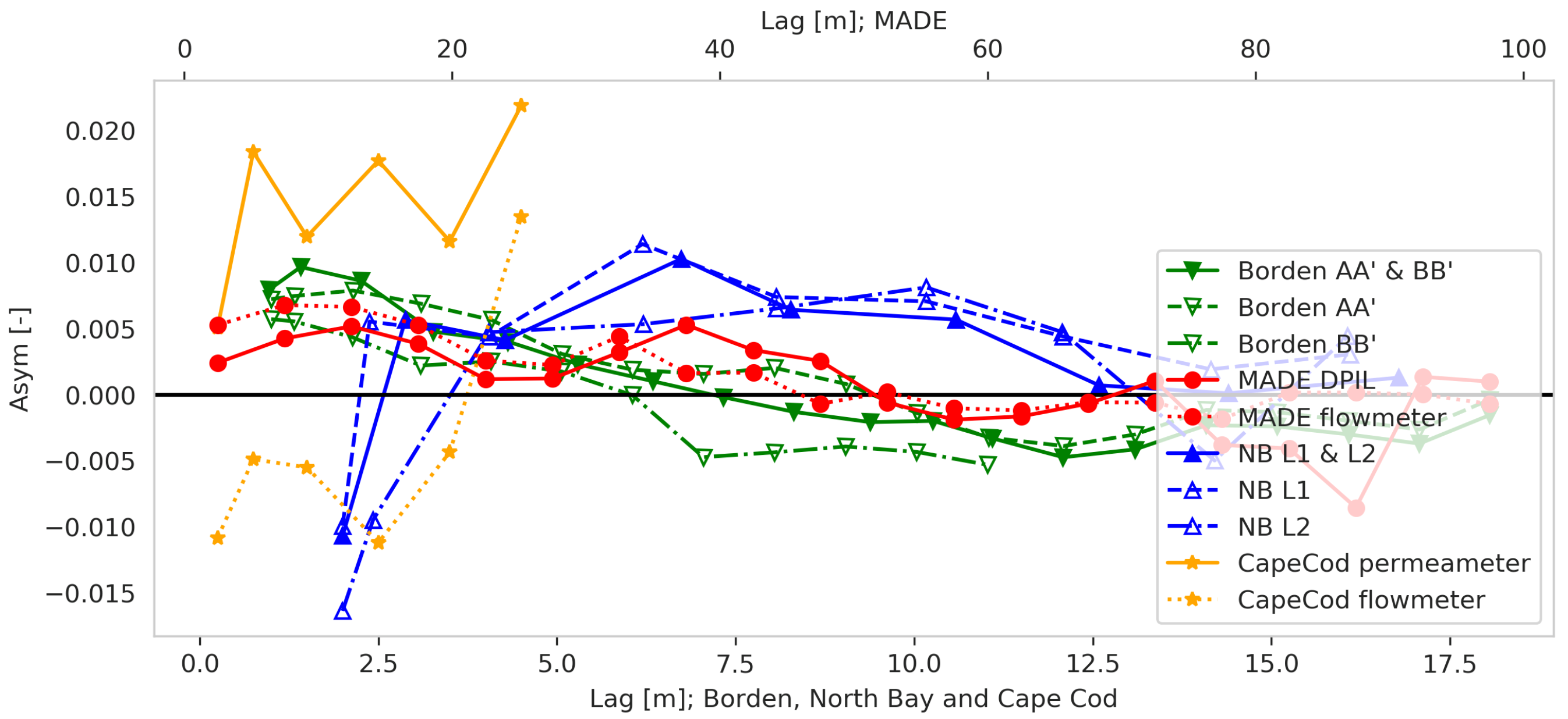
This bootstrap analysis (Figure 5) shows that is significantly different from zero at most lags for either dataset, indicating that the MADE site K field exhibits a non-symmetric, and thus non-Gaussian, spatial dependence structure. We have performed similar analyses for other well known K datasets, including those from Borden, Canada [14], Cape Cod, USA [36], and North Bay, Canada [30]. All these data-sets exhibit similar second-order dependence with different ranges (Figure 6), but the non-linear measure Asym deviates meaningfully from zero (Figure 7). In addition, many of the Asym values change sign at certain lags, indicating that for some separation distances larger K quantiles exhibit stronger spatial dependence than smaller quantiles, with the opposite behavior prevailing for other separation distances. These sign changes indicate variations in the clustering behaviour of K that are likely to influence groundwater flow and solute transport and that can not be described using two-point geostatistics.
3.2.3. Bivariate Empirical Copula Densities
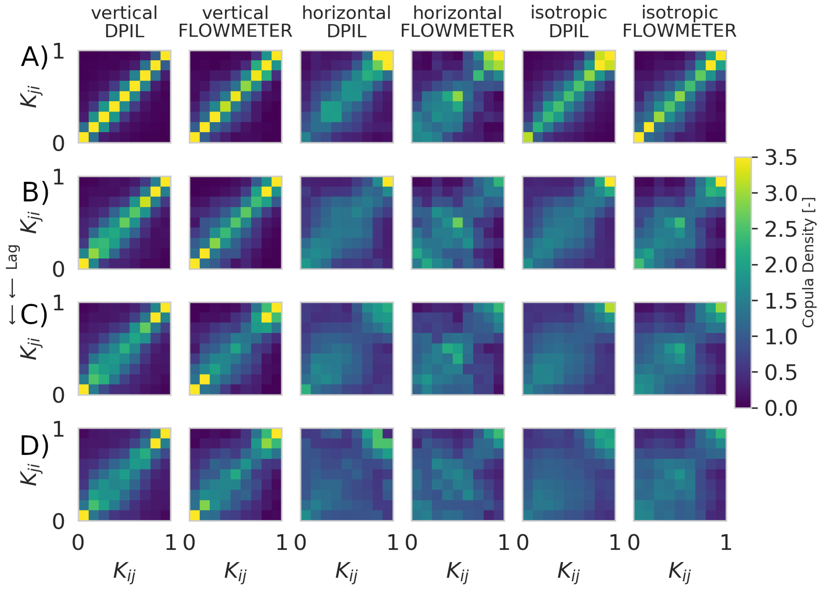
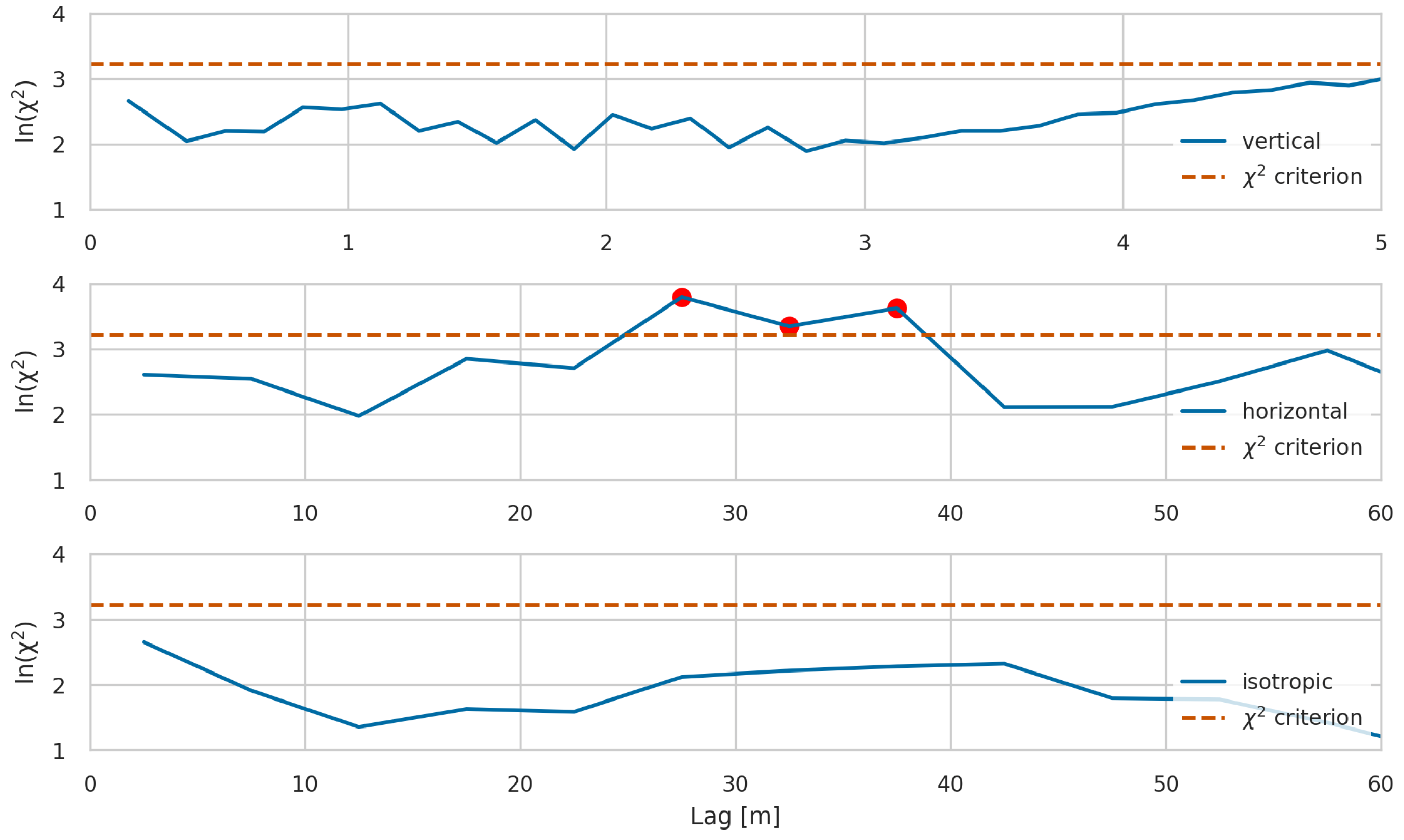
To compare the bivariate spatial dependencies of the two datasets in more detail, the empirical bivariate copula densities of the first few lag distances have been plotted (Figure 8) and a test with a significance level has been performed. The null hypothesis for this test is that the structure of the empirical bivariate copula densities of the two datasets for a certain lag distance are the same; this hypothesis is rejected if the statistic, representing the sum of squared differences between the two densities, is sufficiently large. In this case, the flowmeter and DPIL copula densities are deemed to be significantly different (the null hypothesis is rejected) only for the relatively large horizontal lag distances of 27.5 m, 32.5 m and 37.5 m (Figure 9), where data availability is an issue (fourth row on Figure 4) and that have a lesser impact on solute transport than shorter lags. For all other lags, the copula densities are are not deemed to be meaningfully different between the flowmeter and DPIL K-datasets. This is further evidence that the flowmeter and DPIL datasets exhibit similar spatial dependency structures.
Isotropic measures of dependence were calculated based on geometrically transformed coordinates. After calculation of the two directional measures, the anisotropy ratio of the two datasets can be calculated according to the results of ranges (Table 1) of the measure Rank in vertical () and in horizontal directions (). The two datasets have similar values of but different values of , which leads to different values of the anisotropy ratio, 8.18 for DPIL and 14.7 for flowmeter. Then vertical coordinates were stretched by using the anisotropy ratio to generate an isotropic dataset, such that the dataset after the transformation have identical vertical and horizontal ranges. The statistics for the each isotropic case are calculated after that. In general, the two datasets exhibit similar behaviours of the normalised semivariogram, the Rank, and Asym measures for the isotropic case.
The foregoing analysis of bivariate measures has demonstrated a strong similarity between the two datasets for short separation distances, especially in the vertical direction, along with providing compelling evidence that both datasets exhibit significantly non-Gaussian spatial dependence structures.
3.3. Results of the Copula Parameter Estimation
So far, the two datasets have been compared using empirical measures. This section compares parameter estimates for spatial dependence models for both datasets using Gauss- and v-copula models. Compared to the analysis of bivariate measures in Section 3.2, the analysis in this section is not based on pairs of data but on models with an optimised parameter vector based on ten-point subsets of the data, providing a richer representation of the spatial dependence structure than the bivariate (two-point) measures.
As mentioned in Section 1, a ML-based method was used to fit the theoretical models to randomly selected data subsets. Further details of the fitting process follow:
3.3.1. Sample Spacing
The vertical sample spacing of the DPIL measurements is one-tenth that of the flowmeter measurements. To reduce the influence of this difference on the estimated parameters, the DPIL data were averaged to the same vertical spacing as the flowmeter data prior to fitting the copula models.
3.3.2. Dimension
The parameter estimation was performed with varying numbers of data points included in each subset to provide an assessment of the effect of the subset size. The tested subset sizes were . The estimated parameter values were found to be independent of if , a finding in accordance with Bárdossy and Li [4]. Consequently, results for the smallest subset size, , are presented.
3.3.3. Parameter Vector
Besides the sill, a covariance structure of Matérn type correlation [37] with parameters range and coefficient was used. For the case with a v-copula model, there were two additional parameters: and (Equation (4)).
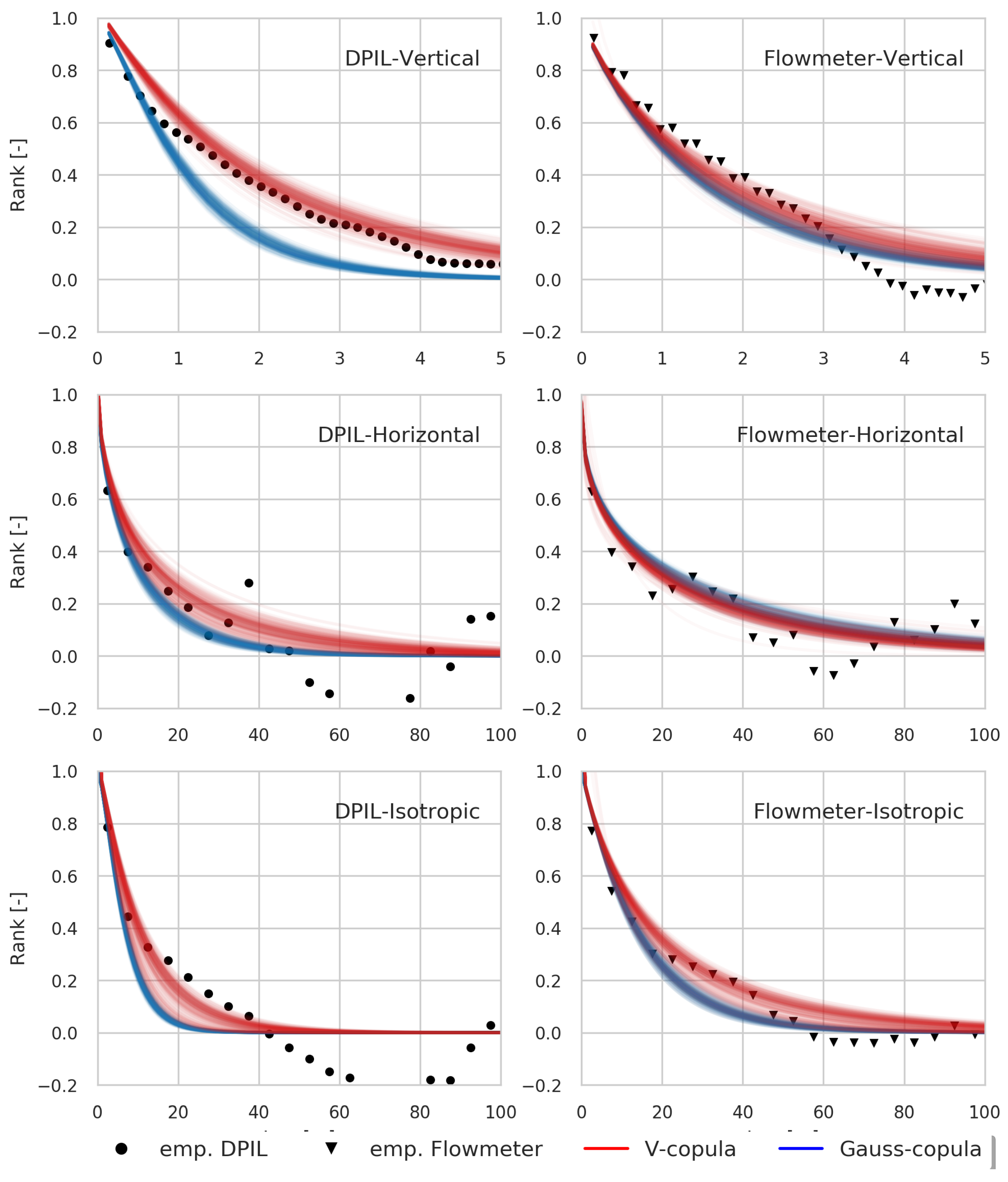
The estimated copula model parameters are shown in Table 2 and Table 3 and the model-based rank correlations computed are compared with the empirical rank correlations in Figure 10. For the v-copula estimates, the parameter is much smaller than 3.0 in all cases, indicating a non-Gaussian type of dependence. To evaluate the performance of Gauss-copula and v-copula models, Akaike information criterion ( [38], where L is the likelihood, and is the number of free parameters in the model.) is used. The estimations with a v-copula model have smaller AIC values than the estimations with a Gauss-copula model in all cases, indicating that the v-copula models provide a better fit. Compared with the rank correlations from the Gauss-copula model, the rank correlations from the v-copula model are closer to the empirical rank correlations (Figure 10). These results demonstrate the existence of non-Gaussian spatial dependence at the MADE site in high dimensions (where dimensionality here refers to the size of the data subsets). Compared with the bivariate measures in Section 3.2, these model fits show that the two datasets exhibit notable differences in higher dimensions (Table 2 and Table 3), with the following observations: (a) the flowmeter dataset exhibits a more Gaussian type of dependence than the DPIL dataset, which is indicated by the larger value of for the flowmeter data and is also apparent in Figure 10; (b) the flowmeter dataset has a smaller range in the vertical direction and larger ranges in the horizontal directionthan the equivalent isotropic case; (c) the Gauss-copula model estimates resulted in smaller ranges than the v-copula fits. The ratios of the horizontal range and the vertical range of v-copula fits (8.36 for DPIL and 14.27 for flowmeter) are closer to the empirical anisotropy ratio (Table 1) than the ratios of Gauss-copula fits (10.47 for DPIL and 18.65 for flowmeter); (d) The value of for the flowmeter data in the isotropic case is significantly different from the values estimated in the vertical and horizontal cases; (e) The diversity of the results show the uncertainty of two datasets in different directions.
Possible reasons for the observed differences in parameter estimates include: (1) The behaviour of the selected n-points subsets is influenced by varying uncertainty in the measurements of both methods and the different pattern of the measurement errors of two datasets. (2) The distribution of the measurement locations is different between the two datasets. Most notably the lateral distribution of the flowmeter profiles is more extensive and uniform than that of the DPIL profiles.
3.4. Parameter Estimation with Censored Data
Generally, we would expect any measurement method to perform optimally in a central range of measurement values and less optimally with relatively small and/or relatively large measurement values. Particularly, it has been observed in the DPIL dataset [21] that it is difficult to distinguish relatively large K values, as above a certain K value of the formation, injection-induced pressures are too small to measure accurately. For the flowmeter dataset, the lower part of the observations are influenced by a lower limit on accurate measurement of incremental flow rate [17] However, such relatively large and small K values should not be discarded, because they do carry information, namely that the unknown true value is somewhere in the interval between a threshold and the largest possible value or the lowest possible value. Such intervals can be included in estimation via maximum likelihood (Section 2.3).
We present two analyses to demonstrate the impact of accounting for data censoring in the copula analysis, one with a simulated log-normal Gaussian field to prove the concept, and one with the real MADE data sets.
In the simulation study, a 2D grid ( cells) was simulated with a known covariance structure (“truth”, marginal, mean = 10.0, standard deviation = 6.0, variogram model: ). A sample of size 2500 was generated and an independent measurement error () was added.
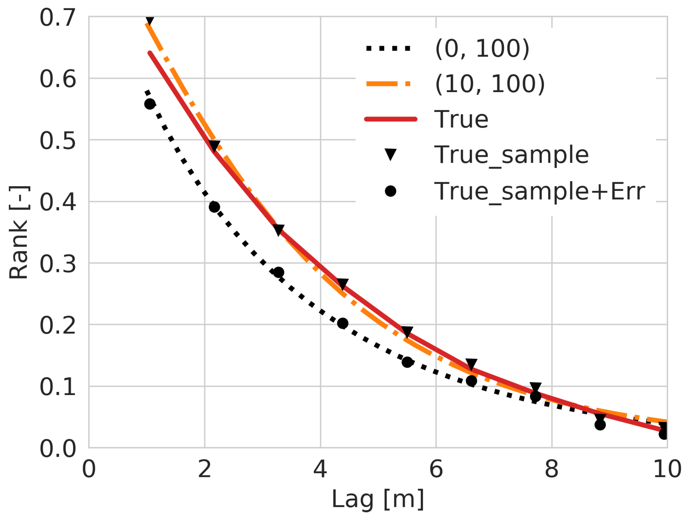
Based on this sample, parameter estimation was performed with the following scenarios: (1) the sample (with ) as fully certain, (2) the smallest , , and of the samples as being censored and parameter estimation performed using Equation (9). Scenario (2) was established, because disturbs the ranks of smaller samples more than the ranks of larger samples. Treating the smallest 10 percent of points as censored provided rank correlation estimates that were closest to thevirtual truth; this case is compared to scenario (1) (no censoring, (0, 100)) in Figure 11. This test shows that the virtual truth and the sampled data (True and True_sample) can be better estimated by including some censorship (i.e., some values below detection limit) in the copula parameter estimation when the true value is perturbed by a Gaussian error (True_sample+Err).
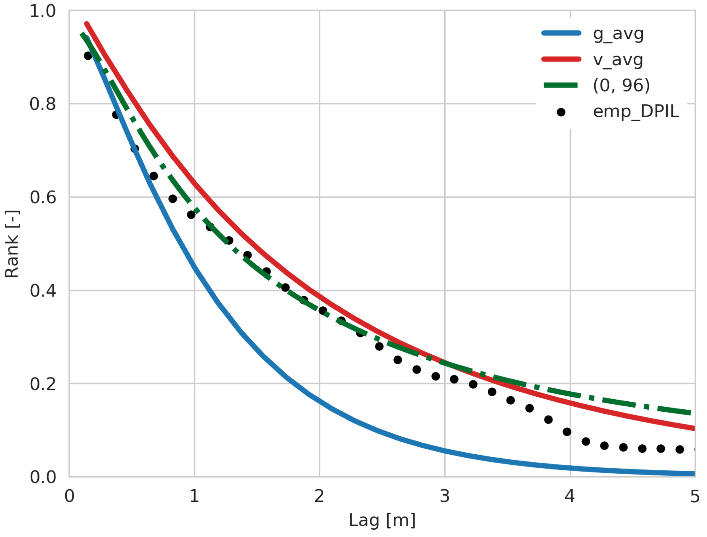
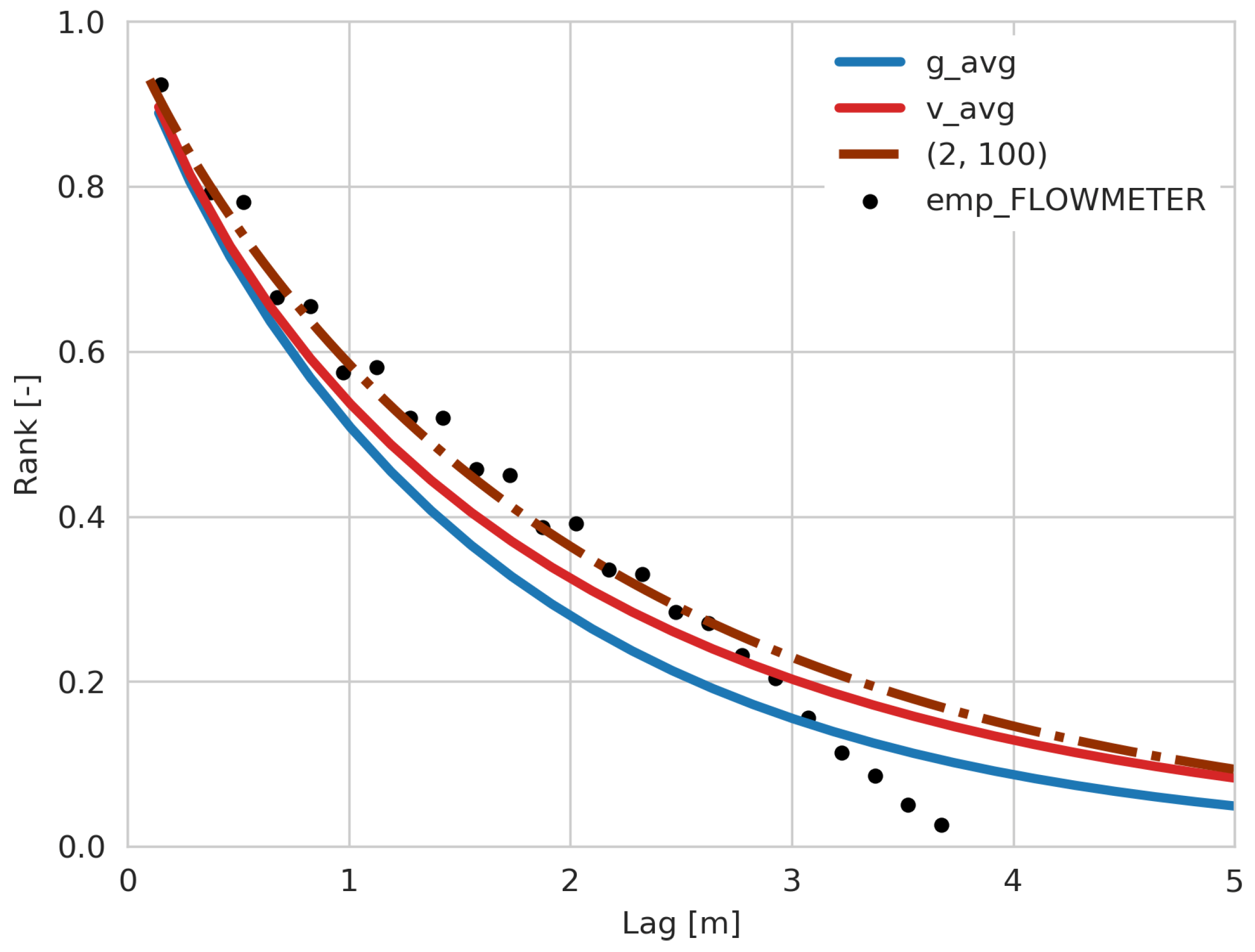
In reality, compared to the simulation case above, the true value of the rank correlation is unknown while using the MADE datasets. So the empirical rank correlation is used as the next best comparable benchmark. According to Figure 12, the empirical rank correlation can be better reproduced using the right side censoring thresholds with a censoring threshold of , which means the largest four percent observations are marked as observations with a low reliability. For the flowmeter dataset, the empirical rank correlation can be better reproduced by adding a two percent left side threshold (Figure 13). The estimated rank correlations are calculated by a Monte Carlo simulation based on the thresholds from the parameter estimation. Only very small changes were found when the thresholds were. In summary, results of parameter estimation can be improved meaningfully when at least some measurements are censored, for the flowmeter data when some small K values were treated as censored and for the DPIL data when some large K values were treated as censored.
4. Conclusions
Spatial copulas provide a novel tool to explore spatial dependence structures independently of marginal distributions. In this paper, we focused on the analysis and characterisation of the spatial dependence structures of DPIL- and flowmeter-based K measurements from the MADE site using copula-based measures.
We confirmed the similarity of the two data-sets in the marginal distribution (Figure 2) and second-order dependence measures (Figure 4 and [20]). Although in certain separation distances this similarity is influenced by the lateral coverage of two datasets (Figure 4 and Figure 9). However, we found a deviation of both data-sets from Gaussian dependence, both in (1) empirical measures and (2) mathematical models:
- The empirical measure asymmetry (Asym) systematically and within meaningful confidence intervals deviates from zero indicating that both datasets exhibit non-Gaussian dependence (Figure 4 and Figure 5). Even more, we found at the MADE site and at other relevant hydrogeologic study sites such as Borden, Cape Cod, and North Bay, that strongest dependence can exist in the small K values (Asym < 0) for some lag distances and in large K values (Asym > 0) for other lag distances (Figure 5 and Figure 7). Together with anisotropy, such a varying degree of dependence in different lag distances will lead to a meaningfully improved description of solute transport as it describes loosely speaking barriers to flow and connected high-K channels.The rank correlations of the two datasets between horizontal lags of 2.5 m and 17.5 m are more similar to each other than are the semivariogram values for these lags (Figure 4), possibly due to the reduced influence of extreme values on Rank. The datasets also have similar bivariate copula densities (Figure 8). For most lags, particularly for the short separation distances that are important when analysing solute transport behavior, the DPIL and flowmeter bivariate copula densities are not deemed to be significant differently, based on a test with a significance level of (Figure 9).
- The parameters of two different theoretical copula models were estimated to both datasets. The Gaussian model and a non-Gaussian model (v-copula) were used. The v-copula model provided a better fit to both datasets (Figure 10), indicating meaningful non-Gaussian spatial dependence.When we incorporated the uncertainty of measurements via including censored measurements below and/or above a certain threshold into the Gaussian model, the resulted parameter estimates are closer to reality than when they are not included and are also similar to estimates obtained with the v-copula model without censored measurements (Figure 12 and Figure 13).This indicates that some of the censorship properties might be mimicked by the shape of the v-copula. The ability to obtain improved Gauss-copula model fits after accounting for censoring does not conflict with the conclusion of the existence of a non-Gaussian spatial dependence, which is indicated not only by the rank correlation but also the asymmetry.The two data-sets employed are prime examples of the necessity of mimicking uncertainty related to measurements, e.g., the uncertainty of DPIL data due to the inability of the pressure transducers to accurately measure the very small injection-induced pressures that occur in high-K zones and the uncertainty of low-K in the flowmeter data due to the low flow threshold of the impeller flowmeter.
This research identified two criteria that a realistic geostatistical model for spatially distributed K-fields should fulfill: (1) it should be able to express a varying uncertainty of measurements, and (2) it should more adequately resemble the processes that lead to the spatially distributed fields. One important feature to an improved resemblance was identified to be a model that leads to both positive and negative values of the measure Asym for varying lag distances.
Author Contributions
Conceptualisation, B.X., C.H. and G.B.; Methodology, B.X., C.H. and G.B.; Software, B.X.; Formal Analysis, B.X.; Data Curation, B.X. and G.B.; Writing—Original Draft Preparation, B.X.; Writing—Review and Editing, B.X., C.H. and G.B.; Visualisation, B.X.; Supervision, C.H.; Funding Acquisition, C.H.
Funding
Funding was also received from the German Research Foundation (DFG) under project HA-7339. We thank the collaboration within the International Research Training Group “Integrated Hydrosystem Modelling” GRK 1829. The direct-push characterisation of the MADE site was supported by the Hydrologic Sciences Program of the National Science Foundation (grants EAR-0738955 and EAR-0738938).
Acknowledgments
We thank András Bárdossy for valuable discussions during our work. The MADE site direct-push data are available in Bohling et al. [21]. Further information regarding the flowmeter data can be found in [18]. The version of the flowmeter data used in this study (with the original interval K values represented as point values at interval midpoints) is available from the authors by request. We acknowledge the U.S. Geological Survey Toxic Substances Hydrology Program for sharing the data with us.
Conflicts of Interest
The authors declare no conflict of interest.
References
- Sklar, M. Fonctions de répartition à n dimensions et leurs marges; Université Paris: Paris, France, 1959; Volume 8. [Google Scholar]
- Embrechts, P.; Lindskog, F.; Mcneil, A. Chapter 8—Modelling Dependence with Copulas and Applications to Risk Management. In Handbook of Heavy Tailed Distributions in Finance; Rachev, S.T., Ed.; Handbooks in Finance; North-Holland: Amsterdam, The Netherlands, 2003; Volume 1, pp. 329–384. [Google Scholar] [CrossRef]
- Bárdossy, A. Copula-based geostatistical models for groundwater quality parameters. Water Resour. Res. 2006, 42. [Google Scholar] [CrossRef]
- Bárdossy, A.; Li, J. Geostatistical interpolation using copulas. Water Resour. Res. 2008, 44. [Google Scholar] [CrossRef]
- Marcotte, D.; Gloaguen, E. A class of spatial multivariate models based on copulas. In Proceedings of the Eighth International Geostatistics Congress, Santiago, Chile, 1–5 December 2008; pp. 177–186. [Google Scholar]
- Kazianka, H.; Pilz, J. Copula-based geostatistical modeling of continuous and discrete data including covariates. Stoch. Environ. Res. Risk Assess. 2010, 24, 661–673. [Google Scholar] [CrossRef]
- Kazianka, H.; Pilz, J. Bayesian spatial modeling and interpolation using copulas. Comput. Geosci. 2011, 37, 310–319. [Google Scholar] [CrossRef]
- Gräler, B. Modelling skewed spatial random fields through the spatial vine copula. Spat. Stat. 2014, 10, 87–102. [Google Scholar] [CrossRef] [Green Version]
- Michele, C.D.; Salvadori, G.; De Michele, C. A Generalized Pareto intensity-duration model of storm rainfall exploiting 2-Copulas. J. Geophys. Res. 2003, 108, 1–11. [Google Scholar] [CrossRef]
- Favre, A.C. Multivariate hydrological frequency analysis using copulas. Water Resour. Res. 2004, 40, 1–12. [Google Scholar] [CrossRef]
- Salvadori, G.; De Michele, C. Frequency analysis via copulas: Theoretical aspects and applications to hydrological events. Water Resour. Res. 2004, 40, 1–17. [Google Scholar] [CrossRef]
- Erhardt, T.M.; Czado, C.; Schepsmeier, U. Spatial composite likelihood inference using local C-vines. J. Multivar. Anal. 2015, 138, 74–88. [Google Scholar] [CrossRef]
- Erhardt, T.M.; Czado, C.; Schepsmeier, U. R-vine models for spatial time series with an application to daily mean temperature. Biometrics 2015, 71, 323–332. [Google Scholar] [CrossRef] [Green Version]
- Haslauer, C.P.; Guthke, P.; Brdossy, A.; Sudicky, E.A. Effects of non-Gaussian copula-based hydraulic conductivity fields on macrodispersion. Water Resour. Res. 2012, 48. [Google Scholar] [CrossRef]
- Zheng, C.; Bianchi, M.; Gorelick, S.M. Lessons learned from 25 years of research at the MADE site. Ground Water 2011, 49, 649–662. [Google Scholar] [CrossRef] [PubMed]
- Gómez-Hernández, J.J.; Butler, J.J.; Fiori, A.; Bolster, D.; Cvetkovic, V.; Dagan, G.; Hyndman, D. Introduction to special section on Modeling highly heterogeneous aquifers: Lessons learned in the last 30 years from the MADE experiments and others. Water Resour. Res. 2017, 52, 8970. [Google Scholar] [CrossRef]
- Rehfeldt, K.R.; Boggs, J.M.; Gelhar, L.W. Field Study of Dispersion in a Heterogeneous Aquifer Analysis of Hydraulic Conductivity. Water Resour. Res. 1992, 28, 3309–3324. [Google Scholar] [CrossRef]
- Boggs, J.M.; Young, S.C.; Beard, L.M.; Gelhar, L.W.; Rehfeldt, K.R.; Adams, E.E. Field study of dispersion in a heterogeneous aquifer: 1. Overview and site description. Water Resour. Res. 1992, 28, 3281–3291. [Google Scholar] [CrossRef]
- Liu, G.; Butler Jr., J.; Reboulet, E.; Knobbe, S.; Butler, J.J.; Reboulet, E.; Knobbe, S. Hydraulic conductivity profiling with direct push methods. Grundwasser 2012, 17, 19–29. [Google Scholar] [CrossRef]
- Bohling, G.C.; Liu, G.; Knobbe, S.J.; Reboulet, E.C.; Hyndman, D.W.; Dietrich, P.; Butler, J.J. Geostatistical analysis of centimeter-scale hydraulic conductivity variations at the MADE site. Water Resour. Res. 2012, 48, W02525. [Google Scholar] [CrossRef]
- Bohling, G.C.; Liu, G.; Dietrich, P.; Butler, J.J., Jr. Reassessing the MADE direct-push hydraulic conductivity data using a revised calibration procedure. Water Resour. Res. 2016, 52, WR019008. [Google Scholar] [CrossRef]
- Gilliom, R.J.; Helsel, D.R. Estimation of Distributional Parameters for Censored Trace Level Water Quality Data: 1. Estimation Techniques. Water Resour. Res. 1986, 22, 135–146. [Google Scholar] [CrossRef]
- Liu, S.; Lu, J.C.; Kolpin, D.W.; Meeker, W.Q. Analysis of Environmental Data with Censored Observations. Environ. Sci. Technol. 1997, 31, 3358–3362. [Google Scholar] [CrossRef] [Green Version]
- Cohn, T.A. Estimating contaminant loads in rivers: An application of adjusted maximum likelihood to type 1 censored data. Water Resour. Res. 2005, 41. [Google Scholar] [CrossRef]
- Bárdossy, A. Interpolation of groundwater quality parameters with some values below the detection limit. Hydrol. Earth Syst. Sci. 2011, 15, 2763–2775. [Google Scholar] [CrossRef] [Green Version]
- Haslauer, C.P.; Meyer, J.R.; Bárdossy, A.; Parker, B.L. Estimating a Representative Value and Proportion of True Zeros for Censored Analytical Data with Applications to Contaminated Site Assessment. Environ. Sci. Technol. 2017, 51, 7502–7510. [Google Scholar] [CrossRef] [PubMed]
- Harvey, C.; Gorelick, S.M. Rate-limited mass transfer or macrodispersion: Which dominates plume evolution at the macrodispersion experiment (MADE) site? Water Resour. Res. 2000, 36, 637–650. [Google Scholar] [CrossRef]
- Feehley, C.E.; Zheng, C.; Molz, F.J. A dual-domain mass transfer approach for modeling solute transport in heterogeneous aquifers: Application to the Macrodispersion Experiment (MADE) site. Water Resour. Res. 2000, 36, 2501. [Google Scholar] [CrossRef]
- Sudicky, E.A. A natural gradient experiment on solute transport in a sand aquifer: Spatial variability of hydraulic conductivity and its role in the dispersion process. Water Resour. Res. 1986, 22, 2069–2082. [Google Scholar] [CrossRef]
- Sudicky, E.A.; Illman, W.A.; Goltz, I.K.; Adams, J.J.; McLaren, R.G. Heterogeneity in hydraulic conductivity and its role on the macroscale transport of a solute plume: From measurements to a practical application of stochastic flow and transport theory. Water Resour. Res. 2010, 46. [Google Scholar] [CrossRef]
- Hess, K.M.; Wolf, S.H.; Celia, M.A. Large-scale natural gradient tracer test in sand and gravel, Cape Cod, Massachusetts: 3. Hydraulic conductivity variability and calculated macrodispersivities. Water Resour. Res. 1992, 28, 2011–2027. [Google Scholar] [CrossRef]
- Joe, H. Multivariate Models and Multivariate Dependence Concepts; CRC Press: Boca Rato, FL, USA, 1997. [Google Scholar]
- Nelsen, R.B. An Introduction to Copulas; Springer: Berlin, Germany, 2013; Volume 53, p. 276. [Google Scholar] [CrossRef]
- Joe, H. Dependence Modeling with Copulas; CRC Press: Boca Rato, FL, USA, 2014. [Google Scholar]
- Guthke, P. Non-multi-gaussian Spatial Structures: Process-driven Natural Genesis, Manifestation, Modeling Approaches, and Influences on Dependent Processes. Ph.D. Thesis, University of Stuttgart, Stuttgart, Germany, 2013. [Google Scholar]
- LeBlanc, D.R.; Garabedian, S.P.; Hess, K.M.; Gelhar, L.W.; Quadri, R.D.; Stollenwerk, K.G.; Wood, W.W. Large-scale natural gradient tracer test in sand and gravel, Cape Cod, Massachusetts: 1. Experimental design and observed tracer movement. Water Resour. Res. 1991, 27, 895–910. [Google Scholar] [CrossRef]
- Diggle, P.; Ribeiro, P.J.; Diggle, P.; Ribeiro, P.J. Model-Based Geostatistics; Springer: Berlin, Germany, 2007; p. XIII, 228 S. [Google Scholar]
- Bozdogan, H. Model selection and Akaike’s Information Criterion (AIC): The general theory and its analytical extensions. Psychometrika 1987, 52, 345–370. [Google Scholar] [CrossRef]
Figure 1.
Locations of the boreholes of DPIL (blue dots) and flowmeter (brown dots) at the MADE site.
Figure 1.
Locations of the boreholes of DPIL (blue dots) and flowmeter (brown dots) at the MADE site.

Figure 2.
CDF (upper panel) and the PDF (bottom panel) of as measured by DPIL and flowmeter analysis at the MADE site.
Figure 2.
CDF (upper panel) and the PDF (bottom panel) of as measured by DPIL and flowmeter analysis at the MADE site.

Figure 3.
Bivariate histograms of elevation Z vs. for the DPIL data-set (panel (a)) and the flowmeter data-set (panel (b)). Elevation given in meters above datum; Datum is 14.1 m below reference.
Figure 3.
Bivariate histograms of elevation Z vs. for the DPIL data-set (panel (a)) and the flowmeter data-set (panel (b)). Elevation given in meters above datum; Datum is 14.1 m below reference.

Figure 4.
Bivariate measures in the vertical direction (panel (a)), the horizontal direction (panel (b)) direction, and the isotropic case (panel (c)). From top to bottom are: normalized semivariogram, copula-based rank correlation (Rank), asymmetry (Asym), number of data pairs (n(pairs)).
Figure 4.
Bivariate measures in the vertical direction (panel (a)), the horizontal direction (panel (b)) direction, and the isotropic case (panel (c)). From top to bottom are: normalized semivariogram, copula-based rank correlation (Rank), asymmetry (Asym), number of data pairs (n(pairs)).

Figure 5.
Value areas of the copula-based asymmetry (Asym) of bootstrapping tests with random selections of the of the whole data set.
Figure 5.
Value areas of the copula-based asymmetry (Asym) of bootstrapping tests with random selections of the of the whole data set.

Figure 6.
Correlograms versus separation distance for common data-sets in stochastic hydrogeology.

Figure 7.
Asymmetries versus separation distance for common data-sets in stochastic hydrogeology.

Figure 8.
Empirical copula densities in the vertical direction (DPIL: 1st panel, flowmeter: 2nd panel), in the horizontal direction (DPIL: 3rd panel, flowmeter: 4th panel) and the isotropic case (DPIL: 5th panel, flowmeter: 6th panel). Distances from top to bottom are (A) 0.15, (B) 0.375, (C) 0.525, (D) 0.675 meter in the vertical direction and (A) 2.5, (B) 7.5, (C) 12.5, (D) 17.5 meter in the horizontal direction and the isotropic case.

Figure 9.
with a significance level 0.05 in the vertical direction (top), the horizontal direction (middle), and the isotropic case (bottom). Distances with values larger than the criterion (dash line) indicate dissimilar copula densities between two datasets (red points).
Figure 9.
with a significance level 0.05 in the vertical direction (top), the horizontal direction (middle), and the isotropic case (bottom). Distances with values larger than the criterion (dash line) indicate dissimilar copula densities between two datasets (red points).

Figure 10.
Comparison between empirical rank correlation (black dots) and the theoretical bivariate copula rank correlations of model fitting results by gauss- (blue line) and v-copula (red line) model of DPIL (left) and flowmeter dataset (right).
Figure 10.
Comparison between empirical rank correlation (black dots) and the theoretical bivariate copula rank correlations of model fitting results by gauss- (blue line) and v-copula (red line) model of DPIL (left) and flowmeter dataset (right).

Figure 11.
Comparison between the Gaussian copula parameter estimation with left side detection limit (orange dash-dotted lines with label “(10,100)”), without the detection limit (black dot line with label “(0,100)”) and the rank correlations of true domain with 10,000 points (red solid line with label “True”), a sample of the true domain with 2500 points (black inverted triangles with label “True_sample”) and the sample with a Gaussian noise (black dots with label “True_sample+Err”) by using a simulated log-normal Gaussian field.

Figure 12.
Comparison between the Gaussian copula parameter estimation with right side detection limits (dash-dotted green linewith label (0, 96)), without detection limit (solid blue line with label g_avg), v-copula parameter estimation without censored threshold (sold red line with label v_avg) and empirical rank correlation of the DPIL dataset in vertical direction (black dots with label emp_DPIL).

Figure 13.
Comparison between the Gaussian copula parameter estimation with left side detection limits (dash-dotted gray line with label (2, 100)), without detection limit (solid blue line with label g_avg), v-copula parameter estimation without censored threshold (sold red line with label v_avg) and empirical rank correlation of the flowmeter dataset in vertical direction (black dots with label emp_FLOWMETER).


Table 1.
Distances where the rank correlation is zero (range) in the vertical () and horizontal () direction and the anisotropy ratio ().
Table 1.
Distances where the rank correlation is zero (range) in the vertical () and horizontal () direction and the anisotropy ratio ().
| DPIL | 48.3 | 5.91 | 8.18 |
| flowmeter | 55.4 | 3.77 | 14.7 |
Table 2.
Representative parameter estimates for the v-copula model based on 200 randomly sampled data subsets of size 10, with the related Akaike information criterion (AIC).
Table 2.
Representative parameter estimates for the v-copula model based on 200 randomly sampled data subsets of size 10, with the related Akaike information criterion (AIC).
| Parameter | DPIL | DPIL | DPIL | Flowmeter | Flowmeter | Flowmeter |
|---|---|---|---|---|---|---|
| (Vertical) | (Horizontal) | (Isotropic) | (Vertical) | (Horizontal) | (Isotropic) | |
| v-copula [-] | 1.33 | 1.29 | 1.50 | 1.91 | 1.95 | 1.41 |
| v-copula [-] | 2.75 | 2.65 | 2.74 | 3.09 | 3.51 | 2.43 |
| Matern range [m] | 3.88 | 34.57 | 17.09 | 3.12 | 44.53 | 40.92 |
| Matern [-] | 0.71 | 0.34 | 0.79 | 0.43 | 0.20 | 0.45 |
| AIC [-] | −5562.87 | −3166.46 | −4901.32 | −2969.11 | −1598.68 | −2805.82 |
Table 3.
Representative parameter estimates for the Gauss-copula model based on 200 randomly sampled data subsets of size 10, with the related Akaike information criterion (AIC).
Table 3.
Representative parameter estimates for the Gauss-copula model based on 200 randomly sampled data subsets of size 10, with the related Akaike information criterion (AIC).
| Parameter | DPIL | DPIL | DPIL | Flowmeter | Flowmeter | Flowmeter |
|---|---|---|---|---|---|---|
| (Vertical) | (Horizontal) | (Isotropic) | (Vertical) | (Horizontal) | (Isotropic) | |
| Matern range [m] | 1.51 | 15.81 | 8.95 | 2.31 | 43.08 | 20.78 |
| Matern [-] | 0.79 | 0.29 | 0.94 | 0.42 | 0.18 | 0.50 |
| AIC [-] | −5183.33 | −2951.80 | −4697.32 | −2929.49 | −1558.70 | −2762.78 |
© 2019 by the authors. Licensee MDPI, Basel, Switzerland. This article is an open access article distributed under the terms and conditions of the Creative Commons Attribution (CC BY) license (http://creativecommons.org/licenses/by/4.0/).
Share and Cite
MDPI and ACS Style
Xiao, B.; Haslauer, C.; Bohling, G. Comparison of Multivariate Spatial Dependence Structures of DPIL and Flowmeter Hydraulic Conductivity Data Sets at the MADE Site. Water 2019, 11, 1420. https://doi.org/10.3390/w11071420
AMA Style
Xiao B, Haslauer C, Bohling G. Comparison of Multivariate Spatial Dependence Structures of DPIL and Flowmeter Hydraulic Conductivity Data Sets at the MADE Site. Water. 2019; 11(7):1420. https://doi.org/10.3390/w11071420
Chicago/Turabian StyleXiao, Bo, Claus Haslauer, and Geoffrey Bohling. 2019. "Comparison of Multivariate Spatial Dependence Structures of DPIL and Flowmeter Hydraulic Conductivity Data Sets at the MADE Site" Water 11, no. 7: 1420. https://doi.org/10.3390/w11071420
Note that from the first issue of 2016, this journal uses article numbers instead of page numbers. See further details here.