Microturbines at Drinking Water Tanks Fed by Gravity Pipelines: A Method and Excel Tool for Maximizing Annual Energy Generation Based on Historical Tank Outflow Data

Abstract

Wherever the flow of water in a gravity pipeline is regulated by a pressure control valve, hydraulic energy in the form of water pressure can instead be converted into useful mechanical and electrical energy via a turbine. Two classes of potential turbine sites exist—those with (class 1, “buffered”) and those without (class 2, “non-buffered”) a storage tank that decouples inflow from outflow, allowing the inflow regime to be modified to better suit turbine operation. A new method and Excel tool (freely downloadable, at no cost) were developed for determining the optimal hydraulic parameters of a turbine at class 1 sites that maximize annual energy generation. The method assumes a single microturbine with a narrow operating range and determines the optimal design flow rate based on the characteristic site curve and a historical time series of outflow data from the tank, simulating tank operation with a numerical model as it creates a new inflow regime. While no direct alternative methods could be found in the scientific literature or on the internet, three hypothetically applicable methods were gleaned from the German guidelines (published by the German Technical and Scientific Association for Gas and Water (DVGW)) and used as a basis of comparison. The tool and alternative methods were tested for nine sites in Germany.

1. Introduction

1.1. Advantages and Characteristics of Potential Drinking Water Hydropower Facilities

Hydropower is among the renewable energy sources with the best life-cycle energy balance—the ratio between the energy output (e.g., electricity) and the energy input required to manufacture, install, operate and dispose of the infrastructure and equipment needed for energy generation [1,2]. Drinking water hydropower has further advantages compared to much larger hydropower facilities at dams, weirs and run-of-river schemes, including high water quality (enabling long lifetime and low-maintenance operation), minimal to no environmental impact (due to a previously existing, closed system) and relatively good economic viability [2,3,4]. Thanks to technological progress, capitalizing on drinking water hydropower potential is increasingly becoming economically viable even at the bottom of the capacity spectrum, below 10 kW of available hydraulic power [4,5,6,7,8,9]. Practical methods and easy-to-use design tools play an important role in facilitating the implementation of such projects.

A gravity pipeline is the central element of most drinking water hydropower schemes, connecting a higher-elevation water source to lower-elevation water storage tanks and water users. With respect to hydropower development, there are two relevant types of gravity pipelines: those with and those without pressure control at points downstream, such as transfer stations or outlets into storage tanks. Gravity pipelines with pressure control valves can be thought of as possessing “surplus” potential energy, which can be “harvested” by using a turbine rather than “wasted” by using a pressure control valve, which “throttles” the flow of water (see Appendix A.1 for more background on gravity pipelines and the hydraulic explanation for surplus energy).

There are two main classes of eligible turbine sites for drinking water hydropower (as illustrated by Figure 1), in which the flow rate is either

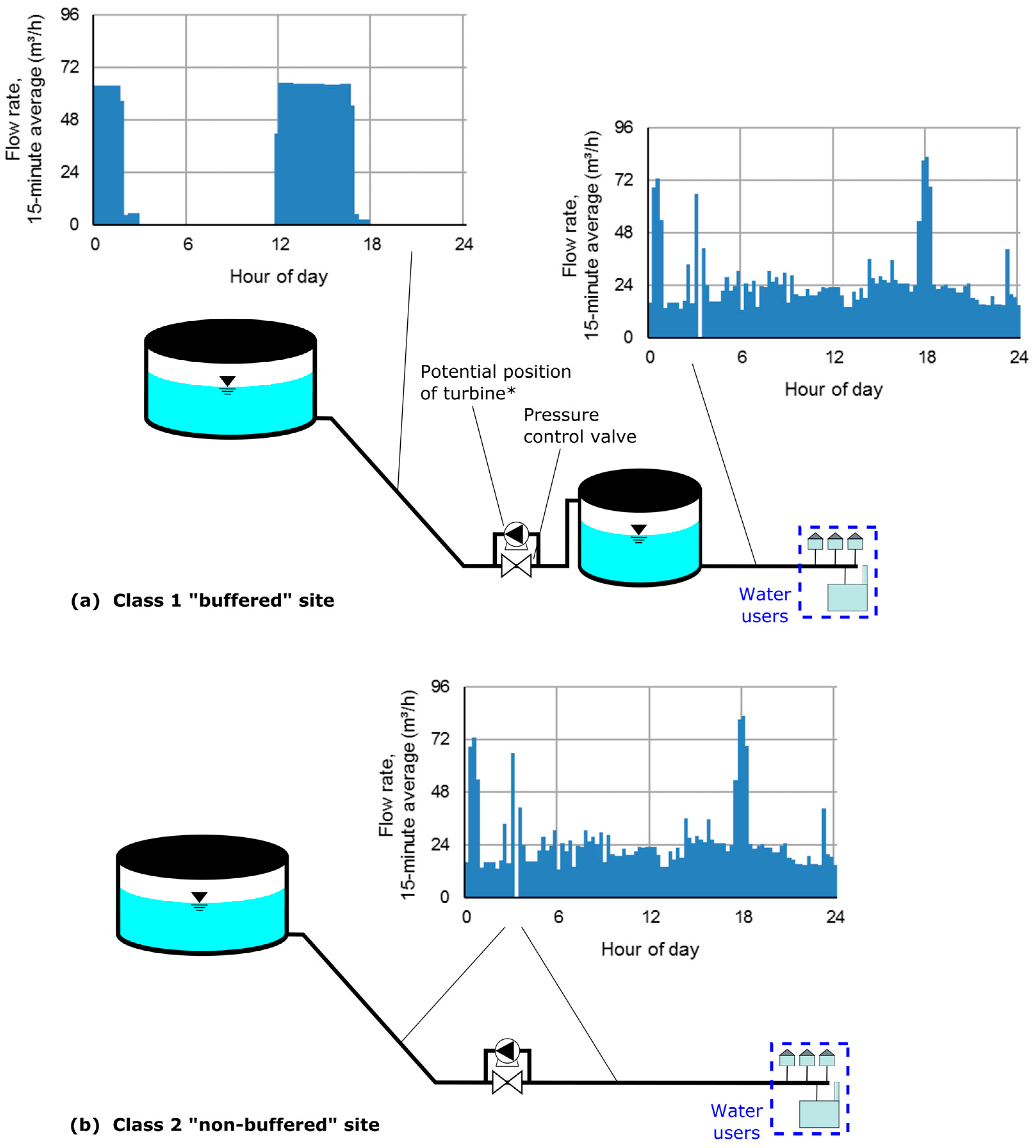
• decoupled from uncontrolled downstream water use through a storage tank (“buffered”), or
• determined by uncontrolled water use in the downstream supply zone(s) (“non-buffered”).

Table 1. Matrix of consequences for drinking water hydropower development, depending on the type of gravity pipeline and site.

	Water Supply Site	with Storage Tank (Class 1, “Buffered“)	without Storage Tank (Class 2, “Non-Buffered”)
Gravity Pipeline
with pressure control		Hydropower is very practical, as the storage tank provides flexibility in re-defining the inflow regime	Hydropower is possible, but may require a complex design to accommodate high variability in flow rate and pressure due to uncontrolled downstream water use
without pressure control		Hydropower is theoretically possible, but would reduce inflow rate if installed at outlet of existing pipeline, which may negatively affect supply reliability

summarizes the most relevant consequences for drinking water hydropower development that follow from the presence or absence of pressure control and a storage tank. As sites without pre-existing pressure control are not promising for hydropower development, they will not be further considered in this paper.

1.2. Available Literature and Comparison of Class 1 vs. Class 2 Sites

Common examples of class 2 sites include transfer nodes between pressure zones or a gravity-fed water treatment plant between a gravity source and destination supply tank (e.g., [2,5,8,10,11,12]). They are most often located within the water “distribution” section of the water supply chain [13]. In contrast to class 1 sites, class 2 sites offer no flexibility in the choice of flow rate, such that a turbine must be designed to efficiently operate over a broad spectrum of flow rates and corresponding available pressure heads. As the pressure may fluctuate both downstream and upstream of the turbine installation site, class 2 sites generally require more information and a more complex, customized design process. Based on a review of the scientific literature, the authors perceive a dominant focus on class 2 sites, with many researchers devising design algorithms and control solutions using microturbines and pumps-as-turbines (PATs) [7,8,9,13,14,15,16,17,18,19,20,21,22].

Class 1 sites are generally intermediate (such as break-pressure tanks (BPTs)) or terminal storage tanks with pressure control valves [6], typically located within the water “transmission” section of the water supply chain [13]. In the authors’ experience and estimation, class 1 sites are common and represent a relatively cost-effective opportunity for renewable energy generation. They offer the water supplier flexibility (positively correlated with storage volume) in determining the rate, duration and timing of tank filling (and thus turbine operation), as this must not necessarily occur simultaneously with the downstream use in the supply zone (see Figure 1). Assuming that the inflow rate is not restricted (e.g., by the naturally occurring, seasonally varying flow from a mountain spring), the inflow regime can often be freely adjusted to maximize energy generation through a turbine, regardless of how it was managed in the past [12].

While comparatively less common, there are also studies that focus on class 1 sites. Several authors present case studies of sites at the bottom of dams [7], spring-fed pipelines [23] and storage tanks in general [24,25]. Others focus on BPTs, both isolated [6] and in series along a long-range pipeline [26,27]. However, many if not all of these authors effectively treat class 1 sites as if they were class 2 sites, assuming that the inflow regime remains unchanged and attempting to design turbines to fit this inflow regime, rather than adjusting it to allow the choice of a single, optimized turbine. Thus, they do not use the fundamental technical advantage that separates class 1 from class 2 sites [12,28]. For more background on class 1 vs. class 2 sites, see Appendix A.3.

1.3. Filling a Gap in Currently Available Design Methods for Class 1 Sites

Several other authors present methods that might be useful for class 1 sites, but the effort required to successfully adapt the methods and restrictions imposed by technical understanding and software availability for the authors’ intended user group (practitioners at water supply companies and non-research water professionals) speak against pursuing this further. For instance, since the authors set out to create a tool that is free to use and based on a common tool (i.e., Microsoft Excel, which in the authors’ experience is standard practice at most water supply companies), and software such as MATLAB is non-standard and requires specialized knowledge, possible adaptation of such algorithms was not considered. Furthermore, while some authors provide the basic underlying equations, the software or code in which the algorithms are implemented is not made accessible to the reader and therefore cannot be easily tested or used.

The 2016 guidelines published by the German Technical and Scientific Association for Gas and Water (DVGW) [12] identify the flexibility advantage provided by class 1 “buffered” sites, and imply that with additional data analysis a turbine can be “ideally tuned” to “balance the demands of storage management and energy generation”. However, they offer no specific instructions or examples for how to translate this information into actual design parameters (flow rate and pressure drop). This is precisely the gap that the authors intend to fill with the method and accompanying Excel tool presented here. As the authors of this paper have encountered many class 1 sites and experienced an unfulfilled need for a design solution, they decided to develop their own solution. While designing turbine systems for class 2 sites represents the greater technical challenge, a practical design method for class 1 sites appears to be low-hanging fruit that has yet to be sufficiently plucked.

Given a recently resurging interest in drinking water hydropower in Germany [29,30,31,32] and elsewhere [6,7,19], the authors intend to facilitate the installation of such facilities by making it easier for small and medium water suppliers to estimate their hydropower potential and perform the basic design (determination of turbine parameters) themselves. The tool is implemented in Microsoft Excel for Windows (Office 2010 or newer), available free of cost for download at the authors’ university website [33] and intended to be easily useable by practicing engineers or water professionals. If successful, it should both save time and reduce users’ inhibitions about approaching this non-standard topic. To the authors’ knowledge, it is the only such tool freely available on the internet.

This paper will explain the methodology behind the Excel tool, along with three other methods covered in DVGW guidelines that serve as a useful basis of comparison. These four methods will be applied to nine sites in Germany, and the results will be used to show the method in practice as well as providing a sense of the technical and economic potential that is available at class 1 drinking water hydropower sites.

2. Materials and Methods

2.1. Design Premise

The intention of this method and related Excel tool is to facilitate the implementation of microturbines in water supply systems. This is accomplished by automating the calculations required to determine the pressure head and flow rate for a hypothetical turbine that will (to the fullest extent possible with the given data) lead to the maximum electrical energy generation (kWh/annum, or kWh/a) at a given class 1 site. A basic economic analysis is also performed to provide an estimate of the project’s viability.

While the Excel tool includes four calculation options to accommodate all anticipated variations on data availability for a given site (see Appendix B.1 and Appendix B.2 for a more detailed explanation), optimization of the turbine design parameters is only possible using option 1 or 2 (both slight variants on the same method), which take historical flow data into account. The primary advantage of options 1 and 2 is that there is no need to be biased by the typical inflow regime of past operations. The analysis of historical data thus allows the determination of turbine parameters from “first principles”, rather than by analogy from the previous inflow rate, which may have been selected for reasons unknown to the current responsible engineer or site operator. Critically, this assumes that historic water use patterns are a reliable proxy for future water use. This paper will present the main design algorithm for calculation options 1 and 2 in its recommended form. The tool provides some additional options for the user to customize the design solution (e.g., regarding the bypass flow rate and multipliers for the outflow rate (Q_out) to reflect anticipated future changes), which are further described in Appendix B.3 and Appendix B.4 and the tool itself.

This method was inspired by Haakh [28], who provided a foundational and mathematically thorough treatment of turbine and pump operation in the context of water supply systems. The authors expect that the Excel tool and this article will provide a somewhat simplified, more user-friendly approach to solving a sub-set of the design challenges laid out there, with a focus on class 1 “buffered” sites. The following sections describe the essential tasks performed by the tool.

2.2. Determining the Characteristic Site Curve

Also known as the “system” curve, this describes the relationship between the exerted pressure and flow rate in the inflow pipeline as observed from a downstream reference point within the pipeline. It can also be thought of as the pressure “available” as a function of the chosen flow rate. Typically, this reference point is taken just upstream of the pressure control valve, to capture the hydraulic conditions relevant for a potential turbine. The available pressure head is equal to the maximum pressure head (h_max, at flow rate = 0) minus the head loss up to the point of interest (h_loss) and the pressure head just downstream of the control valve (h_downstream)_, which is necessary for the water to reach the storage tank. Since head loss increases proportionally to the square of flow rate, the curve can be well approximated (Equation (1)) with a downward-facing parabola with its vertex centered on the positive y-axis (flow rate = 0), crossing the positive x-axis at the maximum possible flow rate (pressure exerted on reference point upstream of valve = 0), at which the pressure control valve is completely open and offers no hydraulic resistance (see Figure 8 in Section 3.1 for an example). This is predicated on a simplifying assumption that assumes a constant coefficient of major pipe friction loss (defined in the U.S. as “lambda”, λ), which is known to be flow rate-dependent (e.g., as captured in Moody’s diagram), but is valid for conditions commonly encountered at water supply sites. The resulting second-order polynomial equation takes the following form:

$$h_{available} \left(m\right)= h_{max}- K_{loss}·Q^2-h_{downstream}$$

(1)

where K_loss is the head loss coefficient, which integrates the major head loss due to pipe friction and minor head loss(es) due to sources of local resistance (e.g., pipe bends, partially opened valves upstream). h_loss as defined in Figure A1 (Appendix A.1) is the central term in Equation (1), the product of K_loss with the square of the flow rate Q. While h_max, K_loss and h_downstream could be determined analytically, the authors found empirical determination to be both more accurate and less labor-intensive. To empirically determine this parabolic curve, two points must be defined, which requires measuring five field data points:

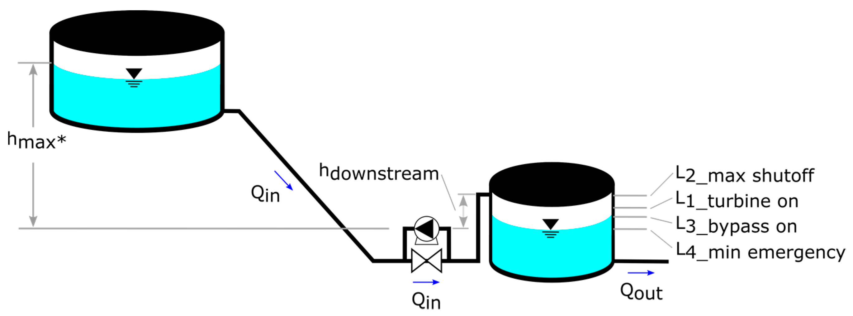
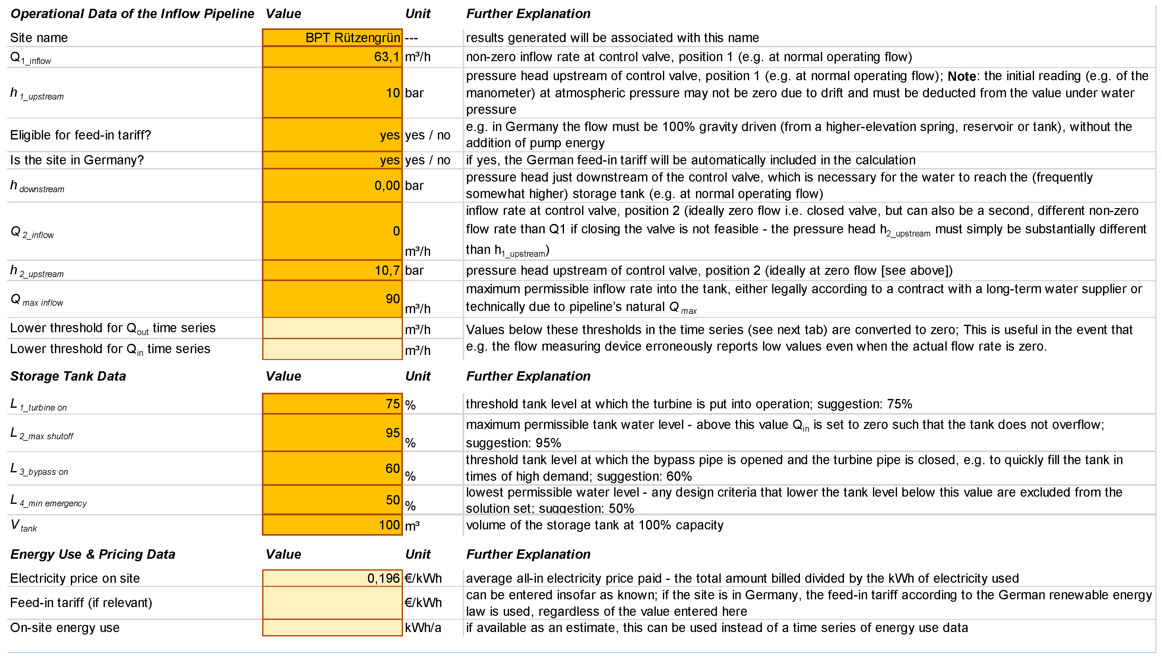
• Q_{1_inflow}: non-zero inflow rate at control valve, position 1 (e.g., at normal operating flow)
• h_{1_upstream}: pressure head upstream of control valve, position 1 (e.g., at normal operating flow)
• h_downstream: pressure head just downstream of the control valve, which is necessary for the water to reach the (frequently somewhat higher) storage tank (e.g., at normal operating flow)
• Q_{2_inflow}: inflow rate at control valve, position 2 (ideally zero flow; i.e., closed valve, but can also be a second, sufficiently different non-zero flow rate than Q₁, if closing the valve is not feasible)
• h_{2_upstream}: pressure head upstream of control valve, position 2 (ideally at zero flow; see above)

These data can usually be easily obtained, for example during a 30-min visit to a site or based on past data already acquired using a supervisory control and data acquisition (SCADA) system. If feasible, long-term measurements as well as further points along the site curve provide a more accurate picture of the real site conditions and reduce uncertainty in the resulting turbine performance. Since K_loss can effectively be considered a constant, it can be determined indirectly by substituting all measured values into Equation (1). Q_max can then be determined simply by setting Equation (1) to zero and solving for Q (Equation (2)).

$$Q_{max}= \sqrt{\frac{h_{max}-h_{downstream}}{K_{loss}} }$$

(2)

The reader should note that the timing of the measurement of h_{1_upstream} and h_{2_upstream} will impact the value of h_max, since the pressure measured depends to a small degree on the water level in the upstream tank. Ideally, these measurements should be conducted when the upstream tank is known to be at its typical lowest level, as this will provide a conservative estimate of the pressure that will at a minimum be reliably available to a potential turbine. Furthermore, the flow-dependent head losses between the control valve and storage tank are integrated into the measurement of h_downstream, if performed using a pressure gauge. The change in these losses (and therefore a change in h_downstream) due to a deviation in the turbine flow rate from Q_{1_inflow} (normal operating flow) is likely negligible, but can also be easily measured by changing the flow rate to the potential future turbine flow rate. The value for h_downstream is usually primarily determined either by the height of the pipe outlet above the turbine (as portrayed in Figure 2) or the water level in the downstream tank (as portrayed in Figure A1), in case the pipe outlet is at the bottom of the downstream tank. Figure 2 provides a visual explanation of some of these terms for the typical case as encountered by the authors in Germany.

2.3. Calculating the Hydraulic Power Available to the Turbine

The hydraulic power carried by the flowing, pressurized water and ultimately available to a turbine can be calculated using Equation (3):

$$P_{hydraulic} \left(kW\right)= \rho ·g·Q·h_{available}·1000$$

(3)

where ρ is the density of water (kg/m³), g is gravitational acceleration (m/s²), Q is the flow rate (m³/s) and h_available is the available pressure head (m). Since ρ and g can be assumed constant (1000 kg/m³ and 9.81 m/s², respectively), the equation can be simplified (Equations (4a) and (4b)) to allow the input of flow rate in more commonly used units of m³/h or L/min:

$$P_{hydraulic} \left(kW\right)= \frac{Q·h_{available}}{367},\mathrm{with}Q\mathrm{in}{\mathrm{m}}^3/\mathrm{h}$$

(4a)

$$P_{hydraulic} \left(kW\right)= \frac{Q·h_{available}}{6116},\mathrm{with}Q\mathrm{in}\mathrm{L}/\min$$

(4b)

Given that h_available is approximated as a second-order polynomial function of Q (Equation (3)), and this function is multiplied with Q and a constant to compute available hydraulic power, the characteristic curve of hydraulic power available to a turbine can therefore be approximated as a third-order polynomial function of Q (Equation (5)), adjusted by the appropriate constant as per Equation (4):

$$P_{available} \left(kW\right)=\left(h_{max}·Q- K_{loss}·Q^3-h_{downstream}·Q\right) / 367,\mathrm{with}Q\mathrm{in}{\mathrm{m}}^3/\mathrm{h}$$

(5)

The flow rate at which the maximum possible hydraulic power P_max occurs can be determined by first taking the derivative of Equation (5) with respect to flow rate Q, resulting in Equation (6):

$$P{\prime }_{available} \left(kW\right)=\left(h_{max}- 3·K_{loss}·Q^2-h_{downstream}\right) / 367,\mathrm{with}Q\mathrm{in}{\mathrm{m}}^3/\mathrm{h}$$

(6)

Since Equation (5) defines a polynomial with a single maximum, setting its derivative P’_available to zero leads to Equation (7) for the flow rate corresponding to P_max:

$$Q_{P\_max} ({\mathrm{m}}^3/\mathrm{h})=\sqrt{\frac{h_{max}-h_{downstream}}{3·K_{loss}} }$$

(7)

Substituting Q_{P_max} into Equation (5) yields the maximum possible hydraulic power for the given class 1 site. This information becomes relevant upon comparing the results of this method with the method from the 1994 DVGW guidelines [34] (see Section 2.10).

2.4. Consideration of a Bypass Pipeline Parallel to the Turbine

The tool assumes that the turbine is installed in the inflow pipeline to the storage tank and in parallel with a bypass. This ensures at a minimum that the turbine can be easily removed without interrupting supply and can also be used for the compensation of short periods of high water demand via rapid filling of the storage tank. In the event that the bypass flow rate Q_bypass is substantially above the turbine design flow rate Q_turbine, this can maximize total annual energy generation, by enabling Q_turbine to be as low possible, which reduces unnecessary friction losses that would otherwise occur with a higher Q_turbine. This relationship between Q_bypass and Q_turbine should become clearer in the coming sections. The recommended setting is the maximum permissible inflow rate, but this can be freely adjusted by the user.

2.5. Using a Numerical Model to Ensure Supply Reliability Based on Historical Flow Data

The inflow rate Q_in must at any point in time be sufficient to meet the demand placed on the storage tank by the water users in the supply zone and cannot endanger the reliability of supply by causing the storage tank to temporarily run below a minimum emergency level (e.g., for fire-fighting reserves). To determine whether this is likely to happen based on a given Q_bypass and Q_turbine, a simple linear, deterministic, dynamic numerical model was incorporated into the tool. The model takes a historical time series of the outflow rate from the storage tank Q_out as input (ideally at a maximum time interval of 15 min) and simulates Q_in through the turbine and bypass as well as the resulting storage tank water level L_tank. The initial condition for L_tank is 75% if no water level time series data are provided along with the time series for Q_out. The basic governing equation (Equation (8)) for L_tank at a given timestamp t+1 is as follows:

$$L_{tank @ t+1} \left(\% of full\right)=L_{tank @ t}+\frac{\left(V_{in @ T} - V_{out @ T}\right)}{V_{tank} · 100}$$

(8)

where L_{tank @ t+1} reflects the resulting tank water level at timestamp t+1 at the end of the time step T (between timestamps t and t+1), V_{in @ T} and V_{out @ T} are the volume of water entering and leaving the tank during the time step T (between timestamps t and t + 1), respectively, and V_tank is the volume of the storage tank at 100% capacity (m³). To clarify, “timestamp” t refers to an instantaneous point in time (e.g., 12:00:00 (noon) on 20 June 2019), whereas “time step” T refers to the duration of time passing between the two timestamps t and t+1 (e.g., the 15 min between 12:00:00 and 12:15:00). V_out and V_in are obtained by multiplying the duration of the time step T ([t + 1] − t) with Q_out and Q_in, respectively, to yield a water volume. Q_out is taken from the historical time series provided by the user, whereas Q_in is determined by Equation (9):

$$Q_{in @ t+1}=\{\begin{array}{ll}{Q}_{bypass},& \mathit{i}\mathit{f} \left(L_{tank @ t}\le L_{2_{\max shutoff}} \mathit{a}\mathit{n}\mathit{d} Q_{in @ t}=Q_{bypass}\right)\\ & \mathit{e}\mathit{l}\mathit{s}\mathit{e}\mathit{i}\mathit{f} L_{tank @ t}\le L_{3_{bypass}on}\\ Q_{turbine} ,& \mathit{i}\mathit{f} L_{tank @ t}\le L_{1_{turbine}on }\\ 0,& \mathit{i}\mathit{f} L_{tank @ t}>L_{2\_max shutoff}\end{array}$$

(9)

where Q_bypass is the chosen bypass flow rate, Q_turbine is the chosen turbine flow rate, L_{2_max shutoff} is the maximum permissible tank water level (% of full), L_{1_turbine on} is the threshold tank level at which the turbine is operated, L_{3_bypass on} is the threshold tank level at which the bypass pipe is opened, and the turbine pipe is closed. A further value, L_{4_min emergency}, signifies the lowest permissible water level. If L_tank falls short of this, the Q_turbine is excluded from the set of feasible solutions. See Figure 2 for a visual representation of these tank levels. For the method to properly function, the following relationships between values must be true (Equations (10a) and (10b)):

L_{2_max shutoff} > L_{1_turbine on} > L_{3_bypass on} > L_{4_min emergency}

(10a)

Q_{max inflow} ≥ Q_bypass ≥ Q_turbine

(10b)

where Q_{max inflow} is the maximum permissible inflow rate into the tank, either legally according to a contract with a long-term water supplier or technically due to pipeline’s natural Q_max (see Appendix A.1 for elaboration) or a limitation on the water source (e.g., a mountain spring). The recommended setting is for Q_turbine to be equal to Q_{max inflow}.

Expressed in words, the system is operated such that the tank is normally filled via the turbine at Q_turbine. Only in cases of high water withdrawal (Q_out) in which the tank level falls very rapidly is the bypass opened (and the turbine pipe closed) to increase the inflow rate to Q_bypass and kept open until the maximum permissible water level is exceeded (tank is full). Then normal operation with the turbine resumes. The number of occasions on which the bypass is opened increases as Q_turbine decreases.

By defining Q_in to exclusively be equal to Q_turbine and Q_bypass, taking into account the impact on L_tank, the tool thus re-defines the inflow regime in such a way that both supply reliability can be guaranteed, and energy generation can be maximized (see Figure 1). This is the step in the tool’s algorithm at which the key advantage of class 1 “buffered” sites is utilized.

2.6. Calculating Total Annual Hydraulic Energy Capture

The term “capture” refers to the annual average amount of hydraulic energy E_hydraulic that is applied to the turbine wheel, before being converted to the mechanical energy E_mechanical of the spinning wheel and shaft, and then further converted to electrical energy E_electrical through a generator. E_hydraulic is calculated using Equation (11):

$$E_{hydraulic} \left(\frac{kWh}{a}\right)=\frac{{{\displaystyle \sum }}_t^{t_{max}-1}\{\begin{array}{cc}{P}_{hydraulic}\left(Q_{turbine}\right)·\left(\left(t+1\right)-t\right)·24 h/d ,& \mathit{i}\mathit{f} Q_{in @ t}=Q_{turbine}\\ 0,& \mathit{i}\mathit{f} Q_{in @ t}\ne Q_{turbine}\end{array}}{\left(\frac{t_{max}-t}{365 d/a}\right)}$$

(11)

where the time step ([t + 1] – t) is measured in units of days (standard for Microsoft Excel). The resulting Q_in at each timestamp t (Equation (9)) depends on the outcome of the numerical model described above. This model therefore performs two functions: (1) calculating the energy production for each time step and (2) monitoring whether the water level falls below the minimum permissible level in the storage tank and flagging such solutions as invalid.

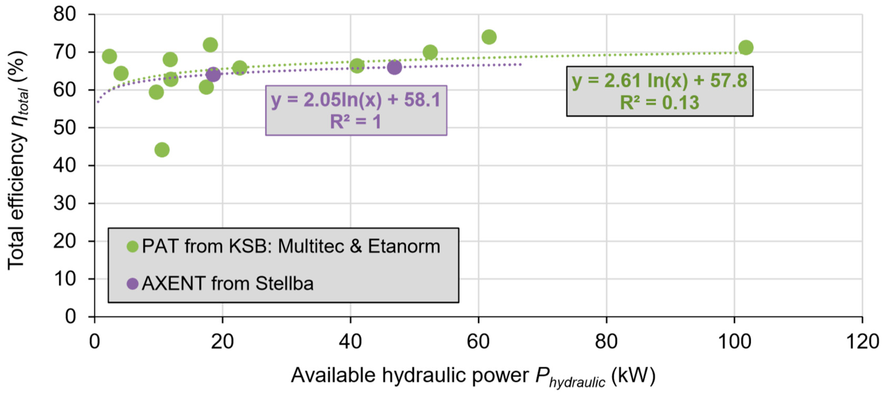
2.7. Selection of Microturbines, Global Efficiency Curves and Calculating Total Annual Electric Energy Generation

The tool assumes a single turbine having only a narrow operating range with acceptable efficiency. The turbine’s characteristic resistance curve is assumed constant, since it is fixed by the frequency of the electrical power connection (presumed to be grid electricity at 50 or 60 Hz) and the number of pole pairs in the electrical generator, which pre-determine the rotational speed of the turbine.

To provide the tool user with the calculated electrical energy generation, it is necessary to estimate the total efficiency, which is a product of the efficiency of the turbine (hydraulic to mechanical energy) and efficiency of the generator (mechanical to electrical energy). To make the tool as appealing as possible to practicing engineers, the authors chose to use data from two microturbines that are currently on the market: the in-line axial “AXENT” turbine from Stellba Hydro [35] and pumps-as-turbines (PAT) from KSB [36], companies with whom the authors have worked previously. The total efficiency η_total at the hydraulic best efficiency point for turbines of varying capacities was plotted relative to P_hydraulic, leading to Figure 3. For each type, AXENT and PAT (two separate models), natural log curves were fitted to the data to generate equations that enabled the estimation of η_total based on the input of P_hydraulic (Equations (12a) and (12b)). The tool can be updated with new data for other types of turbines from other companies, although this cannot currently be easily done by a normal user.

$${\eta }_{total} (\%)=2.05·\ln \left(P_{hydraulic}\right)+58.1\left(\mathrm{AXENT}\right)$$

(12a)

$${\eta }_{total} (\%)=2.61·\ln \left(P_{hydraulic}\right)+57.8\left(\mathrm{PAT}\right)$$

(12b)

It is important to note that the curves in Figure 3 represent the global efficiency curve of single, optimal values of η_total for a hypothetical range of different turbines, not the characteristic efficiency curve of a single turbine over its operating range. Each turbine also has its own flow-dependent efficiency, such that the operating efficiency will vary from the optimal η_total in the event that it is operated off of its design flow rate, or if a turbine cannot be manufactured to have its peak efficiency precisely at the chosen Q_turbine. For simplicity’s sake, the tool assumes that the turbine is only operated at its optimal η_total, at a single operating point. The flow rate must be high enough to enable the use of a microturbine with a practical size and sufficiently high efficiency, as the efficiency of turbines and generators drops rapidly with declining physical dimensions.

The total annual electrical energy generation E_electrical for a given Q_turbine and choice of turbine type is then determined by Equation (13):

$$E_{electrical} \left(\frac{kWh}{a}\right)= E_{hydraulic}·{\eta }_{total}$$

(13)

2.8. Iteratively Determining the Optimal Turbine Design Parameters

The optimal turbine parameters are defined in the tool as the combination of Q and h that lead to the greatest annual electrical energy generation in kWh/a, based on a numerical simulation of turbine operation with the historical Q_out data provided by the user (see above). Generally speaking, a longer historical time series produces more reliable results by accounting for a wider range of realistic supply scenarios, but a very long time series runs the risk of using obsolete data that does not reflect the expected future supply scenarios and therefore producing sub-optimal results. In the authors’ experience, 12 to 24 months is ideal.

To determine the optimal parameters, the possible solution space of values for Q_turbine is iteratively run through the numerical model, calculating E_electrical for each value of Q_turbine. This is first done at intervals of 5 m³/h to determine the approximate optimal Q_turbine, and then again at intervals of 0.5 m³/h to refine this result. The Q_turbine leading to the greatest E_electrical is declared optimal, and the corresponding h_turbine calculated using Equation (1).

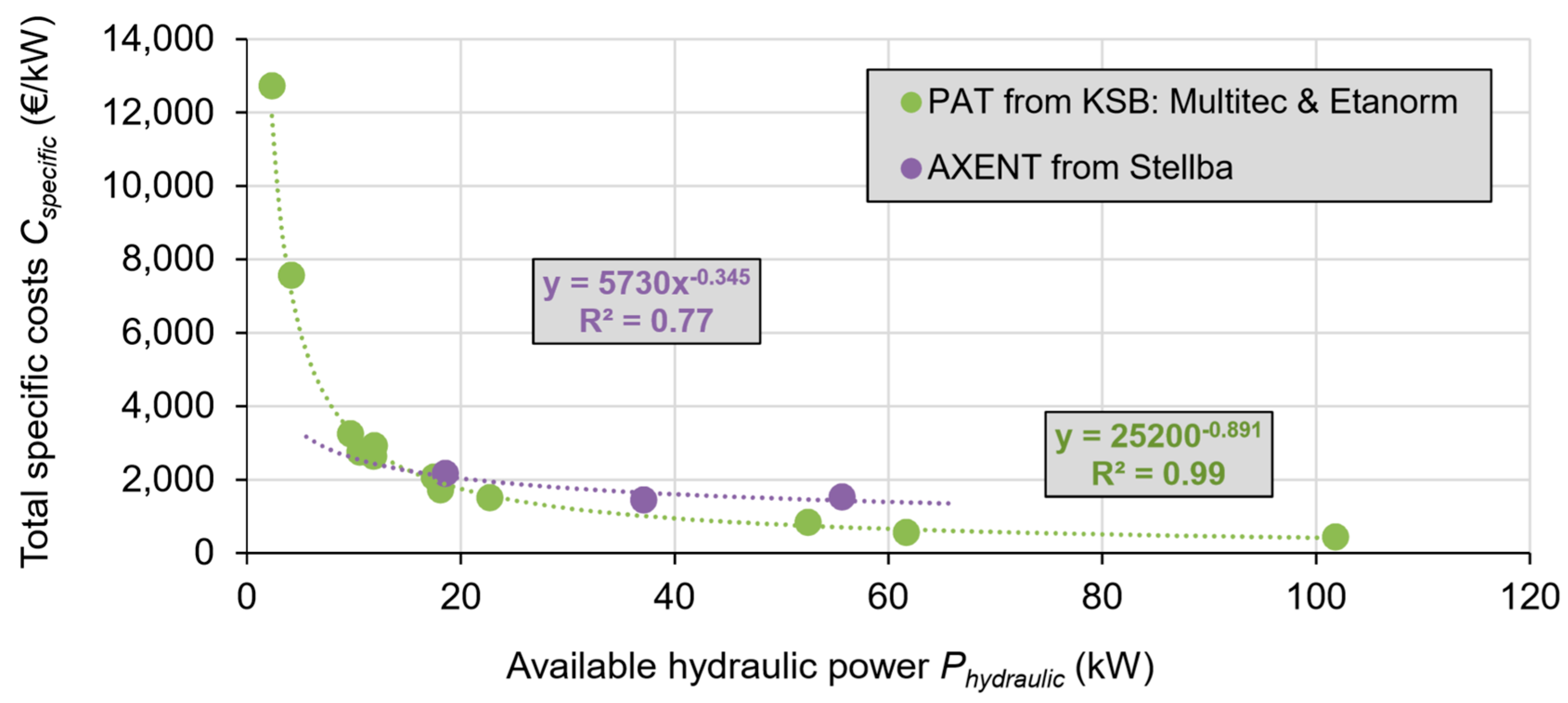
2.9. Estimating Economic Viability

Similar to the determination of η_total, the estimation of economic viability is based on available cost data for actual microturbines from the companies Stellba and KSB. These costs are based on past implemented projects, recent price quotes and the experience of collaborating engineers, and include the cost of purchase, installation and commissioning.

Table 2. Summary of cost parameters for AXENT turbines and PATs.

	Cost Parameter	Purchase Cost (Turbine and Generator)	Installation	Pipe Modi-fications	Electromechanical Control Systems	Total Incl. 19% Value-Added Tax (VAT)
Turbine Type
AXENT (Stellba)		27,500–65,000 €	2500–4000 €	1500–3000 €	1000 €	40,500–85,700 €
PAT (KSB): Multitec and Etanorm		4400–15,700 €	5000–8000 €	5000 €	10,000 €	29,100–46,100 €
Data source (year)		Past invoice and recent price quotes (2016–2018)	Past projects (2011–2016) and engineering estimates (2016–2018)

shows the cost items and the ranges for the two different types of turbines incorporated into the tool, as well as the total costs including the 19% value-added tax (VAT) for Germany. The peripheral costs for the AXENT turbine are generally lower, because the design elements required to install it are less complex, and it does not require protection against pressure shocks (water “hammer”), contrary to a typical PAT. Figure 4 shows the specific total cost C_specific data for both types of turbines.

Equations (14a) and (14b) show the specific cost function for each turbine type. The shape of these curves corresponds approximately to data compiled from turbine projects in Switzerland [1]. The total specific costs C_specific are calculated by entering P_hydraulic into Equations (14a) and (14b), and the total costs C_total for a given site and turbine are obtained by multiplying P_hydraulic with C_specific.

$${\mathrm{C}}_{specific} \left(€/k{W}_{hydraulic}\right)=5730·P_{hydraulic}{}^{-0.345}(\mathrm{AXENT},\mathrm{Stellba})$$

(14a)

$${\mathrm{C}}_{specific} \left(€/k{W}_{hydraulic}\right)=25200·P_{hydraulic}{}^{-0.891}(\mathrm{PAT},\mathrm{KSB})$$

(14b)

The annual benefits B_annual are based on user input on the applicable feed-in tariff or other electricity price at which the generated energy could be sold. In Germany, for example, the legally guaranteed feed-in tariff for turbines below a total capacity of 100 kW commissioned in 2019 is 12.27 ct. €/kWh, for a contract length of 20 years. A site is only eligible for this tariff if the water flows via gravity from its natural source to the turbine. Otherwise, the energy must normally be used on site, replacing electrical energy that would otherwise been purchased from the grid, in Germany at a price of approximately 20 ct. €/kWh. The tool combines the estimated benefits from both of these sources (Equation (15)), which can also complement each other (e.g., if there is a pump set that can be occasionally but not continuously supplied with energy by the turbine, or if the turbine is only able to cover a portion of the energy demand of the pumps).

$$B_{annual} \left(\raisebox{1ex}{$€$}\!\left/ \!\raisebox{-1ex}{$a$}\right.\right)=\sum \{\begin{array}{ll}{E}_{electrical}·Pric{e}_{grid electricity}& \mathit{i}\mathit{f} E_{electrical} coincides with grid energy use\\ E_{electrical}·Pric{e}_{feed-in tariff}& \mathit{i}\mathit{f} E_{electrical} \sout{coincides} with grid energy use\\ & \mathit{a}\mathit{n}\mathit{d} site eligible for a feed-in tariff\end{array}$$

(15)

The payback period for the project is calculated in a simple manner by comparing the initial costs and annual benefits to each other (Equation (16)), assuming the energy generation remains unchanged and without taking into account the time-dependent value of money. Depending on the tool user and decision-maker, the payback period can serve as an indicator of economic viability, if necessary complemented by consideration of C_total, as many projects are hindered by insufficient initial funding.

$$Payback period \left(a\right)= \frac{C_{total} (€)}{B_{annual} \left(€/a\right)}$$

(16)

2.10. DVGW 1994 and 2016 Methods as a Basis of Comparison

In order to provide a frame of reference for the new method, it is compared to three methods available in the 1994 and 2016 editions of the DVGW guidelines published on the topic of energy recovery through turbines in the drinking water supply. While these guidelines provide a very useful overview of the technical and operational aspects of implementing a drinking water hydropower project, these methods are not known to generate optimal design solutions for class 1 sites, and therefore only serve as a frame of reference for the new method being introduced here. The methods are compared based on the parameter E_electrical in units of kWh/a.

The most recent edition of the DVGW guidelines [12] provides guidance in the case of class 2 “non-buffered” sites. They suggest using a frequency distribution of the occurring flow rates to determine the design flow rate of the turbine or multiple turbines. The flow rate (or mean of a range of flow rates; e.g., 52.5 m³/h representing the range from 50 to 55 m³/h) having the greatest energy density (result of Equation (17), applied to each range of flow rates) should be the design turbine flow rate. The resulting Q_turbine is then given as input into the Excel tool to calculate E_electrical assuming the inflow regime is modified as with the tool’s optimization algorithm. In this way, this method is evaluated more generously than if it were applied as intended to class 2 sites, since the flow rates occurring above and below the chosen Q_turbine would not contribute to energy generation, being too high or low to be efficiently processed by the turbine (see Section 3.2 and Table 4 for a concrete example).

$$E_{hydraulic} \left(\frac{kWh}{a}\right)=\frac{{{\displaystyle \sum }}_t^{t_{max}-1}\{\begin{array}{c}{P}_{hydraulic}\left(Q_{range mean}\right)·\left(\left(t+1\right)-t\right)·24\frac{h}{d}, \mathit{i}\mathit{f} Q_{range min} < Q_{turbine} \le Q_{range max}\\ 0, \mathit{i}\mathit{f} Q_{turbine} \le Q_{range min} \mathit{o}\mathit{r} Q_{turbine} > Q_{range max}\end{array}}{\left(\frac{t_{max}-t}{365 d/a}\right)}$$

(17)

This method is divided into two sub-methods, one based on the Q_in into the tank (approximately representing the “status quo”, if the inflow regime were not modified), and the other based on Q_out from the tank. Historical time series are required for both in order to apply Equation (17).

The original edition of the DVGW guidelines [34] make no distinction between class 1 and 2 sites and suggests using the historically most frequently occurring flow rate to select the turbine. However, they imply that the theoretical optimal flow rate is given by Equation (18) (obtained by substituting Equation (2) into Equation (7)), at which the hydraulic power carried by the flowing water is mathematically at its maximum (see also [28,37]).

$$Q_{P\_max}=\frac{1}{\sqrt{3}}·Q_{max}=0.577·Q_{max}$$

(18)

This method is tested on the basis of the flow rate of maximum hydraulic power. Just as for the 2016 DVGW method, the resulting Q_turbine is given as input into the Excel tool to calculate E_electrical assuming the inflow regime is modified as with the tool’s optimization algorithm.

Table 3. Summary of turbine design methods from the authors’ perspective.

	Turbine Design	(1) HTWD 1 2018	(2) DVGW 2 1994	(3) DVGW 2016, a 3	(4) DVGW 2016, b 4
Method Characteristics
Basis for design		Diverse data to determine the flow rate with the maximum annual energy generation	Q with max. hydraulic power (see Equation (18))	Qout	Qin
				with historically greatest energy density (see Equation (17))
Data requirements		Medium to high	Lowest	Medium
Confidence of achieving max. energy generation		Highest (with high data reqs.)	Lowest	Low to medium

¹ HTWD — Hochschule für Technik und Wirtschaft Dresden (University of Applied Sciences), the authors’ home institute; ² DVGW — Deutscher Verein des Gas- und Wasserfaches (German Technical and Scientific Association for Gas and Water), publisher of guidelines on drinking water hydropower; ³ a—variant of the DVGW method based on tank outflow; ⁴ b—variant of the DVGW method based on tank inflow

offers a concise summary of all methods that are compared in this paper with their corresponding short names.

3. Results

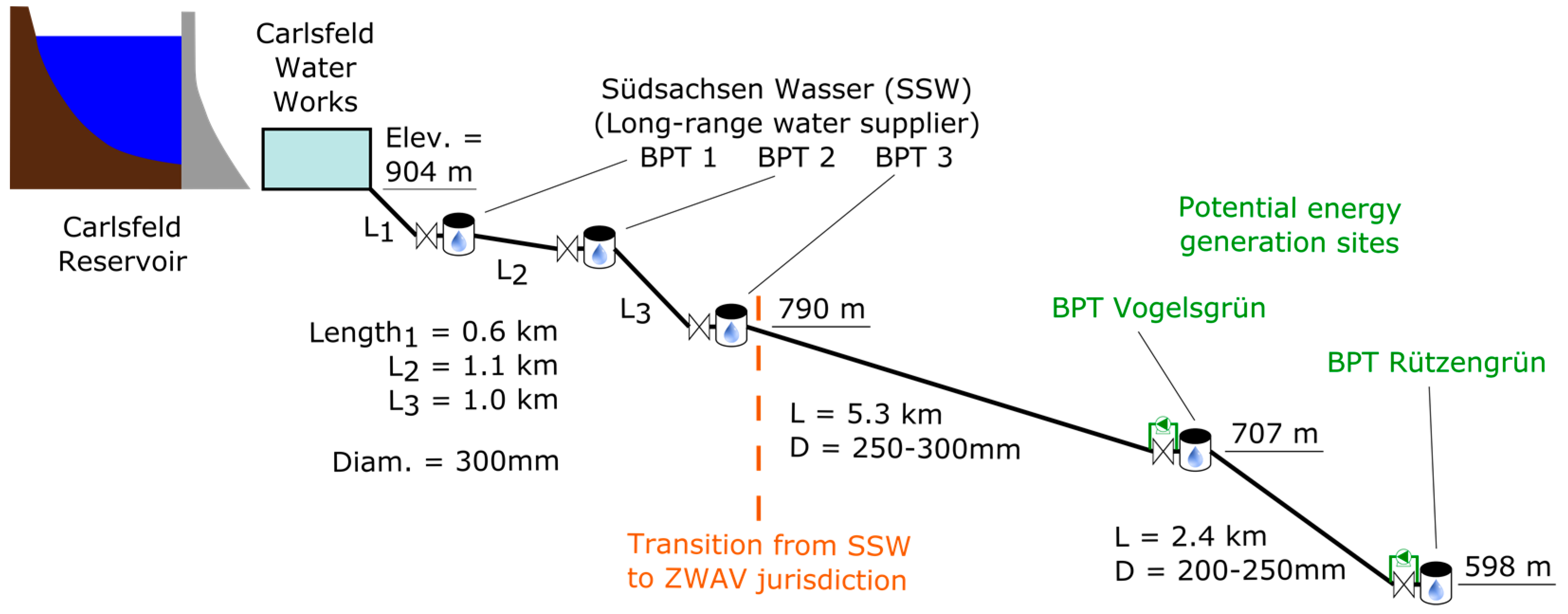
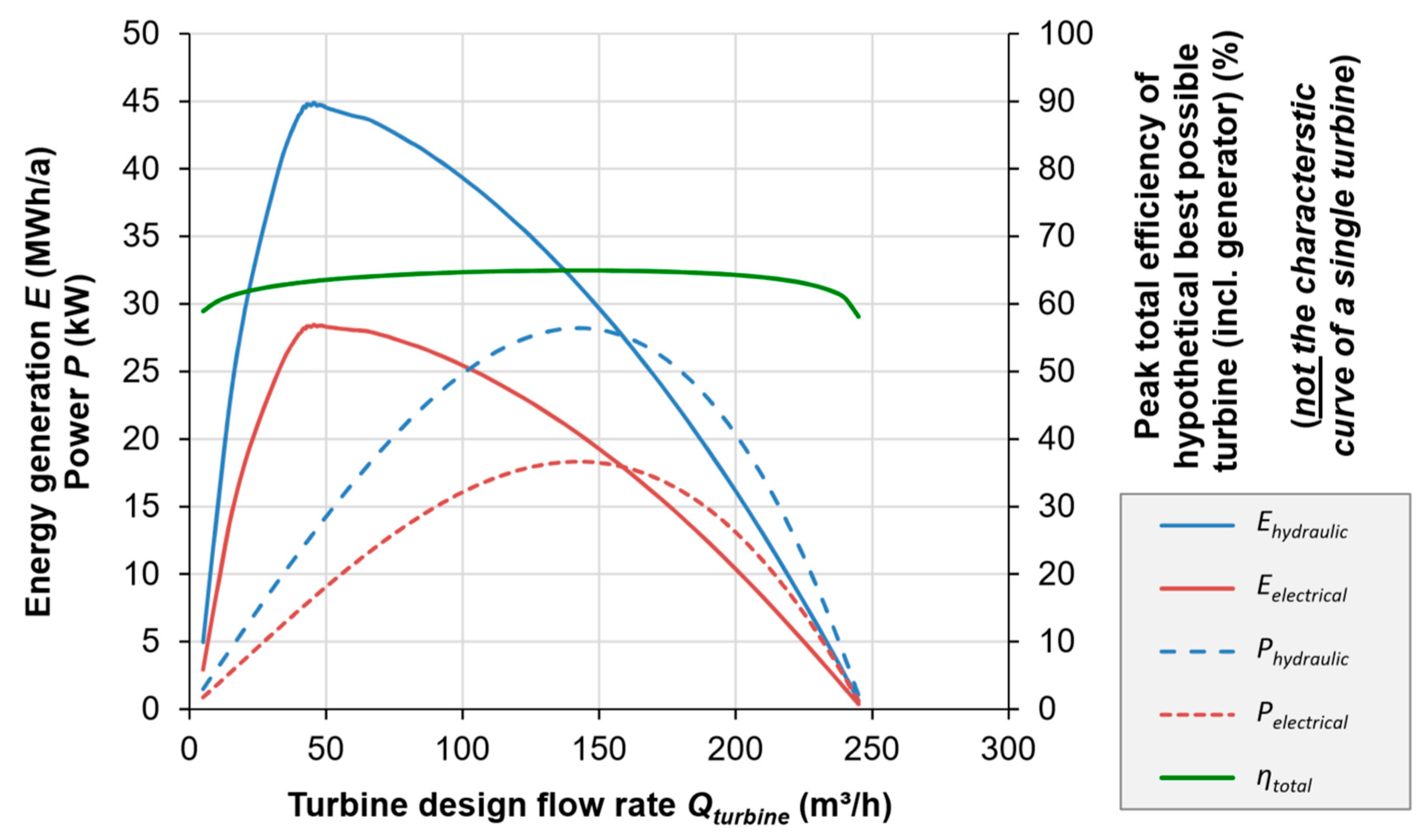
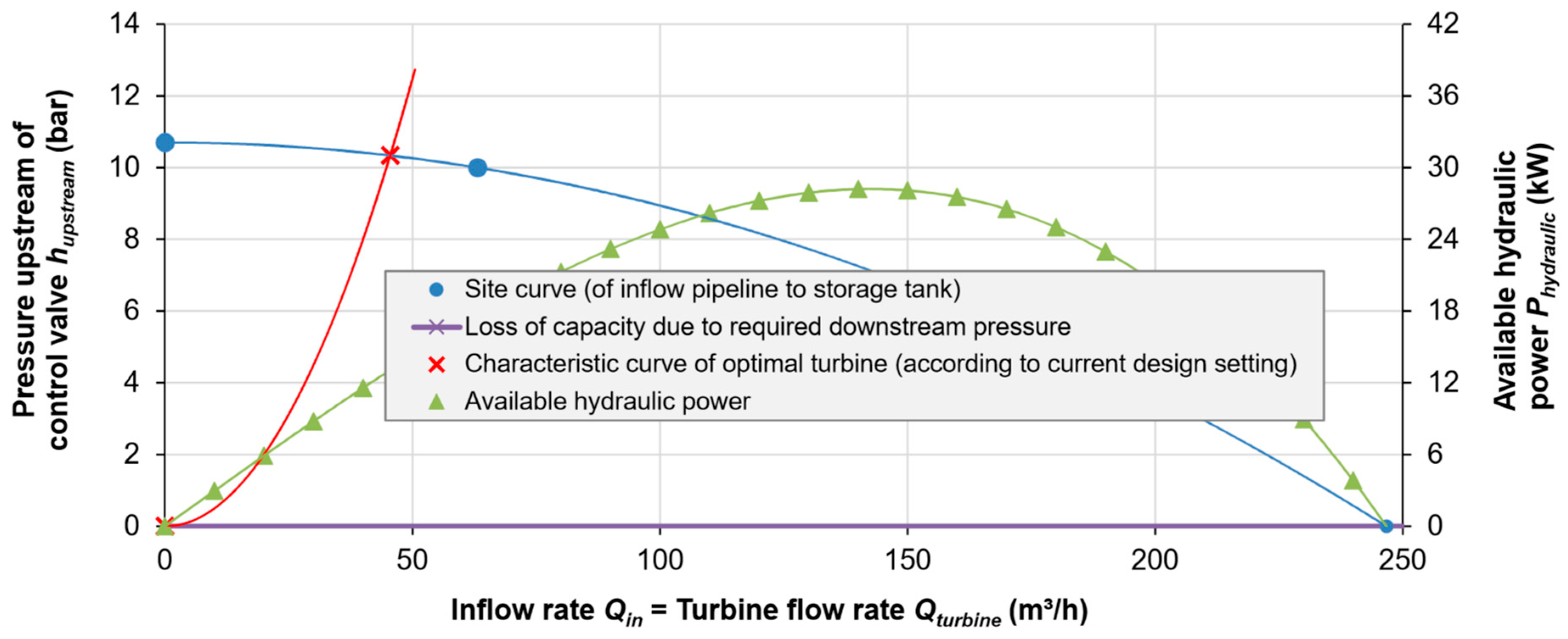
3.1. Case Study of Tool Application: Break Pressure Tank (BPT) Rützengrün, Germany

The best way to understand the methodology implemented in the tool is to follow its use step-by-step for a real-world example and show the data and results as they appear to the user. A blank version of the tool as well as a version with the data for the example site BPT Rützengrün is included in the Supplementary Materials. BPT Rützengrün of the water supply utility ZWAV Plauen is located above the city of Auerbach in the Vogtland region of Saxony and receives its water (via the higher elevation BPT Vogelsgrün) from the long-range water supplier Südsachsen Wasser out of the drinking water reservoir Carlsfeld, located about 180 m above. Figure 5 shows a diagram of this supply system. The BPT serves primarily as a pressure-reducing installation, but also has a small storage tank with a capacity of about 100 m³. Thanks to this storage, BPT Rützengrün is a class 1 site, which permits a degree of flexibility in regulating the inflow and turbine flow rate.

Figure 6 shows the first input mask, in which the user enters the minimum required information in the form of single values. Depending on the choice of calculation option (in this case option 1 and 2), those cells requiring user input turn orange. To determine the most reliable turbine parameters, the planner must not only supply the data needed to define the site curve, but also provide information about the storage tank, including volume and the feasible tank level thresholds for opening and closing the inflow valve. As per the recommended setting, the bypass flow rate Q_bypass is set equal to the maximum permissible inflow rate, in this case 90 m³/h.

The second input mask (not shown here) is for the time series. For BPT Rützengrün, the input time series of Q_out from the tank (to the downstream supply zones) ranged from 29.05.2017 to 15.02.2018 and was processed from so-called delta-event (event-based recording) raw data to have a 15-min time interval. These data are necessary to achieve reliable results. While historical time series for water level and tank inflow rate can be used by the tool to infer the storage tank volume (hence the input fields), they were neither available nor necessary, since the volume was known to be 100 m³. With the information about tank volume and the switching thresholds provided in the first input mask (Figure 6), the tank operation was simulated to determine both acceptable and optimal turbine parameters. This “simulation” consists of a simple numerical model (see Section 2.5), modifying a starting value for the tank level according to the net change in storage volume, as calculated by the difference between the inflow and outflow volumes. The planner must also choose between two types of turbines. In this case, the in-line AXENT turbine was chosen (see Section 2.7 for more details).

Once all necessary input data has been provided, the Visual Basic (VBA) algorithms are run to determine the optimal turbine parameters under the given boundary conditions. The algorithms iteratively progress through all possible design flow rates (see Section 2.5 through Section 2.8), computing and graphically plotting the corresponding performance parameters annual energy generation (E_hydraulic as well as E_electrical), power (P_hydraulic and P_electrical) and total efficiency η_total for the chosen turbine type at the corresponding P_hydraulic (for the best possible turbine, not the characteristic curve of a single turbine—see Section 2.7) (Figure 7). The optimal parameters (head and flow rate) are also displayed and added to the site curve diagram (Figure 8).

After determining the optimal turbine parameters, the annual financial benefits B_annual are determined based on the information provided. In the same step, the total costs for purchase and installation of the turbine C_total are calculated on the basis of available values from the authors’ experience, to roughly estimate the simple (non-inflation-adjusted) payback period (see Section 2.9 for more information). In the case of BPT Rützengrün for the input data shown here and using the recommended calculation and bypass options, E_electrical is estimated at 26,000 kWh/a (

Table 4. Summary of the results for BPT Rützengrün using all four methods described in this article.

	Method	(1) HTWD 2018	(2) DVGW 1994	(3i) DVGW 2016, a 1	(3ii) DVGW 2016, a 2	(4) DVGW 2016, b
Parameter
Flow rate Qturbine (m3/h)		41.0	142	12.5		63.1
Pressure drop hturbine (m)		106	72.7	109		102
Hydraulic power Phydraulic (kW)		11.8	28.2	3.7		17.5
Annual energy generation Eelectrical, nominal (kWh/a)		26,000	18,500	13,700	5300	25,600
Annual electrical energy generation Eelectrical, corrected for flow volume (kWh/a) 3		45,700	32,500	24,000	9300	44,800
Annual electrical energy generation Eelectrical, corrected (% of result via HTWD method)		100%	71.2%	52.7%	20.4%	98.3%

¹ Method applied improperly, as if class 1 site (see Section 2.10 for elaboration); ² method applied properly, as if class 2 site; ³ increased by a factor of 1.75 to account for expected future flow volumes (see Figure 9 and preceding discussion).

) and the payback period at 10.0 years. According to the water supply company ZWAV Plauen, if the turbine lifetime can be assumed at 20 years, the payback period must be ≤ 10 years (less than half of the device’s lifetime) to be an acceptable investment. A turbine at this site would therefore be borderline economically viable according to this assessment.

3.2. Assessing the Impact of Quality Control for Input Data

This case study also provides an opportunity to show the importance of critically assessing the data used. Figure 9 shows the time series of outflow data for BPT Rützengrün. It is clear upon inspection that the period of available data at sufficient resolution (at 15-min rather than 2-h intervals) and without gaps (which cause errors in the calculation) was not representative of the typical past operation and the expected typical future operation of BPT Rützengrün. While these data were sufficient for determining the optimal turbine parameters using the Excel tool, they estimated a much lower annual flow volume V_annual (144,000 m³/a) than was normal in the past and is expected for future operation (252,000 m³/a), based partially on the multi-year 2-h data. This was corroborated by the ZWAV Plauen staff, who explained that the period captured as 15-min values was unusual due to some maintenance work that was performed on the supply system. To compensate for this, E_electrical and consequently B_annual were linearly increased by multiplication with the ratio between these flow volumes, a factor of 1.75. This adjustment increases E_electrical from 26,000 to 45,600 kWh/a and lowers the payback period from 10.0 to 5.7 years (Table 4), making this project much more economically attractive than would have been the case without a careful analysis of the data. This highlights the fact that the acquisition and handling of data is not always straightforward, and ought to be done with a critical eye.

Experience with this site also demonstrated the importance of sufficiently high temporal resolution for the input data. Due to the low storage volume of 100 m³, a time interval greater than 15 min led to an unreliable simulation of the tank levels, since the incremental change in storage volume at times exceeded the tank capacity. In this case, only 2-h values were available for a longer time period (Figure 9). As these occasionally exceeded 50 m³/h, more than 100 m³ would potentially leave the tank in a single time interval. This allows no opportunity for the simulation to react by opening the inflow valve in response to the tank level falling below the switching threshold—the tank would simply be “instantly” emptied. This led the authors to embrace a rule of thumb that 15 min ought to be the maximum time interval between values for Q_out, even if not always strictly necessary, such as for sites with more than 1000 m³ of storage. In general, a longer input time series is better than a shorter one, but as mentioned in Section 2.8 and for reasons made clear here, there is a trade-off between having a sufficiently long dataset for capturing the seasonally varying conditions and accidentally capturing conditions that are obsolete or unlikely to be representative of the future. A period of 12 to 24 months should be sufficient in most cases, but should also be checked for anomalies.

Some other authors have used long-term average values in their turbine design methods [15,25]. It is worth noting that average hourly or average daily flow data can be misleading, since the inflow rate might be much higher than the hourly average but occurring only periodically for only short periods of time (e.g., for 5 min at a time, with 15 min in between times of active flow). If this were to persist for 60 min, the hourly average flow rate would be four times lower than the actual flow rate when the inflow valve is opened, since the water volume would have flowed over 15 min rather than 60 min. The authors have encountered this situation multiple times. Designing a turbine based on the average hourly flow rate without planning to adjust the inflow rate can therefore lead to a large error, since the actual flow rate greatly deviates from the inferred flow rate based on average hourly data.

3.3. Comparison of Results Using the Newly Proposed Method with Other Methods

One purpose of this article is to compare the newly introduced method with existing methods for determining turbine parameters. Figure 10 illustrates application of method “a” suggested by the 2016 DVGW guidelines (Table 3), based on selecting the inflow rate (Q_out) range with the highest estimated energy generation. In this case, the Q_out range from 10 to 15 m³/h is both the most frequent and most promising for highest energy generation. Thus, an average flow rate of 12.5 m³/h emerges as the design flow rate Q_turbine. It is worth noting that the frequency of occurrence of a range of flow rates does not imply that this range will have the greatest estimated energy generation, due to the other factors that influence energy generation, such as the efficiency of the expected turbine (which declines rapidly with declining power rating), occasionally high demand that reduces energy generation at lower design flow rates (due to the necessity of bypassing more water around the turbine) and the increase in frictional head losses (with increasing flow rate). For example, the flow rate ranges 25 to 30 m³/h and 30 to 35 m³/h have nearly the same frequency, but the latter range has a substantially greater expected annual energy generation.

The 1994 DVGW guidelines suggest that the point of maximum hydraulic power P_hydraulic is also the optimal operating point for a turbine (Table 3). This point can be seen on the green curve of Figure 11, corresponding to a P_hydraulic of 28.2 kW and occurring at a flow rate of 142 m³/h. A hypothetical turbine suitable for operating at this point would have a pressure drop h_turbine of 72.7 m, as can be seen where the fictive characteristic curve (red curve with triangle markers) of such a turbine crosses the characteristic site curve of the inflow pipeline for BPT Rützengrün.

Figure 11 also shows the results of the other three methods and their respective hypothetical turbine curves. The green and lavender curves with open circle markers respectively show the P_hydraulic and E_electrical corresponding to each of the turbine operating points. For the 2016 DVGW method “b” (based on inflow rate Q_in), no time series was available, so the single data point used to define the characteristic site curve of the inflow pipeline was taken as the most frequent inflow rate with the highest expected annual energy generation. The corresponding numbers are also summarized in Table 4. The results confirm that the 2018 University of Applied Sciences Dresden (HTWD) method yields the greatest energy generation.

It is important to reiterate (see Section 2.10) that the 2016 DVGW guidelines are explicitly intended for class 2 “non-buffered” sites, in which the system operator can “make the best” out of a hydraulic situation over which they can exercise no control. In this case, the emerging design flow rate of 12.5 m³/h is intentionally “improperly” entered into the HTWD Excel tool, which is built for class 1 “buffered” sites, and modifies the inflow regime to optimize the energy generation. In this way, the only permitted values for Q_in are Q_turbine and Q_bypass—no other inflow rates occur. When properly applied to class 2 sites, this method yields a much lower expected energy generation, since water arriving at all flow rates not falling within a narrow range (e.g., 10 to 15 m³/h) would be bypassed around the turbine. The energy generation possible within other flow rate ranges (represented by the orange columns in Figure 10) would be lost. Using the HTWD tool for a class 1 site, these other orange columns can be almost entirely and efficiently captured by modifying the inflow rate, which is made possible by the storage tank that decouples the inflow and outflow to and from the site. This is the fundamental advantage of a class 1 site.

This difference between the improper and proper application of this method is shown in Table 4 (method 3i vs. 3ii), and highlights the great advantage that class 1 sites have over class 2 sites for energy generation using microturbines with narrow acceptable operating ranges (see Section 2.10 for elaboration). BPT Rützengrün as a class 1 site would have an annual electrical energy generation of about 24,000 kWh/a at the turbine flow rate of 12.5 m³/h, while it would have only 9300 kWh/a if it lacked the 100 m³ storage tank and was therefore a class 2 site—a factor of 2.6 less energy generation.

Furthermore, the use of the 2016 DVGW method “b” (based on the most frequent inflow rate with the highest expected annual energy generation) is also an improper application, since the inflow and outflow at class 2 sites are necessarily equal, as there is no storage tank. However, both of these “improper” applications of the 2016 DVGW method serve as useful comparisons, since in the absence of another method, the designer of a turbine system might choose to select a design flow rate corresponding to a known quantity about the system. As such, this flow rate also generally corresponds to the current operating state, providing a comparison with a design approach that would choose a turbine to fit the existing inflow rate. And as is evident from Table 4, using the substantially higher flow rate of 63.1 m³/h yields a total energy generation that is 98.3% of that yielded by the 2018 HTWD method—in this case hardly a significant loss. However, it cannot be assumed that this will hold true in every case, as the analysis of further sites in the following section shows. In cases where it does hold true, this method can be used to confirm this truth, which provides the designer and operator with a greater level of confidence in the ultimate design decision.

3.4. Results for Nine Sites in Germany

The four turbine design methods were applied to a total of nine sites from Saxony, Germany. The sites had a variety of characteristics and data availability and led to a range of results with varying degrees of confidence (

Table 5. Summary of the site characteristics, with selected design results obtained using the 2018 HTWD method.

Site	Vtank (m3)	Vannual (m3/a)	Qin and havailable before Turbine (Typical Operating Point)	Qin and hturbine with Turbine	Pelectrical (kW)	Qbypass (m3/h)	Confidence in Results
Adorf-Sorge	1000	328,000	145 m3/h 117 m	84 m3/h 139 m	20.7	150	High
Rützengrün	100	252,000 1	63.1 m3/h 102 m	41.0 m3/h 106 m	7.5	90	High
Vogelsgrün	100	158,000	58.3 m3/h 71.3 m	43.5 m3/h 74.9 m	5.6	90	High
Voigtsgrün	4000	255,000	58.8 m3/h 45.3 m	39 m3/h 47.6 m	3.1	100	High
Chursdorf	4000	220,000	24 m3/h 98.3 m	32.5 m3/h 97.6 m	5.4	65	High
Mittweida	1500	260,000	55 m3/h 19.6 m	34 m3/h 21.8 m	2.0	150	Med.
Rochlitz	5000	207,000	61 m3/h 63.2 m	37.5 m3/h 68.9 m	4.4	72	Low
Neundorf	4000	292,000	100 m3/h 39.5 m	50 m3/h 40.4 m	3.4	130	High
Rehbocksberg	10,000	1,800,000	N.A. (new site)	300 m3/h 55.7 m	30.0	360	High

¹ Corrected based on long-term data (see Figure 9 and preceding discussion).

). To highlight the hydraulic differences between the sites, Figure 12 shows the characteristic sites curves of each inflow pipeline—a kind of “finger print” for each site. The current inflow rates range from 24 to 145 m³/h, whereas the newly proposed design flow rates range from 34 to 84 m³/h, with an outlier of 300 m³/h at the newly planned site Rehbocksberg. With the exception of two sites having very small (100 m³) tanks and one site having a very large (10,000 m³) tank, the storage capacity ranged from 1000 to 5000 m³.

For five of the nine sites it was possible to obtain sufficiently detailed data to perform the highest-quality design. In the case of Mittweida, 15-min data existed, but were saved in such a way in the (early generation) SCADA system that made them very time-consuming to retrieve. Thus one-day data were used, which were more easily accessible. For the remaining three sites no time series were available, due to one site not yet existing (the Rehbocksberg storage tank is being newly constructed) and having no SCADA data transmission. The calculation options 3 and 4 in the Excel tool are designed to handle precisely such cases, but the results are to be used with caution.

For Neundorf and Rehbocksberg, the design was based on the operating conditions planned by the respective water utilities, who were confident that they would able to maintain the design turbine flow rates. For Rochlitz, the maximum daily flow volume for any given future year was estimated and used to calculate the corresponding flow rate. This was done by first calculating the average daily flow volume in the month with the greatest flow volume (these data were available), which was 674 m³/d. This number was then multiplied with the ratio (taken from the nearby site Chursdorf) between the maximum daily flow volume in the year and the average daily flow volume in the month with the greatest flow volume, which was 1.34. The resulting “worst-case day” had a flow volume of 900 m³/d, which was assumed to enter the tank over a 24-h period, producing an inflow and turbine design flow rate of 37.5 m³/h.

Table 6. Comparison of the estimated E_electrical (in kWh/a) achieved by four different turbine design methods, in italics as percentages of the value given by method 1.

Site	(1) HTWD 2018 (New Method)			(2) DVGW 1994 kWh/a	(3) DVGW 2016, a kWh/a	(4) DVGW 2016, b kWh/a
	Data Basis: Start Date (Nr. of Days)	Calculation and Bypass Options Used	kWh/a
Adorf-Sorge	27 April 2017 (179)	Calc. 2 Bypass 2	80,900	59,100	78,200	69,800
			100%	73%	97%	86%
Rützengrün	29 May 2018 (256)	Calc. 2 Bypass 2	45,700	32,500	24,100	44,800
			100%	71%	53%	98%
Vogelsgrün	29 May 2018 (256)	Calc. 2 Bypass 2	20,000	14,600	19,500	19,100
			100%	73%	98%	96%
Voigtsgrün	27 April 2017 (179)	Calc. 2 Bypass 2	20,300	14,400	11,000	19,100
			100%	71%	54%	94%
Chursdorf	28 October 2017 (338)	Calc. 2 Bypass 2	36,700	23,300	32,900	29,100
			100%	63%	90%	79%
Mittweida	20 July 2013 (1714)	Calc. 3 Bypass 2	8980	6610	No data	7450
			100%	74%		83%
Rochlitz	Single values, estimates 1	Calc. 4	24,100	17,200	No data	22,400
			100%	72%		93%
Neundorf	Single values, future plans	Calc. 4	19,800	14,000	No data	19,800 100%
			100%	71%
Rehbocksberg	Single values, future plans	Calc. 4	180,000	126,000	No data—new storage tank
			100%	70%
Arithmetic mean	---	---	48,500 100%	34,000 70%	36,500 86%	28,900 91%
Weighted mean	---	---	48,500 100%	34,200 71%	33,100 78%	28,800 91%

¹ Based on the estimated maximum daily flow volume in any given year (see preceding text for clarification).

and

Table 7. Comparison of the estimated annual revenue (in €/a) and simple payback period (in a) for the turbine parameters determined using the four different turbine design methods.

Site	(1) HTWD 2018	(2) DVGW 1994	(3) DVGW 2016, a	(4) DVGW 2016, b
Adorf-Sorge	9980 €/a	7280 €/a	9650 €/a	8600 €/a
	3.6 a	5.1 a	3.8 a	4.3 a
Rützengrün	5630 €/a	4010 €/a	2970 €/a	5530 €/a
	5.7 a	8.8 a	9.6 a	6.1 a
Vogelsgrün	2470 €/a	1800 €/a	2410 €/a	2360 €/a
	12.7 a	18.4 a	12.9 a	13.7 a
Voigtsgrün	2510 €/a	1780 €/a	1350 €/a	2360 €/a
	11.8 a	17.9 a	20.7 a	13.2 a
Chursdorf	4520 €/a	2870 €/a	4060 €/a	3590 €/a
	6.9 a	12.3 a	7.9 a	8.4 a
Mittweida	1110 €/a	815 €/a	No data	919 €/a
	24.2 a	34.8 a		30.7 a
Rochlitz	2980 €/a	2130 €/a	No data	2770 €/a
	10.3 a	15.3 a		11.5 a
Neundorf	2450 €/a	1720 €/a	No data	2450 13.1 a
	12.2 a	20.3 a
Rehbocksberg	22,200 €/a	15,500 €/a	No data—new storage tank
	1.7 a	2.8 a
Arithmetic mean	5980 €/a 9.9 a	4120 €a 15.1 a	4090 €/a 11.0 a	3570 €/a 12.6 a
Weighted mean	3200 €/a 5.3 a	2300€a 8.2 a	2850 €/a 7.6 a	2540 €/a 9.0 a

show a comparison of the technical and economic results, respectively, for all nine sites across all four methods. The HTWD method provides the greatest energy generation for every site. Using the 1994 DVGW method, the energy generation is consistently low, on average only about 71% of the optimum, ranging from 63% to 74%. The 2016 DVGW method “a” (based on the most frequent Q_out with the highest expected annual energy generation) produced very mixed results, ranging from 53% to 98% of the optimum, with a weighted average of 78%. The 2016 DVGW method “b” (based on Q_in) performed consistently better, ranging from 79% to 100% of the optimum and having a weighted average of 91%.

The economic results mirror the technical results. The revenue for all sites was calculated assuming 100% feeding in of the generated electricity, at the 2018 German rate of 12.33 ct. €/kWh, as all sites are eligible for the feed-in tariff under the German Renewable Energy Law. The estimated specific project costs follow a power law and ranged from 1700 €/kW_hydraulic for the highest-capacity turbine (30.0 kW_electrical, Rehbocksberg) to 12,000 €/kW_hydraulic for the lowest-capacity turbine (2.0 kW_electrical, Mittweida), based on past project experience from other sites with similar conditions. The estimated total project costs therefore ranged from approx. 28,000 € to 37,000 €. For the optimal case using the 2018 HTWD method, the annual revenue ranges from 1110 to 22,200 €/a, with simple payback periods from 24.2 to 1.7 years. Of the nine sites, four have payback periods less than 10 years, making them economically viable according to the standards used by the water utility ZWAV Plauen. For the remaining sites, the project costs would have to be reduced in some way to make the installation of a turbine economically viable, for example by reducing the costs of the turbine or other items (see Table 2), or acquiring financial support through state or federal grant funding for renewable energy projects.

4. Discussion

4.1. Archetypical Sites: Handling in Excel Tool and Practical Considerations

During analysis of the nine sites presented here there were five archetypes that emerged, the closer examination of which may prove useful to the reader.

The first archetype is a typical supply tank site, with moderate storage and a more or less typical water demand pattern, reflecting a mixture of household and commercial or industrial users. Voigtsgrün, Chursdorf, Mittweida, Rochlitz, Neundorf and Rehbocksberg fall into this category.

The second archetype is a site that predominantly serves as a break pressure tank along a long-distance pipeline through mountainous terrain. Rützengrün and Vogelsgrün fall into this category. For these two sites in particular, only very small storage tanks (100 m³) are present, which demands that temporally high-resolution outflow data is available to the Excel tool for determining both acceptable and optimal turbine flow rates. As with these two sites (see Figure 5), these kinds of sites can exist in several stages in series, which can have a simplifying cascade effect, since the downstream BPT regulates the outflow of the upstream BPT.

The third archetype is a site with a very flat characteristic site curve, resulting from very low friction losses within the desired operating range of flow rates. Normally this is a consequence of a particularly large inflow pipeline. The sites Rehbocksberg and Neundorf fall into this category (see Figure 12). In this case, the designer has much greater flexibility, because the flow rate can be made higher without risking unnecessary energy loss to pipe wall friction. For example, while the site operator ZWAV Plauen chose 50 m³/h as the design flow rate for Neundorf, a flow rate of 100 m³/h or even 150 m³/h would subtract very little from the total possible energy generation. Both these sites also have high storage capacities of 5000 and 10,000 m³ (although this is not necessarily a property of this archetype), which makes it unlikely that brief periods of high demand would endanger the security of supply by depleting tank levels. Thus, there is also less urgency for having a high-resolution time series of outflow data to verify that the chosen turbine is suitable.

The fourth archetype is a data-lean site, for which only limited information is available. If storage is large enough compared to the demand and the site can be flexibly operated due to system-level redundance (as with Neundorf and Rehbocksberg, which both have parallel supply systems that can replace or supplement water in case of an outage), the limited data may be sufficient to produce a reliable design using the Excel tool. For cases like Rochlitz, however, more data must be gathered to see how the possible short-term spikes in demand impact the energy generation.

The fifth archetype is a site at which energy generation potential may exist, but no economically viable options are available for using the generated electricity. In the case of Adorf-Sorge, which is the second-most promising site after Rehbocksberg, the electrical power output of the turbine at the optimal operating point would be approximately 21 kW. However, the site is located deep in a forest, and is connected to the electricity grid via a 3-km-long cable, such that the maximum possible feed-in power input would be about 2.3 kW before the cable would be overloaded. This low P_electrical could not be economically fed into the grid. There is also not sufficient energy demand at the site (no pumps or other substantial energy users), such that there is currently no known practical way to use the energy that could be generated with a turbine. Unfortunately, this removes Adorf-Sorge from the list of potential sites.

4.2. Cases in Which the Excel Tool is Not Needed or Appropriate

Pragmatic readers may ask themselves whether the data acquisition and evaluation required for using the full functionality of the Excel tool is warranted in every case. There are two main cases in which the designer of a turbine site should elect not to use the tool as recommended:

• There is limited data available for the site and time or other constraints make it undesirable to perform new measurements. In this case the site operator can take the shortcut of using the equivalent of the 2016 DVGW method “b”, and simply select a turbine that operates efficiently at the current typical Q_in. According to the seven sites analyzed here, this leads on average to 10% less energy generation (and annual revenue), with a risk of up to 20% less energy generation. This is the best known alternative method that removes the need for data-based work.
• The site in question is a class 2 “non-buffered” site, for which this tool is not appropriate. Using the tool for class 2 sites will lead to gross overestimates of the potential energy generation, as shown in Table 4. This is due to the fact that the tool assumes a complete modification of the Q_in regime, which is not possible at a class 2 site, for which Q_in is necessarily equal to Q_out.

4.3. Limitations of the Tool

The main limitation of the Excel tool presented here is its lack of functionality for accommodating class 2 “non-buffered” sites without storage tanks. While the authors suspect that class 2 sites with economically viable energy generation potential are in the minority compared to class 1 sites, the authors already identified several sites for which a practical and technically accessible design method would be needed. Collaborators of the authors in 2013 developed a preliminary Excel tool according to this method (currently available only in German [38]), which systematically tests the historical distribution of flow rates against typical efficiency curves for different types of turbines (e.g., Francis, Pelton, pump-as-turbine) to determine both the optimal turbine type and parameters for a given site. However, the authors are not confident that this tool properly accounts for the hydraulic nature of class 2 sites. Future work could pick up where this preliminary tool left off, and perhaps incorporate its functionality directly into the Excel tool presented here. In the best case, this could also build and improve on the 2016 DVGW methods.

The remaining limitations deal with ways in which the methodology and Excel tool might not lead to optimal solutions for class 1 sites, and could be improved in the future:

• The tool assumes the selection of a single turbine with a narrow acceptable operating range, and considers neither the possibility of turbines with wide operating ranges nor that of multiple turbines, the latter of which might lead to greater energy generation [25,27]. This was decided partly for simplicity’s sake and partly out of the belief that a single turbine generally represents the most economically viable solution for class 1 sites, which is supported by one of the studies cited above [25]. Furthermore, as indicated in Section 1.2, these studies do take into account the fundamental advantage of class 1 sites, which is the ability to modify the inflow regime, instead using multiple turbines to adapt to the wide range of flow rates occurring based on the current site conditions.
• The tool does not have a sophisticated way to support users with sites for which a feed-in tariff is either not available or not applicable (e.g., in Germany, if the water does not flow 100% via natural gradient). There is an option to enter in the total energy use on site and the percentage of which the user expects to be covered by the turbine. In the future it is planned to implement an algorithm that takes as input a time series of electricity use on site (parallel to the Q_out time series) and estimates how much of this energy use could be covered by the turbine, such that the user does not need to estimate this herself.
• There is a lack of decision support in accounting for future changes in water use patterns, which other design methods seem to have accounted for [14,39,40]. However, there is a simplified factor which can be adjusted to account for possible increases or decreases in water use. In this way, an expected future water use pattern can be roughly simulated, and a turbine designed that will still be suitable for this future condition.
• The impact of iteratively varying the threshold tank levels (see Figure 6) to activate and deactivate the turbine and bypass has not been sufficiently assessed. Sitzenfrei and Rauch [14] presented an optimization method that is similar in spirit to the one presented by the authors but applied it to a class 2 site. They pursued an optimization approach by varying parameters in a randomized fashion through 1000 simulations (Monte Carlo simulation), selecting the best solution based on the amount of energy generated over 10 years. The parameters varied in this case are the set-point water levels in the supply tank upstream of the turbine: the overflow level, the level for switching from high to low turbine flow, and the minimum level required for fire-fighting. The HTWD method introduced in this paper could be improved by implementing a similar kind of randomized (e.g., Monte Carlo) variation of the four water level thresholds used to determine when water flows through the turbine, bypass or neither. This might increase the robustness of the solution suggested by the tool and also slightly increase the total annual energy generation predicted by the tool.
• As mentioned in Section 3.2, gaps (i.e., time intervals larger than the smallest time interval; e.g., due to missing data) in the input data time series of Q_out lead to an error in the calculations performed by the tool. Currently, the burden is on the user to ensure that the time series contains no gaps. In the future, this could be improved through an algorithm that automatically checks for and linearly interpolates to fill these gaps.
• Currently, the data from only two types of turbines from two manufacturers are incorporated into the tool. This merely reflects the authors’ experience and available data until now and is not intended to imply that there are not further options. No funding links or other conflicts of interest exist between the authors and these two turbine manufacturers.

4.4. Relative Potential of Class 1 vs. Class 2 Sites

As mentioned previously, class 2 sites represent a greater technical challenge for the optimization-minded engineer than class 1 sites. Although they have not been able to confirm it, the authors suspect that class 1 sites exist in greater numbers and possess greater potential for energy generation than class 2 sites, due to their generally higher pressure heads. In particular, class 1 sites seem most relevant for small and medium-sized water suppliers with low population densities and relatively low water distribution flow rates, since their class 2 sites are unlikely to provide economically viable energy generation. It may be the case for the largest water suppliers that class 1 sites were long ago tapped for their hydropower potential, leaving predominantly class 2 sites that remain to be developed. As the largest water suppliers also tend to be more innovative, this may explain the apparently greater scientific attention given to class 2 sites (Appendix A.4). If the authors’ suspicions are accurate, it would be useful to better understand the relative potential for drinking water hydropower at class 1 vs. class 2 sites, as this could provide an incentive for greater focus on supporting the design and development of class 1 sites for small and medium-sized water suppliers, which tend to make up the vast majority in the total count of a given country’s water suppliers. The German water suppliers featured in this study are medium-sized.

5. Conclusions

This paper presented a novel method and accompanying Excel tool for determining the optimal parameters of a microturbine for water supply sites having a storage tank that decouples the inflow and outflow patterns, the so-called class 1 “buffered” sites. The method determines the optimal turbine flow rate based on key site characteristics and a historical time series of outflow data from the tank, simulating tank operation with a numerical model as it creates a new inflow regime. The main criterion for a viable solution is that the tank water level does not fall below a user-specified minimum. The Excel tool is not currently suitable for analyzing class 2 “non-buffered” sites without a storage tank but could conceivably be expanded to include this functionality.

The method was inspired by Haakh [28], who provided a foundational treatment of turbine and pump operation in the context of water supply systems. It fills a gap in the known methods for designing microturbines for water supply sites, which recognize the design advantages of class 1 sites, but provide no practical instructions on how to determine the optimal flow rate and corresponding pressure drop. The tool is intended to be widely accessible by being implemented in the commonly used software Microsoft Excel and is offered free of cost for download and use by any interested parties [33]. A blank version of the tool as well as a version with the data for the example site BPT Rützengrün (see Section 3.1) is included in the supplementary material.

The 2018 HTWD method presented here is compared with three other methods from two different generations of DVGW guidelines from 1994 and 2016. All four methods were used to analyze a total of nine sites located in Saxony, Germany, and the results were compared in terms of the annual energy generation. The HTWD design method estimates the greatest energy generation for each site, whereas the other three methods lead to an average of 70% to 91% of the HTWD results. If an alternative method had to be chosen, the 2016 DVGW method “b” (based on the most frequent range of inflow rates with the highest expected annual energy generation) provided the second-best results overall, ranging from 79% to 100% (with an average of 91%) of the energy generation predicted using the HTWD method (see Section 3.3 and Section 3.4 for details).

Of the nine sites analyzed, four are very likely economically viable (estimated payback periods of 1.7 to 6.9 years), while four are borderline viable (payback in 10.3 to 12.7 years) and could be made viable with sufficient reduction in project costs to the operator, for example through grant funding. The remaining site (Mittweida) is very unlikely economically viable, with an estimated payback period of 24.2 years. Other factors prevent the second-most promising site (Adorf-Sorge) from being economically viable, since there is no known practical way to transport the generated electricity off site or use it on site. While a turbine has not yet been implemented at any of these nine sites, at the time of submission, the site Rehbocksberg is the furthest along in the planning, and should be installed before the end of 2019, the site Rützengrün is in an advanced planning stage and the site Chursdorf is in an early planning stage. The experience gained from analyzing all nine sites led to the description of five archetypical sites (see Section 4.1 for details), which the reader can use as points of reference when analyzing sites under his or her supervision.

References

1. Hintermann, M. Electricity from Drinking Water Systems: Inventory and Feasibility Study of Drinking Water Hydropower Facilities in Switzerland (In German & French Only); Projektleitung DIANE Klein-Wasserkraftwerke; Bundesamt für Energiewirtschaft: Bern, Switzerland, 1994; p. 65. Available online: http://www.infrawatt.ch/sites/default/files/1994_DIANE_4df_Elektrizit%C3%A4t%20aus%20Trinkwasser-Systemen.pdf (accessed on 1 April 2019).
2. EnergieSchweiz und SVGW. Energy in the Water Supply: Guidebook for Optimizing Energy Costs and Operation (In German Only); Bundesamt für Energie und SVGW: Zurich, Switzerland, 2004. [Google Scholar]
3. Aste, C.M.; Moritz, G. TrinkHYDRO-Kärnten: Assessment of the Potential for Drinking Water Power Plants in Kärnten (In German Only); Technical report nr. B-EBK 9-036; ELWOG: Klagenfurt, Austria, 2009. [Google Scholar]
4. Laghari, J.A.; Mokhlis, H.; Bakar, A.H.A.; Mohammad, H. A comprehensive overview of new designs in the hydraulic, electrical equipments and controllers of mini hydropower plants making it cost effective technology. Renew. Sustain. Energy Rev. 2012, 20, 279–293. [Google Scholar] [CrossRef]
5. McNabola, A.; Coughlan, P.; Corcoran, L.; Power, C.; Williams, A.P.; Harris, I.; Gallagher, J.; Styles, D. Energy recovery in the water industry using micro-hydropower: An opportunity to improve sustainability. Water Policy 2013, 1–16. [Google Scholar] [CrossRef]
6. McNabola, A.; Coughlan, P.; Williams, A.P. Energy recovery in the water industry: An assessment of the potential of micro-hydropower. Water Environ. J. 2013, 1–11. [Google Scholar] [CrossRef]
7. Ramos, H.M.; Mello, M.; De, P.K. Clean power in water supply systems as a sustainable solution: From planning to practical implementation. Water Sci. Technol. Water Supply 2010, 10, 39–49. [Google Scholar] [CrossRef]
8. Carravetta, A.; Fecarotta, O.; Ramos, H.M. A new low-cost installation scheme of PATs for pico-hydropower to recover energy in residential areas. Renew. Energy 2018, 2. [Google Scholar] [CrossRef]
9. Pérez-Sánchez, M.; Sánchez-Romero, F.J.; López-Jiménez, P.A.; Ramos, H.M. PATs selection towards sustainability in irrigation networks: Simulated annealing as a water management tool. Renew. Energy 2017. [Google Scholar] [CrossRef]
10. Corcoran, L.; McNabola, A.; Coughlan, P. Energy Recovery Potential of the Dublin Region Water Supply Network. In Proceedings of the World Congress on Water, Climate and Energy, Dublin, Ireland, 13–18 May 2012. [Google Scholar]
11. Corcoran, L.; Coughlan, P.; McNabola, A. Energy recovery potential using micro hydropower in water supply networks in the UK and Ireland. Water Sci. Technol. Water Supply 2013, 13, 552–560. [Google Scholar] [CrossRef]
12. DVGW. Energy Recovery through Hydropower Facilities in the Water Supply (In German Only); Technical Guidelines, Worksheet W 613 (A); DVGW: Bonn, Germany, 2016. [Google Scholar]
13. Carravetta, A.; Del Giudice, G.; Fecarotta, O.; Ramos, H.M. Energy Production in Water Distribution Networks: A PAT Design Strategy. Water Resour. Manag. 2012, 26, 3947–3959. [Google Scholar] [CrossRef]
14. Sitzenfrei, R.; von Leon, J.; Rauch, W. Design and Optimization of Small Hydropower Systems in Water Distribution Networks Based on 10-Years Simulation with Epanet2. Procedia Eng. 2014, 89, 533–539. [Google Scholar] [CrossRef] [Green Version]
15. Power, C.; Coughlan, P.; McNabola, A. Microhydropower Energy Recovery at Wastewater-Treatment Plants: Turbine Selection and Optimization. J. Energy Eng. 2016. [Google Scholar] [CrossRef]
16. Lima, G.M.; Brentan, B.M.; Luvizotto, E. Optimal design of water supply networks using an energy recovery approach. Renew. Energy 2017. [Google Scholar] [CrossRef]
17. Samora, I.; Manso, P.; Franca, M.J.; Schleiss, A.J.; Ramos, H.M. Feasibility Assessment of Micro-Hydropower for Energy Recovery in the Water Supply Network of the City of Fribourg; Sustainable Hydraulics in the Era of Global, Change; Erpicum, S., Dewals, B., Archambeau, P., Pirotton, M., Eds.; Taylor & Francis Group: London, UK, 2016; pp. 961–965. ISBN 978-1-138-02977-4. [Google Scholar]
18. Samora, I.; Franca, M.J.; Schleiss, A.J.; Ramos, H.M. Simulated Annealing in Optimization of Energy Production in a Water Supply Network. Water Resour. Manag. 2016, 230, 1533–1547. [Google Scholar] [CrossRef]
19. Carravetta, A.; del Guidice, G.; Fecarotta, O.; Ramos, H.M. PAT Design Strategy for Energy Recovery in Water Distribution Networks by Electrical Regulation. Energies 2013, 6, 411–424. [Google Scholar] [CrossRef] [Green Version]
20. Fecarotta, O.; Ramos, H.M.; Derakhshan, S.; Del Giudice, G.; Carravetta, A. Fine Tuning a PAT Hydropower Plant in a Water Supply Network to Improve System Effectiveness. J. Water Resour. Plan. Manag. 2018, 144. [Google Scholar] [CrossRef]
21. Novara, D.; McNabola, A. The Development of a Decision Support Software for the Design of Micro-Hydropower Schemes Utilizing a Pump as Turbine. Proceedings 2018, 2, 678. [Google Scholar] [CrossRef]
22. Pérez-Sánchez, M.; López-Jiménez, P.A.; Ramos, H.M. PATs Operating in Water Networks under Unsteady Flow Conditions: Control Valve Manoeuvre and Overspeed Effect. Water 2018, 10, 29. [Google Scholar] [CrossRef]
23. Vilanova, M.R.N.; Balestieri, J.A.P. Hydropower recovery in water supply systems: Models and case study. Energy Convers. Manag. 2014, 84, 414–426. [Google Scholar] [CrossRef]
24. Novara, D. Energy Harvesting from Municipal Water Management Systems: From Storage and Distribution to Wastewater Treatment. Extended Abstract (Not Peer-Reviewed). 2016. Available online: https://fenix.tecnico.ulisboa.pt/downloadFile/281870113703554/Extended%20Abstract%20-%20Daniele%20Novara.pdf (accessed on 9 January 2019).
25. Monteiro, L.; Delgado, J.; Covas, D.C. Improved Assessment of Energy Recovery Potential in Water Supply Systems with High Demand Variation. Water 2018, 10, 773. [Google Scholar] [CrossRef]
26. Kucukali, S. Water supply lines as a source of small hydropower in Turkey: A Case study in Edremit. In Proceedings of the World Renewable Energy Congress 2011, Hydropower Applications, Linköping, Sweden, 8–13 May 2011; pp. 1400–1407. Available online: http://www.ep.liu.se/ecp/057/vol6/004/ecp57vol6_004.pdf (accessed on 5 March 2019).
27. Kougias, I.; Patsialis, T.; Zafirakou, A.; Theodossiou, N. Exploring the potential of energy recovery using micro hydropower systems in water supply systems. Water Util. J. 2014, 7, 25–33. [Google Scholar]
28. Haakh, F. Hydraulic Aspects of the Economic Viability of Pumps, Turbines and Pipelines in the Water Supply (In German Only), 1st ed.; HUSS-MEDIEN GmbH: Berlin/Oldenbourg, Germany; Industrieverlag: München, Germany, 2009; pp. 111–174. ISBN 978-3410211389. [Google Scholar]
29. Kracht, S. Out of water comes electricity—Microturbine “PAM PERGA” in water supply network (in German only). Energie|Wasser-Praxis 2018, 10, 78–81. [Google Scholar]
30. Wieprecht, S.; Kramer, M. Investigations into the Use of Microturbines in Drinking Water Supply and Distribution Networks; Technical report nr. 09/2012; Funded under DVGW Project W8/01/10; DVGW: Bonn, Germany, 2012. [Google Scholar]
31. Plath, M.; Wichmann, K.; Ludwig, G. Handbook for Energy Efficiency and Energy Savings in the Water Supply (In German Only); DVGW & DBU: Bonn/Osnabrück, Germany, 2010. [Google Scholar]
32. Parra, S.; Krönlein, F.; Krause, S.; Günthert, F.W. Energy generation in the water distribution network through intelligent pressure management (in German only). Energie|Wasser-Praxis 2015, 12, 99–103. [Google Scholar]
33. Voltz, T.; Grischek, T. Energy management in the water supply: Excel Toolbox. Available online: https://www.htw-dresden.de/energy-in-water (accessed on 4 July 2019).
34. DVGW. Energy Recovery through Hydropower Facilities in the Water Supply (In German Only); Technical guidelines, Worksheet W 613; DVGW: Eschborn, Germany, 1994. [Google Scholar]
35. Stellba Hydro: Axent. Available online: http://www.stellba-hydro.com/axent/ (accessed on 13 December 2018).
36. KSB. Application-Oriented Planning Documents for Pumps as Turbines. Available online: https://www.ksb.com/blob/52858/13564c16a6b15b3c28b1d544ae52d0e4/pat-en-data.pdf (accessed on 5 May 2019).
37. Mikus, K. Energy savings and recovery in drinking water supply (in German only). In Mechanical and Electrical Installations in Water Works, 1st ed.; Ebel, O.-G., Ed.; DVGW & Oldenbourg Industrieverlag: München, Germany, 1995; Volume 3, pp. 93–98. ISBN 3-486-26339-0. [Google Scholar]
38. Bahner, P.; Voltz, T.; Grischek, T. Bemessung von Pumpen als Turbinen. Available online: https://www2.htw-dresden.de/~wasser5/ (accessed on 5 July 2019).
39. Corcoran, L.; McNabola, A.; Coughlan, P. Predicting and quantifying the effect of variations in long-term water demand on micro-hydropower energy recovery in water supply networks. Urban Water J. 2016. [Google Scholar] [CrossRef]
40. Colombo, A.; Kleiner, Y. Energy recovery in water distribution systems using microturbines. In Proceedings of the Probabilistic Methodologies in Water and Wastewater Engineering, Toronto, ON, Canada, 23–27 September 2011; pp. 1–9. [Google Scholar]
41. Brown, L. Understanding Gravity-Flow Pipelines. Livestock Watering Factsheet. January 2006. British Columbia Ministry of Agriculture and Lands, Order No. 590.304–5. Available online: https://www.itacanet.org/doc-archive-eng/water/gravity_flow_pipelines.pdf (accessed on 12 December 2018).
42. Chapallaz, J.-M.; Eichenberger, P.; Fischer, G. Manual on Pumps Used as Turbines, MHPG Series, Harnessing Water Power on a Small Scale, 11, GATE, GTZ, Eschborn. 1992. Available online: Skat.ch/book/manual-on-pumps-used-as-turbines-volume-11/ (accessed on 16 March 2019).
43. Chapallaz, J.-M.; Mombelli, H.-P.; Renaud, A. Small Hydropower Plants: Water Turbines (In German Only); Impulsprogramm PACER; Bundesamt für Konjunkturfragen: Bern, Switzerland, 1995; ISBN 3-905232-54-5. [Google Scholar]
44. Jesinger, G. Possibilities and limits of energy recovery in water supply facilities (in German only). In Proceedings of the 11th Technical Water Seminar, Report Nr. 73, Munich, Germany, 22 October 1986; Bischofsberger, W., Ed.; TU Munich: Munich, Germany, 1987; pp. 185–210. [Google Scholar]
45. Heinzmann, K. Experiences with pressure-relieving turbines—Munich water works (in German only). In Proceedings of the 11th Technical Water Seminar, Report Nr. 73, Munich, Germany, 22 October 1986; Bischofsberger, W., Ed.; TU Munich: Munich, Germany, 1987; pp. 211–228. [Google Scholar]
46. Mikus, K. Experiences with pressure-relieving turbines—Stuttgart technical works (in German only). In Proceedings of the 11th Technical Water Seminar, Report Nr. 73, Munich, Germany, 22 October 1986; Bischofsberger, W., Ed.; TU Munich: Munich, Germany, 1987; pp. 237–252. [Google Scholar]
47. Schatz, J. Experiences with pressure-relieving turbines—Long-range water supply of Mühlveirtel/Austria (in German only). In Proceedings of the 11th Technical Water Seminar, Report Nr. 73, Munich, Germany, 22 October 1986; Bischofsberger, W., Ed.; TU Munich: Munich, Germany, 1987; pp. 229–236. [Google Scholar]
48. Williams, A.A.; Smith, N.P.A.; Bird, C.; Howard, M. Pumps as Turbines and the Induction Motors as Generators for Energy Recovery in Water Supply Systems. Water Environ. J. 1998, 12, 175–178. [Google Scholar] [CrossRef]
49. Voltz, T.J.; Bahner, P.; Grischek, T. Energy efficiency of pumps and small turbines—Case studies (in German only). In Proceedings of the 2nd Saxon Drinking Water Conference, Dresden, Germany, 5 September 2013; Grischek, T., Ed.; DVGW: Dresden, Germany, 2013; pp. 99–112. [Google Scholar]
50. Gaius-obaseki, T. Hydropower opportunities in the water industry. Int. J. Environ. Sci. 2010, 1, 392–402. [Google Scholar]
51. Baumann, R.; Juric, T. The counter pressure Pelton turbine as a solution for energy generation in drinking water systems (in German only). Wasserwirtschaft 2010, 7–8, 15–18. [Google Scholar]
52. Bahner, P. Deployment of Microturbines in Drinking Water Supply Networks of the FWV Elbaue-Ostharz GmbH (In German only). Diploma Thesis, Faculty of Civil Engineering, University of Applied Sciences (HTW), Dresden, Germany, 2013. [Google Scholar]
53. De Marchis, M.; Fontanazza, C.M.; Freni, G.; Messineo, A.; Milici, B.; Napoli, E.; Notaro, V.; Puleo, V.; Scopa, A. Energy recovery in water distribution networks. Implementation of pumps as turbine in a dynamic numerical model. Procedia Eng. 2014, 70, 439–448. [Google Scholar] [CrossRef]
54. Fecarotta, O.; McNabola, A. Optimal Location of Pump as Turbines (PATs) in Water Distribution Networks to Recover Energy and Reduce Leakage. Water Resour. Manag. 2017, 31, 5043–5059. [Google Scholar] [CrossRef]
55. Giugni, M.; Fontana, N.; Ranucci, A. Optimal Location of PRVs and Turbines in Water Distribution Systems. J. Water Resour. Plan. Manag. 2014, 140. [Google Scholar] [CrossRef]
56. Lima, G.M.; Luvizotto, E.; Brentan, B.M. Selection and location of pumps as turbines substituting pressure reducing valves. Renew. Energy 2017. [Google Scholar] [CrossRef]
57. Santolin, A.; Cavazinni, G.; Pavesia, G.; Ardizzon, G.; Rossetti, A. Techno-economical method for the capacity sizing of a small hydropower plant. Energy Convers. Manag. 2011, 52, 2533–2541. [Google Scholar] [CrossRef]
Figure 1. Key difference between class 1 (“buffered”) and class 2 (“non-buffered”) sites, based on data from 27 April 2017 from the class 1 site “Voigtsgrün” in Saxony, Germany (the isolated, very high peaks occurring between 00:00 and 04:00 and at 18:00 are due to a beer brewery). *This illustration only intends to show the turbine in parallel to the control valve; the turbine does not need to be located above the control valve and is typically located at nearly the same elevation.
Water 11 01403 g001
Figure 2. Visual explanation of some key parameters used in the method, as introduced in Section 2.2 and Section 2.5. * Note that hmax depends on the current water level in the upstream tank, which is why the measurement of h1_upstream and h2_upstream should be conducted when the upstream tank is known to be at its typical lowest level.
Water 11 01403 g002
Figure 3. Global efficiency data for AXENT and pumps-as-turbines (PAT) microturbines, with best-fit natural log curves.
Water 11 01403 g003
Figure 4. Specific project costs for AXENT and PATs, with best-fit power law curves.
Water 11 01403 g004
Figure 5. Diagram of the Carlsfeld supply system, with break pressure tank (BPT) Vogelsgrün and BPT Rützengrün. As illustrated in Figure 1, the potential turbines would be positioned in parallel with the existing pressure control valves.
Water 11 01403 g005
Figure 6. Excerpt of the first data input mask for single values, with values for BPT Rützengrün.
Water 11 01403 g006
Figure 7. Calculated performance parameters of hypothetical turbines (at best efficiency point) with iteratively varied design flow rates (here from 5 to 245 m3/h), with values for BPT Rützengrün.
Water 11 01403 g007
Figure 8. Site curve of BPT Rützengrün with characteristic curves of the corresponding hydraulic power as well as the (hypothetical) turbine with optimal operating parameters. 1 bar = 10.19 m of head.
Water 11 01403 g008
Figure 9. Outflow data series available for BPT Rützengrün, with the data used in the Excel tool highlighted in orange.
Water 11 01403 g009
Figure 10. Frequency distribution of outflow rates and corresponding estimated annual electrical energy generation per flow rate class, at 15-min intervals for BPT Rützengrün.
Water 11 01403 g010
Figure 11. Site curve of BPT Rützengrün, hypothetical turbine curves for design results of all four methods, and corresponding hydraulic power as well as estimated annual electrical energy generation at each operating point.
Water 11 01403 g011
Figure 12. Overview of the hydraulic characteristic curves for all nine sites analyzed.
Water 11 01403 g012