Impacts of Climate Change and Land-Use Change on Hydrological Extremes in the Jinsha River Basin

Abstract

Hydrological extremes are closely related to extreme hydrological events, which have been and continue to be one of the most important natural hazards causing great damage to lives and properties. As two of the main factors affecting the hydrological cycle, land-use change and climate change have attracted the attention of many researchers in recent years. However, there are few studies that comprehensively consider the impacts of land-use change and climate change on hydrological extremes, and few researchers have made a quantitative distinction between them. Regarding this problem, this study aims to quantitatively distinguish the effects of land-use change and climate change on hydrological extremes during the past half century using the method of scenarios simulation with the soil and water assessment tool (SWAT). Furthermore, the variations of hydrological extremes are forecast under future scenarios by incorporating the downscaled climate simulations from several representative general circulation models (GCMs). Results show that: (1) respectively rising and declining risks of floods and droughts are detected during 1960–2017. The land use changed little during 1980–2015, except for the water body and building land. (2) The SWAT model possesses better simulation effects on high flows compared with low flows. Besides, the downscaled GCM data can simulate the mean values of runoff well, and acceptable simulation effects are achieved for the extreme runoff indicators, with the exception of frequency and durations of floods and extreme low flows. (3) During the period 1970–2017, the land-use change exerts little impact on runoff extremes, while climate change is one of the main factors leading to changes in extreme hydrological situation. (4) In the context of global climate change, the indicators of 3-day max and 3-day min runoff will probably increase in the near future (2021–2050) compared with the historical period (1970–2005). This research helps us to better meet the challenge of probably increased flood risks by providing references to the decision making of prevention and mitigation measures, and thus possesses significant social and economic value.

1. Introduction

In recent years, hydrological responses in a changing environment have become a research hotspot [1,2,3]. As the major factors affecting hydrological processes, land-use change and climate change have been given much attention [4,5,6,7]. Meanwhile, increasingly frequent extreme hydrological events have become an important area of research due to their strong destructive power [8,9,10].

Many scholars have studied hydro-meteorological extremes and a series of important conclusions have been drawn as follows. The hydrological cycle is expected to be intensified in the context of global warming [11,12,13]. Although no obvious trend exists in global averaged precipitation during the instrumentation period [14], some researchers have detected increases in extreme precipitation in most part of the world [15,16,17]. Furthermore, projections from climate models indicate that the precipitation extremes will further increase in the 21st century [18,19,20], which will consequently result in more frequent floods [21], thus posing a threat to water security and bringing challenges to the sustainable development of human society. Regarding land-use change, this is the other critical factor influencing rainfall-runoff processes by affecting surface runoff components, such as evapotranspiration and infiltration. Although there has been a lot of research on the hydrological responses of land-use change in the past few years [22,23,24,25,26], and many researchers have attempted to analyze its impact on runoff extremes at the event scale [27,28,29,30], the relationship between land use and hydrology still remains to be resolved. Therefore, the analysis and prediction of hydrological extremes under land-use change and climate change are of great importance for the prevention and mitigation of hydrological disasters.

Looking through the literature, many scholars have studied the impacts of climate change and land use change on the water availability [31,32,33,34], and plenty of studies have focused on the effects of climate change [35,36,37,38] or land-use change [26,29,39,40,41] on extreme hydrological events. However, few studies exist that take into consideration both the above two factors for the research of extreme hydrology [42], let alone the fact that some of the relating studies concentrate on the probable maximum flood (PMF), which is estimated for the determination of design floods of water conservancy projects [43]. Accordingly, more work is needed to evaluate the effects of land-use change and climate change on hydrological extremes.

The hydrological extremes can be obtained by combining downscaled general circulation models (GCMs) data with a hydrological model [44,45,46]. In this research, the soil and water assessment tool (SWAT) is adopted for runoff simulation, and the daily bias correction (DBC) method is used to downscale the GCM outputs, including precipitation and min/max temperature. The simulation effects of SWAT model and the performance of downscaled GCM data in runoff simulation are respectively evaluated in the paper.

Located at the source of the Yangtze River, the Jinsha River Basin is extremely abundant in hydropower resources. However, the hydrological processes have changed significantly with global climate change and the intensification of anthropogenic activities [47]. The safe and sustainable development of its hydropower resources plays an important role in the promotion of the Western Development Strategy in China. Therefore, it is of great significance to carry out research on hydrological extremes in a changing environment in this basin.

Two objectives are to be achieved in this research. Firstly, quantitatively distinguishing the effects of climate change and land use change on hydrological extremes over the past half century by means of SWAT model. Secondly, predicting the variations and trends of hydrological extremes in the near future by incorporating the bias corrected GCMs projections. To accomplish that, the temporal and spatial analysis of extreme precipitation, temperature and runoff series are conducted during the instrumentation period. A daily scale SWAT model is established in the basin, by means of which scenarios simulations are performed to quantitatively distinguish the extreme hydrological response to climate change and land-use change, with several indicators of hydrologic alteration (IHA) parameters incorporated. Then the hydrological extremes are predicted in the future by combining climate model simulations with the hydrological model.

2. Study Area and Materials

2.1. Study Area

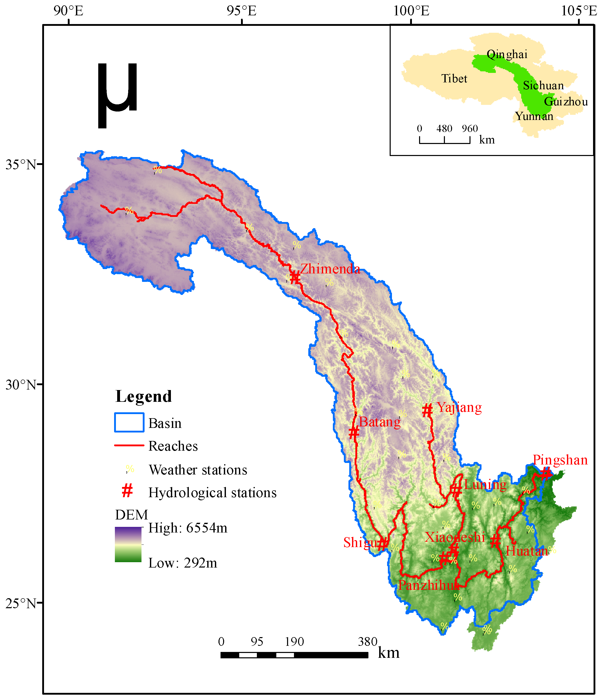
As the source of the Yangtze River, the Jinsha River originates from the Tanggula Mountain on the Eastern Tibetan Plateau and flows through the Hengduan Mountainous region and the Yunnan-Guizhou Plateau (Figure 1). The Jinsha River Basin possesses a vast drainage area of 45.5 × 10⁴ km², spanning five administrative provinces of Qinghai, Tibet, Sichuan, Yunnan and Guizhou. The Yalong River, on which the Yajiang, Luning and Xiaodeshi hydrological stations are located, is the largest tributary of the Jinsha River. It flows from Qinghai into Sichuan province and merges into the Jinsha River in Panzhihua City.

The Jinsha River Basin is characterized by the extremely complicated topography, with the elevation differences over 6000 m, making it extraordinarily rich in hydropower resources. The annual average precipitation, discharge and temperature in the Jinsha River Basin were respectively 614 mm, 310.7 mm and 5.8 °C during 1960–2016. Affected by a monsoon climate, the temporal and spatial distribution of the hydro-meteorological elements over the basin varies significantly. As the altitude gradually decreases from the upstream to downstream, the temperature rises remarkably, and the climatic condition slowly changes from dry to wet. On the temporal scale, more than 70% of the precipitation is concentrated in the flood season (June to September). The precipitation and glacial snowmelt are both the main sources of runoff in the basin, and therefore the hydrological processes are sensitive to climate change.

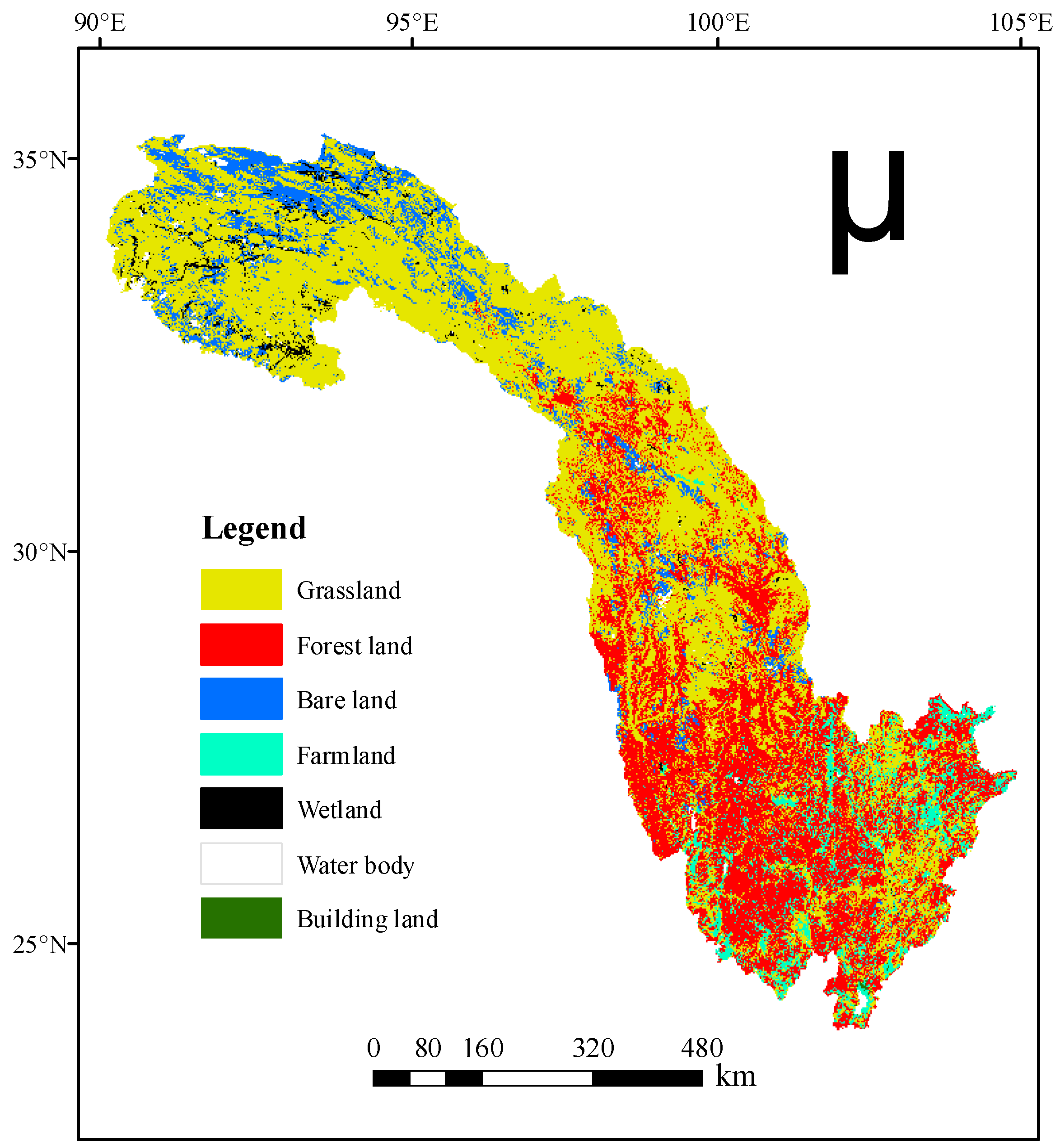
In this study, the land use in the Jinsha River Basin is divided into seven categories: grassland, forest land, bare land, farmland, wetland, water body and building land, among which the dominant land-use types are grassland and forest land, accounting for more than 80% of the whole basin area. Figure 2 displays the land-use distribution in 1980.

2.2. Materials

A wide variety of data are used in this study.

Table 1. Detailed description of research data used in this study.

Data Type	Description	Origin
Digital Elevation Model (DEM) data	Spatial resolution of 200 m	Geospatial Data Cloud (http://www.gscloud.cn)
Land-use data	In year 1980, 1990, 2000, 2015 with spatial resolution of 1000 m	Resource and Environment Data Cloud Platform (http://www.resdc.cn)
Land soil data	China Soil Map Based on Harmonized World Soil Database (v1.1) with spatial resolution of 1000 m	Cold and Arid Regions Sciences Data Center at Lanzhou (http://westdc.westgis.ac.cn)
Daily runoff in 1960–2017	9 hydrological stations uniformly distributed in the basin, including Zhimenda, Batang, Shigu, Yajiang, Luning, Xioadeshi, Panzhihua, Huatan and Pingshan	Changjiang Water Resources Commission of the Ministry of Water Resources
Daily meteorological data in 1960–2017	Daily precipitation, min/ max/average temperature, relative humidity, solar radiation and wind speed from 30 weather stations	National Meteorological Information Center (http://data.cma.cn)
General Circulation Models (GCMs) data	Daily precipitation and min/max temperature are used. Respectively 4 and 3 typical GCMs under representative concentration pathway (RCP) scenarios 4.5 and 8.5 are selected from over 20 GCMs.	Lawrence Livermore National Laboratory (https://esgf-node.llnl.gov)

provides a detailed description of various types of data, including the periods, spatial and temporal resolutions and the sources. Among them the digital elevation model (DEM) data, land use data, land soil data, meteorological data and runoff data are used for SWAT model construction and analysis of hydro-meteorological elements. Additionally, two characteristic databases of the study area are built: land soil database and meteorological database. The former is obtained from the raster map of land soil in the study area combined with the characteristic soil parameters provided by the Harmonized World Soil Database (HWSD), and the latter is acquired from the historical measurement of meteorological stations.

As for the GCM data, it is mainly used to predict future climate conditions and then to drive the hydrological model to generate future runoff processes. In this study, only the precipitation and temperature from GCMs are adopted, for the reason that they are the most important climatic factors affecting hydrological processes. Eventually, the tool of Weather Generator incorporated in the SWAT model is adopted to simulate the other climate factors (relative humidity, solar radiation, and wind speed) based on the regional meteorological database.

3. Methodology

3.1. Hydrological Modeling

SWAT is a physically based distributed hydrological model developed by the Agricultural Research Service of the United States Department of Agriculture (USDA-ARS) in the early 1990s. SWAT is able to simulate and predict the long-term hydrological cycle under different land use, soil types and management practices over large scale complex watersheds [48,49,50,51,52]. In SWAT, sub-basins are firstly divided based on the DEM, and are then further subdivided into a series of hydrological response units (HRUs) according to the topography, land use and soil types of the study area. The HRUs are the minimum calculation units, where the hydrological components including evapotranspiration (ET), interception, percolation, surface runoff and groundwater flow are calculated separately based on the water balance equation. Then the basin runoff is obtained through the overland flow and the river network confluence [53].

In this research, the SWAT model is used for daily runoff simulation in the Jinsha River Basin, and in total 33 sub-basins and 553 HRUs for the land use in 1980 were divided. The Penman-Monteith formula [54,55], the Soil Conservation Service (SCS) curve number method [56] and the Muskingum method [57] are separately employed to estimate the potential evapotranspiration (PET), the surface runoff and the routing of river network. In order to improve the performance of SWAT model simulation, the Sequential Uncertainty Fitting version 2 (SUFI2) algorithm [48] which is incorporated into the SWAT Calibration and Uncertainty Programs (SWAT-CUP) is adopted for parameter optimization. The calibration and verification periods are respectively set to be 1970–1990 and 1991–2008, with the Nash–Sutcliff coefficient (NS) and the percent bias (PBIAS) both used as indicators for assessment of simulation effects.

3.2. Trend Detection of Hydro-Meteorological Series

The Mann–Kendall (M–K) method, which is originally proposed by Mann and Kendall [58,59], is a nonparametric statistical method recommended by the World Meteorological Organization (WMO) and has been widely used in practice to evaluate the significance of monotonic trends in hydro-meteorological time series [60]. It possesses the advantages of not requiring the sample to follow a certain distribution, not being interfered by a few abnormal values, and simple calculation. For this reason, it is employed for trend analysis of hydro-meteorological series in this research, and the 95% confidence level is adopted with the threshold of standard normal statistics Z_MK equal to ±1.96.

It is well-known that the Mann–Kendall test relies purely on statistical results, which might not make sense all the time. To address this problem and reinforce the findings, the cumulative sum of rank difference (CSD) test method, which was recently proposed by Onyutha [61,62,63,64], is also employed for the trend analysis of hydro-meteorological series in this research. The advantage of the CSD method over the other tests such as the Mann–Kendall test is that it takes into account the graphical diagnoses and statistical analyses of the data series comprehensively. In the CSD test, Z_CSD denotes the standardized trend statistic, and a positive/negative value of Z_CSD indicates an upward/downward linear trend. Given a significance level of αs%, the null hypothesis H₀ (no trend) is rejected if |Z_CSD| ≥ |Z_αs/2|. In this research the 95% confidence level is adopted with the threshold of standard trend statistic Z_CSD equal to ±1.96.

3.3. Indicators of Hydrologic Alteration

Developed by the US Nature Conservancy (TNC), the indicators of hydrologic alteration (IHA) approach [65,66,67] is a practical tool for calculating the characteristics of natural and altered hydrological regimes [68]. It compares hydrological data sets by calculating multi-variate statistics to assess the degree of hydrological alteration [69]. A total of 67 statistical parameters closely related to river ecosystems are calculated in the IHA approach, which are divided into two groups: 33 IHA parameters and 34 environmental flow component (EFC) parameters. In recent years, it has been widely used to evaluate the degree of hydrological alteration under the impacts of climate change and anthropogenic activities such as water conservancy projects and land use change [70,71,72].

In this research, several IHA parameters and EFC parameters associated with extreme hydrology are employed. Based on the daily hydrological series, the annual values of extreme hydrologic indicators are calculated using IHA tool for subsequent analysis. The water year starts on 1 January and ends on 31 December. The parametric statistics are adopted with the high and low pulse thresholds defined as the mean plus or minus 1 standard deviation, and a day is classified as a high/low pulse if it is greater/lower than these thresholds. All flows that exceed 75% of daily flows for the period are classified as initial high flows, and all flows below this level are classified as initial low flows. A flood event is defined as an initial high flow with a flow peak greater than two-year return interval event, and an initial low flow below 10% of daily flow are classified as an extreme low flow event.

3.4. Separating the Impacts of Climate Change and Land-Use Change

In order to distinguish the impacts of climate change and land-use change on hydrological extremes quantitatively, the historical measured land use and climate data are respectively subdivided into four periods, which are mutually combined to formulate 16 scenarios (

Table 2. Four research periods extracted from the historical period (1970–2017) and the corresponding climate and land-use datasets.

Periods	P1	P2	P3	P4
Climate data	1970–1984	1985–1994	1995–2004	2005–2017
Land-use data	LU1980	LU1990	LU2000	LU2015

and

Table 3. The setting of 16 scenarios combining historical measured climate and land-use data in different periods.

Scenarios	Climate Data	Land Use Data	Scenarios	Climate Data	Land Use Data
S1	1970–1984	LU1980	S9	1995–2004	LU1980
S2	1970–1984	LU1990	S10	1995–2004	LU1990
S3	1970–1984	LU2000	S11	1995–2004	LU2000
S4	1970–1984	LU2015	S12	1995–2004	LU2015
S5	1985–1994	LU1980	S13	2005–2017	LU1980
S6	1985–1994	LU1990	S14	2005–2017	LU1990
S7	1985–1994	LU2000	S15	2005–2017	LU2000
S8	1985–1994	LU2015	S16	2005–2017	LU2015

). By means of SWAT model, the runoff series for each scenario are obtained and the corresponding extreme hydrological indicators are derived.

Two relative action factors are recommended in this study to quantitatively separate the impacts of climate change and land-use change on hydrological extremes. They are P^′_LU and P^′_CC, which are calculated as follows:

$$P_{LU}^{\prime }=\frac{\Delta X_{LU}}{\Delta X}$$

(1)

$$P_{CC}^{\prime }=\frac{\Delta X_{CC}}{\Delta X}$$

(2)

where ∆X is the increase in hydrological extremes under the combined effects of the two factors, while ∆X_LU and ∆X_CC represent the increase due to land-use change and climate change respectively. In order to make the two factors added up to be 100 percent, a redistribution between P^′_LU and P^′_CC is performed:

$$P_{LU}=P_{LU}^{\prime }/\left(P_{LU}^{\prime }+P_{CC}^{\prime }\right)$$

(3)

$$P_{CC}=P_{CC}^{\prime }/\left(P_{LU}^{\prime }+P_{CC}^{\prime }\right)$$

(4)

$$P_{LU}+P_{CC}=100\%$$

(5)

where P_LU and P_CC are respectively defined as the attribution proportions of land-use change and climate change which lead to the variations in extreme hydrological indexes.

3.5. Downscaled CMIP5 (Coupled Model Inter-Comparison Project Phase 5) Simulations

By means of a statistical downscaling method named DBC and a distributed hydrological model called SWAT, this study targets at evaluating the evolution trends of hydrological extremes in the near future (2021–2050) using CMIP5 (Coupled Model Inter-comparison Project Phase 5) ensemble simulations (Historical + RCP4.5/RCP8.5). Originally proposed by Jie Chen et al. [73,74], the DBC method assumes same deviations in each quantile between future and historical climate. It combines the local intensity scaling (LOCI) method and daily translation (DT) method to take into account the precipitation occurrence and the frequency distributions of precipitation amounts and temperatures. In this study, the historical observed precipitation and min and max temperature in 1960–2005 are used for bias correction.

4. Results and Discussion

4.1. Trend Analysis of Historical Data

4.1.1. Hydro-Meteorological Data

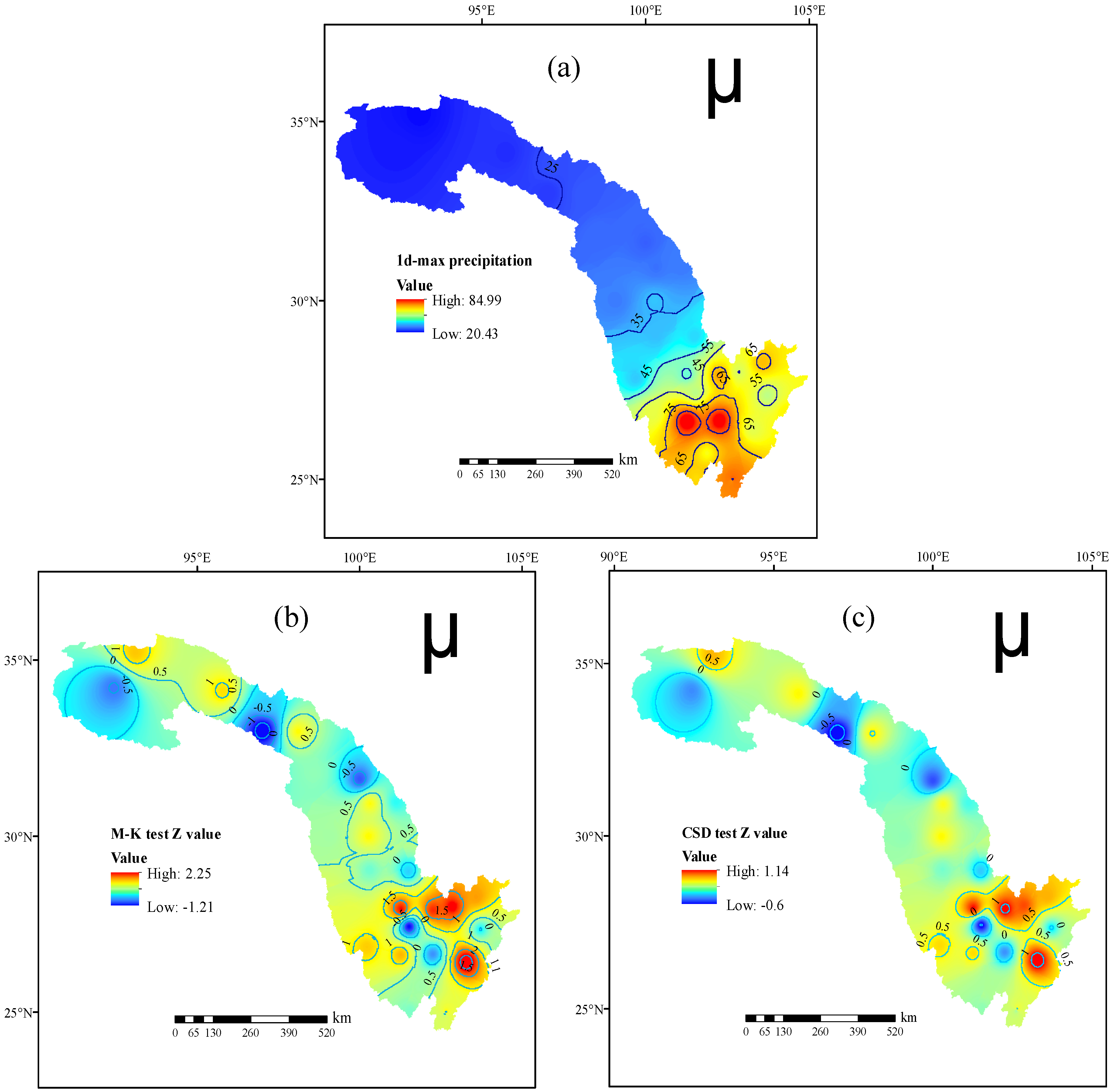
The annual maximum 1-day precipitation and the Z values from M–K as well as CSD trend test for each rainfall station is calculated and interpolated using the inverse distance weighting (IDW) method to obtain the spatial distribution (Figure 3). The IDW method is one of the most commonly used techniques for the interpolation of scatter points, which is based on the concept of distance weighting. It is simple to use and clear in physical meaning [75,76]. It can be seen from Figure 3a that the maximum 1-day precipitation increases gradually from upstream to downstream. In the upper reaches of the Jinsha and Yalong River, the values are generally smaller (20–40 mm), and they are highest at the confluence of the two rivers, which is approximately 80 mm. During the past 58 years, similar trends have been detected using the two test methods, except that the absolute values of Z from M–K test are generally greater than that of CSD test, as shown in Figure 3b,c. The two tests yield the same conclusion that the annual maximum 1-day precipitation is generally dominated by increasing trends in the basin (Z > 0 for most regions). Besides, under a 95% confidence level none of the rainfall stations reaches a significant level for the CSD test, while significant upward trends (Z > 1.96) are detected in the southeastern part of the basin for the M–K test. Overall, the Z values in the southeastern part of the basin are obviously higher for both test methods, indicating rising risks of extreme precipitation in the lower reaches of the Jinsha River Basin.

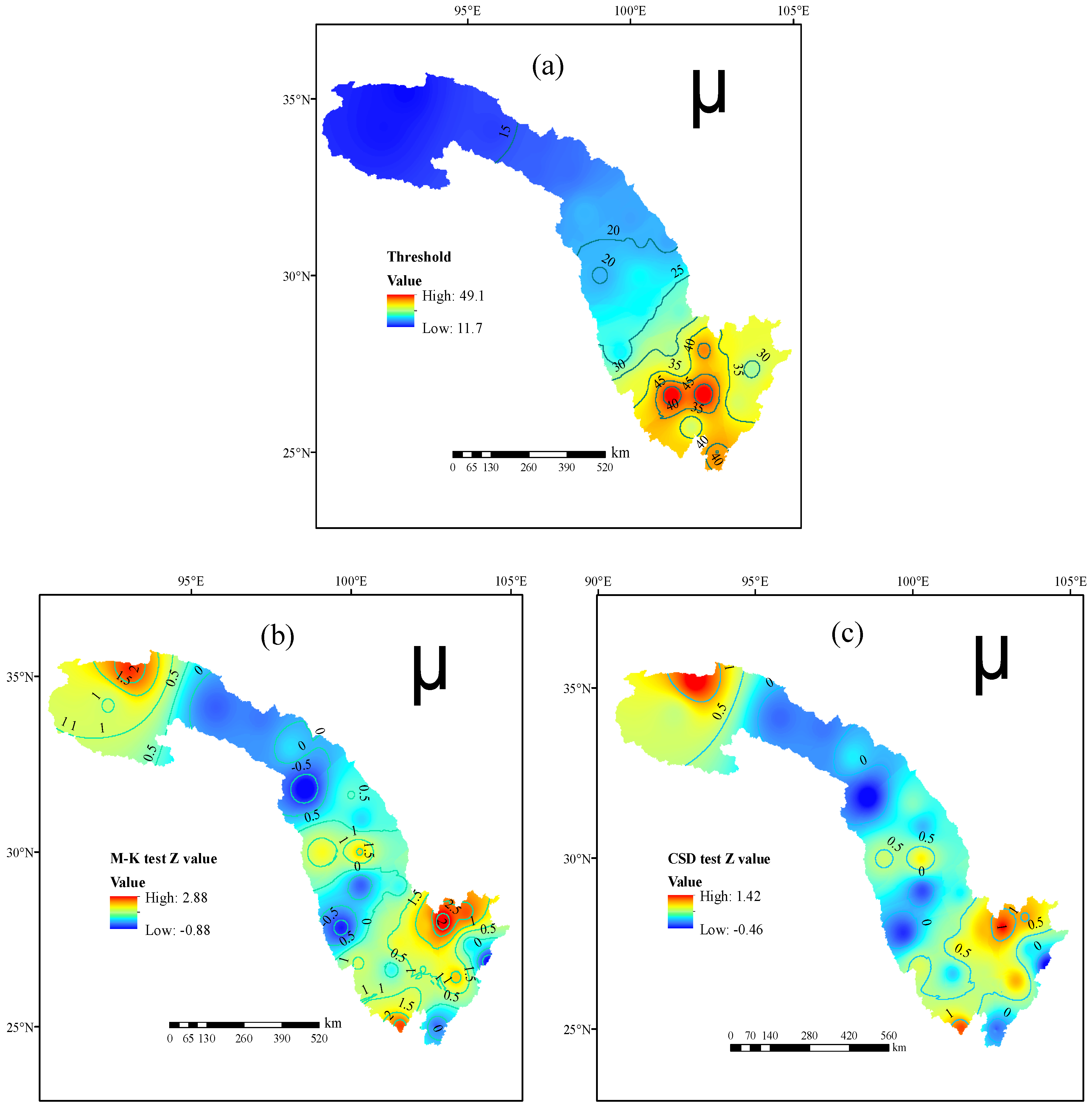
For each rainfall station, the 99% quantile of daily precipitation is selected as the threshold of extreme precipitation, and the extreme precipitation frequency is defined as the days exceeding this threshold in a year. The spatial distribution of extreme precipitation thresholds are displayed in Figure 4a. In the southeastern region the thresholds are about 30–45 mm, which is significantly higher than the northwestern (about 15 mm) and central (about 20 mm) parts. It shows that the extreme precipitation intensity gradually increases from upstream to downstream in the basin, which is consistent with Figure 3a. Meanwhile, extreme precipitation frequency was counted at each rainfall station from 1960 to 2017, and two trend tests (M–K and CSD) were conducted. The spatial distributions of Z values from the two tests are obtained through interpolation using the IDW method, shown in Figure 4b,c. Results show that the extreme precipitation frequency in the Jinsha River Basin has been dominated by increasing trends during the past 58 years (Z > 0 for most stations, of which four stations reaches a significant level for M–K test). In the southeastern and northwestern parts of the basin, increasing frequency of extreme precipitation is detected for both M–K and CSD tests.

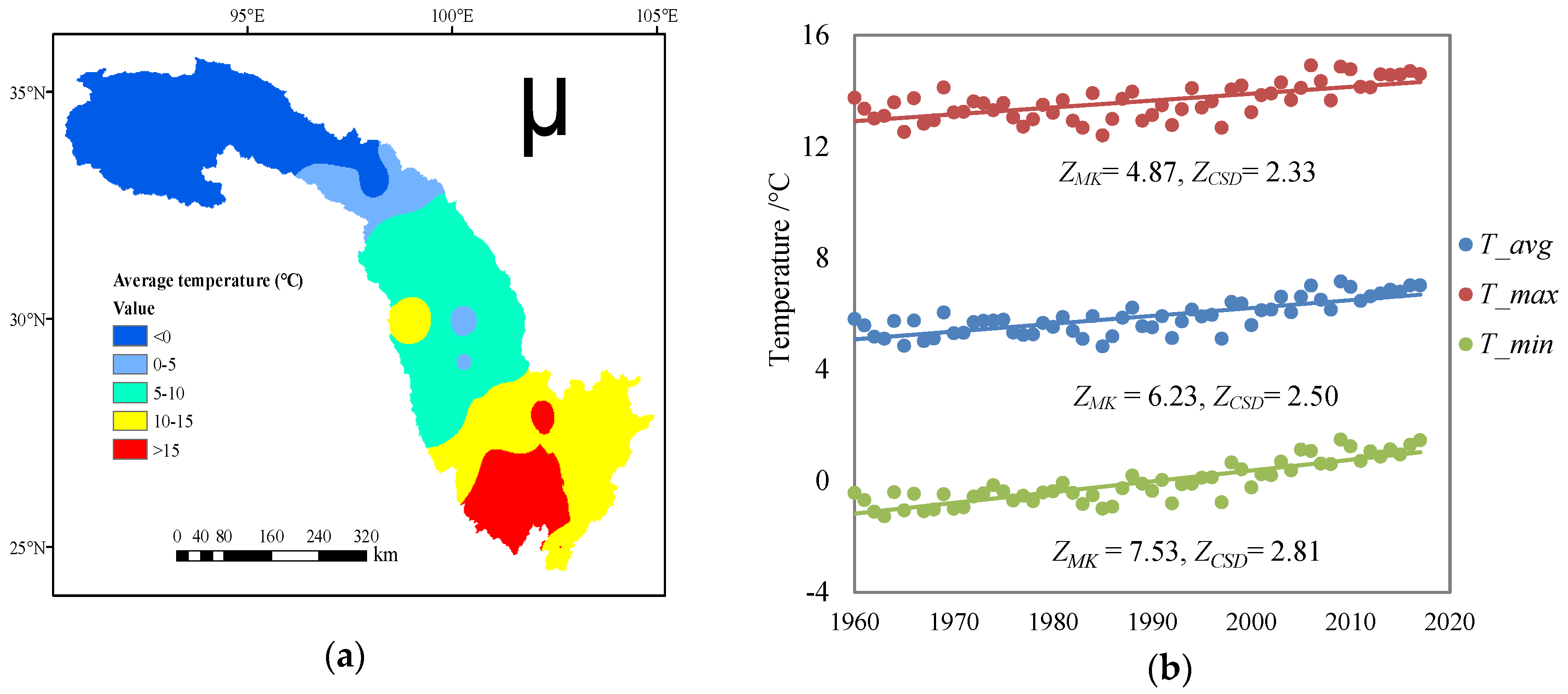
By means of Thiessen Polygon method, the annual averaged max, min and average temperature are respectively calculated to be 13.6 °C, −0.1 °C and 5.9 °C in the Jinsha River Basin during 1960–2017. The special topography and climate condition in the basin have created the significant spatial differences in temperature (Figure 5a). The average temperature is below 0 °C in the northwestern part of the basin, while in some southern parts it is higher than 15 °C. From Figure 5b it can be found that all the max, min and average temperature have increased significantly during the past 58 years (Z > 1.96 for both M–K and CSD tests). Meanwhile, the rising trend of min temperature is more significant than that of max temperature (Z values for T_min is larger than that of T_max).

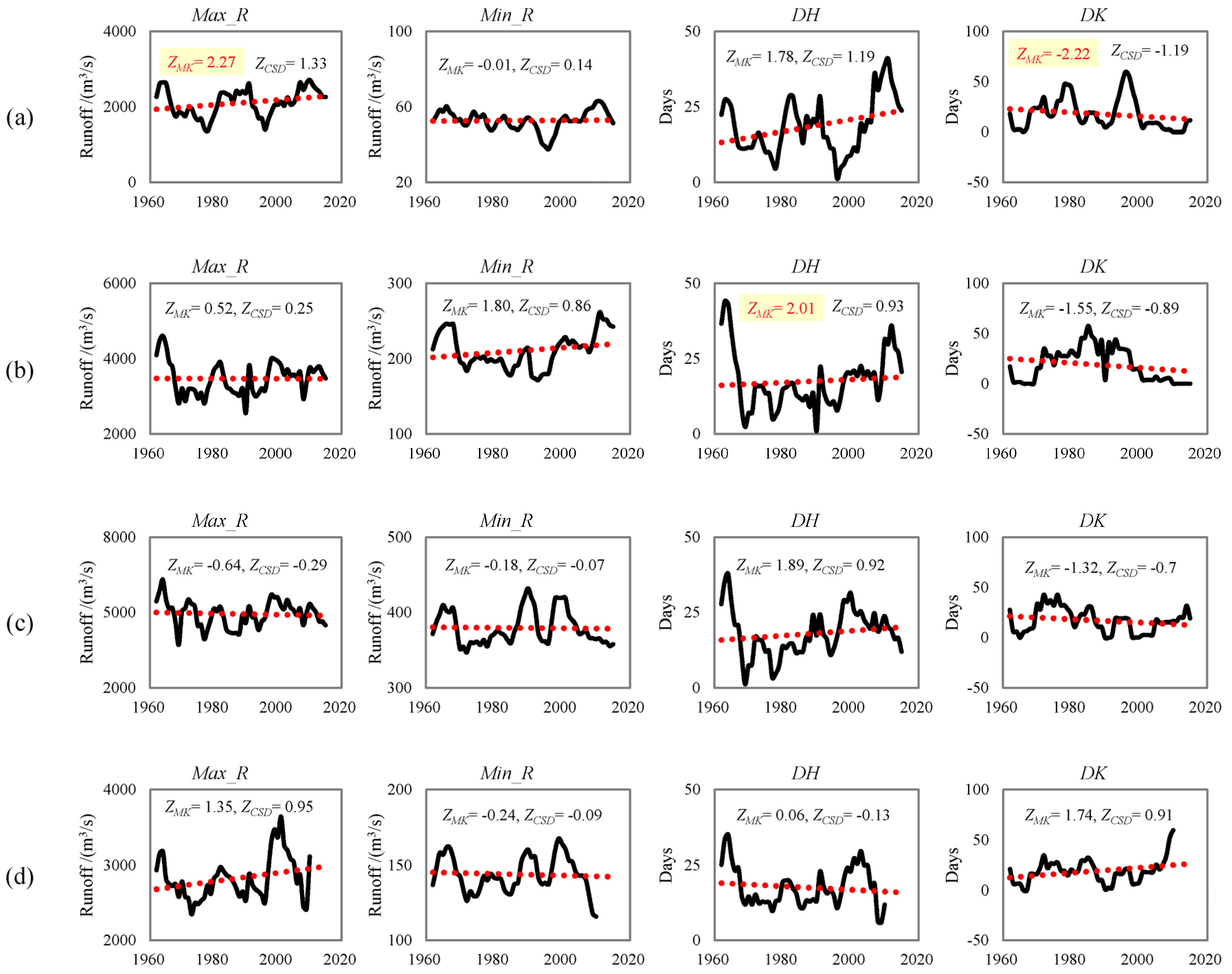
In order to characterize the spatial-temporal variations of runoff extremes in the Jinsha River Basin, the daily runoff data for the period 1960–2017 from nine hydrological stations, which are uniformly distributed in the basin is adopted. Four indicators are selected to characterize the runoff extremes, including annual maximum and minimum runoff (Max_R, Min_R), flood and dry days (DH, DK). The thresholds of DH and DK are respectively determined by the 95% and 5% quantiles of the daily runoff series.

It should be pointed out that plenty of factors, such as limited sources, data missing and water conservancy projects, have resulted in the incompleteness of runoff observation in most hydrological stations, which brought challenges to trend analysis of extreme hydrological indicators during the historical period. To make the best use of existing materials and ensure statistical accuracy, the method of linear interpolation between adjacent measured data is employed for runoff series with no more than 10 days of continuous missing values. Years with more missing data are excluded from statistics. Thus the annual series of extreme hydrological indexes with high reliability in 1960–2017 are obtained. Finally, in order to eliminate the interference of a few outliers and highlight the inter-annual trend of the indicators, the moving average for a 5-years’ step is performed for each index. Detailed information of the runoff observation is listed in

Table 4. Detailed descriptions of runoff data at 9 hydrological stations in the Jinsha River Basin.

Location	Hydrological Stations	Notes
Upstream of Jinsha River	Zhimenda	The runoff is measured every 10 days in dry seasons of 2009–2016
	Batang	Missing runoff data in year 1969–1970, 1989–1991 and 2009–2010
	Shigu	Missing runoff data in year 1969–1970
Yalong River	Yajiang	Missing runoff data in year 1969 and 2009–2017
	Luning	Missing runoff data in dry seasons of 2009–2017
	Xiaodeshi	Missing runoff data in year 2011–2017; River cutoff during 4 to 7 May 1998 due to engineering reasons
Middle and downstream of Jinsha River	Panzhihua	Missing runoff data from 1 January 1960 to 9 May 1965
	Huatan	Missing runoff data in year 1960–1976; The runoff data after 3 August 2015 is derived from Baihetan hydrological station; Sudden drops in runoff occurred in 9–10 December 2015 due to engineering reasons
	Pingshan	The runoff data in year 2012–2016 and 2017 respectively comes from Xiangjiaba hydrological station and the inflow of Xiangjiaba reservoir

Note: The dry season of a certain year is defined as October to the next April.

.

Figure 6 displays the temporal variations of extreme runoff indicators in the Jinsha River Basin during the period of 1960–2017, with Z values from M–K test (Z_MK) and CSD test (Z_CSD) labelled. Results indicated that, (1) the two trend test methods are very consistent in the evaluation of changing directions of data series. However, the CSD test is more rigorous in assessing significance than the M–K test under the same confidence level, which is reflected by the fact that the M–K test will always reach a significant level (|Z| > 1.96) as long as the CSD test does. The main reason for this realization is that when series are characterized by persistent fluctuations, the differences among trend detection methods become large [63]. Therefore, there is a need to consider a number of tests for trend analyses (as done in this study) to reduce the uncertainty of the results due to selection of a particular method. (2) Focusing on the indicator of flood days (DH), it can be found that all hydrological stations show increasing trends, except for Yajiang and Pingshan stations. The DH values at Luning, Xiaodeshi, Panzhihua, Huatan and Pingshan stations have decreased significantly since the 21st century. This may be explained by the reservoir regulations, which exert a peak-clipping effect on river runoff. In summary, regardless of water conservancy projects, the DH values have generally increased in the basin, indicating rising risk of floods over the past 58 years. This result is consistent with the analysis of extreme precipitation. (3) Seven hydrological stations show decreasing trends (Z < 0) for the indicator of dry days (DK), and respectively three and one of them reach significant level (Z < −1.96) for M–K and CSD test. For Huatan and Pingshan stations, which are located in the lower reaches of the Jinsha River, the decreasing trends are particularly evident. The water conservancy projects might contribute to the decline of DK, for the reason that DK remained comparatively stable at a relatively low level since the 21st century. On the other hand, for the three stations located in the upper reaches of the Jinsha River (Zhimenda, Batang and Shigu), which are affected by human activities very little, the decreasing trends are also observed in DK, reflecting decreased risk of droughts regardless of the impacts of water conservancy projects.

For each extreme runoff indicator, the number of hydrological stations at which the indicators show increasing or decreasing trends during 1960–2017 are respectively counted (

Table 5. Statistics of two trend test results of 4 extreme runoff indicators in 9 hydrological stations in the Jinsha River Basin.

Numbers of Hydrological Stations	Max_R		Min_R		DH		DK
	Positive	Negative	Positive	Negative	Positive	Negative	Positive	Negative
M–K test	5(1)	4(1)	4(1)	5(2)	8(2)	1(0)	2(1)	7(3)
CSD test	5(0)	4(0)	5(0)	4(2)	7(0)	2(0)	2(1)	7(1)

Note: the numbers in parentheses represent the number of hydrological stations that reach a significant level.

). Almost equivalent numbers of hydrological stations show increasing and decreasing trends for the indexes of Max_R and Min_R, indicating there is no common changing direction for these two indexes. In contrast, the indicators of DH and DK respectively show a general upward and downward trend, which are consistent with the analytical results in Figure 6. In summary, the flood risk in the Jinsha River Basin has generally increased during 1960–2017, to which attention should be paid, while the risk of droughts has declined in a certain degree.

4.1.2. Land-Use Data

The areas of various land use types as well as the changing rates over the past 35 years in the Jinsha River Basin are listed in

Table 6. The areas of various land use types as well as the changing rates over 1980–2015 in the Jinsha River Basin.

Land Use	Annual Average Area (103 km2)	Proportion (%)	Change Rates (%)
			1980–1990	1990–2000	2000–2015
Grassland	234.3	52.53	0.17	0.10	−0.19
Forest land	132.4	29.68	−0.24	−0.26	0.04
Bare land	41.9	9.40	−0.10	0.22	−0.03
Farmland	26.5	5.94	−0.26	−0.30	−2.81
wetland	6.91	1.55	0.38	−0.60	−0.04
Water body	3.50	0.78	−0.61	3.08	10.02
Building land	0.55	0.12	5.95	8.99	227.06

. It can be found that the main land use types are grassland and forest land, and the areas of different land use types have changed little during 1980–2015, except for water body and building land. The farmland continues to shrink at a relatively slow rate. Affected by water conservancy projects, the water body in the basin has expanded rapidly since the 1990s. The building land continues to grow during 1980–2015, and the area has surged by 227.06% since the 21st century. Therefore, a conclusion can be drawn that there are great changes in the areas of building land and water body in the Jinsha River Basin. However, attention should be paid to the fact that these two kinds of land-use types occupy a very small proportion of the whole basin area. The land-use changes in the Jinsha River Basin during the period of 1980–2015 are thoroughly analyzed by Qihui Chen et al. [77].

4.2. Evaluation of Runoff Simulation Effects

In this research, the analyses of hydrological extremes are mostly based on the SWAT simulations and downscaled GCMs outputs. To achieve reliable research results, the evaluations of runoff simulation effects of the SWAT model and GCM data are necessary. Through comparison of the simulated and observed runoff during the calibration and verification period (1970–2008), the simulation effects of SWAT model is assessed. The performance of downscaled GCMs data in runoff simulation is evaluated by comparing SWAT application with the climate model outputs and SWAT application with observed meteorological data for the reference period (1970–2005). At the same time, the land-use data in year 1980 are used.

The indicators of hydrologic alteration (IHA) method is adopted to assess the deviations of runoff series, and the deviation factor (DF) is used as the evaluation indicator. Totally 18 parameters are selected as the characterization of runoff extremes, including 14 IHA parameters (annual 1, 3, 7, 30, 90-day max/min, Julian date of 1-day max/min, high pulse frequency and duration) and 4 EFC parameters (the frequency and duration of floods/extreme low flows). The average values of each parameter for the evaluated and reference runoff series is separately calculated, thus the DF values can be obtained following this formula:

DF = |(Mean of evaluated series) − (Mean of reference series)|/(Mean of reference series)

(6)

For each hydrological station, the DF values for the 18 extreme runoff indicators are calculated. Smaller DF values represent better simulation effects on the runoff extremes, and vice versa. In this study, pretty good simulation effects are believed to result when the DF values are within 0.2, while bad simulation effects are considered when the DF values are greater than 0.5.

4.2.1. Simulation Effects of Soil and Water Assessment Tool (SWAT) Model

A daily-scale hydrological model called SWAT is established in the Jinsha River Basin, with the calibration and verification period respectively set to be 1970–1990 and 1991–2008.

Table 7. Simulation effects of the soil and water assessment tool (SWAT) model on runoff processes in the Jinsha River Basin.

Hydrological Stations		Calibration Period (1970–1990)		Verification Period (1991–2008)
		NS	PBIAS (%)	NS	PBIAS (%)
Upstream of Jinsha River	Zhimenda	0.68	−3	0.67	−17.6
	Batang	0.82	0.1	0.86	−7.1
	Shigu	0.85	11.4	0.89	4.7
Yalong River	Yajiang	0.86	−2.2	0.85	2
	Luning	0.9	−1.2	0.89	4.4
	Xiaodeshi	0.88	8.2	0.79	13.9
Middle & downstream of Jinsha River	Panzhihua	0.89	−4.1	0.9	−8.7
	Huatan	0.91	−3.7	0.89	0.1
	Pingshan	0.89	2.2	0.88	−0.5
Absolute average mean		0.85	4	0.85	6.6

shows the simulation effects of the SWAT model on the runoff processes of nine hydrological stations, whose geographic locations are displayed in Figure 1. In this research the Nash–Sutcliff coefficient (NS) and the percent bias (PBIAS) are both selected as evaluation indicators.

It can be seen from Table 7 that: (1) the simulation effect of Zhimenda station is not satisfying, with NS values less than 0.7 and the absolute value of PBIAS exceeding 15% in the verification period. This might be explained by the rather complicated hydrological processes due to particular topographic and climatic conditions over the drainage area, where the rainfall and snow melt both serve as the main sources of runoff. (2) For all the hydrological stations except Zhimenda, the NS and PBIAS values are respectively greater than 0.8 and within ±15%. In addition, affected by the construction of Ertan Hydropower Engineering, the runoff series at Xiaodeshi station was significantly disturbed since 1998, resulting in a relatively smaller value of NS during the verification period. (3) The absolute average values of NS and PBIAS of the nine hydrological stations respectively achieve 0.85 and are within 10% both in the calibration and verification periods. It indicates that the SWAT model has a good simulation effect on the runoff processes in the Jinsha River Basin.

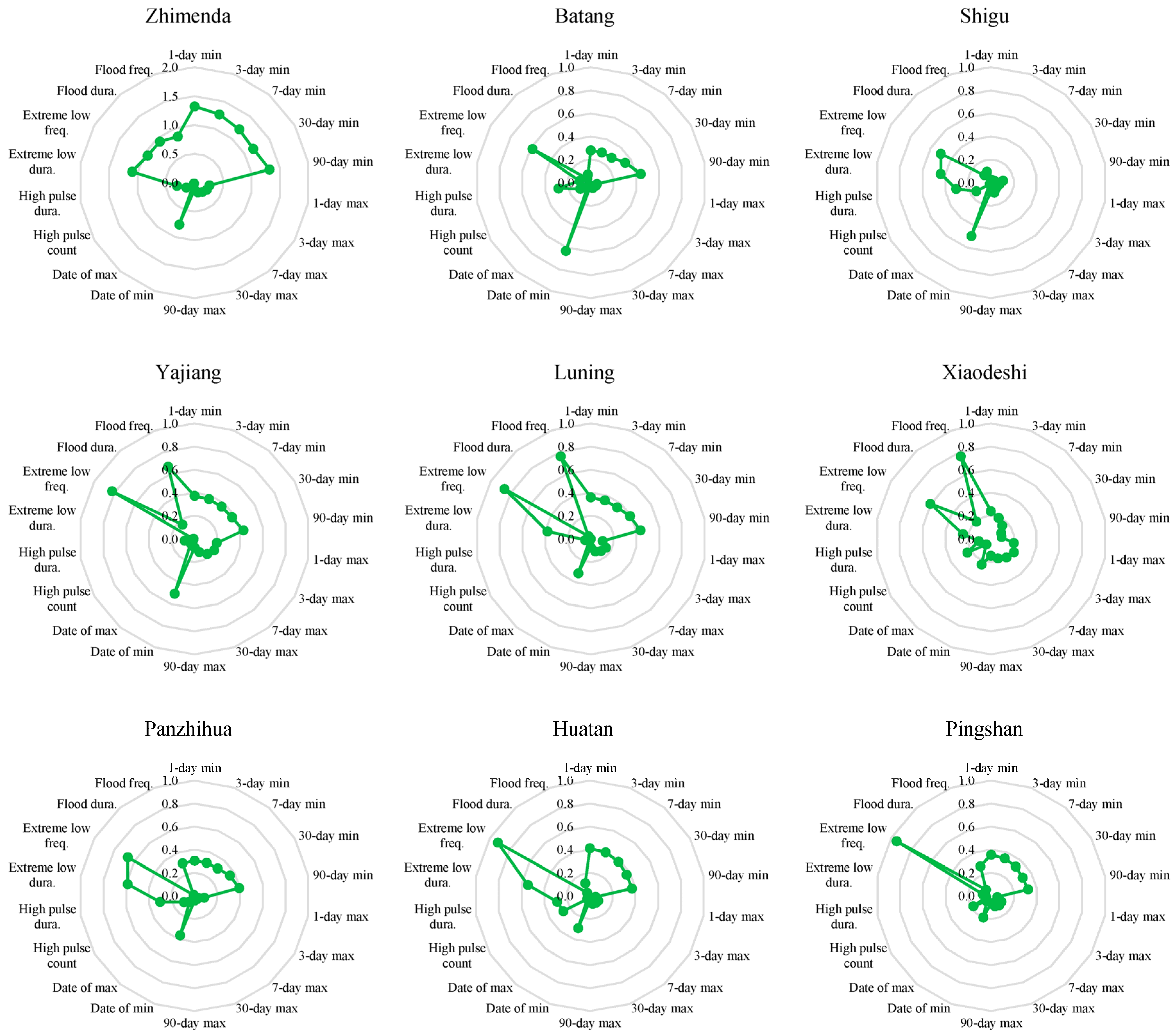
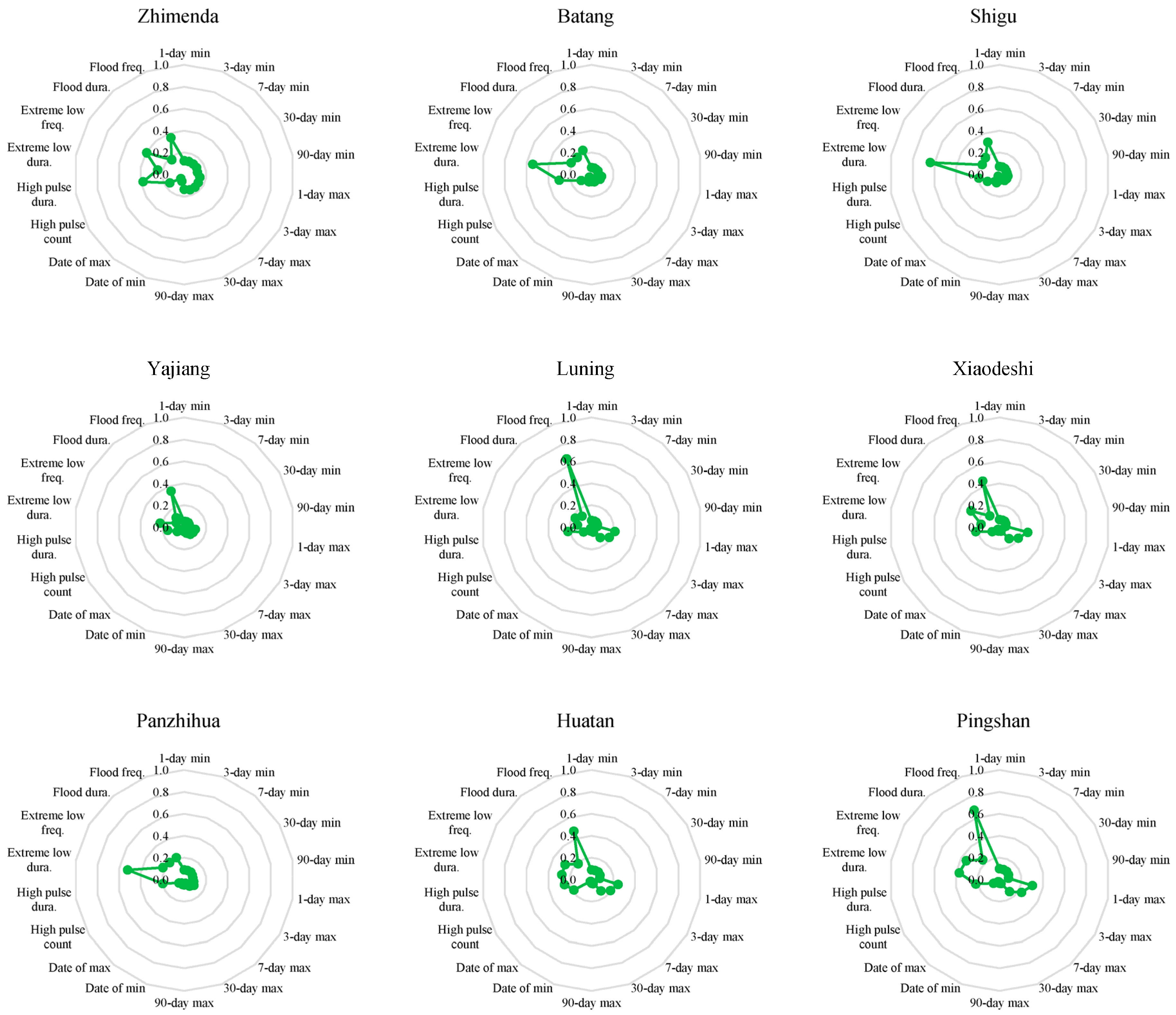
To assess the SWAT simulation effects on hydrological extremes, the simulated and observed runoff in the Jinsha River Basin during 1970–2005 are compared using IHA method, with the deviation factor (DF) used as the evaluation indicator. Figure 7 displays the DF values for each hydrological station. There are 18 extreme runoff indicators at the circumference, and the radius of each point represents the corresponding DF value.

As can be seen from Figure 7, the simulation effects of eight parameters are pretty good with DF values generally within 0.2. They are annual 1, 3, 7, 30, 90-day max, Julian date of 1-day max, high pulse frequency and duration of floods. Whereas the simulation effects are relatively poor for the other parameters, especially for the extreme low frequency, flood frequency and date of min, whose DF values are generally higher than 0.5. Among the nine hydrological stations, Shigu achieves the best simulation effect on the runoff extremes, followed by Pingshan, Batang, Panzhihua, Luning and Xiaodeshi stations. Meanwhile, the simulation effect of Zhimenda station is rather poor. In general, the SWAT model has a good simulation effect on high flows but a poor simulation effect on extreme low flows in the Jinsha River Basin.

4.2.2. Performance of General Circulation Model (GCM) Data in Runoff Simulation

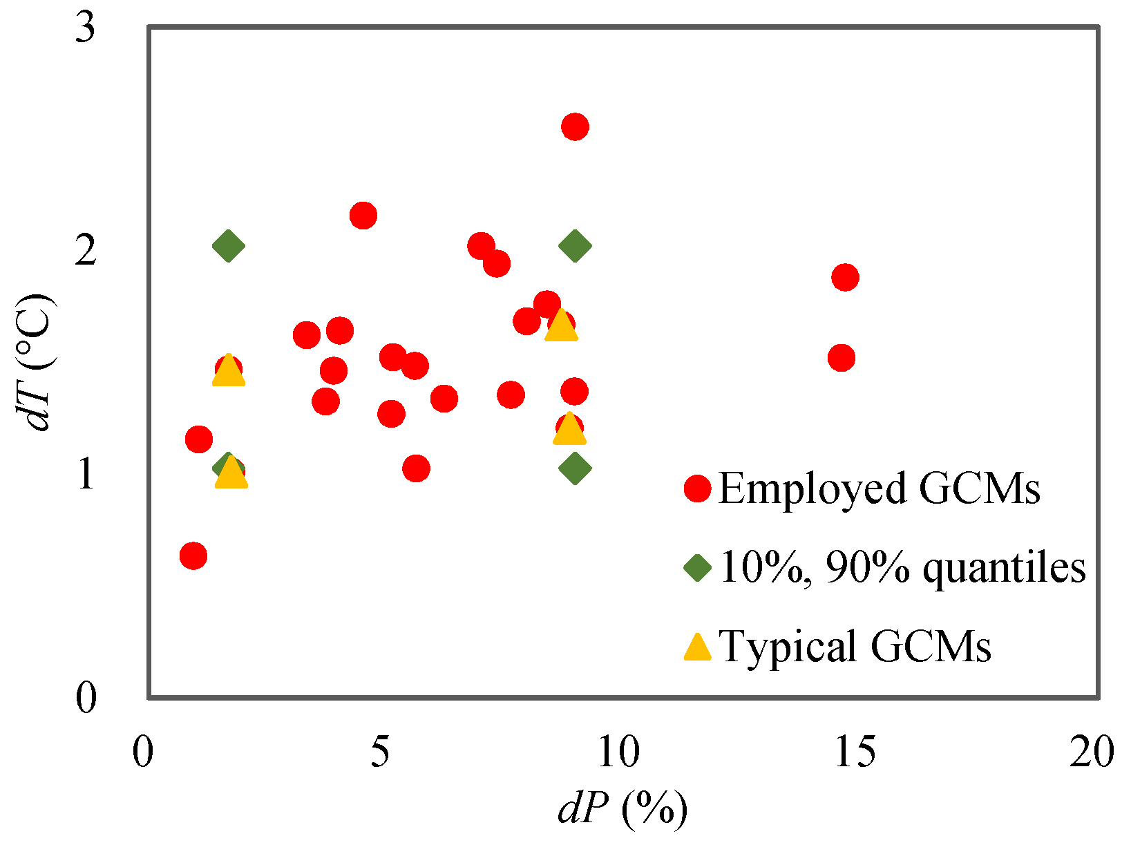
In this research, respectively 25 and 28 GCMs under RCP4.5 and RCP8.5 emission scenarios from CMIP5 are taken into account. To avoid information redundancy as well as to simplify the subsequent analysis, a set of typical GCMs which can well represent the future climate characteristics of this basin are selected with a specific method [78]. Based on the 10% and 90% quantiles of the changes in precipitation and temperature in the predicted period (2021–2050) compared with the reference period (1970–2005), respectively four and three typical GCMs under RCP4.5 and RCP8.5 emission scenarios are selected in this research. Taking the selection of typical GCMs under RCP4.5 emission scenario as an instance (Figure 8), the red dots represent the results of 25 corrected GCMs. The 10% and 90% quantiles of dP (%) and dT (°C) are calculated separately, forming four vertices represented by the green dots, which stand for the ideal warm-dry, warm-wet, cold-dry and cold-wet climate scenarios in the future. The specific GCMs closest to the four vertices are selected as typical GCMs for this basin, as shown by the four yellow points.

Table 8. Typical GCMs selected under the two emission scenarios with the corresponding spatial resolutions listed. The outputs of each typical GCM respectively representing the typical climate scenarios of cold-dry, cold-wet, warm-dry and warm-wet.

Climate Models	RCP4.5		RCP8.5
	Typical GCMs	Spatial Resolution	Typical GCMs	Spatial Resolution
Cold-dry	IPSL-CM5B-LR	3.75° × 1.90°	CSIRO-Mk3-6-0	1.875° × 1.875°
Cold-wet	GFDL-ESM2M	2.5° × 2.0°	CCSM4	1.25° × 0.94°
Warm-dry	CMCC-CM	0.75° × 0.75°	CSIRO-Mk3-6-0	1.875° × 1.875°
Warm-wet	BNU-ESM	2.8° × 2.8°	MIROC-ESM	2.8° × 2.8°

Note: Under RCP8.5 emission scenario, the GCMs representing future climate scenarios of cold-dry and warm-dry are the same (CSIRO-Mk3-6-0). Therefore, totally seven typical GCMs under the two emission scenarios are selected.

lists the selected typical GCMs under the two emission scenarios and the corresponding spatial resolutions.

Table 9. Deviation factors (DF) of average monthly flows of SWAT simulations using historical GCM data (1970–2005) compared with SWAT simulations using historical climate instrumentations (1970–2005) in the Jinsha River Basin.

DF Values	a	b	c	d	e	f	g	h	i
January	12.3	6.9	6.3	3.8	4.0	4.6	6.6	6.5	7.3
February	12.3	7.1	6.5	3.9	4.3	4.8	7.0	6.6	7.2
March	12.3	6.5	5.8	3.9	4.6	5.2	6.8	6.6	7.1
April	14.5	5.9	6.6	3.4	4.6	5.6	9.4	8.8	9.6
May	4.8	3.2	2.6	9.2	5.0	4.4	3.6	1.4	2.9
June	13.1	9.5	8.6	7.7	6.2	6.0	5.5	5.0	4.3
July	11.6	5.7	4.4	4.4	3.4	4.2	5.6	5.7	6.0
August	16.4	8.4	6.3	4.6	3.6	3.6	5.3	3.5	3.1
September	13.4	7.3	6.2	5.2	4.7	5.0	6.7	6.3	6.2
October	11.7	8.0	8.6	8.6	9.2	9.3	9.0	9.3	9.4
November	12.3	7.8	6.6	3.7	3.8	4.2	6.6	5.4	6.0
December	12.4	8.7	7.9	4.1	4.3	4.7	7.9	6.9	7.5

Note: The symbols a–i respectively stand for the nine hydrological stations in the basin: Zhimenda (a), Batang (b), Shigu (c), Yajiang (d), Luning (e), Xiaodeshi (f), Panzhihua (g), Huatan (h) and Pingshan (i) station.

presents the effect of historical GCM data (1970–2005) in simulating monthly runoff at the nine hydrological stations in the Jinsha River Basin with SWAT model. The DF values are calculated based on the SWAT simulations using historical climate observations (1970–2005), with the land-use data in year 1980 used as input. Seven typical GCMs under RCP4.5 and RCP8.5 emission scenarios are selected in this study, and a set of DF values for each GCM can be obtained. To summarize the results, only the average DF values of the seven typical GCMs for each indicators are presented here. From Table 9 we can see that except for Zhimenda hydrological station, the DF values at the other stations are within 10%, indicating good performance of GCM data in simulating mean values of runoff.

Similar to Table 9 above, Figure 9 displays the effect of historical GCM data (1970–2005) in simulating runoff extremes with the SWAT model. 18 extreme runoff indicators are adopted and the corresponding DF values are calculated, which are averaged for the seven typical GCMs, with the SWAT simulations using historical climate observations used as reference. It can be seen that the DF values are generally greater than 0.2 for the frequency and duration of floods and extreme low flows, indicating poor simulation effect in the characteristics of floods and extreme low flows. As for the other extreme runoff indicators, the simulation effects are all within acceptable limits.

By comprehensively taking into consideration the simulation effects of the SWAT model and the performance of GCM data in runoff simulations both in average and extreme values for each hydrological station (Table 7 and Table 9, Figure 7 and Figure 9), four extreme runoff indicators (3-day max, 3-day min, high pulse frequency and high pulse duration) as well as four hydrological stations (Batang, Panzhihua, Xiaodeshi and Pingshan) are selected to analyze the hydrological extremes in the Jinsha River Basin in the following analysis.

4.3. Quantitative Assessment of the Impacts of Climate Change and Land-Use Change on Runoff Extremes

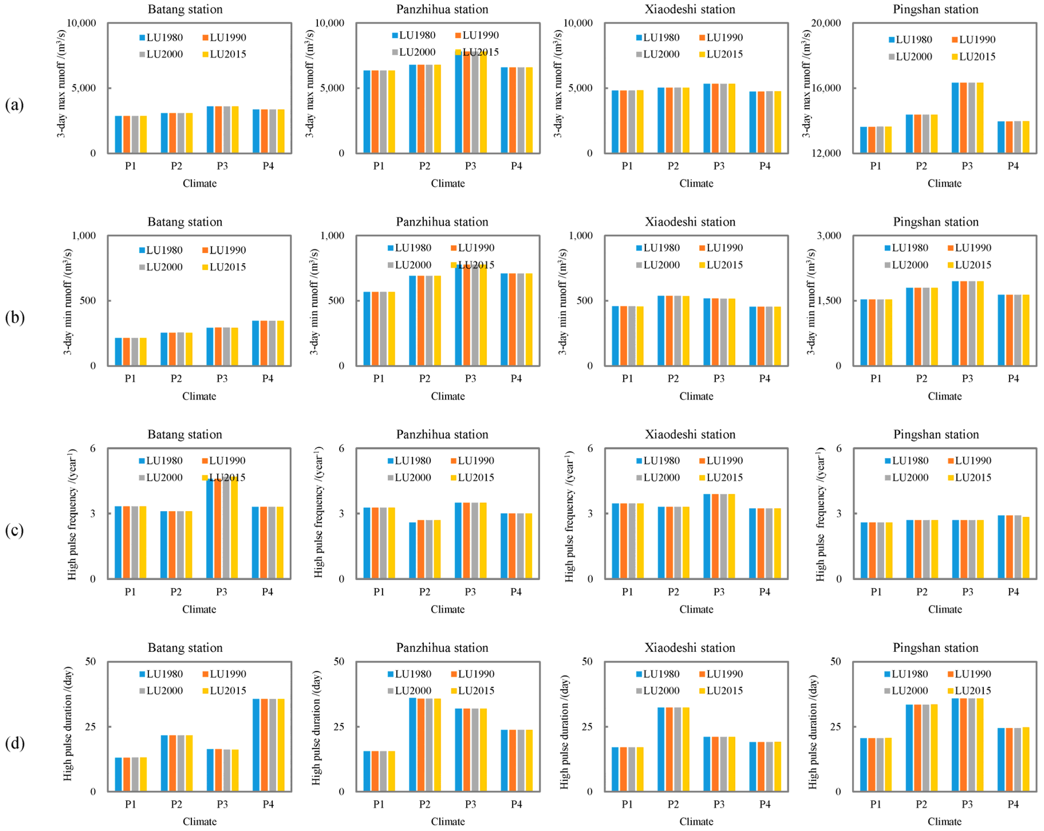
In order to quantitatively distinguish the impacts of climate change and land-use change on runoff extremes, this study respectively divides the historical measured land-use and climate data into four periods (Climate P1–P4; LU1980/1990/2000/2015). The two kinds of data are mutually combined into 16 scenarios, which are separately input into the SWAT model to simulate the corresponding runoff extremes (Table 2 and Table 3). In this research, the annual 3-day max and min runoff are used as descriptions of extreme runoff characteristics, and high pulse frequency and durations are adopted to reflect the high flow situations of the basin.

Figure 10 shows the simulation results of four extreme runoff indicators, including the annual 3-day max and min runoff, high pulse frequency & durations under the 16 scenarios for 4 hydrological stations in the Jinsha River Basin. It can be seen that when the land-use data remains unchanged, the extreme runoff indicators change obviously with different climate data. While they hardly change when the climate data is fixed, although with various land-use data.

In order to quantitatively evaluate the impacts of climate change and land-use change on extreme runoff indicators between adjacent periods, attribution analysis was carried out based on the method described in Part 3.4. Results show that the attribution proportions of climate change for the most extreme runoff indicators are almost 100%, and that of land-use change are close to 0%. The attribution results for the indicator of annual 3-day max runoff are shown in

Table 10. Attribution results of variations in annual 3-day max runoff at 4 hydrological stations in the Jinsha River Basin among different adjacent periods.

Attribution Proportions (%)	Batang		Panzhihua		Xiaodeshi		Pingshan
	Climate	LU	Climate	LU	Climate	LU	Climate	LU
P1–P2	99.86	0.14	100.05	−0.05	99.65	0.35	99.81	0.19
P2–P3	99.83	0.17	99.96	0.04	99.54	0.46	99.80	0.20
P3–P4	100.19	−0.19	99.91	0.09	101.40	−1.40	100.22	−0.22
Mean	99.96	0.04	99.98	0.02	100.20	−0.20	99.94	0.06

Note: the “LU” in the table represents “Land-use”.

. It can be seen that the attribution proportions of land use change among different adjacent periods are between −1.40% and 0.46%, which is much smaller than that of climate change. This result is consistent with Figure 10a. In conclusion, the climate change is one of the dominant factors leading to changes of extreme runoff indicators during the historical period, whereas the impact of land use change is almost negligible in the Jinsha River Basin.

4.4. The Evolution of Hydrological Extremes from a Future Perspective

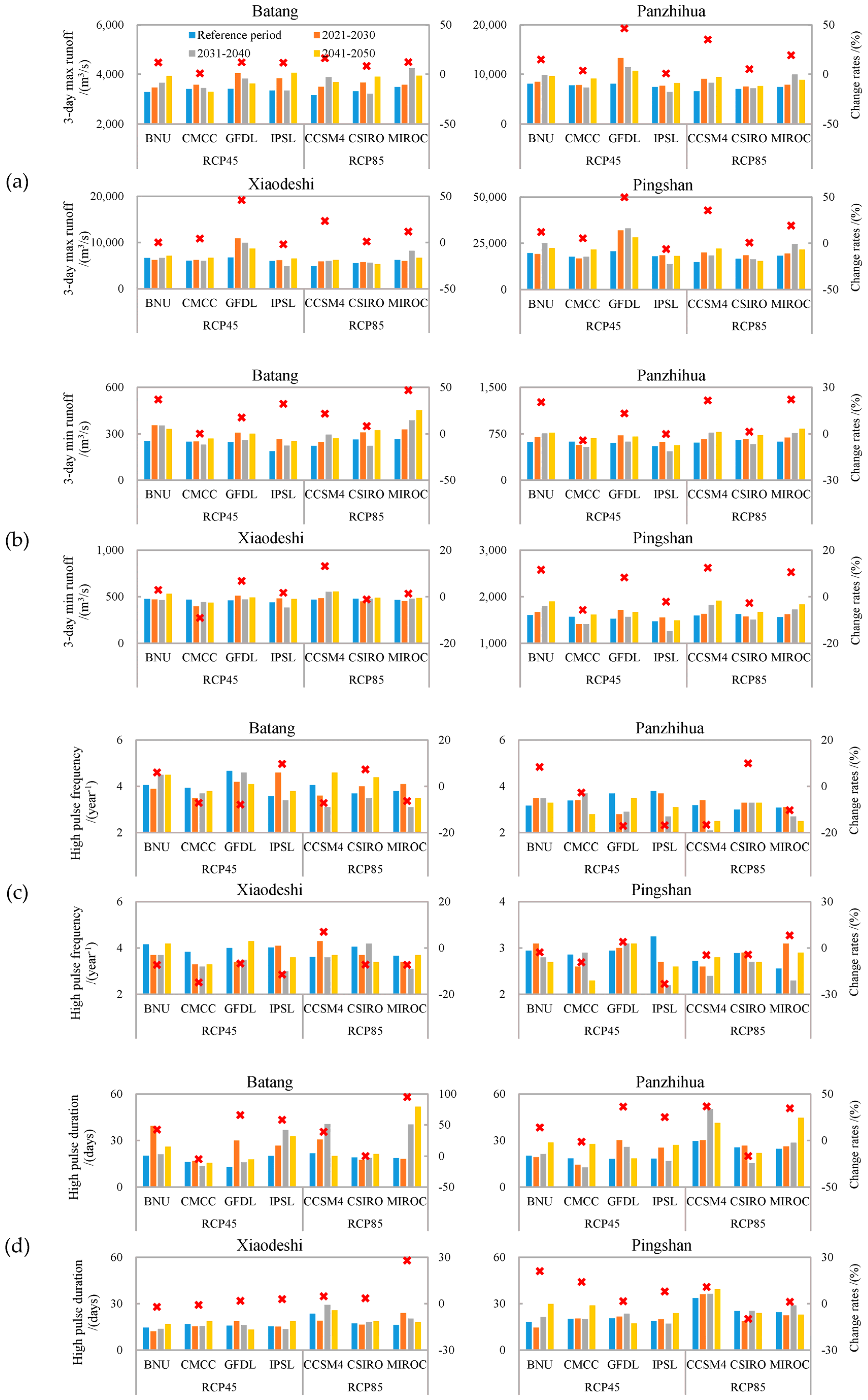
For the reason that the impact of land-use change is almost negligible in the Jinsha River Basin, therefore, in the latter part of the study the main focus is drawn on the runoff response in the context of climate change. The runoff simulations at the four hydrological stations in the Jinsha River Basin from 1970 to 2050 are obtained by combining the GCM projections with the SWAT model. In this research, respectively four and three typical GCMs from CMIP5 under RCP4.5 and RCP8.5 emission scenarios are selected (Table 8) based on 10% and 90% quantiles of the changes in precipitation dP (%) and temperature dT (°C). Taking 1970–2005 as the reference period, the changes in runoff extremes for the next three foresight periods (2021–2030, 2031–2040 and 2041–2050) are predicted, as shown in Figure 11. The abscissas and ordinates separately represent the typical GCMs under the two emission scenarios and the indicators of hydrological extremes, and the four pillars in different colors respectively stand for the reference period and the three foresight periods mentioned above. The variation trends of extreme runoff indicators compared with the reference period can be reflected in the figure.

It can be seen from Figure 11 that significant differences exist in the variation trends of runoff extremes at the same hydrological station predicted by different typical GCMs. Taking the indicator of 3-day max runoff at Batang station as an example, there are three variation modes: continuous increase (RCP4.5-BNU), increase first and then decrease (RCP4.5-CMCC/GFDL, RCP8.5-CCSM4/MIROC), and increase first, then decrease and then increase (RCP4.5-IPSL and RCP8.5-CSIRO), indicating large uncertainties in the prediction results of different GCMs. Therefore, from the statistical point of view, we should comprehensively take into consideration the results from multiple GCMs, and try to draw common conclusions which can serve as references for decision-makers. Seen from Figure 11a, almost all typical GCMs predict higher 3-day max runoff in the whole foresight period (2021–2050) compared with the reference period. The increasing rates vary from 0.9% to 50.2%, with the exception of RCP4.5-IPSL, which predicts slightly lower values at Xiaodeshi and Pingshan stations (−6.1%–−2.1%). Therefore, it can be inferred with high confidence that the 3-day max runoff in the Jinsha River Basin will increase in the near future. For the indicator of 3-day min runoff, the prediction results are generally higher in the future (2021–2050) compared with the reference period, with the changing rates varying from −9.1% to 47.0%. Regarding the characteristics of high pulse events, most typical GCMs predict decreased frequency and increased durations compared with the reference period.

In conclusion, the extreme runoff values (3-day max & min runoff in this paper) will probably increase compared with the reference period (1970–2005), indicating respectively rising and decreasing risks of extreme high and low flows in the Jinsha River Basin in the near future (2021–2050). Besides, the high pulse events will occur less frequently but last longer.

5. Conclusions

In this research, the trends and variations of extreme hydro-meteorological elements (precipitation, temperature and runoff) as well as the land-use changes in the Jinsha River Basin have been thoroughly investigated during the historical period. The SWAT model is employed to simulate the effects of land-use change and climate change on hydrological extremes using the method of scenarios simulation. In addition, the evolutions of various extreme runoff indicators are predicted by incorporating the climate simulations of seven typical GCMs from CMIP5. The conclusions are as follows:

• During the period of 1960–2017, generally insignificant rising trends in the intensity and frequency of extreme precipitation, statistically significant increasing trends in temperature, and the respectively insignificant rising and declining trends in the indicators of flood days (DH) and dry days (DK), have been identified in the Jinsha River Basin using the Mann–Kendall and CSD trend test methods. The above results reflect a fact that the risk of floods has generally increased, while the risk of droughts has declined in this period. As for the land-use data, the areas of building land and water body in the basin have changed greatly during 1980–2015. However, they occupy a very small proportion of the whole basin area.
• The good performance of SWAT model is confirmed with the multi-stations averaged NS values achieving 0.85 and PBIAS within 10% both in the calibration and verification period. Regarding the runoff extremes, the SWAT model has a better simulation effect on high flows compared with low flows.
• Seven typical GCMs are selected and the performance of GCM data in runoff simulations is evaluated by comparing SWAT simulations using historical downscaled GCM data with the SWAT simulations using climate observations in 1970–2005. Results show that the downscaled GCM data can well simulate the mean values of runoff, and acceptable simulation effects are achieved for the other extreme runoff indicators except for the frequency and duration of floods and extreme low flows.
• In this research, four extreme runoff indicators (3-day max and min runoff, high pulse frequency and duration) at four hydrological stations (Batang, Panzhihua, Xiaodeshi and Pingshan) are adopted to analyze the hydrological extremes in the Jinsha River Basin. The attribution analysis leads to the conclusion that the land-use change exerts little impact on runoff extremes during 1970–2017, possibly due to the relatively small extent of changes in land use. In contrast, the climate change is one of the dominant factors contributing to changes in hydrological extremes.
• By integrating the downscaled GCM data with the SWAT model, the trends and variations of hydrological extremes during 2021–2050 are predicted, with 1970–2005 used as reference period. Results indicate that both the indicators of 3-day max and 3-day min runoff will probably increase, and the high pulse events will occur less frequently but last longer in the near future.

The research improves our knowledge and understanding of the impacts of climate change and land-use change on hydrological extremes, and can provide references for the prevention of hydro-meteorological disasters as well as water resources management in the basin.

References

- Zhang, M.; Liu, N.; Harper, R.; Li, Q.; Liu, K.; Wei, X.; Ning, D.; Hou, Y.; Liu, S. A global review on hydrological responses to forest change across multiple spatial scales: Importance of scale, climate, forest type and hydrological regime. J. Hydrol. 2017, 546, 44–59. [Google Scholar] [CrossRef]
- Gao, G.; Fu, B.; Wang, S.; Liang, W.; Jiang, X. Determining the hydrological responses to climate variability and land use/cover change in the Loess Plateau with the Budyko framework. Sci. Total Environ. 2016, 557, 331–342. [Google Scholar] [CrossRef] [PubMed]
- Jarsjö, J.; Asokan, S.M.; Prieto, C.; Bring, A.; Destouni, G. Hydrological responses to climate change conditioned by historic alterations of land-use and water-use. Hydrol. Earth Syst. Sci. 2012, 16, 1335–1347. [Google Scholar] [CrossRef] [Green Version]
- Li, Z.; Liu, W.-Z.; Zhang, X.-C.; Zheng, F.-L. Impacts of land use change and climate variability on hydrology in an agricultural catchment on the Loess Plateau of China. J. Hydrol. 2009, 377, 35–42. [Google Scholar] [CrossRef]
- Liu, Z.; Yao, Z.; Huang, H.; Wu, S.; Liu, G. Land use and climate changes and their impacts on runoff in the Yarlung Zangbo river basin, China. Land Degrad. Dev. 2014, 25, 203–215. [Google Scholar] [CrossRef]
- Pan, S.; Liu, D.; Wang, Z.; Zhao, Q.; Zou, H.; Hou, Y.; Liu, P.; Xiong, L. Runoff responses to climate and land use/cover changes under future scenarios. Water 2017, 9, 475. [Google Scholar] [CrossRef]
- Yin, J.; He, F.; Xiong, Y.J.; Qiu, G.Y. Effects of land use/land cover and climate changes on surface runoff in a semi-humid and semi-arid transition zone in northwest China. Hydrol. Earth Syst. Sci. 2017, 21, 183–196. [Google Scholar] [CrossRef] [Green Version]
- Burn, D.H.; Sharif, M.; Zhang, K. Detection of trends in hydrological extremes for Canadian watersheds. Hydrol. Process. 2010, 24, 1781–1790. [Google Scholar] [CrossRef]
- Taye, M.T.; Ntegeka, V.; Ogiramoi, N.; Willems, P. Assessment of climate change impact on hydrological extremes in two source regions of the Nile River Basin. Hydrol. Earth Syst. Sci. 2011, 15, 209–222. [Google Scholar] [CrossRef] [Green Version]
- Hoang, L.P.; Lauri, H.; Kummu, M.; Koponen, J.; van Vliet, M.; Supit, I.; Leemans, R.; Kabat, P.; Ludwig, F. Mekong River flow and hydrological extremes under climate change. Hydrol. Earth Syst. Sci. 2016, 20, 3027–3041. [Google Scholar] [CrossRef] [Green Version]
- Wu, P.; Christidis, N.; Stott, P. Anthropogenic impact on Earth’s hydrological cycle. Nat. Clim. Chang. 2013, 3, 807. [Google Scholar] [CrossRef]
- Allen, M.R.; Ingram, W.J. Constraints on future changes in climate and the hydrologic cycle. Nature 2002, 419, 224. [Google Scholar] [CrossRef] [PubMed]
- Donat, M.G.; Lowry, A.L.; Alexander, L.V.; O’Gorman, P.A.; Maher, N. More extreme precipitation in the world’s dry and wet regions. Nat. Clim. Chang. 2016, 6, 508. [Google Scholar] [CrossRef]
- Trenberth, K.E. Changes in precipitation with climate change. Clim. Res. 2011, 47, 123–138. [Google Scholar] [CrossRef] [Green Version]
- Alexander, L.; Zhang, X.; Peterson, T.; Caesar, J.; Gleason, B.; Klein Tank, A.; Haylock, M.; Collins, D.; Trewin, B.; Rahimzadeh, F. Global observed changes in daily climate extremes of temperature and precipitation. J. Geophys. Res. Atmos. 2006, 111. [Google Scholar] [CrossRef] [Green Version]
- Westra, S.; Alexander, L.V.; Zwiers, F.W. Global increasing trends in annual maximum daily precipitation. J. Clim. 2013, 26, 3904–3918. [Google Scholar] [CrossRef]
- Min, S.-K.; Zhang, X.; Zwiers, F.W.; Hegerl, G.C. Human contribution to more-intense precipitation extremes. Nature 2011, 470, 378. [Google Scholar] [CrossRef] [PubMed]
- Kharin, V.V.; Zwiers, F.; Zhang, X.; Wehner, M. Changes in temperature and precipitation extremes in the CMIP5 ensemble. Clim. Chang. 2013, 119, 345–357. [Google Scholar] [CrossRef]
- Sillmann, J.; Kharin, V.; Zwiers, F.; Zhang, X.; Bronaugh, D. Climate extremes indices in the CMIP5 multimodel ensemble: Part 2. Future climate projections. J. Geophys. Res. Atmos. 2013, 118, 2473–2493. [Google Scholar] [CrossRef]
- Field, C.B.; Barros, V.; Stocker, T.; Qin, D.; Dokken, D.; Ebi, K.; Mastrandrea, M.; Mach, K.; Plattner, G.; Allen, S. IPCC, 2012: Managing the Risks of Extreme Events and Disasters to Advance Climate Change Adaptation. A Special Report of Working Groups I and II of the Intergovernmental Panel on Climate Change; Cambridge University Press: Cambridge, UK; New York, NY, USA, 2012; Volume 30, pp. 7575–7613. [Google Scholar]
- Madsen, H.; Lawrence, D.; Lang, M.; Martinkova, M.; Kjeldsen, T. Review of trend analysis and climate change projections of extreme precipitation and floods in Europe. J. Hydrol. 2014, 519, 3634–3650. [Google Scholar] [CrossRef] [Green Version]
- Welde, K.; Gebremariam, B. Effect of land use land cover dynamics on hydrological response of watershed: Case study of Tekeze Dam watershed, northern Ethiopia. Int. Soil Water Conserv. Res. 2017, 5, 1–16. [Google Scholar] [CrossRef]
- Wang, H.; Sun, F.; Xia, J.; Liu, W. Impact of LUCC on streamflow based on the SWAT model over the Wei River basin on the Loess Plateau in China. Hydrol. Earth Syst. Sci. 2017, 21, 1929. [Google Scholar] [CrossRef]
- Lin, B.; Chen, X.; Yao, H.; Chen, Y.; Liu, M.; Gao, L.; James, A. Analyses of landuse change impacts on catchment runoff using different time indicators based on SWAT model. Ecol. Indic. 2015, 58, 55–63. [Google Scholar] [CrossRef]
- Nie, W.; Yuan, Y.; Kepner, W.; Nash, M.S.; Jackson, M.; Erickson, C. Assessing impacts of Landuse and Landcover changes on hydrology for the upper San Pedro watershed. J. Hydrol. 2011, 407, 105–114. [Google Scholar] [CrossRef]
- Sanyal, J.; Densmore, A.L.; Carbonneau, P. Analysing the effect of land-use/cover changes at sub-catchment levels on downstream flood peaks: A semi-distributed modelling approach with sparse data. Catena 2014, 118, 28–40. [Google Scholar] [CrossRef] [Green Version]
- Wan, R.; Yang, G. Influence of land use/cover change on storm runoff—A case study of Xitiaoxi River Basin in upstream of Taihu Lake Watershed. Chin. Geogr. Sci. 2007, 17, 349–356. (in Chinese). [Google Scholar] [CrossRef]
- O’Donnell, G.; Ewen, J.; O’Connell, P. Sensitivity maps for impacts of land management on an extreme flood in the Hodder catchment, UK. Phys. Chem. Earth Parts A/B/C 2011, 36, 630–637. [Google Scholar] [CrossRef]
- Chen, Y.; Xu, Y.; Yin, Y. Impacts of land use change scenarios on storm-runoff generation in Xitiaoxi basin, China. Quat. Int. 2009, 208, 121–128. [Google Scholar] [CrossRef]
- Ali, M.; Khan, S.J.; Aslam, I.; Khan, Z. Simulation of the impacts of land-use change on surface runoff of Lai Nullah Basin in Islamabad, Pakistan. Landsc. Urban Plan. 2011, 102, 271–279. [Google Scholar] [CrossRef]
- El-Khoury, A.; Seidou, O.; Lapen, D.; Que, Z.; Mohammadian, M.; Sunohara, M.; Bahram, D. Combined impacts of future climate and land use changes on discharge, nitrogen and phosphorus loads for a Canadian river basin. J. Environ. Manag. 2015, 151, 76–86. [Google Scholar] [CrossRef] [Green Version]
- Zhang, L.; Karthikeyan, R.; Bai, Z.; Srinivasan, R. Analysis of streamflow responses to climate variability and land use change in the Loess Plateau region of China. Catena 2017, 154, 1–11. [Google Scholar] [CrossRef]
- Tan, M.L.; Ibrahim, A.L.; Yusop, Z.; Duan, Z.; Ling, L. Impacts of land-use and climate variability on hydrological components in the Johor River basin, Malaysia. Hydrol. Sci. J. 2015, 60, 873–889. [Google Scholar] [CrossRef]
- Zhang, X.; Zhang, L.; Zhao, J.; Rustomji, P.; Hairsine, P. Responses of streamflow to changes in climate and land use/cover in the Loess Plateau, China. Water Resour. Res. 2008, 44. [Google Scholar] [CrossRef]
- Leng, G.; Tang, Q.; Rayburg, S. Climate change impacts on meteorological, agricultural and hydrological droughts in China. Glob. Planet. Chang. 2015, 126, 23–34. [Google Scholar] [CrossRef]
- Apurv, T.; Mehrotra, R.; Sharma, A.; Goyal, M.K.; Dutta, S. Impact of climate change on floods in the Brahmaputra basin using CMIP5 decadal predictions. J. Hydrol. 2015, 527, 281–291. [Google Scholar] [CrossRef]
- Wu, C.; Huang, G.; Yu, H. Prediction of extreme floods based on CMIP5 climate models: A case study in the Beijiang River basin, South China. Hydrol. Earth Syst. Sci. 2015, 19, 1385–1399. [Google Scholar] [CrossRef]
- Romanowicz, R.J.; Bogdanowicz, E.; Debele, S.E.; Doroszkiewicz, J.; Hisdal, H.; Lawrence, D.; Meresa, H.K.; Napiórkowski, J.J.; Osuch, M.; Strupczewski, W.G. Climate change impact on hydrological extremes: Preliminary results from the Polish-Norwegian Project. Acta Geophys. 2016, 64, 477–509. [Google Scholar] [CrossRef]
- Jia, H.J.; Wan, R.R. Simulating the impacts of land use/cover change on storm-runoff for a mesoscale watershed in east China. Adv. Mater. Res. 2011, 347–353, 3856–3862. [Google Scholar] [CrossRef]
- Miller, J.D.; Hess, T. Urbanisation impacts on storm runoff along a rural-urban gradient. J. Hydrol. 2017, 552, 474–489. [Google Scholar] [CrossRef]
- Schilling, K.E.; Gassman, P.W.; Kling, C.L.; Campbell, T.; Jha, M.K.; Wolter, C.F.; Arnold, J.G. The potential for agricultural land use change to reduce flood risk in a large watershed. Hydrol. Process. 2014, 28, 3314–3325. [Google Scholar] [CrossRef]
- Jothityangkoon, C.; Hirunteeyakul, C.; Boonrawd, K.; Sivapalan, M. Assessing the impact of climate and land use changes on extreme floods in a large tropical catchment. J. Hydrol. 2013, 490, 88–105. [Google Scholar] [CrossRef]
- Graham, W.J. Should dams be modified for the probable maximum flood? J. Am. Water Resour. Assoc. 2000, 36, 953–963. [Google Scholar] [CrossRef]
- Najafi, M.R.; Moradkhani, H. Multi-model ensemble analysis of runoff extremes for climate change impact assessments. J. Hydrol. 2015, 525, 352–361. [Google Scholar] [CrossRef] [Green Version]
- Chiew, F.; Teng, J.; Vaze, J.; Post, D.; Perraud, J.; Kirono, D.; Viney, N. Estimating climate change impact on runoff across southeast Australia: Method, results, and implications of the modeling method. Water Resour. Res. 2009, 45. [Google Scholar] [CrossRef]
- Najafi, M.; Moradkhani, H. A hierarchical Bayesian approach for the analysis of climate change impact on runoff extremes. Hydrol. Process. 2014, 28, 6292–6308. [Google Scholar] [CrossRef]
- Liu, X.; Peng, D.; Xu, Z. Identification of the Impacts of Climate Changes and Human Activities on Runoff in the Jinsha River Basin, China. Adv. Meteorol. 2017, 2017, 9. [Google Scholar] [CrossRef]
- Abbaspour, K.C.; Yang, J.; Maximov, I.; Siber, R.; Bogner, K.; Mieleitner, J.; Zobrist, J.; Srinivasan, R. Modelling hydrology and water quality in the pre-alpine/alpine Thur watershed using SWAT. J. Hydrol. 2007, 333, 413–430. [Google Scholar] [CrossRef]
- Meng, X.; Wang, H.; Lei, X.; Cai, S.; Wu, H.; Ji, X.; Wang, J. Hydrological modeling in the Manas River Basin using soil and water assessment tool driven by CMADS. Teh. Vjesn. 2017, 24, 525–534. [Google Scholar]
- Martínez-Casasnovas, J.A.; Ramos, M.C.; Benites, G. Soil and Water Assessment Tool Soil Loss Simulation at the Sub-Basin Scale in the Alt Penedès–Anoia Vineyard Region (Ne Spain) in the 2000s. Land Degrad. Dev. 2016, 27, 160–170. [Google Scholar] [CrossRef]
- Teshager, A.D.; Gassman, P.W.; Secchi, S.; Schoof, J.T.; Misgna, G. Modeling agricultural watersheds with the soil and water assessment tool (swat): Calibration and validation with a novel procedure for spatially explicit hrus. Environ. Manag. 2016, 57, 894–911. [Google Scholar] [CrossRef]
- Gassman, P.W.; Reyes, M.R.; Green, C.H.; Arnold, J.G. The soil and water assessment tool: Historical development, applications, and future research directions. Trans. ASABE 2007, 50, 1211–1250. [Google Scholar] [CrossRef]
- Neitsch, S.L.; Arnold, J.G.; Kiniry, J.R.; Williams, J.R. Soil and Water Assessment Tool Theoretical Documentation Version 2009; Texas Water Resources Institute: College Station, TX, USA, 2011. [Google Scholar]
- Penman, H.L. Natural evaporation from open water, bare soil and grass. Proc. R. Soc. Lond. Ser. A Math. Phys. Sci. 1948, 193, 120–145. [Google Scholar] [Green Version]
- Monteith, J.L. Evaporation and environment, in the state and movement of water in living organisms. Symp. Soc. Exp. Biol. 1965, 19, 205–234. [Google Scholar] [PubMed]
- USDA-SCS. National Engineering Hanbook, Section 4–Hydrology; US Government Printing Office: Washington, DC, USA, 1972.
- Chow, V.T. Handbook of Applied Hydrology; McGraw-Hill Book Company: New York, NY, USA, 1964. [Google Scholar]
- Mann, H.B. Nonparametric Tests Against Trend; The Econometric Society: Cleveland, OH, USA, 1945; pp. 245–259. [Google Scholar]
- Kendall, M.G. Rank Correlation Methods, 4th ed.; Charles Griffin: London, UK, 1975. [Google Scholar]
- Hirsch, R.M.; Slack, J.R. A nonparametric trend test for seasonal data with serial dependence. Water Resour. Res. 1984, 20, 727–732. [Google Scholar] [CrossRef]
- Onyutha, C. Identification of sub-trends from hydro-meteorological series. Stoch. Environ. Res. Risk Assess. 2016, 30, 189–205. [Google Scholar] [CrossRef]
- Onyutha, C. On rigorous drought assessment using daily time scale: Non-stationary frequency analyses, revisited concepts, and a new method to yield non-parametric indices. Hydrology 2017, 4, 48. [Google Scholar] [CrossRef]
- Onyutha, C. Statistical uncertainty in hydrometeorological trend analyses. Adv. Meteorol. 2016, 2016, 26. [Google Scholar] [CrossRef]
- Onyutha, C. Statistical analyses of potential evapotranspiration changes over the period 1930–2012 in the Nile River riparian countries. Agric. For. Meteorol. 2016, 226, 80–95. [Google Scholar] [CrossRef]
- Richter, B.; Thomas, G. Restoring environmental flows by modifying dam operations. Ecol. Soc. 2007, 12, 12. [Google Scholar] [CrossRef]
- Richter, B.D.; Mathews, R.; Harrison, D.L.; Wigington, R. Ecologically sustainable water management: Managing river flows for ecological integrity. Ecol. Appl. 2003, 13, 206–224. [Google Scholar] [CrossRef]
- Richter, B.D.; Baumgartner, J.V.; Powell, J.; Braun, D.P. A method for assessing hydrologic alteration within ecosystems. Conserv. Biol. 1996, 10, 1163–1174. [Google Scholar] [CrossRef]
- Conservancy, N. Indicators of Hydrologic Alteration Version 7.1: User’s Manual; The Nature Conservancy: Arlington County, VA, USA, 2009. [Google Scholar]
- Kusangaya, S.; Toucher, M.L.W.; van Garderen, E.A. Evaluation of uncertainty in capturing the spatial variability and magnitudes of extreme hydrological events for the uMngeni catchment, South Africa. J. Hydrol. 2018, 557, 931–946. [Google Scholar] [CrossRef]
- Saraiva Okello, A.; Masih, I.; Uhlenbrook, S.; Jewitt, G.; Van der Zaag, P.; Riddell, E. Drivers of spatial and temporal variability of streamflow in the Incomati River basin. Hydrol. Earth Syst. Sci. 2015, 19, 657–673. [Google Scholar] [CrossRef] [Green Version]
- Gao, Y.; Vogel, R.M.; Kroll, C.N.; Poff, N.L.; Olden, J.D. Development of representative indicators of hydrologic alteration. J. Hydrol. 2009, 374, 136–147. [Google Scholar] [CrossRef]
- Yang, T.; Zhang, Q.; Chen, Y.D.; Tao, X.; Xu, C.Y.; Chen, X. A spatial assessment of hydrologic alteration caused by dam construction in the middle and lower Yellow River, China. Hydrol. Process. Int. J. 2008, 22, 3829–3843. [Google Scholar] [CrossRef]
- Chen, J.; Brissette, F.P.; Chaumont, D.; Braun, M. Performance and uncertainty evaluation of empirical downscaling methods in quantifying the climate change impacts on hydrology over two North American river basins. J. Hydrol. 2013, 479, 200–214. [Google Scholar] [CrossRef]
- Chen, J.; Brissette, F.P.; Leconte, R. Uncertainty of downscaling method in quantifying the impact of climate change on hydrology. J. Hydrol. 2011, 401, 190–202. [Google Scholar] [CrossRef]
- Shahbeik, S.; Afzal, P.; Moarefvand, P.; Qumarsy, M. Comparison between ordinary kriging (OK) and inverse distance weighted (IDW) based on estimation error. Case study: Dardevey iron ore deposit, NE Iran. Arab. J. Geosci. 2014, 7, 3693–3704. [Google Scholar] [CrossRef]
- Chen, F.-W.; Liu, C.-W. Estimation of the spatial rainfall distribution using inverse distance weighting (IDW) in the middle of Taiwan. Paddy Water Environ. 2012, 10, 209–222. [Google Scholar] [CrossRef]
- Chen, Q.H.; Zhang, J.; Hou, Y.K.; Shen, M.X.; Chen, J.; Xu, C.Y. Impacts of climate change and LUCC on runoff of Jinsha River Basin in recent 60 years (in Chinese). Yangtze River 2018, 49, 47–53. [Google Scholar]
- Immerzeel, W.; Pellicciotti, F.; Bierkens, M. Rising river flows throughout the twenty-first century in two Himalayan glacierized watersheds. Nat. Geosci. 2013, 6, 742. [Google Scholar] [CrossRef]
Figure 1.
Map of the Jinsha River Basin showing the location of weather stations, hydrological stations, reaches and digital elevation model (DEM).
Figure 2.
The land-use distribution in the Jinsha River Basin measured in 1980.
Figure 3.
Spatial distribution of mean (a), Mann–Kendall (M–K) test Z values (b) and cumulative sum of rank difference (CSD) test Z values (c) of annual maximum 1-day precipitation in the Jinsha River Basin during 1960–2017.
Figure 4.
Spatial distribution of extreme precipitation thresholds (a), M–K test Z values (b) and CSD test Z values (c) of extreme precipitation frequency in the Jinsha River Basin during 1960–2017.
Figure 5.
Spatial distribution of the annual averaged temperature (a) and the inter-annual variation of maximum, minimum and average temperature (b) in the Jinsha River Basin during 1960–2017.
Figure 6.
Temporal variations of the four extreme runoff indicators in the Jinsha River Basin during 1960–2017 in Zhimenda (a), Batang (b), Shigu (c), Yajiang (d), Luning (e), Xiaodeshi (f), Panzhihua (g), Huatan (h) and Pingshan stations (i), which are moving on average every 5 years.
Figure 7.
Deviation factors (DF) of 18 extreme runoff indicators of simulated runoff compared with observed runoff at nine hydrological stations in the Jinsha River Basin during the calibration and verification periods (1970–2008).
Figure 8.
Schematic diagram of the selection of typical general circulation models (GCMs) under RCP4.5 emission scenario.
Figure 9.
Deviation factors (DF) of 18 extreme runoff indicators of SWAT simulations using historical GCM data (1970–2005) compared with SWAT simulations using historical climate instrumentations (1970–2005) in the Jinsha River Basin.
Figure 10.
The magnitudes of four extreme runoff indicators simulated by the SWAT model including annual 3-day max runoff (a), 3-day min runoff (b), high pulse frequency (c) and high pulse duration (d) under 16 scenarios at four hydrological stations in the Jinsha River Basin.
Figure 11.
Evolution of four extreme hydrological indicators in Jinsha River Basin, including 3-day max runoff (a), 3-day min runoff (b), high pulse frequency (c) and high pulse duration (d), from the reference period (1970–2005) to the three foresight periods (2021–2030, 2031–2040, 2041–2050). The red points represent the averaged percent changes of hydrological indicators in the whole foresight period (2021–2050) compared with the reference period. All of the sub-figures share the same legend as Batang station in sub-figure (a).