1. Introduction
Desalination of alternative waters, such as brackish water, seawater, municipal, and industrial wastewater, has become a critical strategy to expand traditional water supplies and to alleviate water shortages [
1]. Electrodialysis (ED) is a membrane desalination technology that uses semi-permeable ion-exchange membranes (IEMs) to selectively separate salt ions in water under the influence of an electric field [
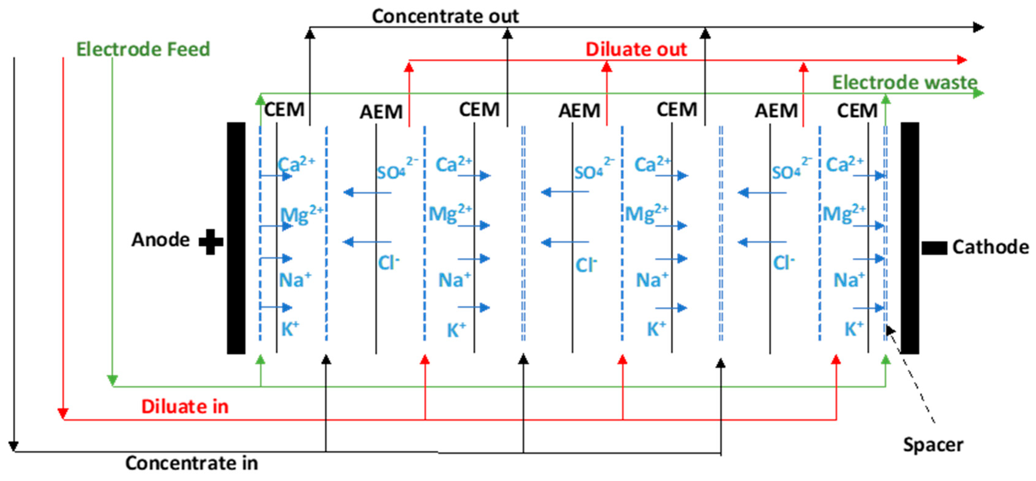
2]. An ED stack consists of pairs of anion-exchange membranes (AEMs) and cation-exchange membranes (CEMs) arranged alternatingly between an anode and a cathode (
Figure 1). The positively charged cations migrate toward the cathode, pass the negatively charged CEM, and are rejected by the positively charged AEM. The opposite occurs when the negatively charged anions migrate toward the anode. This results in an alternatively increasing ion concentration in one compartment (concentrate) and decreasing salt concentration in the other (diluate). The process can be viewed as a dialysis process, where the ion diffusion across the membranes is amplified and orientated by an electric field. Electrodialysis reversal (EDR) is a modified ED process, where the electrical polarity of the electrodes is reversed periodically. This results in a reversal in the direction of the ion transport so that the concentrated stream becomes the diluate stream and vice versa. This self-flushing of scale forming ions and fouling matter in concentrate compartments allows EDR to operate at a higher water recovery than ED.
Electrodialysis and EDR have been utilized for decades to desalinate brackish water, treat municipal and industrial wastewater, and produce NaCl from seawater [
1]. It has also found applications in chemical processes, as well as the food, beverage, and drug industries. Despite the broad application of ED/EDR, the number of experiments and simulations concerned with the thermodynamics and fluid dynamics of the ED process is very limited [
3]. For example, a key parameter for the design and operation of ED is the limiting current density (LCD). It is typically identified as the diffusion-limited current density, corresponding to the complete solute depletion in the layer adjacent to the membrane surface [
2]. The limiting regime in ED is associated with the appearance of electroconvective structures near the membranes [
3]. The structures are caused by an electrokinetic instability (EKI). The phenomena involved in the limiting region are not yet fully understood. Any improvement of the effectiveness of the ED process based on a reduction of the energy losses (e.g., Chehayeb and Lienhard [
3]) and methods that overcome inherent operating limitations have strong implications for environmental sustainability and the water, food, and chemical industries.
This paper is concerned with the factors governing the onset of the overlimiting regime in ED. Of particular interest are the effects of the applied voltage, salt concentration, and membrane surface geometry on the onset of the EKI. Towards that end, simulations of the phenomena near a CEM were carried out for a binary electrolyte solution. Because the hydrodynamics and ion transport for CEMs and AEMs are similar, the present findings transfer over to AEMs. The paper starts out with a discussion of the onset of the overlimiting regime and how it is related to the EKI. This section is followed by a discussion of the governing equations, the setup of the simulations, and the defining parameters. Instantaneous visualizations and time histories of the current density are employed to investigate the onset of the EKI. The paper concludes with a brief discussion of the results and their relevance for ED.
2. Overlimiting Regime and Electrokinetic Instability
When the voltage is low enough, the cations in the diffusion layer are drawn to the CEM surface by both migration and diffusion. For the anions, the diffusive and electromigration fluxes cancel each other out. The solution remains locally charge neutral with the exception of a thin electric double layer (EDL) with a thickness of tens of micrometers that forms on the selective membrane surface. As the voltage and hence the concentration gradients are increased, the electroneutrality condition demands very small anion concentrations near the CEM surface. For some limiting voltage, the electroneutrality condition in the diffusion layer is violated and another layer emerges between the EDL and the diffusion layer, which is known as extended space charge layer. Beyond a critical voltage, an instability sets in (here referred to as electrokinetic instability, EKI) and disturbance amplification results in the formation of organized flow structures and electroconvection. The flow structures eject fluid and charge density away from the membrane and substantially increase the current density. For mono-valent binary solutions, the magnitude of the limiting current density is inversely proportional to the boundary layer thickness [
4]. The electroconvective structures are similar to those arising from the Rayleigh–Bénard instability, which is driven by opposing gravity and buoyancy forces.
Based on experiments, Rubinstein et al. [
5] made a connection between the onset of the overlimiting regime, which is associated with an unsteadiness of the current density, and the occurrence of the EKI. Later, simulations and stability investigations followed (e.g., Demekhin et al. [
6], Rubinstein and Zaltzman [
7,
8]). A review on electroconvective micro-structures and related phenomena was provided by Chang et al. [
9]. Despite the small length-scales associated with electroconvection, the instability can lead to broad spectra and an energy cascade similar to those observed in turbulent flows. Dye visualizations by Yossifon et al. [
10] revealed vortices with an initial wavelength of 10 to
(close to the thickness of the boundary layer). As the vortices grow in size they merge and the wavelength is reduced. For narrow microchannels, the channel height determines the final vortex size [
10]. When fully developed, the size of the structures is of the order of the distance between the membranes, which is typically less than
. For very narrow channels, the vortices never form, which, of course, suggests that the instability is suppressed.
The simulation of reverse osmosis (RO) and even more so ED processes is challenging because of the complex flow physics and the large spread of length-scales from nanometer-sized pores to millimeter-sized spacers. For liquids, the continuum assumption breaks down for length scales around
. Although some researchers argue that lattice Boltzmann methods should be employed to describe the flow in ED stacks (because of the small scales), the general consensus is that the continuous flow model (Navier–Stokes equations) is accurate enough. Aside from the Navier–Stokes (N–S) equations, for ED processes additional conservation equations for the molar concentrations,
, of the ions, the Nernst–Planck (N–P) equations, have to be solved. Diffusion and electromigration dominate the ionic transport in the boundary layer. Since the water flux through the IEMs in ED is typically insignificant, the convection terms are often neglected. For example, Kim et al. [
11] developed a mathematical model for the steady-state transport of three ion species through an ED cell based on diffusion and migration.
Research aimed at understanding the physics of the boundary layer near the IEMs has to consider the complete N–P equations. Druzgalski et al. [
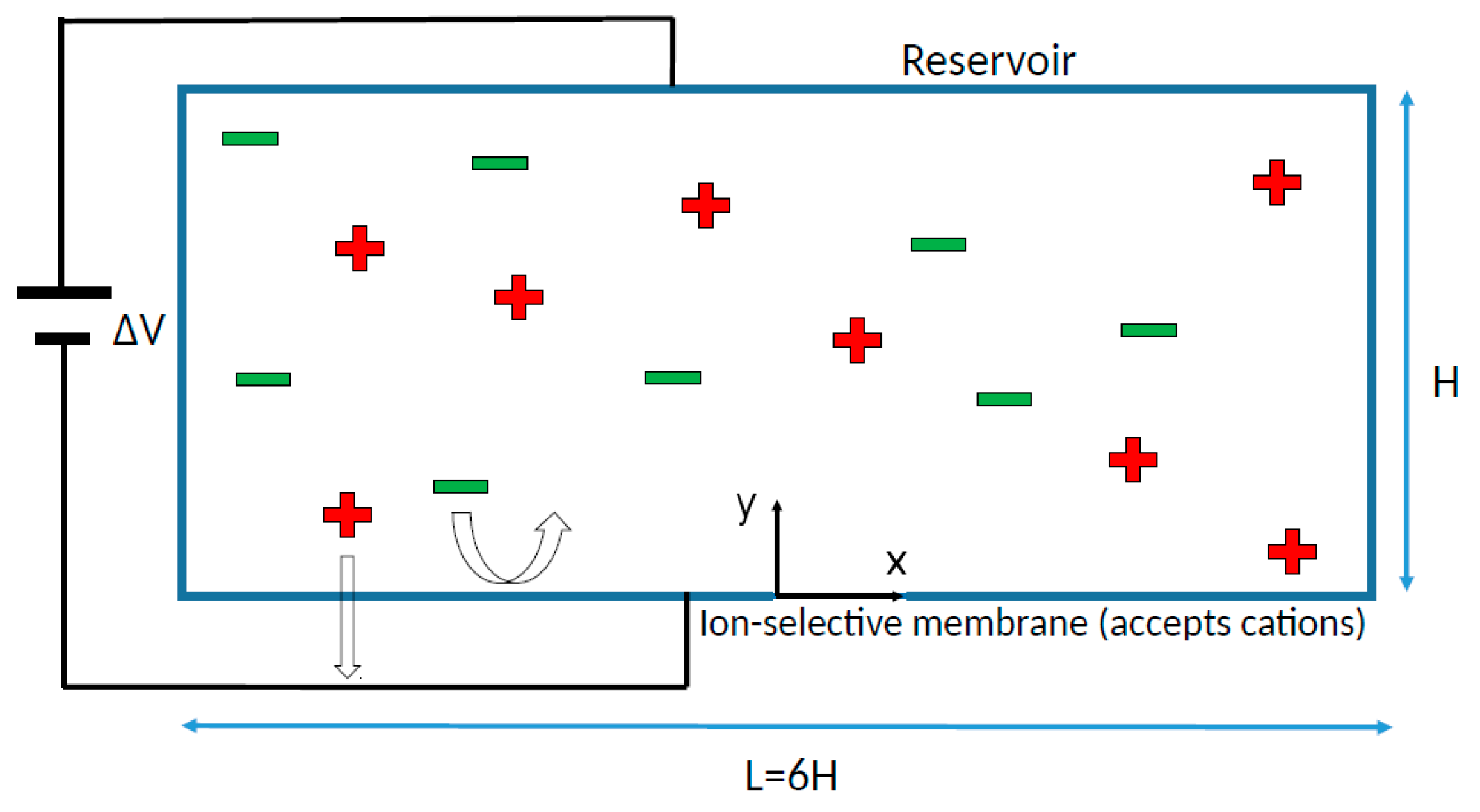
12] solved the coupled two-dimensional (2-D) N–P and N–S equations to investigate the EKI for a binary electrolyte between an IEM and a reservoir (water flow channel). They also presented a framework for the development of ensemble-averaged models (similar to Reynolds-averaged Navier–Stokes models) for the inclusion of the resulting electroconvective-driven mixing processes. Similar simulations were performed by Zourmand et al. [
13] and Enciso et al. [
14]. Enciso et al. [
14] performed experiments and found a 16% difference between the computed and measured mass transfer coefficients. Pimenta and Alves [
15] developed an OpenFOAM solver, rheoEFoam, which is part of the rheoTool suite, for the simulation of electrically-driven flows. Importance was placed on the conservation of the ionic species, numerical robustness, and an overall second-order-accuracy of the discretization. RheoEFoam was validated by comparison with the binary electrolyte problem by Druzgalski et al. [
12].
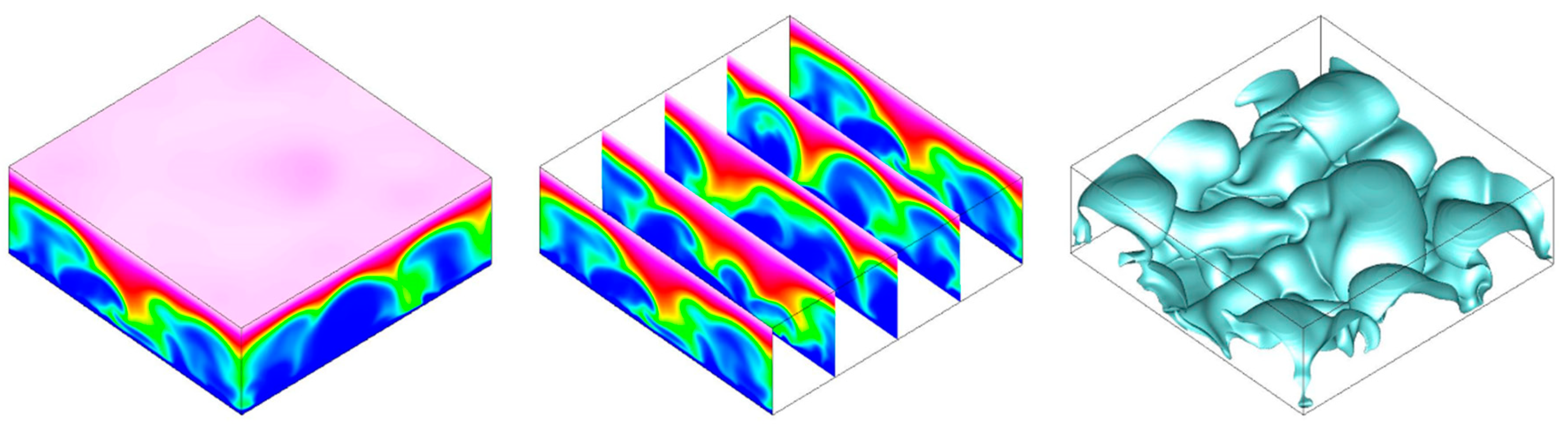
Demekhin et al. [
16] carried out three-dimensional (3-D) simulations of a reservoir-membrane configuration and found three typical flow structures arising from the EKI: Two-dimensional (2-D) counter-rotating rolls, regular hexagonal (“bee hive”) structures, and more chaotic 3-D structures. The onset of the instability and the type of the resulting flow structures were found to depend on the applied voltage and a coupling coefficient,
, between the hydrodynamics and the electrostatics. Here,
is the permittivity,
is the electric potential,
is the dynamic viscosity, and
is the ionic diffusivity. When the voltage exceeded a first critical value, counter-rotating rolls formed. When the voltage was increased further beyond a second critical value, hexagonal structures arose. Finally, for very large voltages, the flow became chaotic and the spectra filled up. Druzgalski and Mani [
17] employed 3-D simulations to investigate the fully chaotic regime. They found short-lived high-current-density spots that appeared randomly on the membrane surface and contributed significantly to the mean current density.
Rubinstein and Zaltzman [
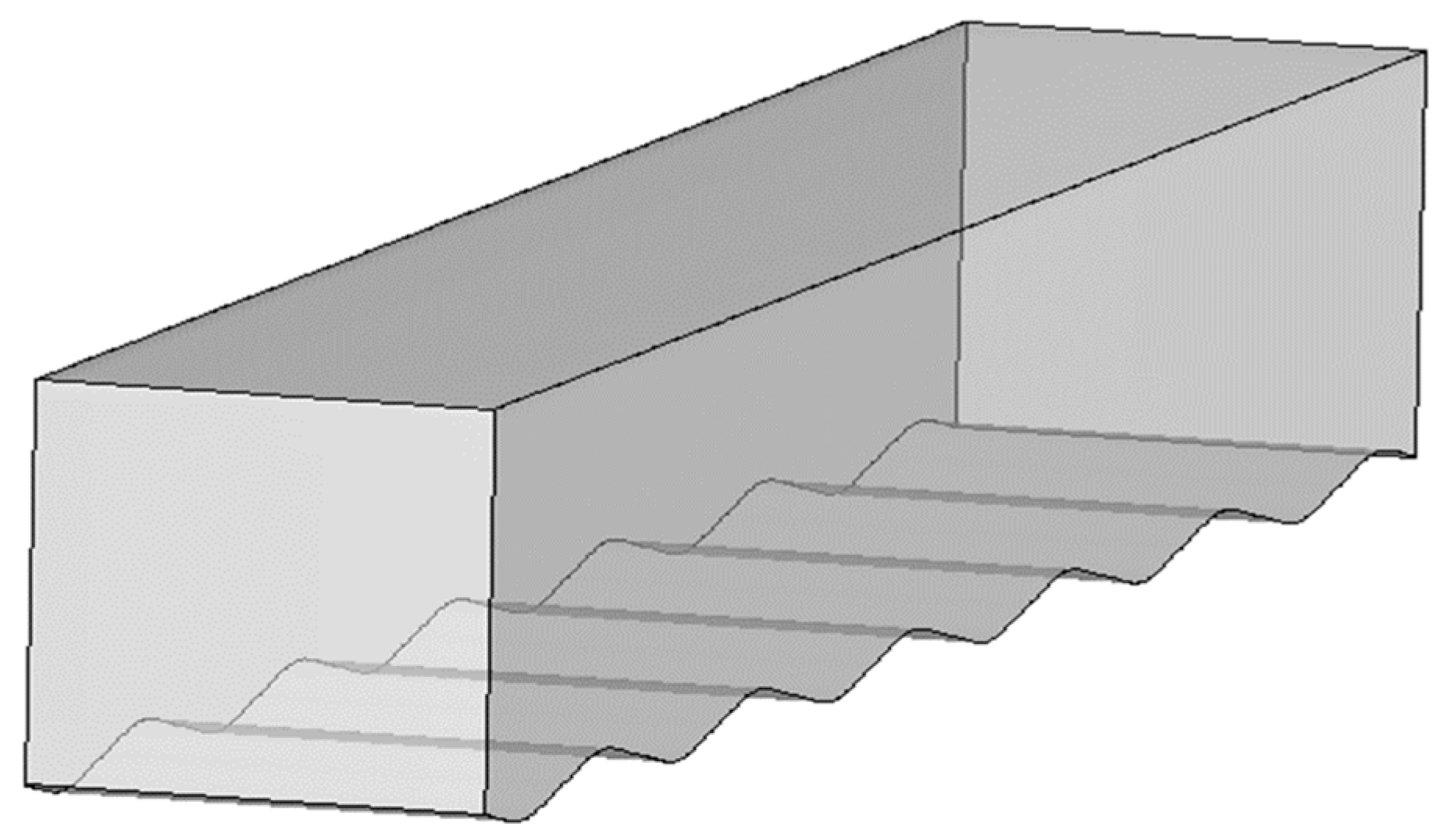
8] showed that the EKI leads to the growth of disturbances with a preferred natural wavelength whose initial amplitude can be increased by imparting a minute waviness on the membrane surface. This paper is concerned with the dependence of the current density on the wavelength of the waviness of the membrane surface. The present effort has been motivated by research in fluid dynamics that has shown that the growth of instability waves can be influenced. Saric et al. [
18] investigated crossflow transition on swept wings. By adding micro-sized roughness elements that were spaced at a wavelength below the most unstable (natural) wavelength of the instability, the growth rate of the steady crossflow mode could be reduced and transition to turbulence could be delayed. Embacher and Fasel [
19] stabilized a secondary instability by forcing the primary instability at a wavelength that was incommensurate with the most amplified natural wavelength. Finally, streamwise riblets with a spanwise wavelength close to the wavelength of the naturally occurring near-wall streaks in turbulent boundary layers (the wavelength can be as small as
) were found to reduce the turbulent skin-friction drag [
20].
This paper shows that by transferring these ideas to ED applications, the onset of the EKI and the overlimiting regime can be delayed. Of particular relevance for the present investigations are the results for wavy membranes by Rubinstein and Zaltzman [
8] and the crossflow instability research by Saric et al. [
18]. As will be shown later, the required dimensions of the membrane surface structures will be much smaller than what has already been considered in the literature (e.g., Güler et al. [
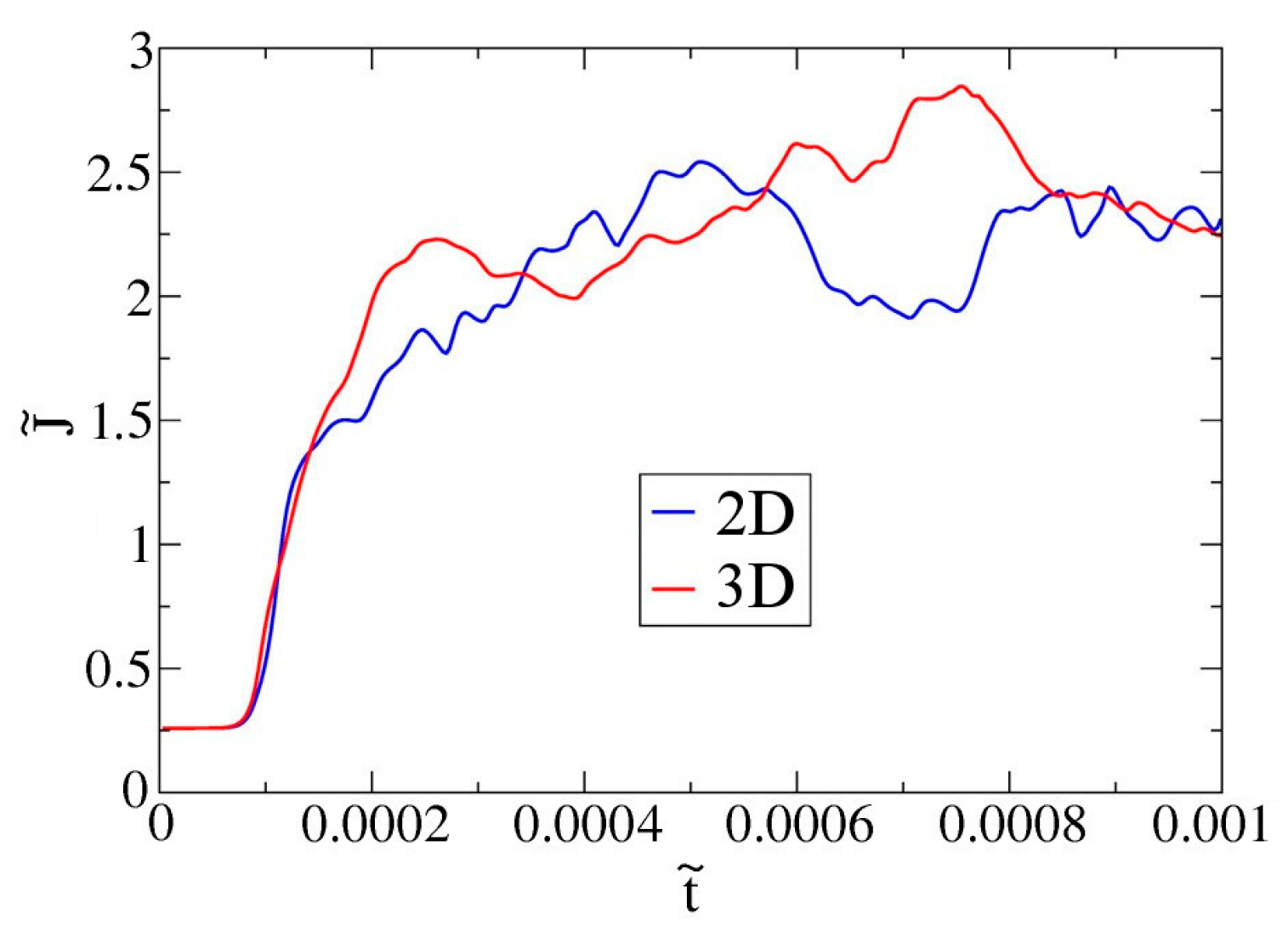
21]). All of the present simulations were carried out with the rheoEFoam code, which was developed by Pimenta and Alves [
15]. The majority of the simulations are 2-D. The concentration and the strength of the electric field were varied. For one case, a 3-D simulation was carried out to demonstrate the relevance of the 2-D simulations.
5. Discussion
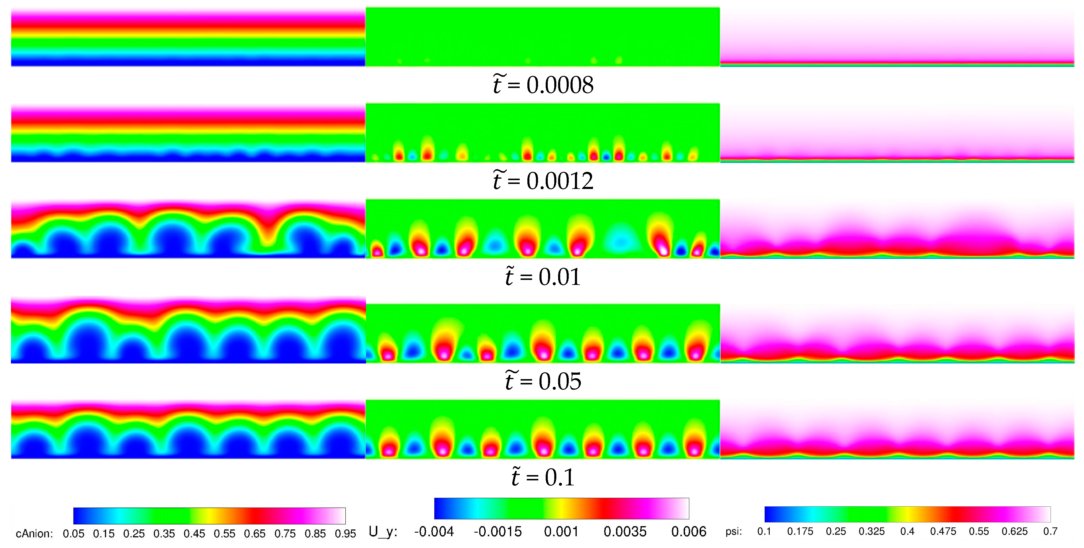
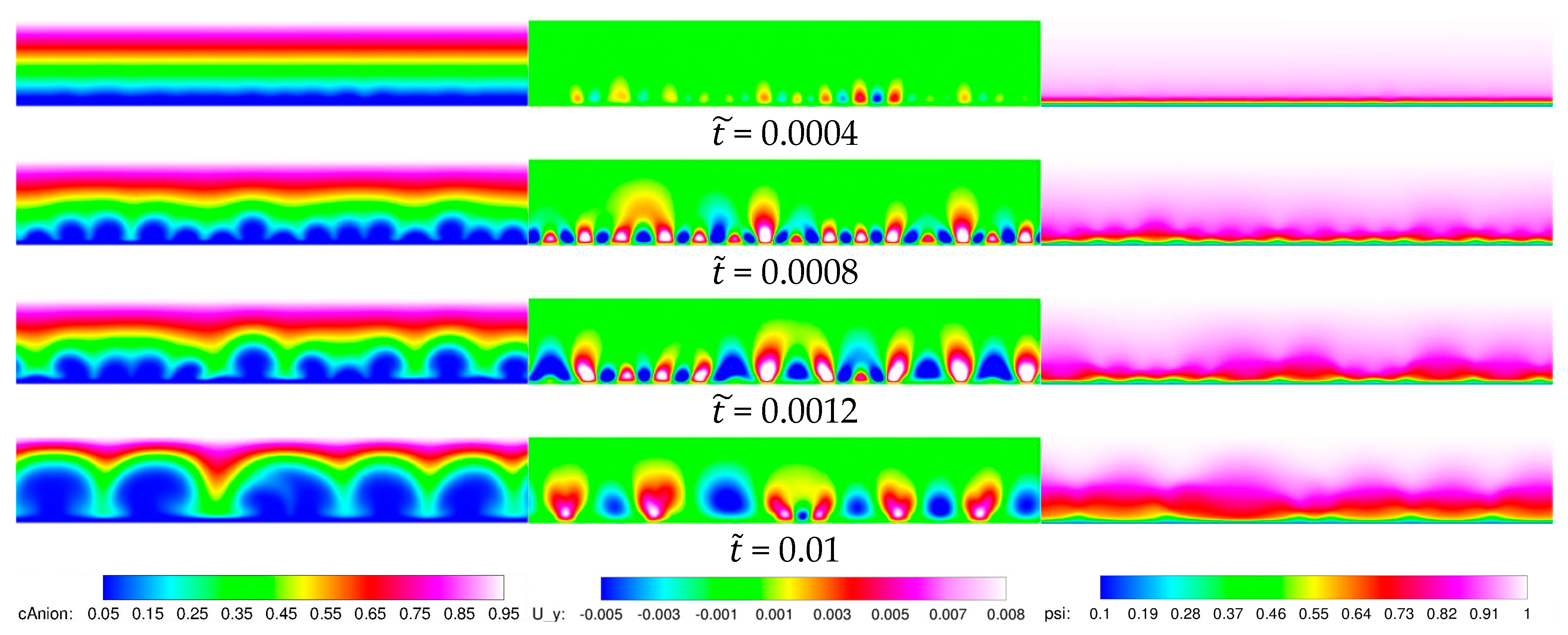
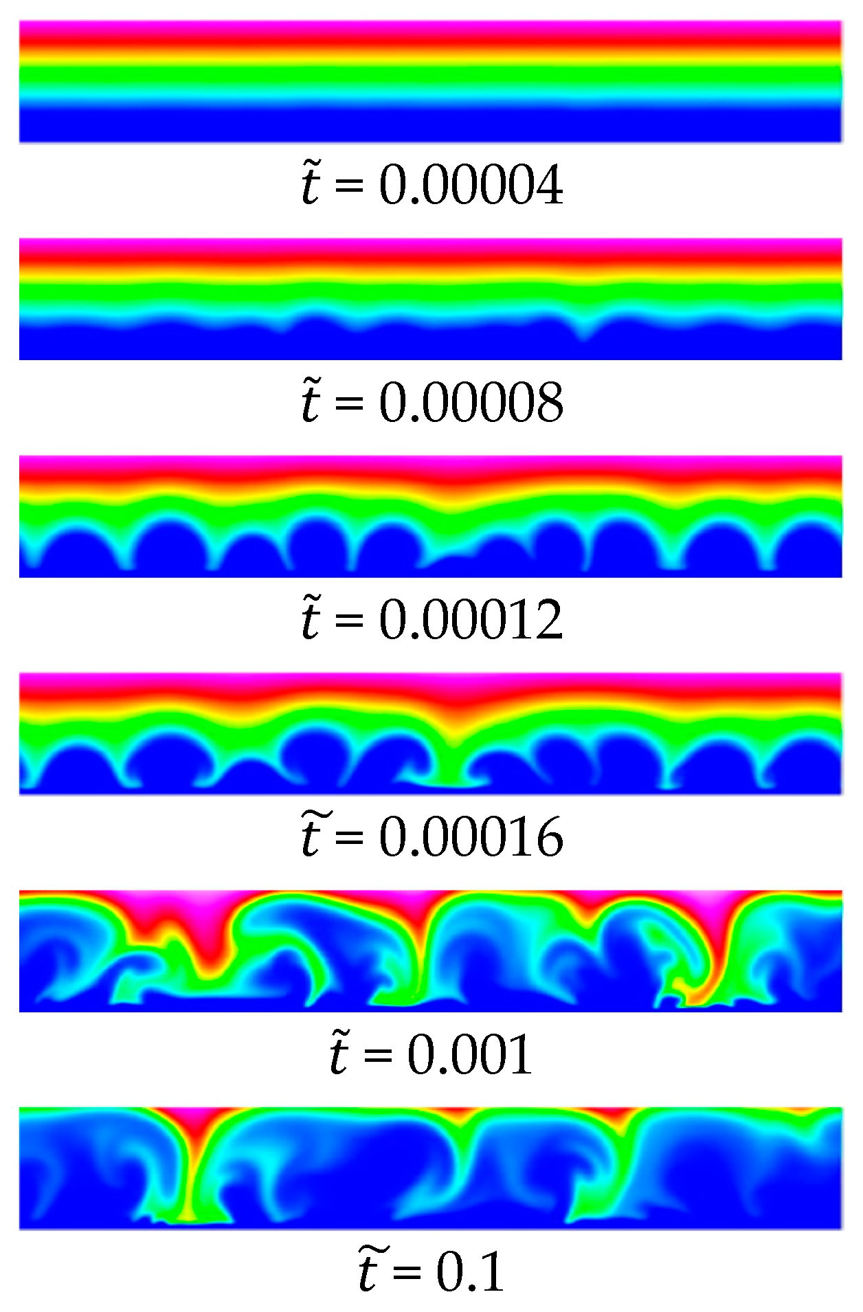
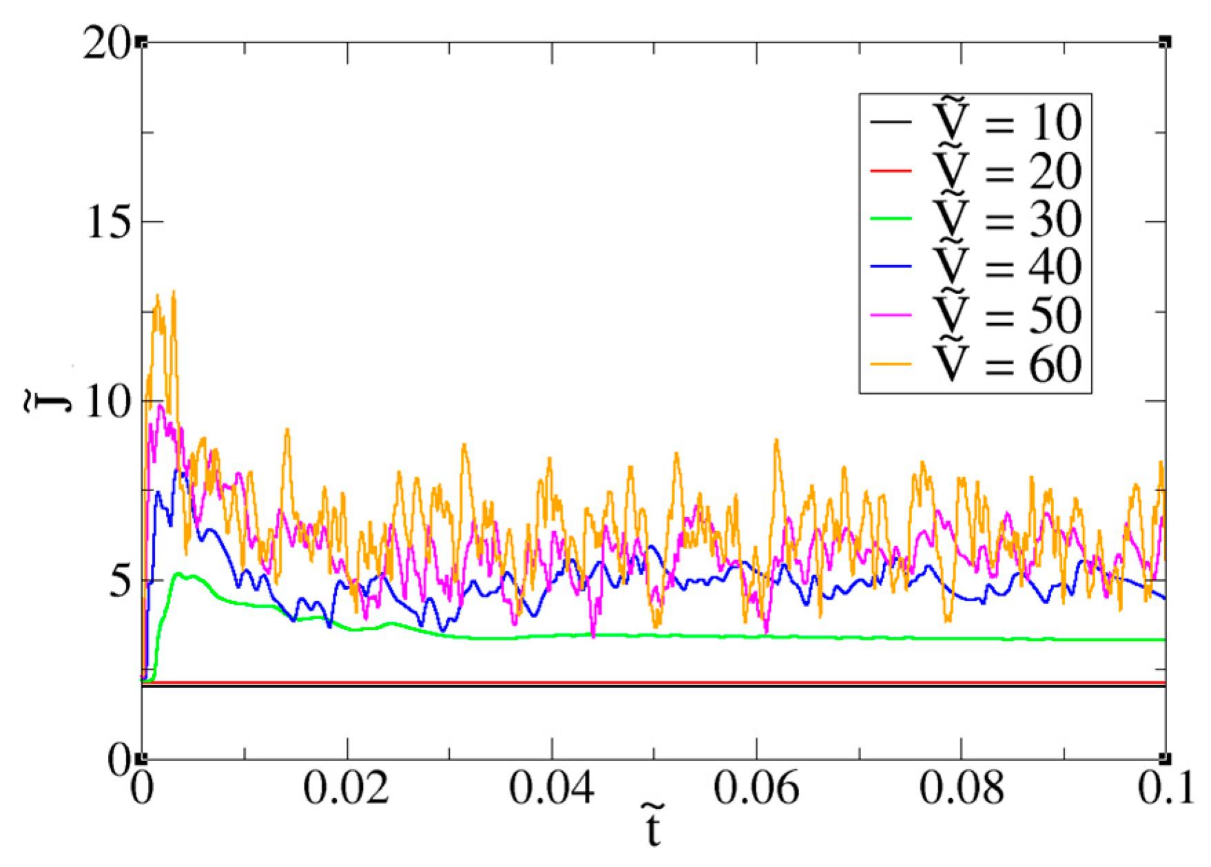
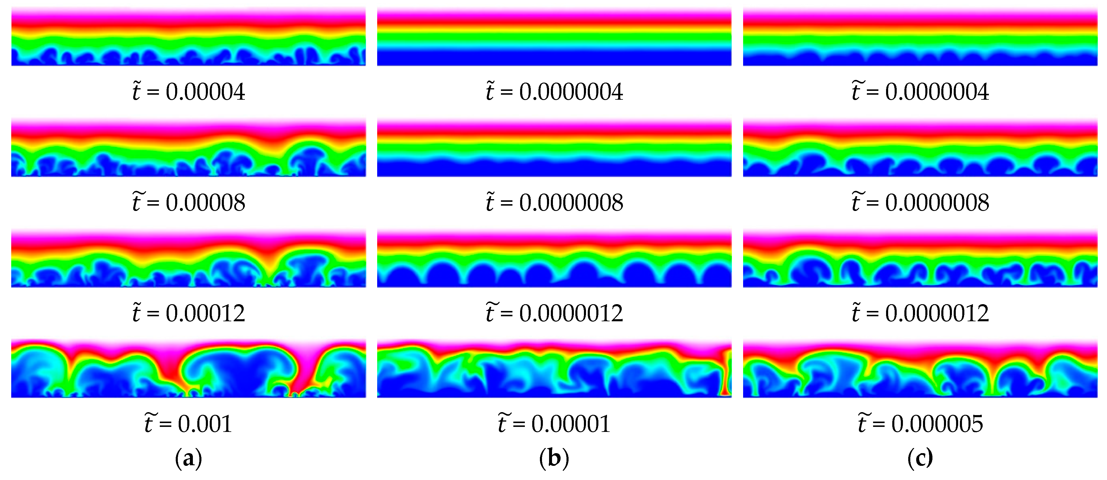
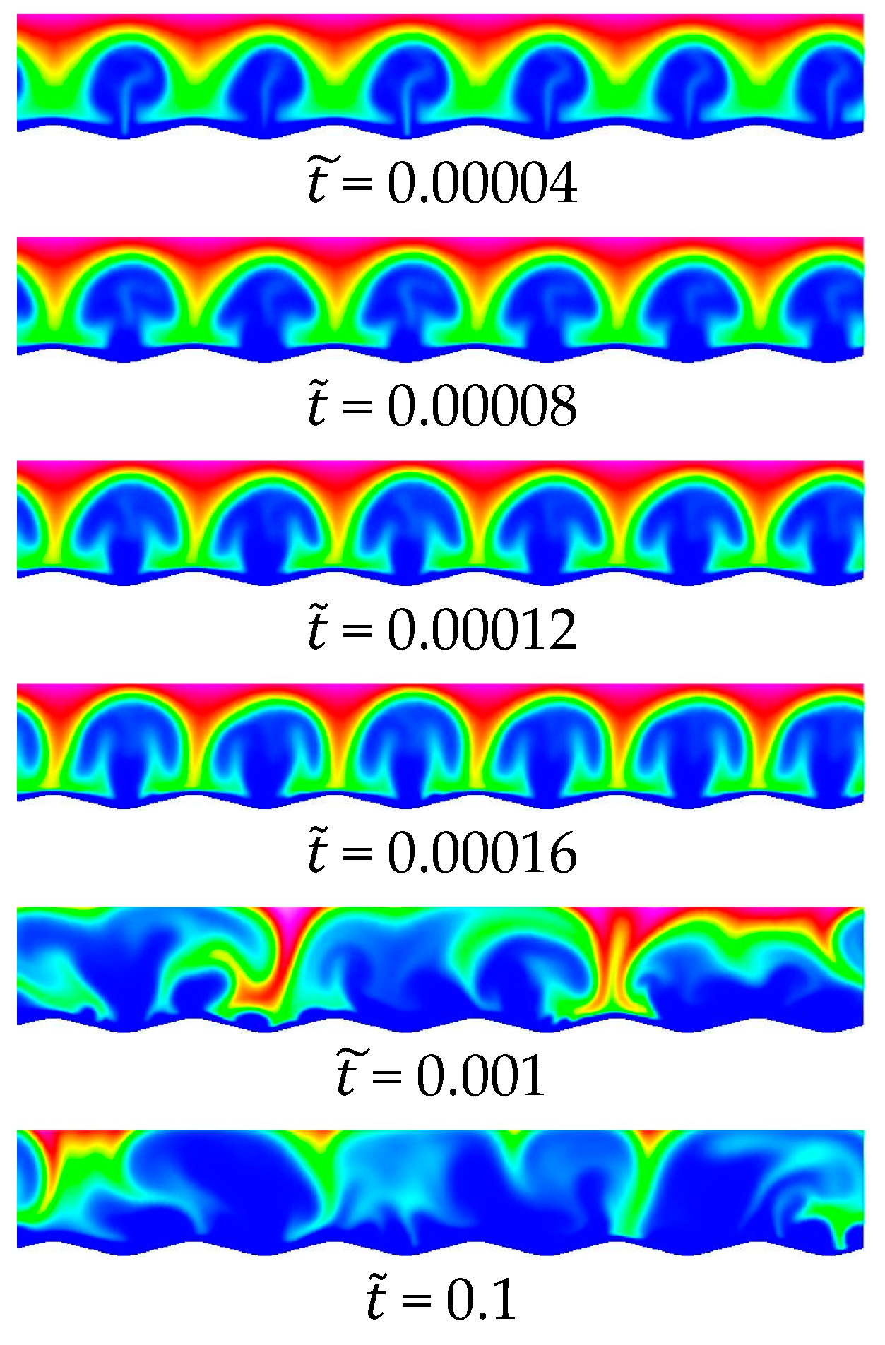
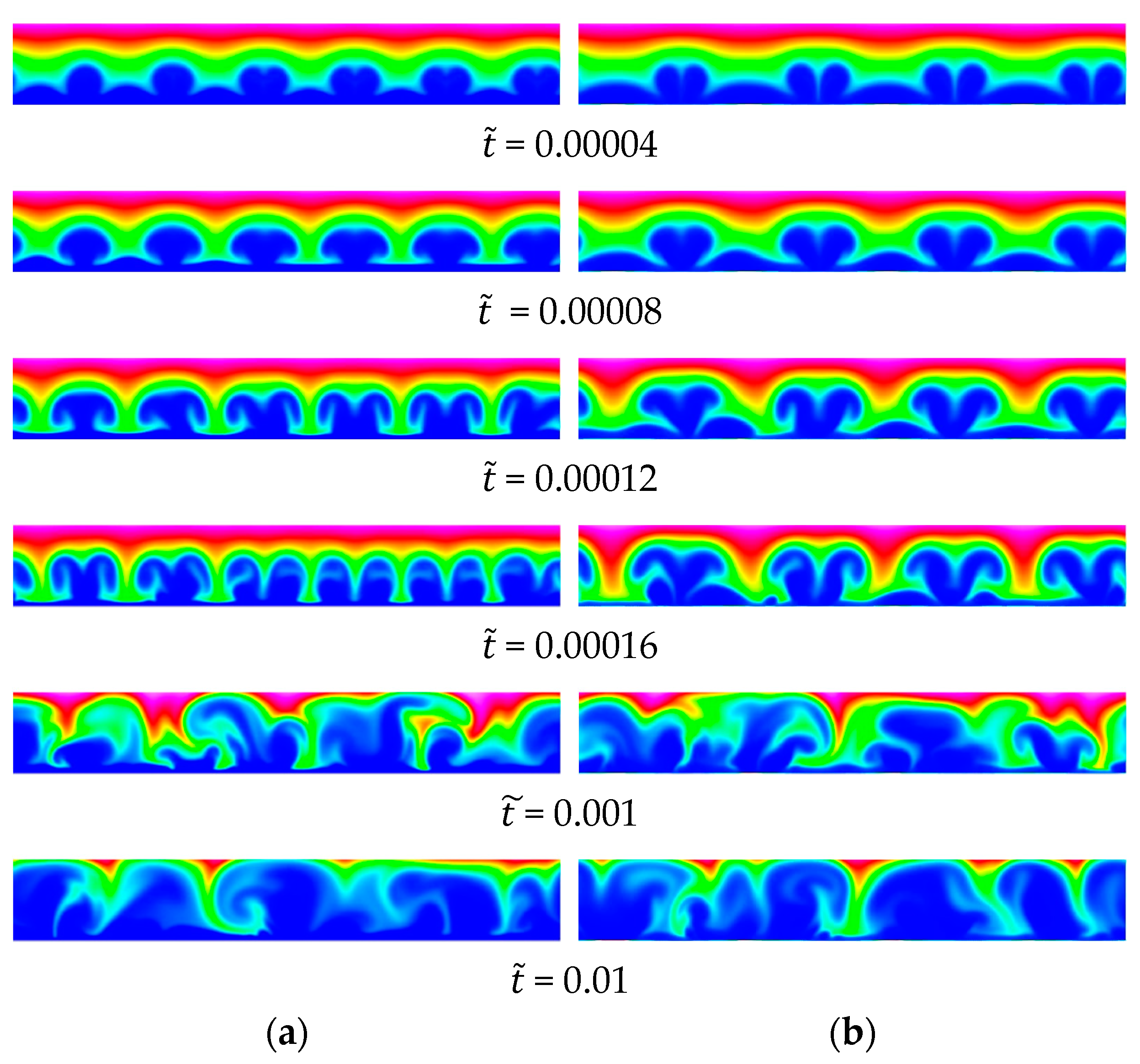
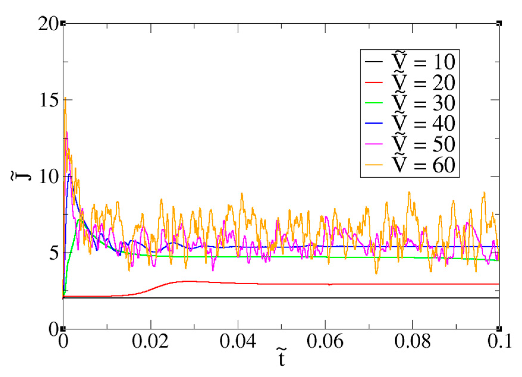
The overlimiting regime in electrodialysis (ED) is associated with the appearance of electroconvective structures near the membranes. The structures are caused by an electrokinetic instability (EKI). The present two-dimensional (2-D) simulations of a generic two-species problem with a smooth ion-selective membrane on the bottom and a water flow channel (reservoir) on the top indicate a dependence of the onset of the EKI on the applied voltage and concentration. With an increasing applied voltage and concentration, the instability becomes stronger and the structures form earlier. The initial perturbations were found to have a well-defined wavelength that is inversely related to the concentration. For very low ion concentrations (), the wavelength was of the order of . For ion concentrations of (moderately brackish water) and (seawater), the wavelength was in the order of .
For ED applications, it is desirable to delay the onset of the overlimiting regime. Similar to hydrodynamic stability problems in fluid mechanics, it was speculated that a favored natural most-amplified wavelength exists. Related research by Saric et al. [
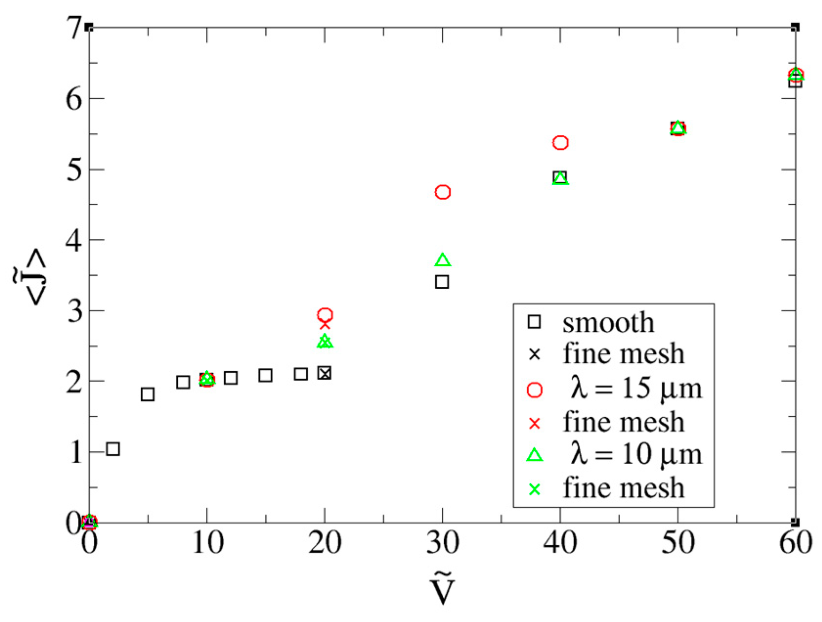
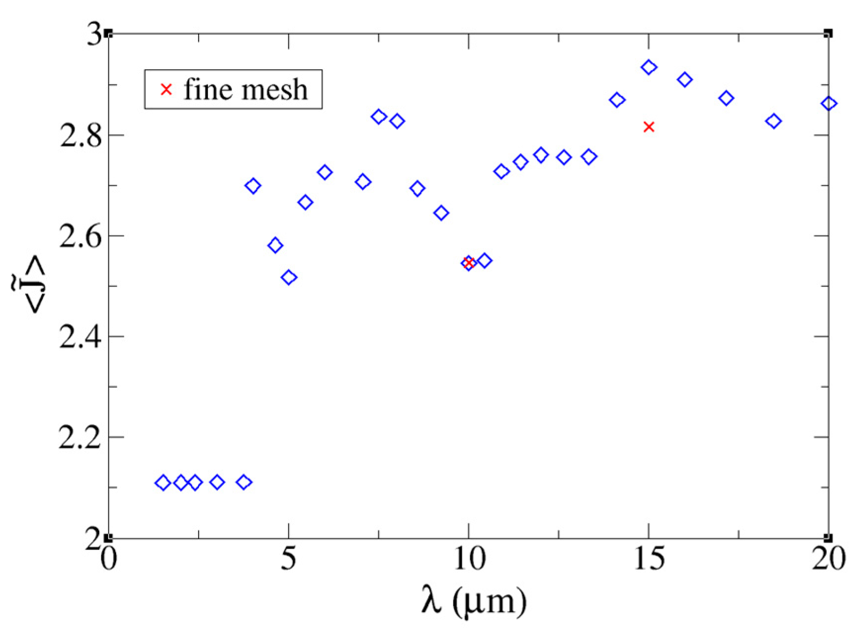
18] of the crossflow instability on swept wings has shown that by forcing a wavelength that is incommensurate with the wavelength of the most amplified natural disturbances, the appearance of nonlinear flow structures can be delayed. Whether the same idea can be transferred to ED applications was investigated. In the present simulations, disturbances were introduced through a 2-D periodic waviness of the membrane surface. It was found that a very minute waviness amplitude had a large effect on the initial growth of the disturbances and the time- and area-averaged current density. When the wavelength was
,
, or
, in agreement with Rubinstein and Zaltzman [
8], the current density increased and the overlimiting regime set in at a lower voltage. It was speculated that for these cases, the initial amplitude of the naturally occurring unstable mode was increased. Forcing with a wavelength of
and
, on the other hand, delayed the formation of the structures and the onset of the overlimiting regime. When the wavelength of the membrane waviness was below approximately
, it had no effect on the current density and the smooth membrane result was recovered.
Membranes are never perfectly smooth. The proposed simulations show a clear dependence of the minimum voltage for the onset of the EKI and thus the overlimiting regime on the geometric surface properties of the membrane. The membrane fine structure (order of
for low concentrations and
for higher concentrations) has implications for the onset of the overlimiting regime and the current density. It was found that by adding fine-scale structures to the membrane surface, the onset of the instability can be controlled. Compared to Güler et al. [
21], the wavelength is several orders of magnitude smaller and the control is based on a different physical mechanism. Whether such membrane surface modifications are feasible remains to be seen. Finally, the 2-D assumption was made for the present parameter study. The extension to 3-D will be explored in the future.


