Site Selection of Aquifer Thermal Energy Storage Systems in Shallow Groundwater Conditions


1
Department of Civil, Environmental and Natural Resources Engineering, Lulea University of Technology, 97187 Luleå, Sweden
2
College of Engineering/Al-Musaib, University of Babylon, Hillah 51006, Iraq
3
Remote Sensing Center, University of Kufa, Kufa 54003, Iraq
*
Author to whom correspondence should be addressed.
Water 2019, 11(7), 1393; https://doi.org/10.3390/w11071393
Submission received: 18 April 2019
/
Revised: 3 June 2019
/
Accepted: 12 June 2019
/
Published: 6 July 2019
(This article belongs to the Special Issue Water Resources Management Strategy Under Global Change)
Abstract
:Underground thermal energy storage (UTES) systems are well known applications around the world, due to their relation to heating ventilation and air conditioning (HVAC) applications. There are six kinds of UTES systems, they are tank, pit, aquifer, cavern, tubes, and borehole. Apart from the tank, all other kinds are site condition dependent (hydro-geologically and geologically). The aquifer thermal energy storage (ATES) system is a widespread and desirable system, due to its thermal features and feasibility. In spite of all the advantages which it possesses, it has not been adopted in very shallow groundwater (less than 2 m depth) regions, till now, due to the susceptibility of the storage efficiency of these systems to the in-site parameters. This paper aims to find a reliable method that can be used to find the best location to install ATES systems. The concept of the suggested method is based on integrating three methods. They are, the analytical hierarchy process (AHP), the DRASTIC index method, and ArcMap/GIS software. The results from this method include a criterion that summarizes the best location to install an ATES system. This criterion is depicted by ArcMap/GIS software, producing raster maps that specify the best location for the storage system. The suggested method can be used to find the best location to install the thermal storage, especially in susceptible aquifers.
1. Introduction
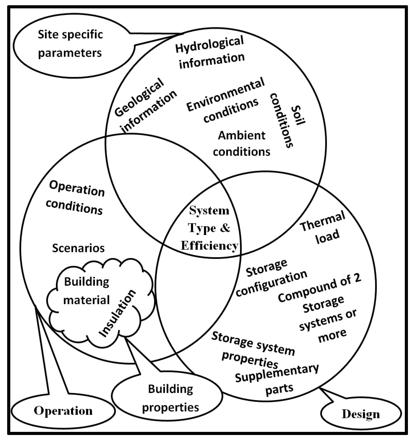
Underground thermal energy storage (UTES) systems are widely used around the world, due to their relations to heating ventilating and air conditioning (HVAC) applications [1]. To achieve the required objectives of these systems, the best design of these systems should be accessed first. The process of determining the best design for any UTES system has two stages, the type selection stage and the site selection stage. In the type selection stage, the best sort of UTES system is determined. There are six kinds of UTES systems, they are: boreholes, aquifer, bit, tank, tubes in clay, and cavern [2,3,4,5]. The selection of a particular type depends on three groups of parameters. They are: Site specific, design, and operation parameters (Figure 1). Apart from site specific parameters, the other two types can be changed through the life time of the system. The site specific parameters, e.g., geological, hydrogeological, and metrological, cannot be changed during the service period of the system. Therefore, the design of the best type should depend, at first consideration, on site specific parameters.
After the type selection stage is finalized, the stage of the best location/site can be initiated. In this stage, the best location to install the system is determined. It depends essentially on the site specific parameters, since the other two groups of parameters (design and operation) can be changed. The site selection should be based on the best efficiency to the system. The best efficiency can be formulated through different approaches. Some of these approaches are energy, cost, return time (payback time), and environment approaches. All these approaches can be summarized in one combined approach, which is the feasible and objective approach. The decision makers can formulate the different approaches, e.g., energy, cost, and environmental, into specific equations, i.e., objective functions, using optimization principles. The different approaches can be represented by many criteria. Considering the environmental approaches, they can be addressed by DRASTIC index [6,7,8]. DRASTIC index refers to the potential vulnerability of the aquifers to be contaminated by the surface contaminants which are leached to the aquifer by the water infiltration from rainfall [6,9,10]. By optimization, the objective function can be solved to find the solution, maximum or minimum value.
As aforementioned, in spite of the importance of site conditions upon the efficiency to the storage system, there is no particular methodology that can be used to specify the best location to install the storage system. Al-Madhlom et al. [11] suggested a method that has not been adopted before.
This paper suggests a new method that can be used to find the best location to install aquifer thermal energy storage (ATES) system. The suggested method has not been adopted till now. The invented method presents the best location as geographic information system (GIS) maps.
The new method requires combining three types of fields of knowledge. They are heat transfer, hydro-geology, and geographic information systems (GIS). In the case that one field is neglected, the method cannot be developed. The installed aquifer thermal energy storage (ATES) systems, till now, did not consider the hydro-geological in-site properties in explicit criterion. The new method summarizes all the effecting parameters in one criterion that can be used to determine the best location to install the thermal storage system.
Underground thermal energy storage (UTES) systems, including aquifer systems, are well known in Europe and in the USA where groundwater is relatively deep. They are used mainly in heating applications (in winter) [12,13,14]. In spite of collected knowledge about these systems, they have not, till now, been used in Middle East. Middle Eastern countries experience high temperatures in summer, which can reach more than 50 °C, and face serious problems in cooling (during summer). This paper suggests a new method that can be used to find the best location to install an aquifer thermal energy storage system. The suggested method can be used efficiently for regions that have shallow groundwater, since the efficiency of the thermal storage in these cases is very affected by the in-site hydro-geological properties.
The objectives of this article are: First, to find the best location to install an aquifer thermal energy storage (ATES) system (main objective). The significance of the suggested method is manifested in shallow groundwater conditions, due to the high susceptibility of storage efficiency of the thermal storage in these conditions. This study considered Babylon province (middle of Iraq), which has shallow groundwater, as a case study area. The second objective is to highlight the effect of depth to groundwater on the results. The third objective is to compare the results of site selection for two regions having different groundwater conditions (shallow and deep). The study considered Karbala province, bordering the Babylon province, as a deep groundwater region.
2. Methodology
As aforementioned, one of the aims of this article is to present a suggested methodology that can be used to find the best location to install an ATES system. The suggested approach is based on two well-known methods, the analytical hierarchy process (AHP) [15], and the DRASTIC index [6]. Furthermore, the process of site selection has four main steps: First, defining objective function with all its weighting factors by using the analytical hierarchy process method; second, checking the validity of all weighting parameters that are found in the first step; third, using DRASTIC index to formulate the in-site conditions; fourth, using ArcMap/GIS to depict the results. The process is described in more details as follows.
2.1. Analytical Hierarchy Process (Weighting Step)
In this stage, the objective equation is specified according to the best efficiency to the storage system. There are different approaches that can be used to define the efficiency to the system. Examples are, storage efficiency, cost, return period, and environmental effect. The objective function can be compounded to represent/satisfy two or more different approaches [16]. The decision makers can list the approaches according to their priorities. Then, they can establish the objective function according to that order of priorities. The different approaches are then assembled and written in terms of controlling parameters (site specific factors). Depending on the resultant equation the best location to install the storage system can be specified. The resultant objective function can be written as follows:
where is the site suitability index factor (dimensionless; its values rate from 0 to 10), is the normalized weight of the in-site factor (dimensionless; its values rate from 0 to 1), and is the rating of the factor (dimensionless; its values rate from 0 to 10).
2.1.1. Defining the Problem
The type of underground thermal energy storage (UTES) system, which is required to be installed, should be defined. In this study, it is the aquifer ATES system. The controlling factors (in-site parameters) that are involved within the objective function are to be deduced. The importance of each in-site factor is decided according to the decision makers’ judgements. Depth to groundwater, seepage velocity, transmissivity, aquifer thickness, type of aquifer, volume of the aquifer, types of groundwater, and temperatures of groundwater are some examples of site specific parameters.
2.1.2. Arranging/Ranking
Site specific parameters should be arranged according to their importance on the site selection. The parameters are ordered from high to low effect. An integer value (rates from 1 to 9) is to be assigned to each parameter (Table 1). Note that, if a parameter has zero influences, it means that the parameter is not comparable with the considered parameters [16]. The high effective parameter is given a larger integer value such as 8 or 9. The parameters that have less influence are assigned to a small integer value like 1 or 2. The parameters which have intermediate influences are assigned to intermediate asset values. In reality, there are many applications that can satisfy this ranking [10]. But, this scale can be changed according to the judgment of the decision makers in the hydro-geo-energy mapping field, i.e., this scale has the flexibility to assign fractional “tad” values in order to refine the scale [9].
2.1.3. Pairwise Matrix
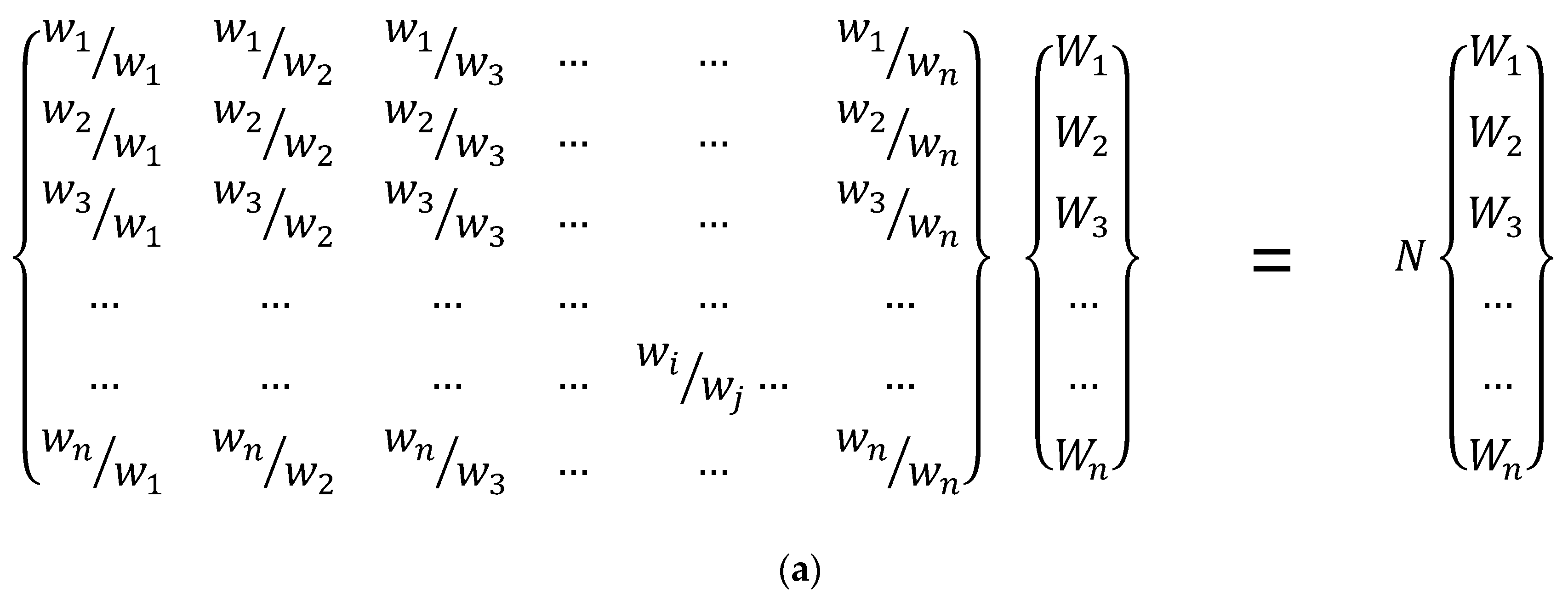
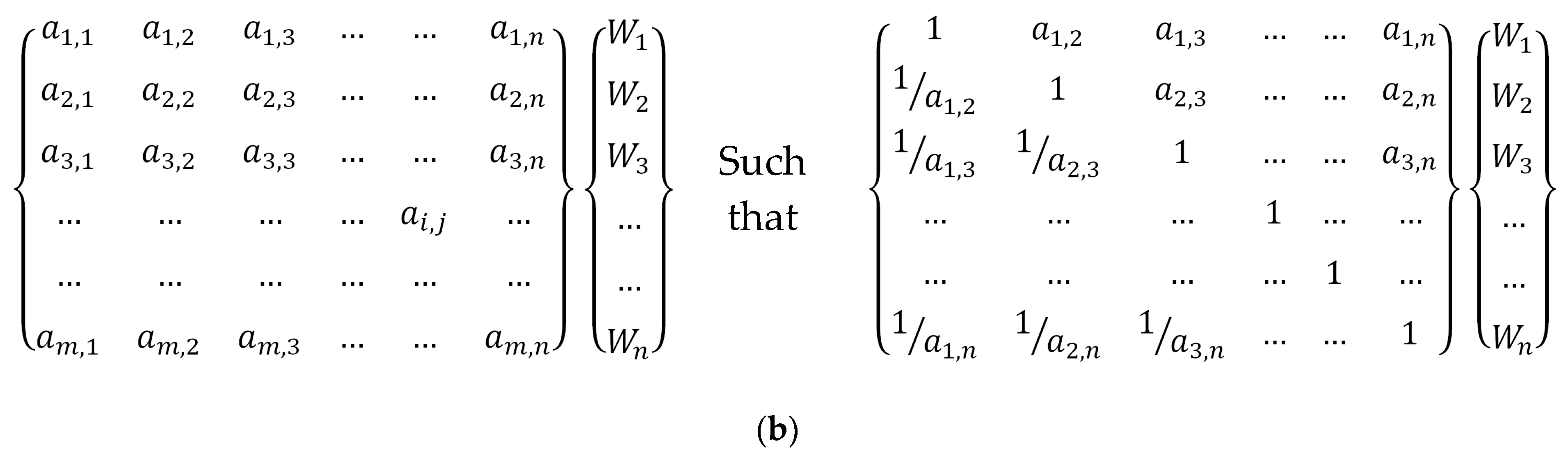
A pairwise comparison matrix should be constructed, which depicts the relationships between the parameters (Figure 2a,b). Priority matrix () (Figure 2a and Equation (2)) can be written in terms of matrix (Figure 2b and Equation (2)) [16].
There is an infinite number of methods, that can be used to derive the vector of priorities from matrix . However, since the emphasis is on the consistency, the eigenvalue formulation (Equation (2)) is to be considered. Consequently, matrix (Figure 2b) can be written in terms of eigenvalue as follows [16]:
and:
where is the priority of the element (Figure 2a), is the matrix of elements () (Figure 2b), is the number of rows or columns in the matrix which equals the number of the considered factors, is the index of the row, is the index of the column (Figure 2b).
2.1.4. Weighting
The weight for each factor is determined by using the pairwise matrix (matrix ) see Figure 2b. The weight of any factor ( is the relative importance or degree of relative importance of that factor compared to the other elements [18]. The weight ( can be found by applying the following equation [19]:
where is the weight of the factor, is the product of row elements, is the number of factors. It equals to the number of the columns or rows within the matrix (Figure 2b).
To normalize the weights produced by Equation (4), Equation (5) is called [15]:
where is the normalized weight of the factor.
2.2. Analytical Hierarchy Process (Check Step)
The consistency of the matrix must be evaluated and verified. To verify the consistency of the matrix, the following steps are applied [15,16].
2.2.1. Lambda (
Lambda (, maximum eigenvalue) is an essential verifying parameter in AHP. It is used for calculating the consistency ratio (CR) of the estimated vector in order to validate the consistency of the pairwise comparison matrix [18]. In other words, it verifies the rational relations between the matrix elements [15,16]. Equation (2) can be written in terms of as follows [16]:
is calculated as follows [18]:
where is the normalized weight of the factor, is the element in the matrix (Figure 2b), is the number of columns in matrix , is the number of rows in matrix . Note that .
2.2.2. Consistency Index (CI)
2.2.3. Consistency Ratio (CR)
The consistency ratio is then calculated by using the following equation [20]:
where is the consistency ratio, is the consistency index, and is the random index.
2.2.4. Comparing the Resultant Consistency Ratio with the Standards
The last step in AHP (check step) is comparing the calculated consistency ratio (CR) with the standards values (maximum values). The maximum values of CR depend upon the orders of the matrix, it is 0.05 for the 3rd order, 0.08 for 4th order, and 0.1 for 5th order and more [18]. The consistency ratio should be less than the maximum values otherwise the matrix will be inconsistent.
When the matrix has an acceptable consistency, it implies that the adjustments in the matrix elements are small compared to the actual values of the eigenvector entries [15,16]. Whilst the inconsistent matrix means that there is inconsistency in the relations between the elements of the matrix. In other words, the hydrogeological and geological parameters have an inconsistent relation between them. Consequently, an inconsistent matrix does not satisfy Equation (10):
where is the importance of the alternative over alternative , is the importance of the alternative over alternative , is the importance of the alternative over alternative [15,16].
In case the matrix is inconsistent, then the process is initiated from ranking step (2.1.2) by changing the ranking (priority of the parameters) to produce a matrix that satisfies Equations (9) and (10). Otherwise, if the matrix is consistent, the process is turned to the next step (DRASTIC step).
2.3. DRASTIC Step
By approving the consistency of the pairwise matrix, the DRASTIC step can be initiated. This phase consists of the following.
2.3.1. Ranging
In ranging, each governing factor is classified (categorized) either quantitatively into numerical ranges, or qualitatively into significant classes according to its impact on site selection [6]. This step is based on the decision makers’ judgement. The results from this step are either a qualitative or quantitative assessment. Here, the factors are groundwater and bedrock depth, transmissivity, groundwater salinity, and thermal and hydraulic conductivity of the deposits, and are of type quantity. Soil and groundwater type, aquifer media and type and the vadose zone media are quality based site specific factors. Each of site specific factors (qualitative and quantitative) can be divided into identified ranges.
2.3.2. Rating
After completing ranging, the rating of each range is processed. Rating means assigning a rank/weight that can be an integer value, for each controlling parameter range. Rating depends on the relative significance of each range in the site selection. The rating includes both ranges, quantitative and qualitative. The rating is executed by assigning an index for each range. The assigned index range from 1 to 10 is based on the relative importance of that range. High index (e.g., 10) means significant importance, whilst the low index (e.g., 1) means low importance. It is possible to unite/normalize rating by dividing rating parameters by 10 (the maximum scale for rating). The site suitability index in this case ranges from 0 to 1.
The scale 1 to 10 can be changed according to the decision makers’ judgement, the importance of the factor, and the range of the factor that should be covered (length). As an example, scaling 1 to 100 can be used. Another way to change the scale is by using “tad” rating. “Tad” rating refers to when the fractions are evoked in the rating process, i.e., using fractional numbers like 1.7, 6.8, 9.6, 4.2.
If one range is assigned to a zero value rating, then the hydro-geological parameter within that range has no effect upon the site selection.
The different factors can have different rating scale depending on the importance of that factor and the decision makers’ judgement. But, in this case all these scales should be normalized to general/unified scale range.
The method explained in this paper is based on 1 to 10 scale, not on the 0 to 1 scale. By executing rating, Equation (1) becomes ready to be performed by ArcMap/GIS.
2.4. ArcMap/GIS Step
ArcMap is the main application from the three applications that ArcGIS has. The other two applications are ArcGlobe and ArcScene. ArcMap is used for mapping, editing, analysis, and data management by utilizing its 19 toolboxes [22]. The spatial analyst tool box is a significant box from ArcMap toolboxes.
The spatial analyst box is the heart and the soul of ArcGIS. It provides a rich set of spatial analysis and modeling tools (170 tools in 23 toolsets). These tools can be used to perform different methods/equations on the map of both raster (cell-based) and feature (vector) data types [23,24,25]. The spatial analyst tools box is the main box that is used in this step.
There is an additional perspective that should be considered in the process of thermal storage site selection. It is the potential conflict between the available infrastructures in the region and the considered thermal storage. In other words, there are some sites that should be avoided/excluded from the areas/locations list of thermal storage site selection. The excluded locations are those of infrastructures and natural resources, e.g., oil pipes, electricity mainlines, highway roads, rivers, rainfall drainage networks, sewage drainage systems, and landfills. To introduce the effect of these infrastructures, the buffer tool within ArcMap/GIS can be used. This tool can exclude specified regions from the resultant site selection [26]. Since the aim of this paper is to explain a methodology that can be used for thermal storage site selection and to simplify the site selection process, this perspective was not considered in this paper.
The ArcMap/GIS step includes the following.
2.4.1. Preparing the Data
To initiate this step, essential information (such as well logs and maps) regarding the considered parameters should be available. These information are the results from preliminary survey or previous works/studies. The information can be ready maps or excel files. In the latter case (excel files), the data is produced from a group of wells that are available within the study area. The data include site coordinates (geographical or projected system) and the values of the considered in-site parameters. The excel files are then imported by ArcMap/GIS software.
2.4.2. Projecting the Wells
After importing the excel files to ArcMap/GIS software, the wells are projected on a desired coordinate system. The one used in this study is the universal transverse Mercator (UTM), specifically, world position system WSG1984 UTM zone 38N [27].
2.4.3. Interpolation and Ranging
Then, the maps which depict the layers of different in-site parameters are produced by using the interpolation tool (kriging tool) within the spatial analysis tools. Each layer/map of a single hydro-geological parameter is classified into different ranges according to the ranging specified in step (2.3.1).
2.4.4. Reclassifying
This step defines the effect of each range, within each hydro-geological parameter, on the site selection process. Hereby each range is assigned to a single quantitative value according to rating classes in rating step (2.3.2). To perform this step, the reclassify tool within reclass set/spatial analysis tools is used. The results from this step are maps, which are similar to interpolation and ranging (step 2.4.3) but with rates instead of ranges, i.e., different legends.
2.4.5. Map Algebra
Finally, the raster calculator tool within the map algebra set/spatial analysis tools is used to produce the site selection map. Using this tool, Equation (1) can be applied easily. Since, within Equation (1) represents the normalized weight factor , which is produced in step (2.1.4), in the same equation represents the rated layers within step (2.4.4). This tool requires that all the input maps (layers) are as raster maps. The resultant map, which represents the site selection map, contains pixels that possess a 1 to 10 ranking. The most suitable site has the highest rank.
3. Case Study
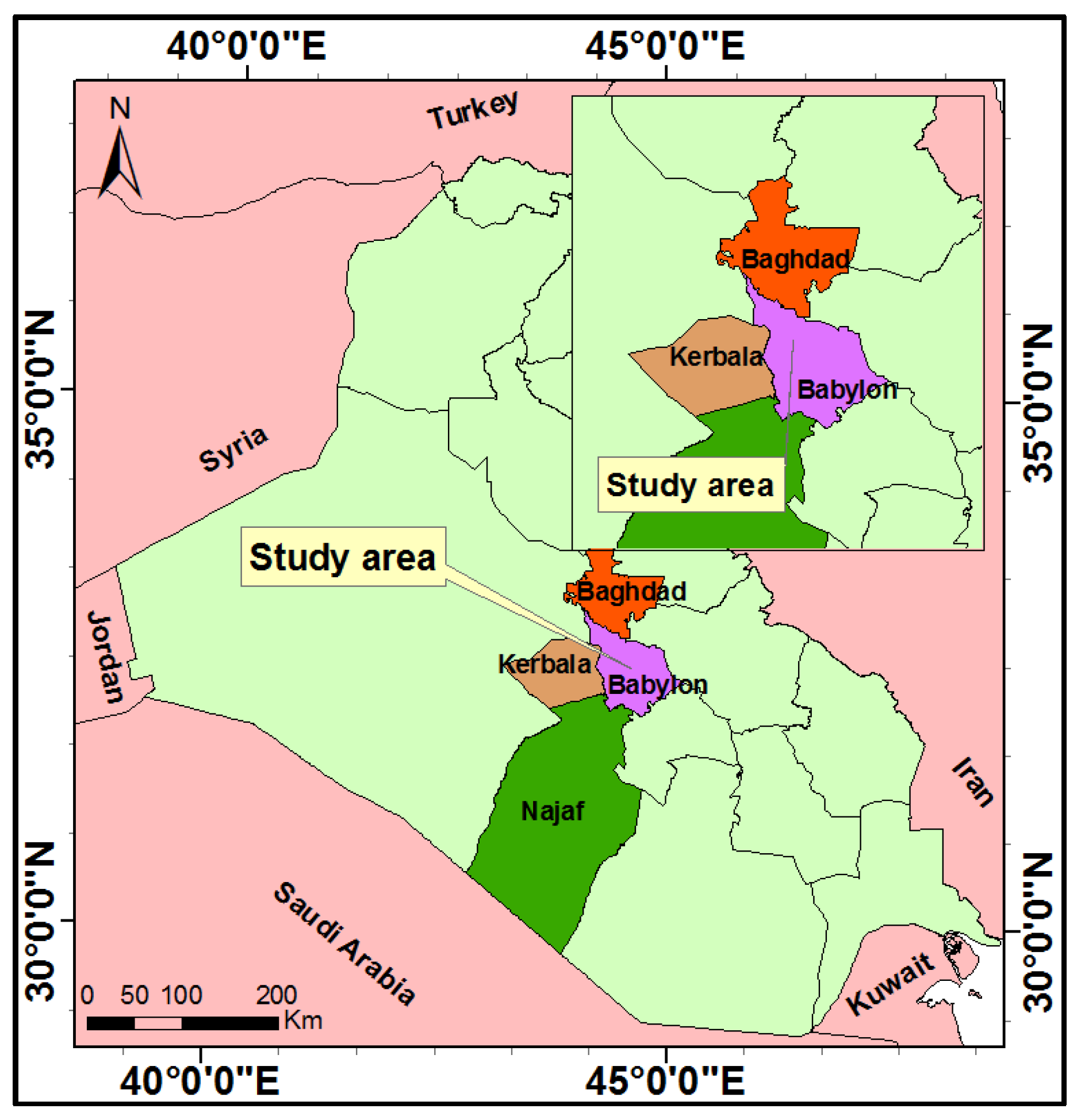
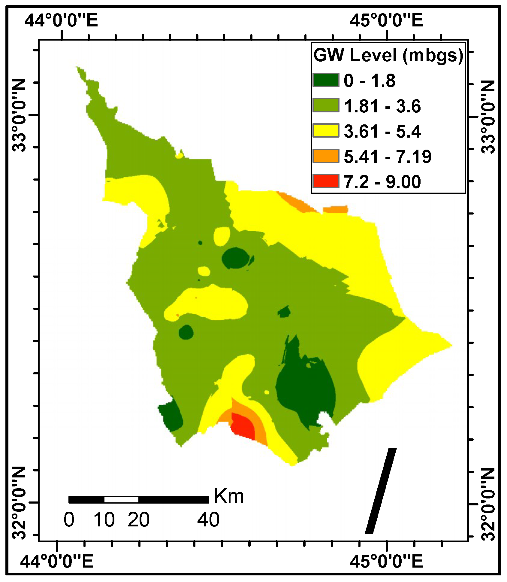
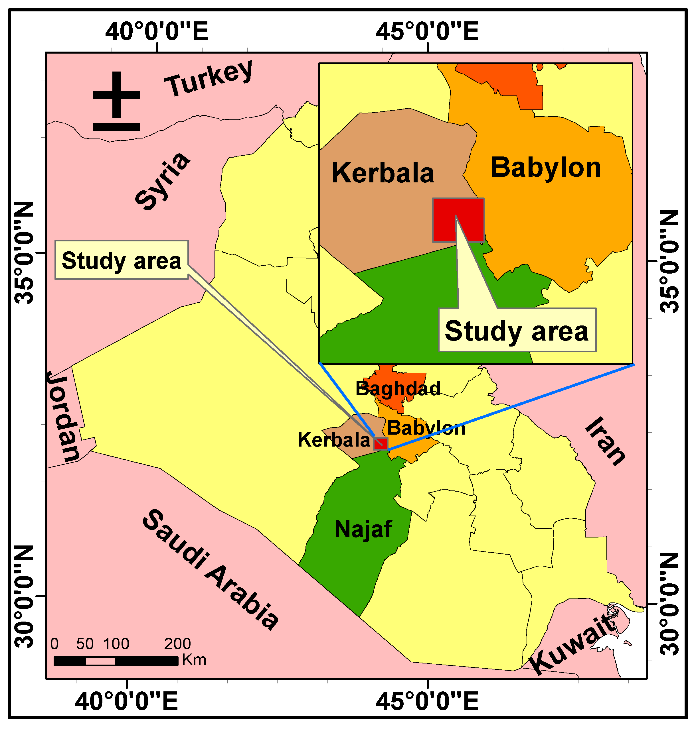
To achieve the aims behind this paper, specifically by demonstrating the suggested method for site selection of an aquifer thermal storage in shallow groundwater region, Babylon province (in the middle of Iraq, Figure 3) was selected as the study area. Babylon province is one of the famous cities in the history of civilization. Babylon province is found near the ruins of the old city. Babylon province has an area of 5134 km2, and a population of about 2 million [28]. The groundwater level is very shallow in Babylon province. It is less than 2 meters in some locations as shown in Figure 4.
This province, as in other provinces of Iraq, has a serious problem in the electricity sector. The energy generated is much lower than the demand [29]. Over the past decades, there have been different reasons behind this problem. But after 2003 (Second Golf War), the significant reason behind this problem is the huge overloading due to heating ventilating and air conditioning (HVAC) applications in summer and winter [30].
It is believed that the problem of electricity deficiency in Iraq can be substantially solved by using underground thermal energy storage (UTES) techniques [28].
Now two questions are highlighted:
- Where is the best location to install an ATES system in Babylon province?
- How can the best location be chosen?
Babylon province was considered as a study area to apply the suggested method. The application was carried out as follows:
3.1. Identifying the Problem
The problem can be formulated in the question: Where is the best location to install an aquifer thermal energy storage system in Babylon province? To answer this question, the parameters that affect the site selection must be listed first. There are many parameters that can affect the site selection process. These parameters can be arranged in three groups. They are design, operation, and hydro-geological in-site parameters (Figure 1). Apart from hydro-geological parameters, the other two groups are totally/partly changeable during the life time of the system. This means that the hydro-geological in-site parameters cannot be changed during the life period of the storage system. Therefore, they are very important to consider within the site selection process. Some examples of in-site parameters that are involved within the site selection process are depth to groundwater, seepage velocity, transmissivity, aquifer thickness, type of aquifer, volume of the aquifer, types of groundwater, and temperature of groundwater. To simplify the process, just four in-site parameters were considered. They were depth to groundwater, transmissivity, seepage velocity, and aquifer saturated thickness.
3.2. Arranging/Ranking
In order to assign an accurate priority to each site specific parameter, the influences of each parameter on the storage system efficiency should be well considered and analyzed.
The depth to groundwater affects the surface thermal losses. Surface thermal losses are the losses that generated a leak from the thermal stored energy to the ground surface. The leak is produced due to the thermal gradient between the thermal storage and the ground surface. When the distance between the storage and the ground surface is small, the thermal gradient is high and the losses are large [31]. The depth of groundwater also effects the digging cost, and the relation between these two variables is proportional. The depth to the groundwater also effects the thermal storage capacity, through affecting the hydraulic conductivity. Since the hydraulic conductivity, in general, decreases with depth of the soil. Hydraulic conductivity effects the peak thermal loads that can be covered by the storage system. Peak load is proportionally affected by hydraulic conductivity.
The groundwater depth fluctuates according to the thermal loads of the system. As an example, the large thermal loads require large storage volume and high pumping rate, which produce high fluctuations in groundwater depths. In addition, the fluctuation in groundwater depths depend on the in-site hydro-geological properties like hydraulic conductivity and porosity [32].
Seepage velocity affects the advection losses. Advection is the rate of bulk groundwater flow. The thermal advection losses are the losses that are produced by advection [33]. Spread rate of the leached contaminants is proportional to seepage velocity [34].
Transmissivity affects the peak loads that can be covered by the system. High transmissivity leads to high loads that can be covered.
Aquifer saturated thickness effects control the water extraction rate, which effects the shape of the storage, the served thermal loads, and the peak loads.
The influences of the four considered site specific parameters can be summarized in Table 3.
The influences of the four considered site specific parameters are explained in Table 3. After studying the system of parameters very well, the decision makers can assign a priority for each parameter. It is assumed that, according to their opinion, the controlling parameters are arranged according to the priority as in Table 3.
3.3. Pairwise Matrix
3.4. Weighting
3.5. Lambda (
To check the consistency of the pairwise matrix, i.e., there are consistent relations between the four hydro-geological site specific parameters, steps 3.5 to 3.8 were used. First, is determined by using Equation (7). The resultant is 4.1901.
3.6. Consistency Index (CI)
Consistency index (CI) can be found by using Equation (8). For this case CI is 0.0634.
3.7. Consistency Ratio (CR)
Consistency ratio (CR) can be found by using Equation (9). To apply Equation (9), random index (RI) should be evaluated first. Table 2 states that for n equals 4, RI is equal to 0.9. Thus, the value of CR is 7.04%.
3.8. Comparing
3.9. Ranging/Classifying
After verifying the consistency of the pairwise matrix, the ranging/classifying step has to be processed. This step is based on the decision makers’ opinions. In this study, it is assumed that each of the four in-site parameters (Table 3) is divided into a specific number of ranges, which are shown in Table 5.
3.10. Rating
After completing the ranging, the process of rating is initiated. By rating each range within the site specific parameters (Table 5, ranges column) it can be assigned to a specific rank depending on its effect on site selection. The rating is managed by the decision makers. For this study, it is assumed that the rating is as in Table 5 (rating column).
3.11. ArcMap/GIS Step
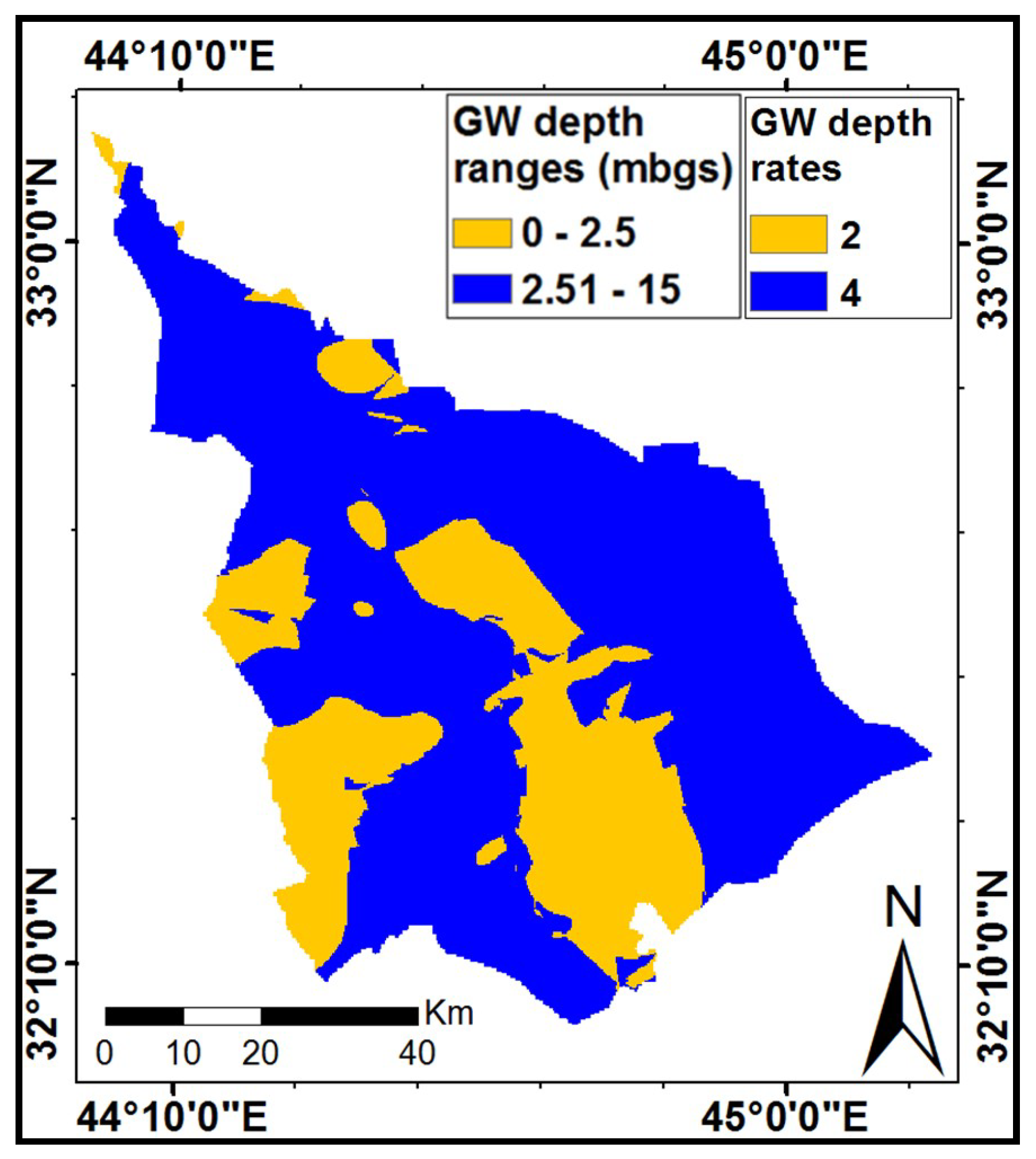
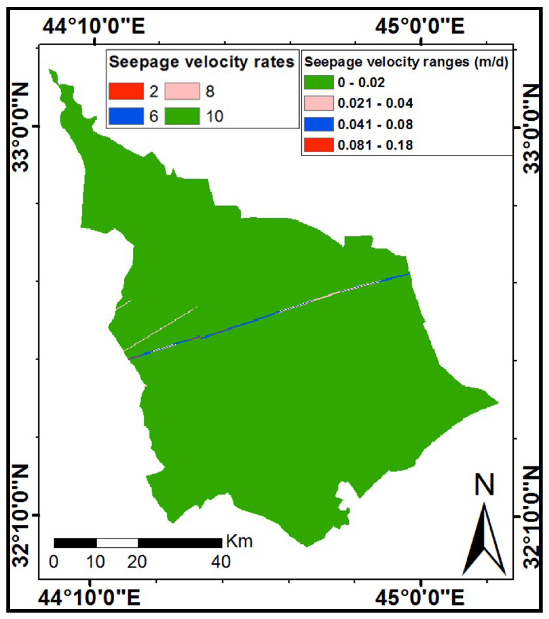
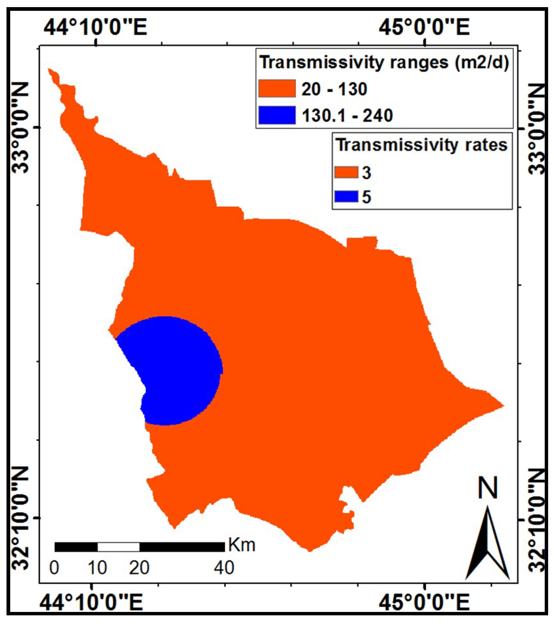
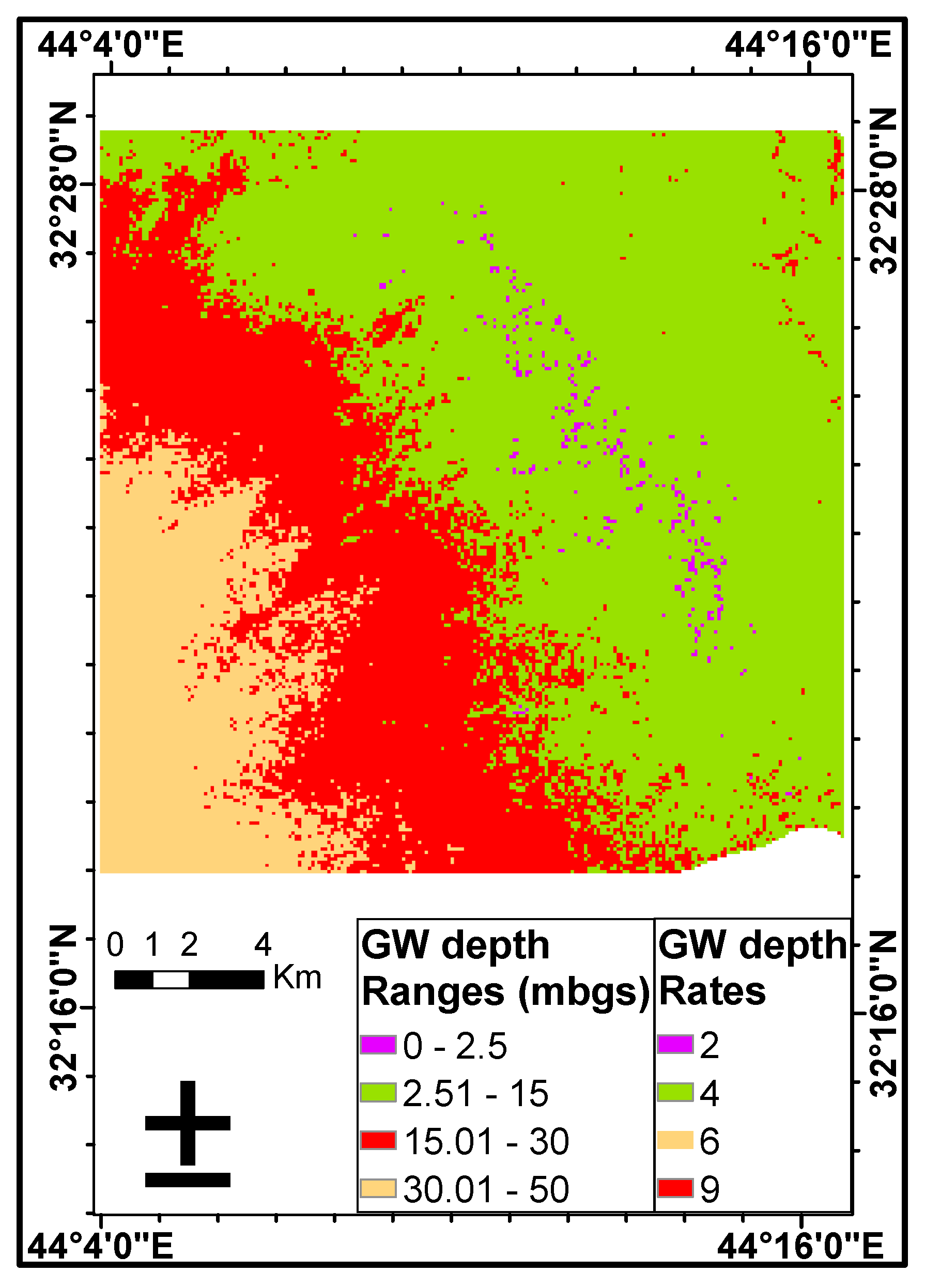
By finalizing the DRASTIC step, the ArcMap/GIS step is initiated. In the ArcMap/GIS step, four layers (maps), groundwater depth, seepage velocity, transmissivity, and saturated thickness were drawn. To draw these maps, specific information was required. This information is, mainly, acquired from the hydrological survey of the region. Wells within and around the region are used to get the required data. The data that was collected from well logs were tabulated within excel tables. Then the excel tables were exported to ArcMap/GIS to be used later, in order to prepare the required four layers. The resultant layers were depicted in the four maps (Figure 5, Figure 6, Figure 7 and Figure 8).
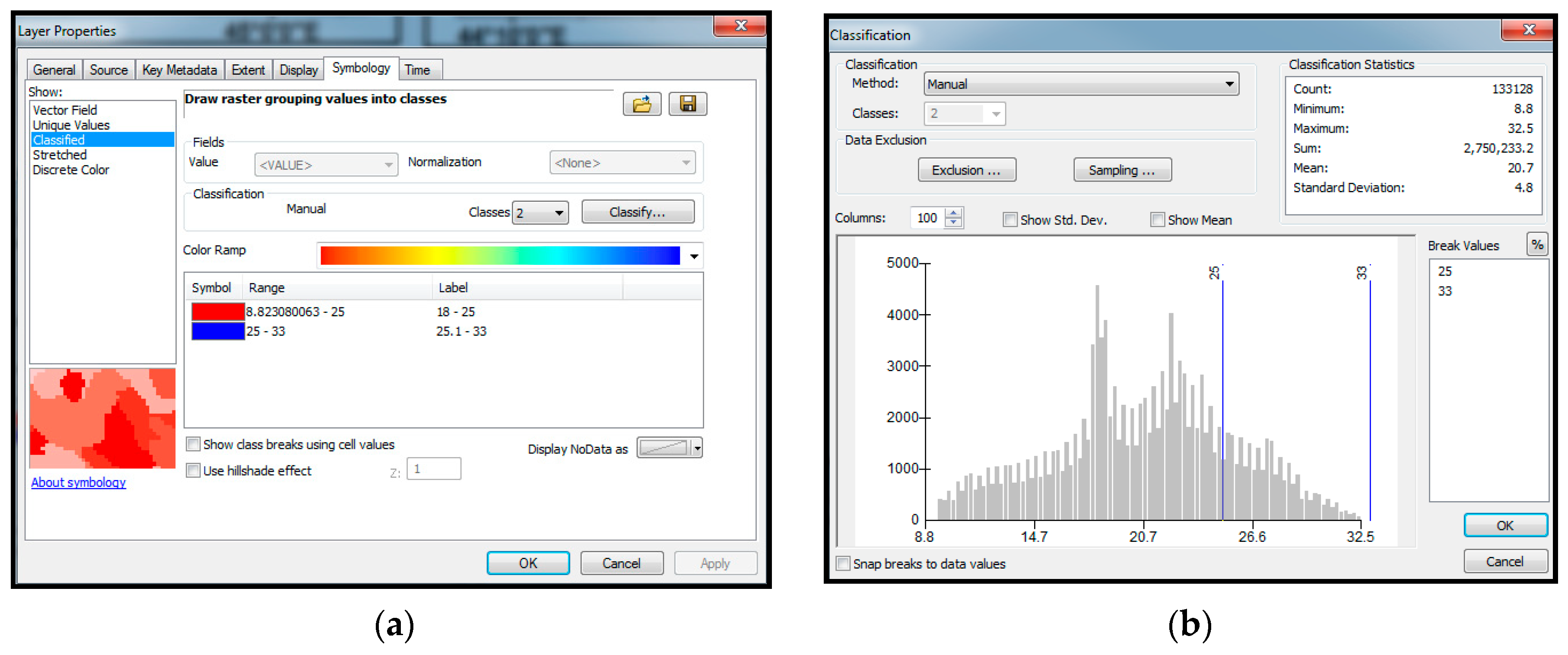
Within the process of preparing the maps of ranges (Figure 5, Figure 6, Figure 7 and Figure 8), classify command (Figure 9) was used to justify the ranges according to Table 5. Classifying command is available within the Layer property window/symbology menu (tab) (Figure 9).
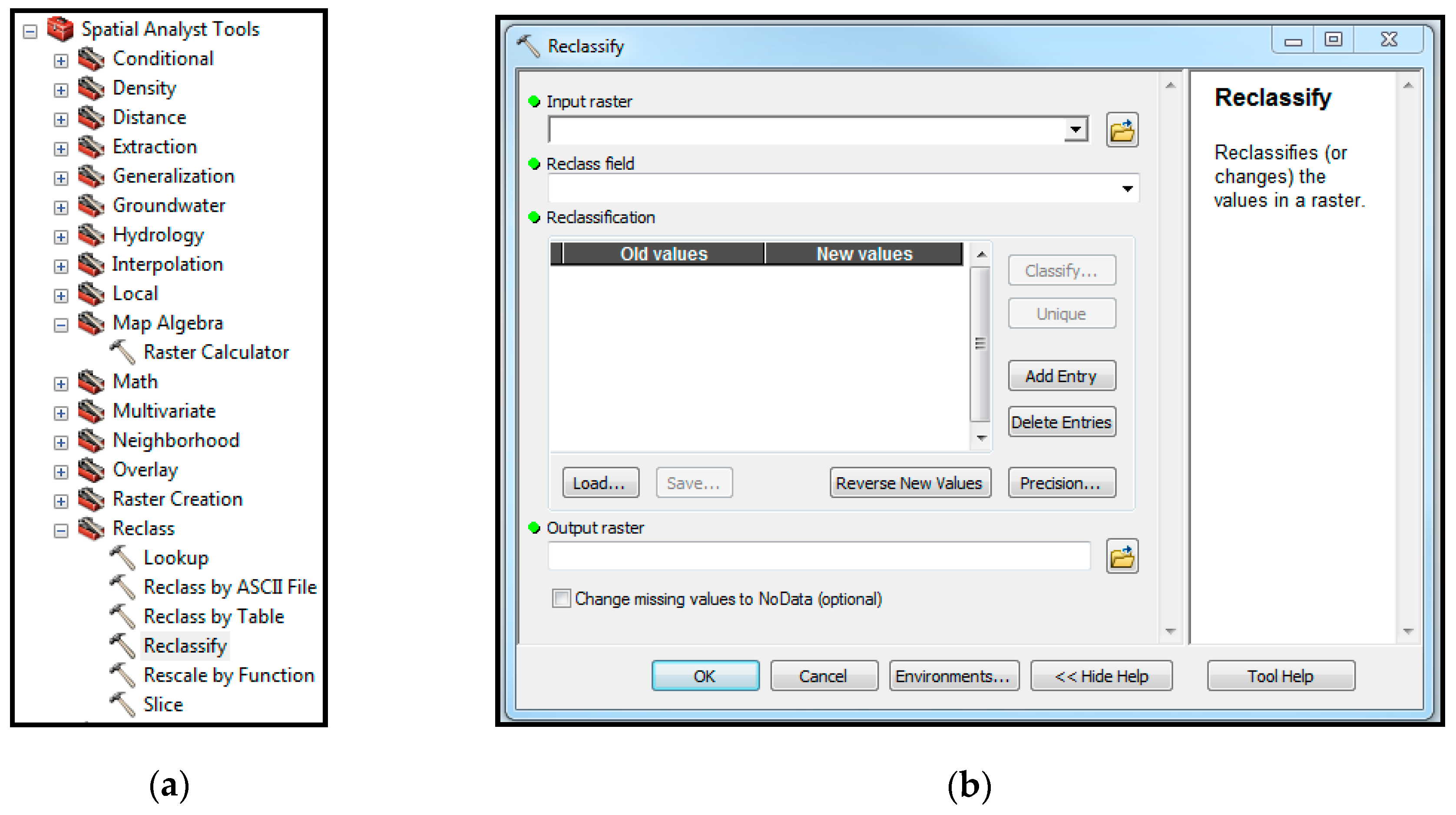
Then, the maps of ranges were used to produce the maps of the rates according to Table 5. A reclassify tool (Figure 10a,b) within the reclass set/spatial analysis tools was used to produce the maps of rates. Again, Figure 5, Figure 6, Figure 7 and Figure 8 were used to depict the resultant maps. But this time, they were used to depict the maps of rates not the maps of ranges by switching the legend of each figure.
4. Results and Discussion
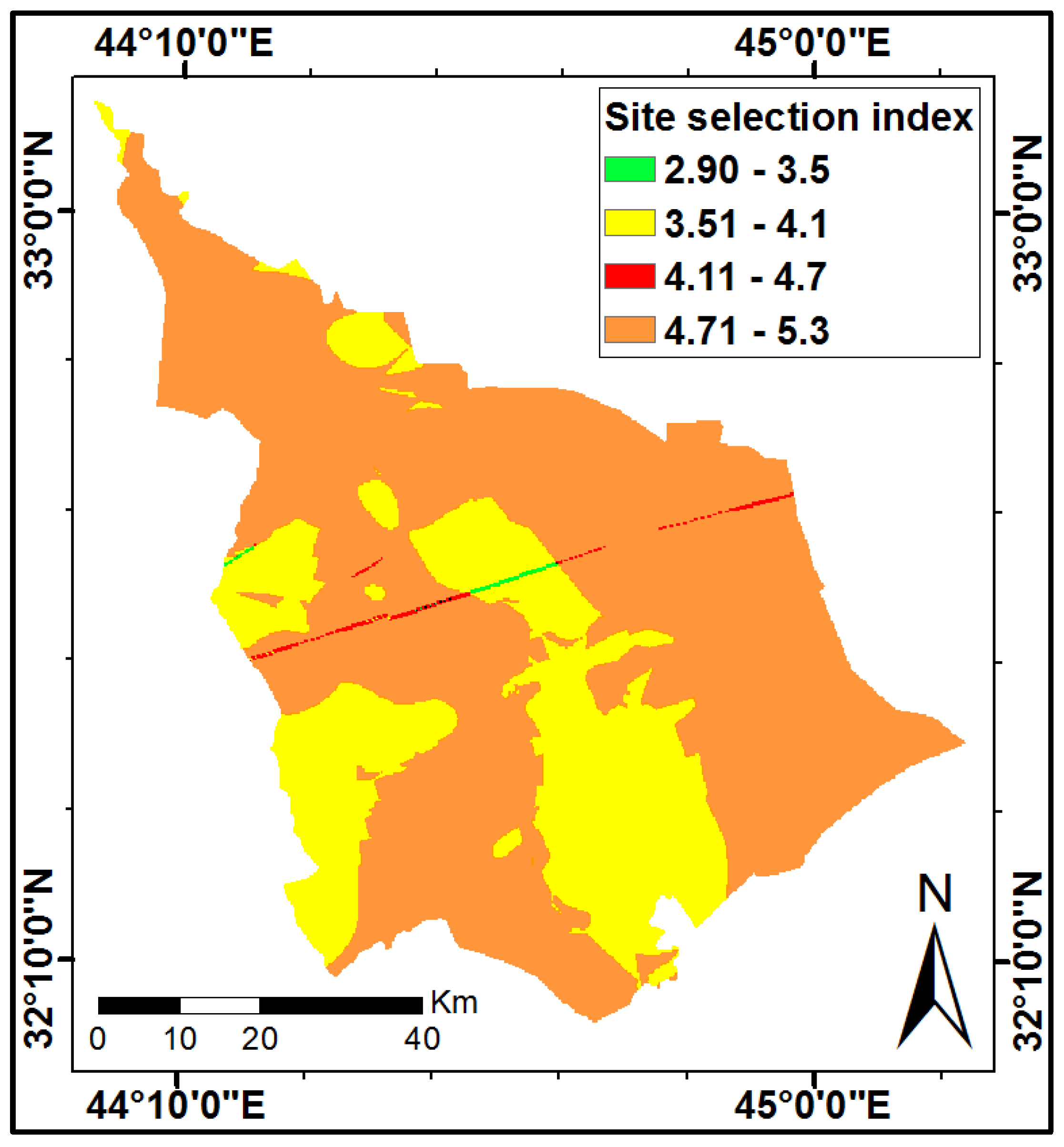
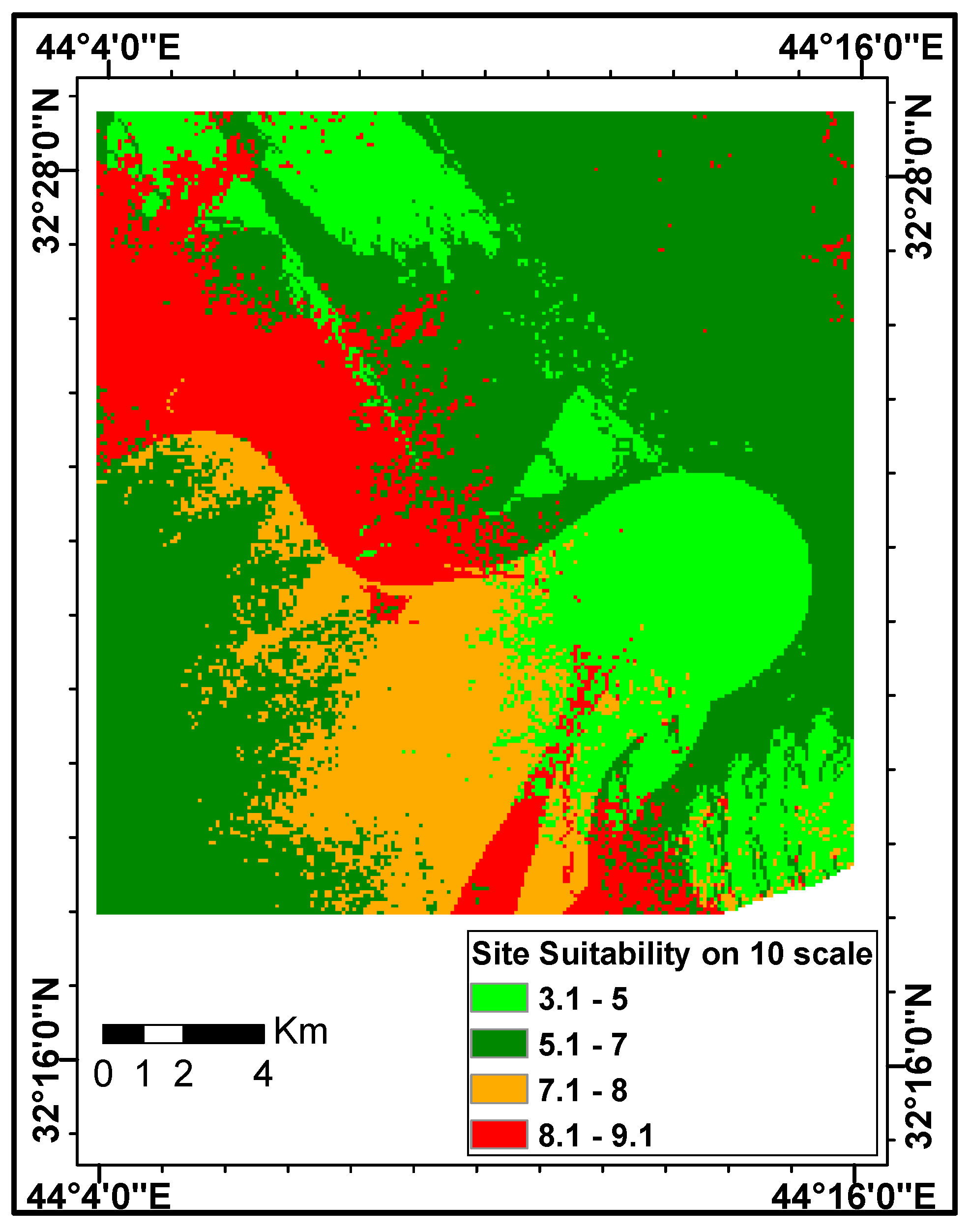
The four rated maps (Figure 5, Figure 6, Figure 7 and Figure 8) were inserted/evoked by the raster calculator tool/map algebra set (Figure 10a) to acquire the map of the ATES system site selection (Figure 11).
The site selection map (Figure 11) demonstrates the best locations to install the thermal storage. The most suitable locations have indexed ranges between 4.71 and 5.3 (Figure 11). To acquire a high accuracy map, the ranges within the legend of map 12 can be increased, and assigned a narrow range for the last range, i.e., 5.11–5.3 instead of 4.71–5.3.
Since the consistency ratio (CR) is 7.04%, which is less than 10%, the matrix (Table 4) has consistent relations between the different geo-hydrological parameters.
The site selection map (Figure 11) has low site selection index values of 5.3 and below on the 1 to 10 scale. The reasons behind this are the high weight of the depth to groundwater 0.654 (Table 4) compared with other factors, and the low rates (2 and 4) of the depth to groundwater map (Figure 4 and Figure 5, Table 5). Transmissivity rates (Figure 7) also negatively affect the site selection map (Figure 11) due to its low rate values. The low transmissivity (transmissivity is equal to “hydraulic conductivity” multiply by “saturated thickness”) is generated from the low hydraulic conductivity since Babylon province has silty clay soil [35,36].
The high weight of the depth to the groundwater (0.654) is generated from assigning high priority rank (9) to that site specific property due to its importance (Table 3). By examining the suggested method, it can be noticed that the depth to groundwater property produces the maximum change in the site selection index. If the two rating values 4 and 9 (Table 5) for this property are considered, then the change in the site selection index is ( (Table 4). The change that is generated from the seepage velocity property, which has the second greatest weight (0.204) (Table 4), is limited to corresponding to the rating values 2 and 6 (Table 5).
To highlight the effect of the depth to groundwater on site selection process, Karbala province neighbouring to Babylon province, was considered (Figure 12). The study area that was considered within Karbala province is depicted as the red square in Figure 12. This region has a deep groundwater table (Figure 13) that reaches to 50 meters below the ground surface (mbgs). Figure 13 demonstrates that the study region within Karbala province has high rates of groundwater depth that reach up to 9 in some locations. These high rates positively affect the resultant map of the thermal storage site selection (Figure 14), producing a high index for site suitability. The site index reached 9 [11], whilst the site suitability index for Babylon province reached 5.3, only as a result of low groundwater depth which ranges from 1.8 to 15 meters below ground surface (mbgs) (Figure 5 and Figure 11).
According to the findings from this study, the suggested method can be used to decrease the electricity demand of the city through installing an aquifer thermal energy storage system. It can be used to find the best location that guarantees the maximum storage efficiency according to the in-site parameters. It can also be used to specify the best locations to install ATES systems in other cities with extremely cold/hot climates, which have huge heating/cooling loads.
5. Conclusions
This work presents a new approach to find the best location to install an aquifer thermal energy storage (ATES) system, particularly in shallow ground water conditions according to site specific parameters. The suggested approach is based on the analytical hierarchy process (AHP), the DRASTIC index method, and ArcMap/GIS software. It assigns a high weighting factor for the depth of the groundwater, due to its significance in determining surface heat losses from the storage and digging cost. In the suggested method, the efficiency can be formulated as an equation. ArcMap/GIS software can be used to apply the formulated equation on the considered area. The final result from this method is a map that depicts the best location to install an aquifer thermal energy storage system. The new approach was applied in shallow (Babylon) and deep ground water conditions. The results showed that the best location, in which ATES system can be installed in, is highly affected by the depth to groundwater property.
Author Contributions
Conceptualization, Q.A.-M.; methodology, Q.A.-M.; software, Q.A.-M.; validation, Q.A.-M., N.A.-A., J.L., and B.N.; formal analysis, Q.A.-M.; investigation, Q.A.-M.; data curation, Q.A.-M.; writing—original draft preparation, Q.A.-M., N.A.-A., J.L., and B.N.; writing—review and editing, Q.A.-M., N.A.-A. and H.M.H.; visualization, Q.A.-M., N.A.-A., J.L., and B.N.; supervision, N.A.-A., J.L. and H.M.H.
Funding
This research is funded by University of Babylon through a scholarship to the first author. Lulea University of Technology supported the use of the facilities at the university to execute this research.
Conflicts of Interest
The authors declare no conflict of interest.
References
- Hesaraki, A.; Holmberg, S.; Haghighat, F. Seasonal thermal energy storage with heat pumps and low temperatures in building projects—A comparative review. Renew. Sustain. Energy Rev. 2015, 43, 1199–1213. [Google Scholar] [CrossRef]
- Rad, F.M.; Fung, A.S. Solar community heating and cooling system with borehole thermal energy storage—Review of systems. Renew. Sustain. Energy Rev. 2016, 60, 1550–1561. [Google Scholar] [CrossRef]
- Nordell, B. Large-scale Thermal Energy Storage. In Proceedings of the WinterCities’2000, Energy and Environment, Luleå, Sweden, 14 February 2000. [Google Scholar]
- Schmidt, T.; Miedaner, O. Solar District Heating Guidelines (Storage-Fact Sheet 7.2); Solar Heating District SHD: Stuttgart, Germany, 2012; pp. 1–13. [Google Scholar]
- Soerensen, P.; Sandrock, M. The role of thermal storage and solar thermal in transition to Co2 neutral hybrid heating and cooling systems in cities. In Proceedings of the 5th Solar District Heating Conference, Graz, Australia, 11–12 April 2018; pp. 1–5. [Google Scholar]
- Aller, L.; Lehr, J.H.; Petty, R.; Bennett, T. DRASTIC: A Standardized System to Evaluate Groundwater Pollution Potential Using Hydro-Geologic Settings; National Water Well Association: Worthington, OH, USA, 1987. [Google Scholar]
- Neshat, A.; Pradhan, B.; Dadras, M. Groundwater vulnerability assessment using an improved DRASTIC method in GIS. Resour. Conserv. Recycl. 2014, 86, 74–86. [Google Scholar] [CrossRef]
- Wu, X.; Li, B.; Ma, C. Assessment of groundwater vulnerability by applying the modified DRASTIC model in Beihai City, China. Environ. Sci. Pollut. Res. 2018, 25, 12713–12727. [Google Scholar] [CrossRef] [PubMed]
- Boufekane, A.; Saighi, O. Application of Groundwater Vulnerability Overlay and Index Methods to the Jijel Plain Area (Algeria). Groundwater 2018, 56, 143–156. [Google Scholar] [CrossRef] [PubMed]
- Barzegar, R.; Moghaddam, A.; Adamowski, J.; Nazemi, A. Delimitation of groundwater zones under contamination risk using a bagged ensemble of optimized DRASTIC frameworks. Environ. Sci. Pollut. Res. 2019, 26, 1–15. [Google Scholar] [CrossRef] [PubMed]
- Al-Madhlom, Q.; Hamza, B.; Al-Ansari, N.; Laue, J.; Nordell, B.; Hussain, H.M. Site Selection Criteria of UTES Systems in Hot Climate. In Proceedings of the European Conference on Soil Mechanics and Geotechnical Engineering (XVII ECSMGE), Reykjavik, Iceland, 1–6 September 2019. (Accepted). [Google Scholar]
- Sarbu, I.; Sebarchievici, C. A comprehensive review of thermal energy storage. Sustainability 2018, 10, 1–32. [Google Scholar]
- Possemiers, M.; Huysmans, M.; Batelaan, O. Influence of Aquifer Thermal Energy Storage on groundwater quality: A review illustrated by seven case studies from Belgium. J. Hydrol. Reg. Stud. 2014, 2, 20–34. [Google Scholar] [CrossRef]
- Gao, L.; Zhao, J.; An, Q.; Liu, X.; Du, Y. Thermal performance of medium-to-high-temperature aquifer thermal energy storage systems. Appl. Therm. Eng. 2019, 146, 898–909. [Google Scholar] [CrossRef]
- Saaty, T.L. Decision Making for Leaders: The Analytic Hierarchy Process for Decisions in a Complex World, 3rd ed.; RWS Publications: Pittsburgh, PA, USA, 2012. [Google Scholar]
- Saaty, T.L.; Vargas, L.G. Models, Methods, Concepts & Applications of the Analytic Hierarchy Process, 2nd ed.; Springer: New York, NY, USA, 2012; pp. 1–40. [Google Scholar]
- Saaty, T.L. Decision making with the analytic hierarchy process. Int. J. Serv. Sci. 2008, 1, 83–98. [Google Scholar] [CrossRef]
- Jayant, A. An Analytical Hierarchy Process (AHP) Based Approach for Supplier Selection: An Automotive Industry Case Study. Int. J. Bus. Insights Transform. (IJBIT) 2018, 11, 36–45. [Google Scholar]
- Chabuk, A.; Al-Ansari, N.; Hussain, H.M.; Knutsson, S.; Pusch, R. Landfill site selection using geographic information system and analytical hierarchy process: A case study Al-Hillah Qadhaa, Babylon, Iraq. Waste Manag. Res. 2016, 34, 427–437. [Google Scholar] [CrossRef] [PubMed]
- Saaty, T. The Analytic Process: Planning, Priority Setting, Resources Allocation; McGraw: New York, NY, USA, 1980. [Google Scholar]
- Chang, C.W.; Wu, C.R.; Lin, C.T.; Lin, H.L. Evaluating digital video recorder systems using analytic hierarchy and analytic network processes. Inf. Sci. 2007, 177, 3383–3396. [Google Scholar] [CrossRef]
- ArcGIS 10.3 Help. Mapping and Visualization in ArcGIS for Desktop. Environmental Systems Research Institute ESRI. 2019. Available online: http://desktop.arcgis.com/en/arcmap/latest/map/main/mapping-and-visualization-in-arcgis-for-desktop.htm (accessed on 18 April 2019).
- Environmental Systems Research Institute ESRI. About ArcGIS/Spatial Analytics. 2019. Available online: https://www.esri.com/en-us/arcgis/about-arcgis/overview (accessed on 18 April 2019).
- ArcGIS 10.3 Help. A Complete Listing of the Spatial Analyst Tools. Environmental Systems Research Institute ESRI. 2019. Available online: http://desktop.arcgis.com/en/arcmap/10.3/tools/spatial-analyst-toolbox/complete-listing-of-spatial-analyst-tools.htm (accessed on 18 April 2019).
- ArcGIS 10.3 Help. An Overview of the Spatial Analyst Toolbox. Environmental Systems Research Institute ESRI. 2019. Available online: http://desktop.arcgis.com/en/arcmap/10.3/tools/spatial-analyst-toolbox/an-overview-of-the-spatial-analyst-toolbox.htm (accessed on 18 April 2019).
- ArcGIS 10.3 Help. Buffer. Environmental Systems Research Institute ESRI. 2019. Available online: http://desktop.arcgis.com/en/arcmap/10.3/tools/analysis-toolbox/buffer.htm (accessed on 18 April 2019).
- ArcGIS 10.3 Help. List of Supported Map Projections. Environmental Systems Research Institute ESRI. 2019. Available online: http://desktop.arcgis.com/en/arcmap/10.3/guide-books/map-projections/list-of-supported-map-projections.htm (accessed on 18 April 2019).
- Lindblom, J.; Al-Ansari, N.; Al-Madhlom, Q. Possibilities of Reducing Energy Consumption by Optimization of Ground Source Heat Pump Systems in Babylon, Iraq. Engineering 2016, 8, 130–139. [Google Scholar] [CrossRef] [Green Version]
- Al-Khatteeb, L.; Istepanian, H. Turn a light on: Electricity Sector Reform in Iraq; Brookings Institution: Washington, DC, USA, 2015. [Google Scholar]
- Rashid, S.; Peters, I.; Wickel, M.; Magazowski, C. Electricity Problem in Iraq; REAP WS 2011_2012; Economics and Planning of Technical Urban Infrastructure Systems; HCU-Hamburg: Hamburg, Germany, 2012. [Google Scholar]
- Incropera, F.; Lavine, A.; Bergman, T.; DeWitt, D. Principles of Heat and Mass Transfer; Wiley: New York, NY, USA, 2013. [Google Scholar]
- Saito, T.; Hamamoto, S.; Ueki, T.; Ohkubo, S.; Moldrup, P.; Kawamoto, K.; Komatsu, T. Temperature change affected groundwater quality in a confined marine aquifer during long-term heating and cooling. Water Res. 2016, 94, 120–127. [Google Scholar] [CrossRef] [PubMed]
- Fetter, C.W. Applied Hydrogeology; Waveland Press: Long Grove, IL, USA, 2018. [Google Scholar]
- Fetter, C.; Boving, T.; Kreamer, D. Contaminant Hydrogeology; Waveland Press: Long Grove, IL, USA, 2018. [Google Scholar]
- Yacoub, S.Y. Geomorphology of the Mesopotamia Plain. Iraqi Bull. Geol. Min. 2011, 4, 7–32. [Google Scholar]
- Todd, D.K.; Mays, L.W. Groundwater Hydrology, 3rd ed.; John Wiley & Sons: Hoboken, NJ, USA, 2005. [Google Scholar]
Figure 1.
Factors effecting underground thermal energy storage (UTES) system type and efficiency.

Figure 2.
Pairwise comparison matrix: (a) Priority matrix in terms of and ; (b) matrix A in terms of .
Figure 2.
Pairwise comparison matrix: (a) Priority matrix in terms of and ; (b) matrix A in terms of .


Figure 3.
Babylon province location and study area.

Figure 4.
Babylon province groundwater level.

Figure 5.
Depth to groundwater maps (ranges and rates).

Figure 6.
Seepage velocity maps (ranges and rates).

Figure 7.
Transmissivity maps (ranges and rates).

Figure 8.
Saturated thickness maps (ranges and rates).

Figure 9.
Classify command within ArcMap/GIS software: (a) Layer properties windows; (b) classification window.
Figure 9.
Classify command within ArcMap/GIS software: (a) Layer properties windows; (b) classification window.

Figure 10.
Reclassify tool within ArcMap/GIS: (a) Reclassify tool; (b) reclassify window.

Figure 11.
Site selection map.

Figure 12.
Karbala province—study area [11].
Figure 12.
Karbala province—study area [11].

Figure 13.
Depth to groundwater in Karbala province—study area (ranges and rates) [11].
Figure 13.
Depth to groundwater in Karbala province—study area (ranges and rates) [11].

Figure 14.
Site selection map for Karbala province—study area [11].
Figure 14.
Site selection map for Karbala province—study area [11].


Table 1.
Fundamental scale/parameters influence ranking [15].
Table 1.
Fundamental scale/parameters influence ranking [15].
| Intensity of Importance | Description |
|---|---|
| 1 | Equal importance |
| 3 | Moderate importance |
| 5 | Strong importance |
| 7 | Very strong importance |
| 9 | Extreme importance |
| 2,4,6,8 | Intermediate values between the two adjacent judgments |
| Order | 1 | 2 | 3 | 4 | 5 | 6 | 7 | 8 | 9 | 10 | 11 | 12 | 13 | 14 | 15 |
| RI | 0 | 0 | 0.58 | 0.9 | 1.12 | 1.24 | 1.32 | 1.41 | 1.45 | 1.49 | 1.51 | 1.48 | 1.56 | 1.57 | 1.59 |
Table 3.
Priority of the in-site parameters.
| Parameter | Influence/s on System Efficiency | Priority |
|---|---|---|
| Depth to groundwater | Surface thermal losses Cost of digging Hydraulic conductivity | 9 |
| Seepage velocity | Advection thermal losses Spread of leached contaminants (environmental aspect) | 9/5 |
| Transmissivity | Rate of pumping in/out | 9/7 |
| Aquifer saturated thickness | Sieve length of the well (filter design) Shape of the stored energy | 1 |
Table 4.
Pairwise matrix.
| Depth to Groundwater | Seepage Velocity | Transmissivity | Saturated Thickness | Weight | Normalized Weights | |
|---|---|---|---|---|---|---|
| Depth to groundwater | 1 | 5 | 7 | 9 | 4.213 | 0.654 |
| Seepage velocity | 1/5 | 1 | 3 | 5 | 1.316 | 0.204 |
| Transmissivity | 1/7 | 1/3 | 1 | 3 | 0.615 | 0.096 |
| Saturated thickness | 1/9 | 1/5 | 1/3 | 1 | 0.293 | 0.046 |
Table 5.
Parameters ranging and rating for Babylon province.
| Parameter | Ranges | Rating | Parameter | Ranges | Rating |
|---|---|---|---|---|---|
| Depth to groundwater (mbgs) | 0–2.5 | 2 | Seepage velocity (m/d) | 0–0.02 | 10 |
| 2.5–15 | 4 | 0.02–0.04 | 8 | ||
| 15–30 | 9 | 0.04–0.08 | 6 | ||
| 30–50 | 6 | 0.08–0.18 | 2 | ||
| Transmissivity (m2/d) | 20–130 | 3 | Saturated thickness (m) | 18–25 | 3 |
| 130–240 | 5 | 25–33 | 5 | ||
| 240–350 | 7 | 33–41 | 7 | ||
| 350–460 | 9 | 41–49 | 9 |
© 2019 by the authors. Licensee MDPI, Basel, Switzerland. This article is an open access article distributed under the terms and conditions of the Creative Commons Attribution (CC BY) license (http://creativecommons.org/licenses/by/4.0/).
Share and Cite
MDPI and ACS Style
Al-Madhlom, Q.; Al-Ansari, N.; Laue, J.; Nordell, B.; Hussain, H.M. Site Selection of Aquifer Thermal Energy Storage Systems in Shallow Groundwater Conditions. Water 2019, 11, 1393. https://doi.org/10.3390/w11071393
AMA Style
Al-Madhlom Q, Al-Ansari N, Laue J, Nordell B, Hussain HM. Site Selection of Aquifer Thermal Energy Storage Systems in Shallow Groundwater Conditions. Water. 2019; 11(7):1393. https://doi.org/10.3390/w11071393
Chicago/Turabian StyleAl-Madhlom, Qais, Nadhir Al-Ansari, Jan Laue, Bo Nordell, and Hussain Musa Hussain. 2019. "Site Selection of Aquifer Thermal Energy Storage Systems in Shallow Groundwater Conditions" Water 11, no. 7: 1393. https://doi.org/10.3390/w11071393
Note that from the first issue of 2016, this journal uses article numbers instead of page numbers. See further details here.