Analysis of the Hydraulic Properties of Undisturbed Layered Loess in Northwest China

Institute of Geotechnical Engineer, College of Architecture and Civil Engineering, Beijing University of Technology, Beijing 100124, China
*
Author to whom correspondence should be addressed.
Water 2019, 11(7), 1379; https://doi.org/10.3390/w11071379
Submission received: 6 June 2019
/
Revised: 29 June 2019
/
Accepted: 30 June 2019
/
Published: 4 July 2019
(This article belongs to the Section Hydrology)
Abstract
:Extensive agricultural irrigation in the loess region of Northwest China has seriously damaged the local hydrogeological environment. To properly understand the hydrological processes and the hydraulic properties of the layered soil, the field soil column irrigation test, laboratory soil column infiltration test, and undisturbed soil sample hydraulic experiments were carried out. The results showed that the proposed infiltration model can continuously simulate the infiltration process of the loess–palaeosol sequence well. The layered structure may form a temporary groundwater table at the interface of the two different soils under irrigation conditions. This provides a scientific basis for proposing reasonable irrigation measures.
1. Introduction
The Chinese Loess Plateau, with widespread thick loess–palaeosol sequences, is largely a product of the Quaternary eolian activities. During recent years, South Jingyang Platform, Shaanxi Province, has received significant attention as a loess region in which landslides frequently occur due to extensive agricultural irrigation [1,2,3]. To prevent serious economic losses and casualties, many researchers have reasonably explored the mechanism of loess landslides, which is closely related to the variation in hydrological conditions from the perspective of constitutive relations [4,5,6]. However, few studies have focused on the specific hydrologic processes and hydrogeological properties of the typical loess–palaeosol sequences under the irrigation condition, which has practical significance to guide seasonal agricultural irrigations.
Many researchers have investigated the variation of the water content profile during the infiltration process of layered soil through indoor or field experiments [7,8]. Zohrab et al. [9] showed that when the sublayer is more pervious than the top layer, the wetting front becomes unstable through the second layer. They determined the ratio of the hydraulic conductivities at which the wetting front loses its stability. Li et al. [10] investigated the effects of layered soil on wetting patterns and water distributions from a surface point source. They concluded that an interface existing in the layered soil, whether fine-over-coarse or coarse-over-fine, had a common feature of limiting downward water movement. Yang et al. [11] evaluated the effects of rainfall intensity and duration on finer over coarser layered soils columns. They found that rainfall intensity had a major effect on infiltration in the finer layer but had limited effect on the coarse layer due to the large difference in saturated permeability between the two layers. The variation in cumulative infiltration and infiltration rate with time can also be used to study the characteristics of water transport in layered soil. There are many models that can simulate the relationship between cumulative infiltration and time in homogeneous soils [12,13], such as the Philip model, the Green–Ampt model, and the Kostiakov model. However, infiltration into layered soils is more complex compared to homogeneous soils. Previous research has shown that layered structure has a blocking effect on water movement and has proposed infiltration models applicable to layered soils [14,15,16,17]. The Green–Ampt model has been modified to describe the infiltration characteristics of the layered soils [18,19,20]. However, fewer studies have focused on the infiltration models of undisturbed loess–palaeosol sequences.
Basic soil hydraulic properties, such as the soil water characteristic curve (SWCC) and the hydraulic conductivity, can be used to analyse the mechanisms of the water blocking effect of the layered soils [21,22]. They can be directly tested under laboratory or field conditions [23,24]. Traditional experimental methods include the pressure membrane, tensiometer, and centrifuge methods. However, the lack of consideration of the scale effect in a numerical model may misrepresent the responses and the parameters obtained from the soil samples may not be able to accurately match the parameters of the model with different scales [25]. We can also combine stable numerical solution schemes of the governing flow equations with efficient parameter optimization methods to find the values of the soil hydraulic parameters by inverse modelling [26,27]. During recent years, the Bayesian methods, combining a prior distribution of the soil hydraulic parameters with the soil water state variable observations using Bayes’ theorem, have found widespread application [28]. The Markov chain Monte Carlo (MCMC) simulation has been used recently to estimate the posterior distribution of the parameters [29,30,31]. The DiffeRential Evolution Adaptive Metropolis (DREAM) algorithm has its roots within the Monte Carlo (MC) method, using subspace sampling and outlier chain correction to accelerate convergence to the target distribution [32]. The specific difference of the parameters derived from both the direct methods and the inverse methods for the Q3 loess and the S1 palaeosol have not been studied.
In this paper, three experiments with different scales were carried out to investigate the hydrological processes of the loess–palaeosol sequence during infiltration and the corresponding water-blocking mechanism was analysed. The main contents of this paper are:
- Exploring the variation in the water content profile in the layered loess–palaeosol sequence through the field undisturbed soil column infiltration test;
- Studying the variation in cumulative infiltration with time in the layered soils and infiltration models through the laboratory soil column experiment;
- Deriving the hydraulic properties of different soils through direct and indirect methods and further discussing the impact of the layered structure on hydrological processes under infiltration conditions.
2. Materials and Methods
2.1. Experimental Materials and Methods
2.1.1. Geological Environmental Conditions at the Study Area
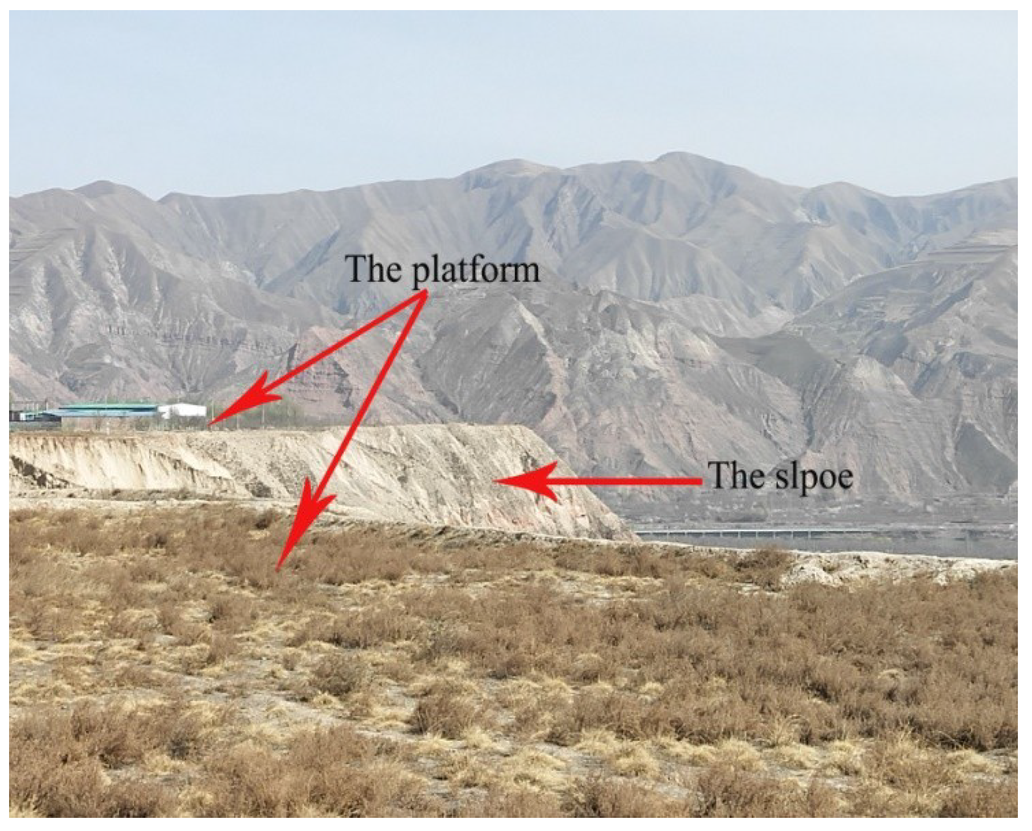
The South Jingyang Platform is located between the city of Xianyang and Jingyang country, with an area of about 70 km2. The elevation difference between the top and bottom of the platform varies from about 50 to 100 m and its slope ranges from 40° to 90° (Figure 1). The angle of the upper part of the slope is approximately 60° with a height difference of 10–15 m and the angle of the lower slope is approximately 50° with a height difference of 40–80 m. Malan loess (Q3 loess) and Lishi loess (Q2 loess) are the main constituents of the carcass. In the study area, the typical loess irrigated area of Shutangwang Village was selected (the geographical coordinates are 108.84° E, 34.49° N) for the field irrigation infiltration test and the acquisition of the indoor experiment soil samples.
2.1.2. The Field Irrigation Experiment
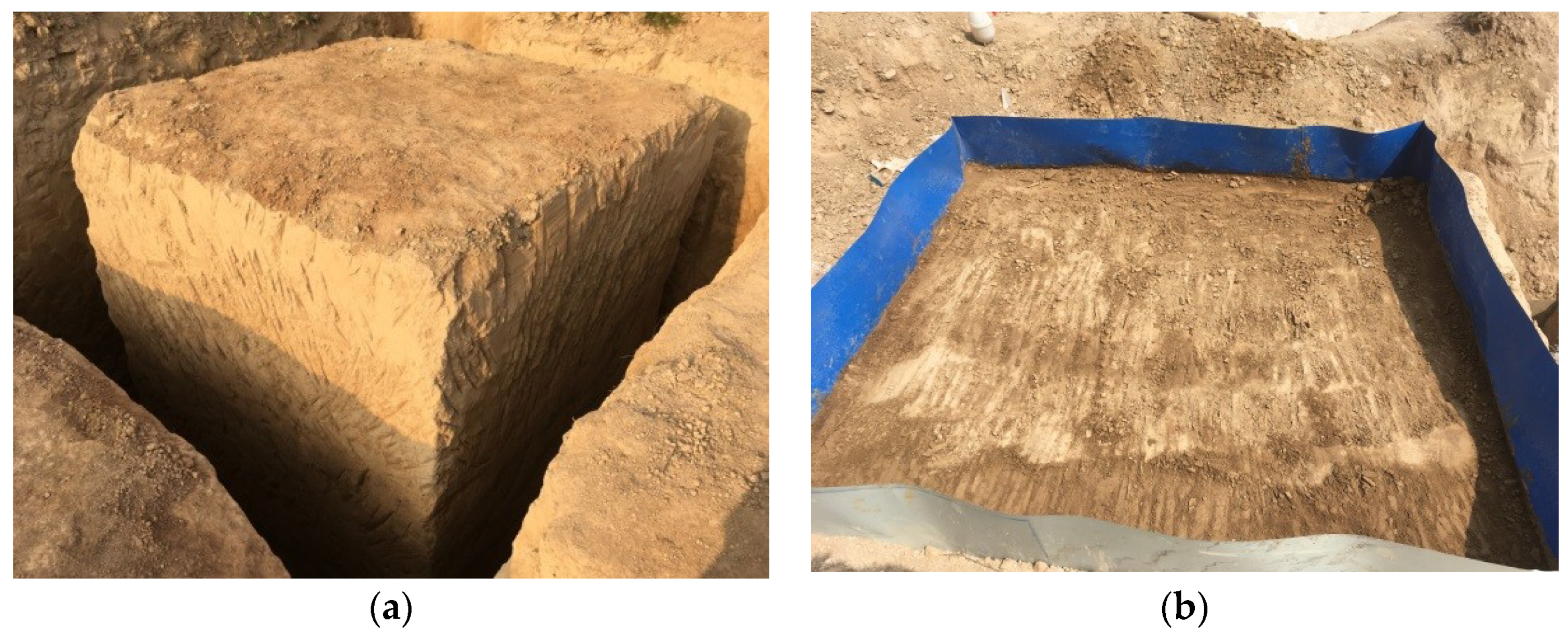
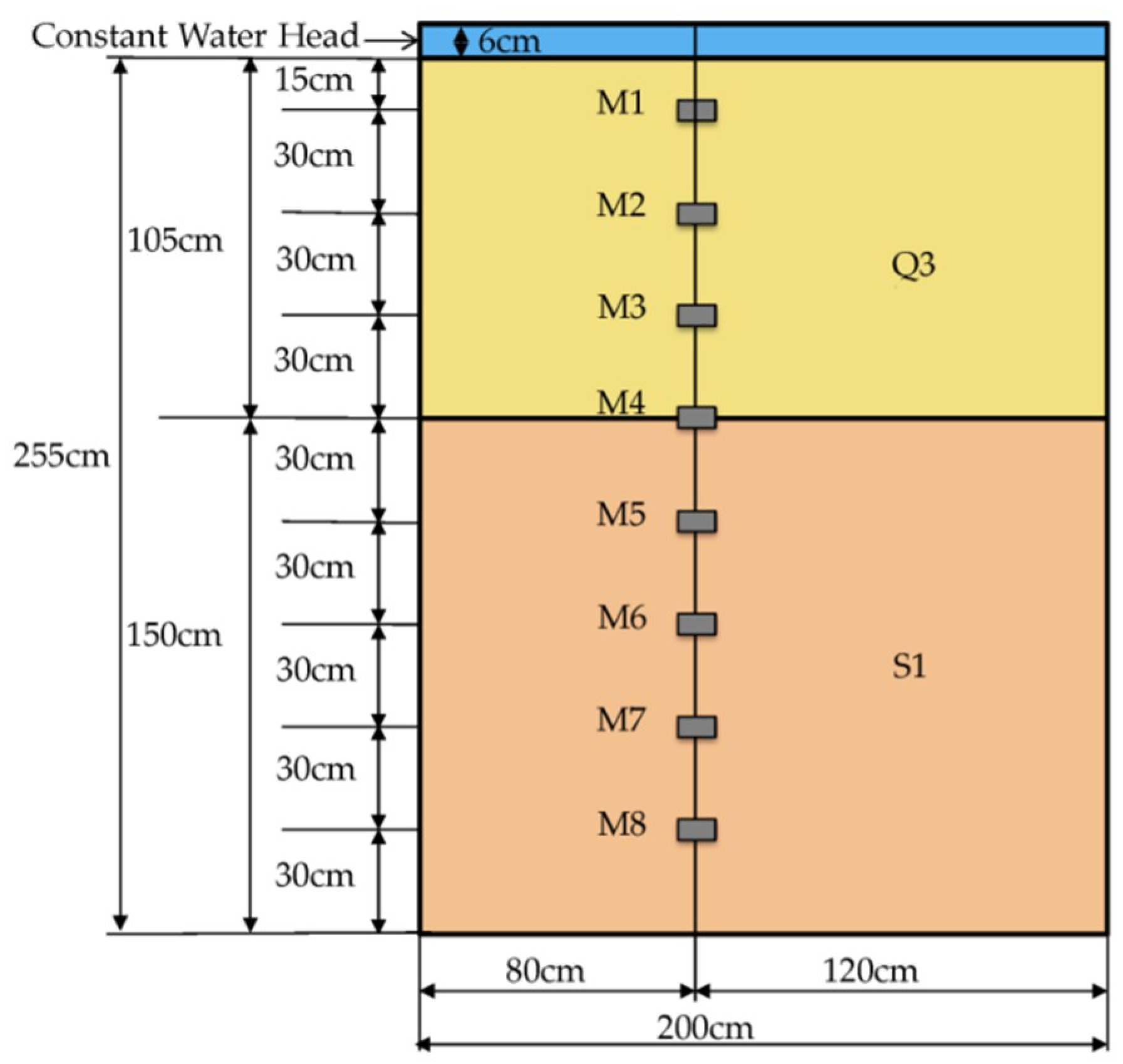
The purpose of this field experiment was to observe the water infiltration process under the irrigation condition. As shown in Figure 2a, we manually excavated the soil column with 200 cm in both length and width and 255 cm in height, sealed the surrounding of the soil column with bentonite and wrapped plastic film around the soil. One vertical side of the soil column was left uncovered to embed the sensors. The soil column was combined with two different soils, the upper 105 cm Q3 loess and the lower 150 cm S1 palaeosol. As shown in Figure 3, 8 Time-Domain Reflectometry (TDR)-3 moisture sensors were embedded along the depth of the soil column and the corresponding depth was 15 cm, 45 cm, 75 cm, 105 cm, 135 cm, 165 cm, 195 cm, 225 cm from the top surface of the soil column. We connected the installed sensors to the CR3000 data logger, backfilled the sensor holes with bentonite, and finally sealed the boundary with bentonite. Figure 2b shows a water retaining plate arranged above the soil column to provide a 6 cm constant head boundary condition during the irrigation process. The data logger acquisition interval was 3 min in order to achieve continuous, real-time observations of the entire process of irrigation. The irrigation test stopped when the moisture sensor at the 2.25 m depth responded, which happened after 58.65 h.
2.1.3. Large Laboratory Soil Column Infiltration Experiment
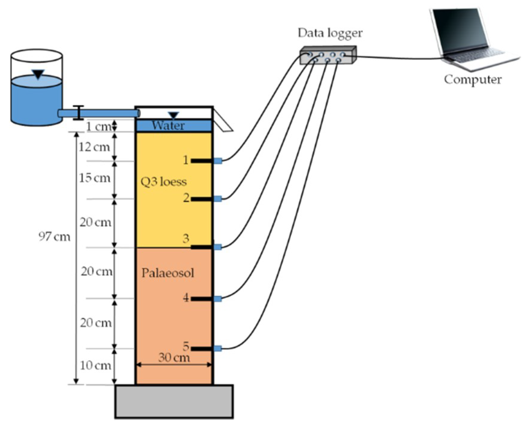
The undisturbed loess column was collected by carefully introducing a rigid polyvinyl chloride (PVC) cylinder into the soil. The PVC cylinder was 100 cm in height and 30 cm in inner diameter, with a wall thickness of 1 cm. The specific sampling process was as follows: first, the soil around the target location was excavated and slowly the upper part of the clod reserved in the middle was cut into a small size that was the same as the inner diameter of the cylinder; second, the cylinder was placed on the top of the clod and the cylinder was slightly pressed to place the undisturbed soil within it; third, a spatula was used to cut the next soil section and the cylinder pressed again until the soil reached the top of it; finally, the soil column was shovelled from the root to obtain the undisturbed soil column for the laboratory infiltration experiment. Note that the inner wall of the PVC cylinder was coated with Vaseline to ensure close contact with the soil to prevent preferential flow during the experimental procedure. During the soil column excavation procedure, the undisturbed small soil samples were obtained to satisfy the requirement of the hydraulic experiments in the laboratory.
We removed 3 cm of soil from the top of the column, leaving 47 cm of loess and 50 cm of palaeosol, to eliminate the influence of the disturbed soil. In addition, a sheet of filter paper and a permeable stone were placed at the bottom of the soil column. Afterwards, the soil column was placed on the base, which had a hole in the centre for water drainage or air expulsion. We sealed the gap between the side wall of the PVC cylinder and the base with glass glue to ensure that no water flowed out from here during the test. As shown in Figure 4, the soil column was equipped with five tensiometers (T1 to T5), installed at the corresponding reserved holes 12, 27, 47, 67, and 87 cm from the top of the soil column, respectively. A sheet of filter paper was placed on the top of the soil specimen to avoid disturbing the soil sample during the test. The water supply container was connected and an overflow hole was provided 2 cm from the top of the PVC cylinder to maintain a 1 cm constant water head. The tensiometers were connected to the CR3000 data logger and we observed the corresponding readings using a computer to judge whether the test device was normal. The data acquisition interval was 1 min. The experiment ended when the response of the fifth tensiometer was terminated, which was after 575 min. All sensors responded well.
2.1.4. Test of the Basic Physical and Hydraulic Properties of the Study Soil
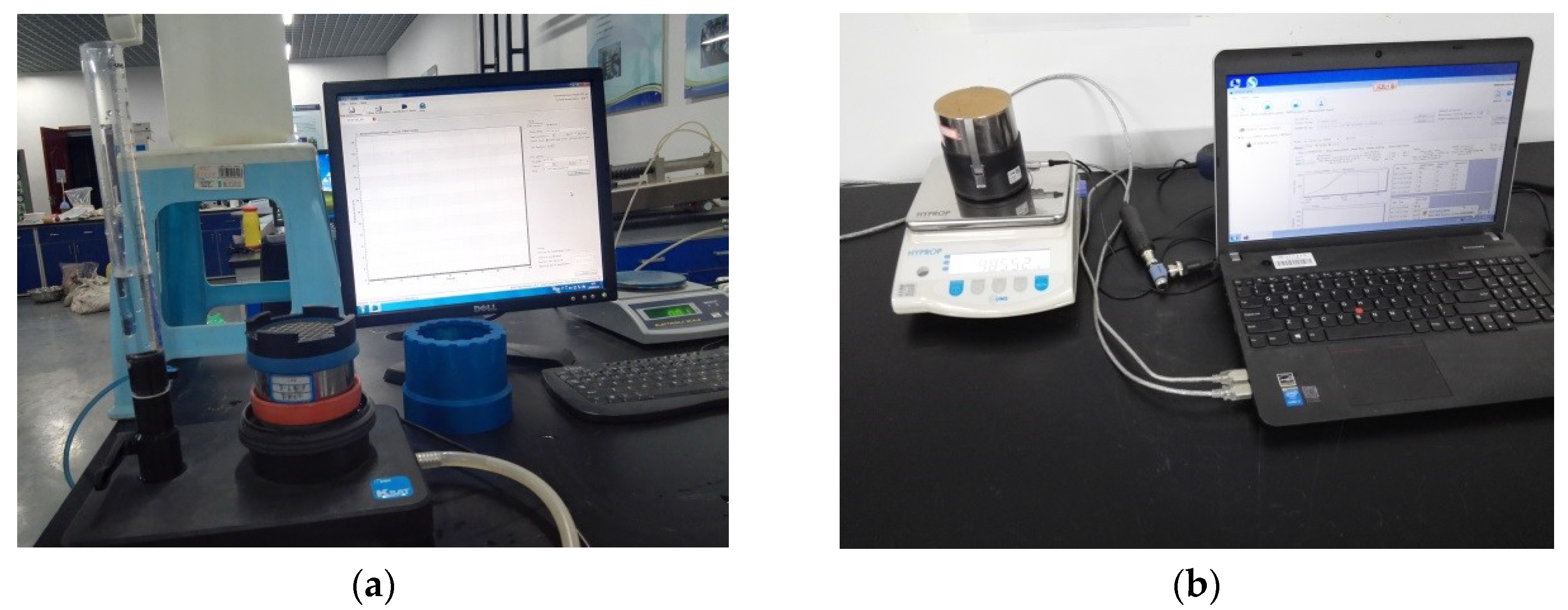
A Bettersize 2000 laser particle size analyser (Dandong Better Instrument Corporation, Dandong, China) was applied to determine the grain size distribution of the soil, which is shown in Table 1. We used the HYPROP device and the Ksat device produced by the Universiti Malaysia Sabah (UMS) Company in Germany to obtain the SWCC and the saturated hydraulic conductivity, respectively (Figure 5). The saturated hydraulic conductivity of the loess was 1.33 × m/s, which was larger than that of the palaeosol (1.19 × m/s).
2.2. Theory of the Soil Hydraulic Properties
2.2.1. Infiltration Model of the Layered Soil
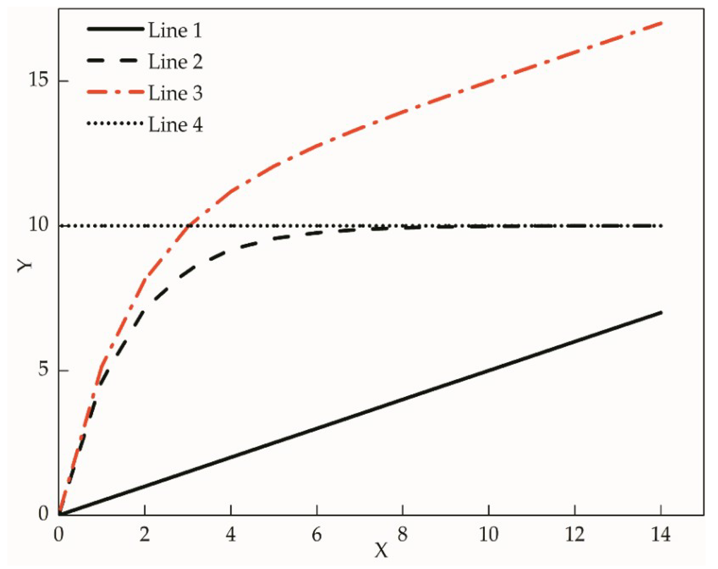
The relationship between the cumulative infiltration and time for layered soils can be expressed by piecewise formulas, meaning that the nonlinear section is simulated by existing models for homogeneous soils and the linear section is simulated by a linear equation. It is important to determine the stable infiltration rate and the transition time in this method. A large number of experimental and theoretical analyses have proven that the infiltration transition of layered soil from a nonlinear process to a linear process exists [18]. The infiltration process of the upper soil layer can be seen as a superposition of two parts. One part is a stable infiltration. The other part can be regarded as a flushing process, which can be described by the exponential relationship using Equation (1). The cumulative infiltration is the superposition of the flushing process and the stable infiltration [33].The schematic diagram of the proposed model is shown below:
As can be seen from Figure 6, Line 1 is a linear model and Line 2 is a nonlinear model. Line 3 is a superposition model of Line 1 and Line 2, and Line 4 is an asymptote of Line 2. The model form of Line 2 is:
where is the value of the asymptote of Line 2, which is the value of Line 4; is the time constant, which is generally 1/3 of the transition time. For the infiltration problem of layered soils, the water flushing process of the upper soil layer adopts the relationship of the Equation (1), and the stable infiltration part is simulated by the relationship of the Line 1. It can be seen from Figure 6 that the value of the Line 2 no longer increases after the transition time and the infiltration process becomes linear. The infiltration model can be obtained:
where I is the cumulative infiltration (cm); is the steady infiltration rate (cm ), determined by the test data fitting; t is the time (min); is the intercept of the linear part and the vertical axis (cm), and the value can also be determined by fitting; τ is the turning time constant (min); is the infiltration rate (cm ).
2.2.2. Description of the Basic Soil Hydraulic Properties
SWCC defines the functional relationship between pressure head and soil water content. Many empirical formulas have been proposed to describe SWCC, such as the Brooks–Corey, Gardner, van Genuchten (VG), and Gardner–Russo models. In this paper, we used the VG model to fit the experimental data and used Origin 9.1 software to fit the model parameters. In this study, HYDRUS-1D software was used to calculate the forward model. We adopted the Bayesian approach and quantified parameter uncertainty using the DREAM(zs) algorithm. Time series of the pressure head measured at five different depths of the laboratory soil column were used for soil hydraulic parameter inversion. In the Bayesian framework, the parameter posterior distribution p (m|) can be derived from the experimental data using Bayes’ law, as follows:
where p (m) is the prior distribution of the parameter vector m, L (m|) ≡ p (|m) is the likelihood function that summarizes the level of agreement between the observed and simulated data, and is the normalized constant of the probability density function. We resorted to the efficient DREAM(zs) algorithm to numerically estimate the posterior distribution p (m|). The DREAM(zs) algorithm includes various statistical tests to determine when the convergence of the sampled chains to a limiting distribution has been achieved. The most powerful convergence test is the multi-chain -statistic [34]. The convergence exactly occurs as soon as the -statistic decreases to less than the critical threshold 1.2 for all the parameters of the target distribution; otherwise, one should increase the number of iterations and the chains run for a longer period.
3. Results and Discussion
3.1. The Field Infiltration Experiment
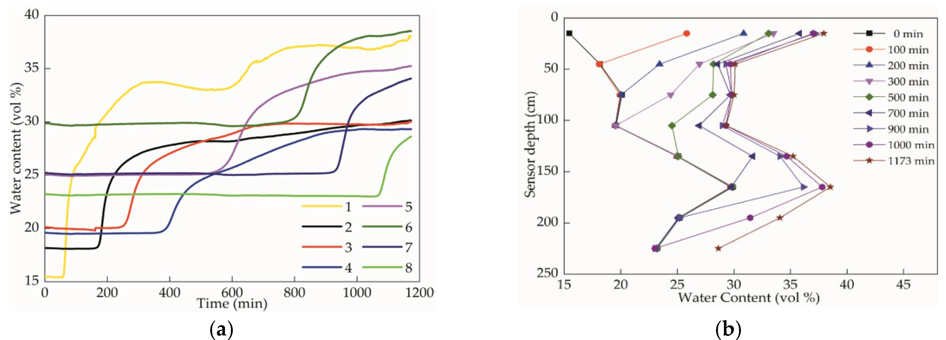
Figure 7a shows that soil water content at the position of moisture sensors 1–8 changed with the irrigation time. The variation in soil water content experienced four stages: stable state, sharply rising state, slowly rising, and stable state again. Figure 7b shows that when the saturated zone of the loess reached a certain depth, it would not move down. The water migrated downward in the unsaturated state in the soil, so the actual migration form of water in the loess was dominated by unsaturated forms. At the same time, Figure 7 and Table 2 demonstrate that the water content of the palaeosol was significantly greater than that of the loess, which could be explained by the high content of clay in palaeosol soil. This is consistent with the conclusion in [8]. Figure 7b shows that the water content above and below the position of sensor 4 was discontinuous. From the perspective of energy, when the water moves from one layer to another, the water potential at the interface should be continuous, inevitably causing the soil moisture in the upper and lower layers of the interface to be discontinuous.
3.2. Laboratory Soil Column Infiltration Experiment Results
3.2.1. Variance of the Matric Suction during the Infiltration Process
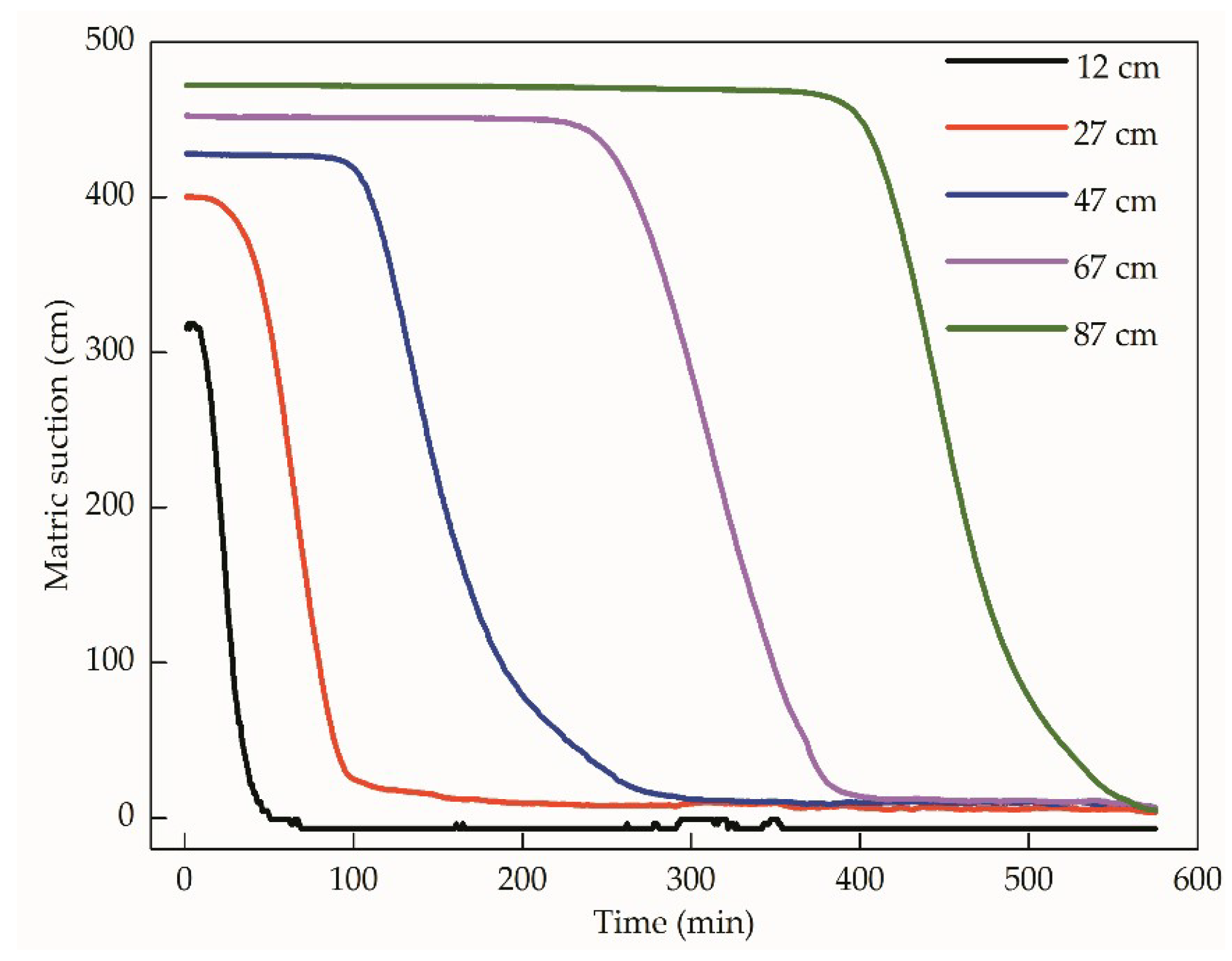
As we can see from Figure 8, the changes in the matric suction were divided into three stages, as follows: stable before the wetting front arrived, sharply decreasing when the wetting front arrived, and basically stable after a period of time. The matric suction values were relatively high for all sensors during the initial stage of the infiltration. When the wetting front arrived, the infiltration capacity of the soil was high and the matric suction rapidly decreased. As time passed, the decreasing rate of the matric suction slowed. After a certain period of time, the soil matric suction was stable. Comparatively speaking, the closer the tensiometer was to the top surface, the faster the suction changed. It can be seen from the figure that the migration velocity of the wetting front below 47 cm was significantly slowed down, which indicates that the infiltration rate of water in the lower layer of palaeosol was reduced.
3.2.2. Infiltration Models
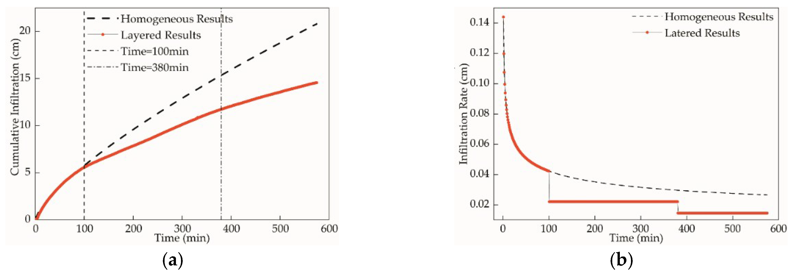
The studied layered soil was the combination of the upper Q3 loess and the lower S1 palaeosol, and the infiltration test lasted for 575 min. Before the wetting front reached the interface between loess and palaeosol (t 100 min), the change process of cumulative infiltration with time was the same as that of the homogeneous soil. The relationship between the cumulative infiltration and the time was nonlinear, which can be simulated by Kostiakov’s infiltration model, as follows:
where I is the cumulative infiltration amount (cm), t is the time (min), and is the relationship coefficient.
When the wetting front reached the interface between the two soils (t 100 min), the infiltration process was obviously slow and the cumulative infiltration showed a significant transition. The relationship between cumulative infiltration and time changed from a nonlinear process to a linear process, indicating that the infiltration process became stable. The test data after the transition was fitted by a linear relationship, yielding the following formula:
where I is the cumulative infiltration amount (cm) and t is the infiltration time (min).
The relationship between the infiltration rate and time can be obtained from the derivation of the relationship between the cumulative infiltration amount and time over time. The relationship between soil infiltration rate and time in the upper part of the layered soil can be expressed by the following formula:
where is the infiltration rate.
The variation in soil infiltration rate with time is shown in Figure 9b. The infiltration rate of the layered soil was the same as that of the homogeneous soil before the wetting front reached the lower layer. After the wetting front entered the lower layer, the infiltration rate became constant, that is, the infiltration turned into a stable process. There were two different linear parts, 0.0221 cm/min and 0.0145 cm/min, meaning that the infiltration rate reduced again at t = 380 min when the wetting front reached the fifth sensor, for the reason that the palaeosol under the fifth sensor had many calcareous concretions and stronger water resistance. According to the variation characteristics of the infiltration rate, the whole infiltration process of the layered soils can be divided into nonlinear and linear stages. Moreover, the infiltration rates of stable states were significantly smaller than the instantaneous infiltration rate of homogeneous soil at the transition time . This phenomenon fully illustrates the anti-seepage effect of layered soil, which is consistent with [18,22].
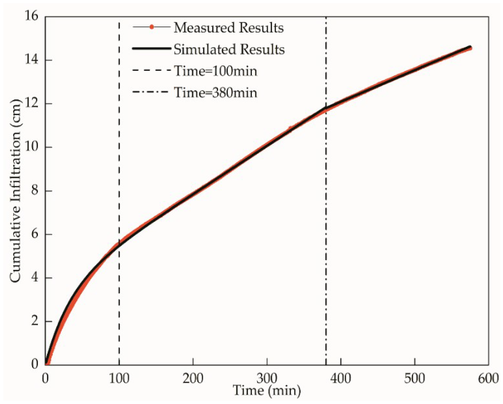
According to Equation (2), we can describe the cumulative infiltration as follows:
It can be seen from Figure 10 that both the calculated values and the measured values are in good agreement. The layered soil infiltration model established by superposition principle can simulate the layered soil infiltration well. That is to say, the cumulative infiltration could be divided into the flushing process and the stable infiltration process before the wetting front arrived at the interface between the two soils. The cumulative infiltration became stable, with an infiltration rate smaller than that of the homogeneous soil under the same situation.
3.3. The Basic Physical and Hydraulic Properties
3.3.1. Laboratory SWCC Experiments
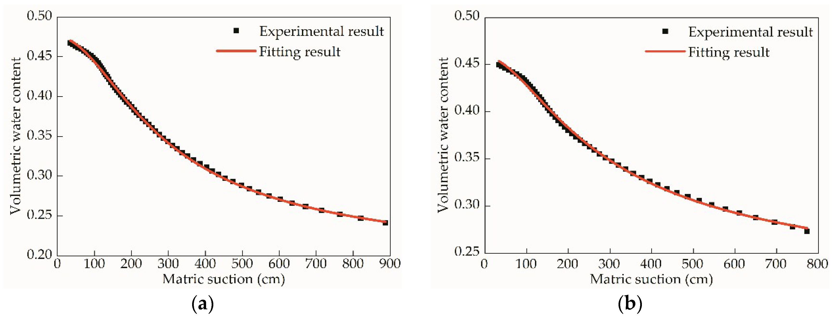
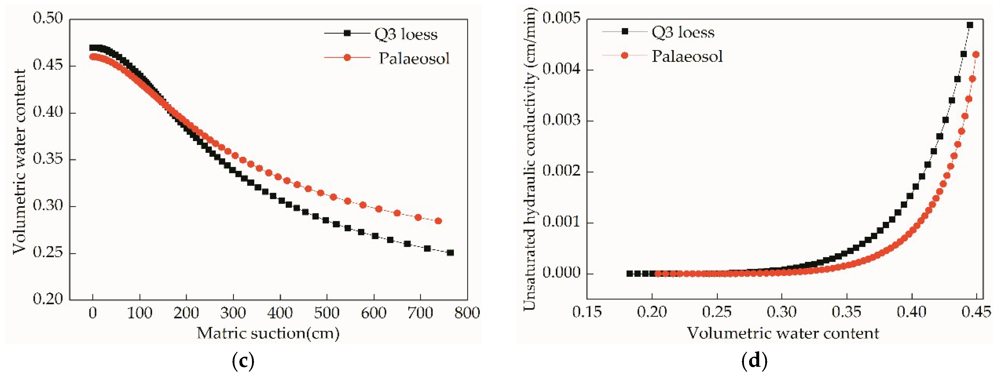
As shown in Figure 11a,b, the values of the correlation coefficient () of the fitting were 0.999 for the loess and 0.998 for the palaeosol, indicating that the laboratory results agree well with the VG model. Figure 11c indicates that the SWCCs of the loess and palaeosol intersect with each other at a suction value of approximately 155 cm, meaning that the water holding capacity of the loess layer was stronger than that of the palaeosol layer in the lower matric suction range and was weaker than that of the palaeosol layer when the matric suction was greater than 155 cm. We can see from Figure 11d that the unsaturated hydraulic conductivity of the loess and palaeosol was very low when volumetric water content was less than 0.3. The unsaturated hydraulic conductivity rapidly increased to the saturated hydraulic conductivity with the increase in volumetric water content when the volumetric water content was greater than 0.3. Furthermore, the unsaturated hydraulic conductivity of the loess was always higher than that of the palaeosol under the same volumetric water content.
Table 1 shows that the content of silt was higher than that of clay for both soils, which is consistent with the results of previous studies [22]. However, the loess had a higher quantity of coarse silt and a lower quantity of fine silt and clay than the palaeosol. The main reason is the difference in the pedogenesis due to different climates. That is, palaeosol developed in warmer/wetter climatic conditions was subjected to stronger pedogenesis than the loess, which was deposited during colder/drier times. As a result, the loess layer had a stronger water holding capacity than the palaeosol layer had in the lower suction section, and the water holding capacity of the loess was less than the palaeosol layer had in the higher suction section, as shown in Figure 11c. Moreover, water adsorption by clay also explains why the water holding capacity of the palaeosol was stronger than that of the loess in the higher suction section.
Combining the results of Figure 11c,d, we can conclude that when the water enters the palaeosol from the loess, the suction of the palaeosol is greater than that of the loess and the wetting front directly enters the palaeosol. That is to say, the infiltration of the lower palaeosol layer is less affected by the infiltration of the upper loess layer. The water-blocking effect of palaeosol is mainly due to the fact that the hydraulic conductivity of palaeosol is lower than that of loess. After the infiltrated water reaches the lower soil, the water supply from the upper layer soil is greater than the soil hydraulic conductivity of the lower layer soil and the infiltration is under the condition of sufficient water for the lower layer soil. Therefore, excess water may accumulate above the interface between the upper and lower soil layers and gradually generate temporary groundwater levels, which is consistent with [22].
3.3.2. Inverse Simulation Results of the DREAM Algorithm
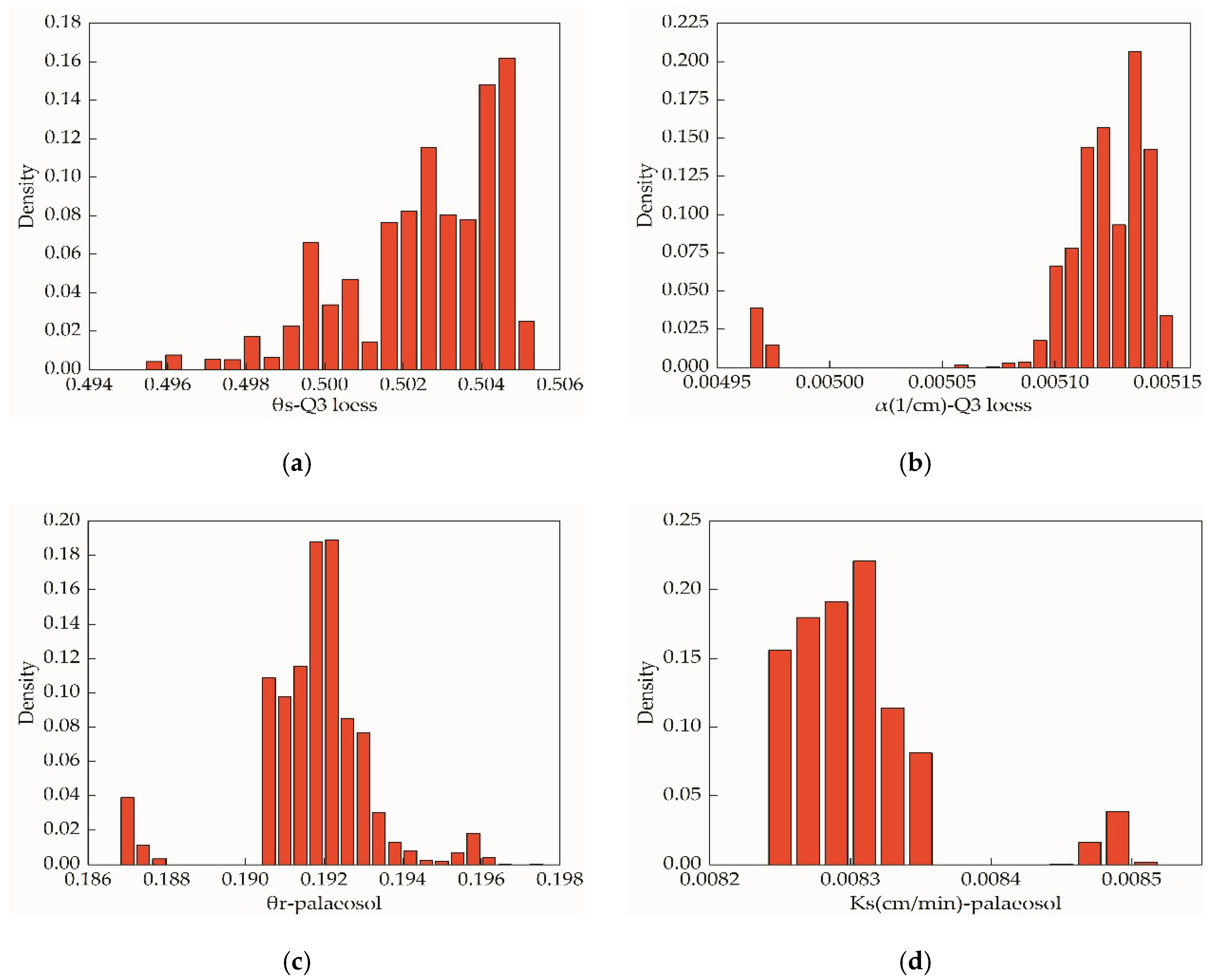
The posterior probability density distributions of the soil hydraulic parameters were estimated using the Bayesian simulation with the DREAM(zs) algorithm. The parameters’ convergence was tested by the multi-chain -statistic method mentioned above. As shown in Figure 12, the posterior probability distributions are skewed and the peak values are obvious, indicating that the parameter identification is good and the uncertainty is relatively small. The posterior probability distributions are irregular and some of the highest are the maximum or minimum values at the boundary of the parameter ranges. The parameter values derived from the fitting results are near the ranges of the posterior distribution. However, differences remain between them. The main reasons are the hysteretic effect and the size effect. Numerical models neglecting these differences may compromise the reliability of the predictions and misrepresent the responses. However, the fitting parameters can provide a reference for a decision of initial prior ranges in the MCMC optimization algorithm. In addition, the distinct multiple frontal distribution of the posterior distribution of some parameters means that there may be more than one optimal solution. Therefore, the MCMC algorithm can effectively avoid the problem of obtaining a local optimal solution.
4. Conclusions
Large soil column infiltration experiments under a constant water head were conducted on both laboratory and field scales to simulate the water infiltration process under agricultural irrigation. The hydraulic property differences between the Q3 loess and palaeosol were analysed by comparing the basic hydraulic parameters. The main conclusions of this paper are:
- According to the comparison of SWCC between loess and palaeosol, the water holding capacity of palaeosol is stronger than that of loess under the same matrix suction. Therefore, the water content of palaeosol is always higher than that of loess at the beginning and ending of the field test. The loess does not weaken the infiltration of the palaeosol. The reason for the water-resistance of the palaeosol is that its unsaturated hydraulic conductivity is lower than that of loess, which also leads to the appearance of a temporary water table at the interface between loess and palaeosol under certain infiltration conditions.
- In the laboratory infiltration test, before the wetting front reached the interface between loess and palaeosol, the relationship between the cumulative infiltration and time was nonlinear, which is consistent with that of homogeneous soil. However, after the wetting front reaches the interface, the relationship between the cumulative infiltration and time became linear. The superposition model based on the capacitance law can continuously simulate the nonlinear and linear relationships between the cumulative infiltration and time well.
- The water infiltration simulation experiments with two different scales illustrated that the process of water content change in the layered loess–palaeosol sequence can be divided into two stages: the first stage is the free infiltration stage of the loess under the constant water head; the second stage is the free infiltration stage of the palaeosol under the variable water head.
Author Contributions
Conceptualization, F.D.; Data curation, Q.G. and Z.Z.; Formal analysis, Q.G.; Funding acquisition, F.D.; Methodology, F.D.; Project administration, F.D.; Writing—Original draft, Q.G.; Writing—Review and Editing, Q.G. and F.D.
Funding
This research was funded by National Basic Research Program of China, grant number 2014CB744700.
Acknowledgments
We thank Renchao Li for English language editing.
Conflicts of Interest
The authors declare no conflict of interest.
References
- Peng, J.B.; Wang, G.H.; Wang, Q.Y.; Zhang, F.Y. Shear wave velocity imaging of landslide debris deposited on an erodible bed and possible movement mechanism for a loess landslide in Jingyang, Xi’an, China. Landslides 2017, 14, 1503–1512. [Google Scholar] [CrossRef]
- Leng, Y.Q.; Peng, J.B.; Wang, Q.Y.; Meng, Z.J.; Huang, W.L. A fluidized landslide occurred in the Loess Plateau: A study on loess landslide in South Jingyang tableland. Eng. Geol. 2018, 236, 129–136. [Google Scholar] [CrossRef]
- Zhuang, J.Q.; Peng, J.B.; Wang, G.H.; Javed, I.; Wang, Y.; Li, W. Distribution and characteristics of landslide in Loess Plateau: A case study in Shaanxi province. Eng. Geol. 2018, 236, 89–96. [Google Scholar] [CrossRef]
- Xu, L.; Dai, F.C.; Tham, L.G.; Tu, X.B.; Min, H.; Zhou, Y.F.; Wu, C.X.; Xu, K. Field testing of irrigation effects on the stability of a cliff edge in loess, North-west China. Eng. Geol. 2011, 120, 10–17. [Google Scholar] [CrossRef]
- Xu, L.; Dai, F.C.; Tu, X.B.; Tham, L.G.; Zhou, Y.F.; Iqbal, J. Landslides in a loess platform, North-West China. Landslides 2014, 11, 993–1005. [Google Scholar] [CrossRef]
- Zhuang, J.Q.; Peng, J.B. A coupled slope cutting—A prolonged rainfall-induced loess landslide: A 17 October 2011 case study. Bull. Eng. Geol. Environ. 2014, 73, 997–1011. [Google Scholar] [CrossRef]
- Wang, H.F.; Wang, M.Y. Infiltration experiments in layered structures of upper porous and lower fractured media. J. Earth Sci. 2013, 24, 843–853. [Google Scholar] [CrossRef]
- Zhao, P.P.; Shao, M.A.; Melegy, A.A. Soil Water Distribution and Movement in Layered Soils of a Dam Farmland. Water Resour. Manag. 2010, 24, 3871–3883. [Google Scholar] [CrossRef]
- Samani, Z.; Cheraghi, A.; Willardson, L. Water Movement in Horizontal Layered Soils. J. Irrig. Drain. Eng. 1989, 115, 449–456. [Google Scholar] [CrossRef]
- Li, J.S.; Ji, H.Y.; Li, B.; Liu, Y.C. Wetting Patterns and Nitrate Distributions in Layered-Textural Soils under Drip Irrigation. Agric. Sci. China 2007, 6, 970–980. [Google Scholar] [CrossRef]
- Yang, H.; Rahardjo, H.; Leong, E.C. Behavior of Unsaturated Layered Soil Columns during Infiltration. J. Hydrol. Eng. 2006, 11, 329–337. [Google Scholar] [CrossRef]
- Wang, T.T.; Catherine, E.S.; Ma, J.B.; Zheng, J.Y.; Zhang, X.C. Applicability of five models to simulate water infiltration into soil with added biochar. J. Arid Land 2017, 9, 701–711. [Google Scholar] [CrossRef]
- Dashtaki, S.G.; Homaee, M.; Mahdian, M.H.; Kouchakzadeh, M. Site-Dependence Performance of Infiltration Models. Water Resour. Manag. 2009, 23, 2777–2790. [Google Scholar] [CrossRef]
- Chu, X.F.; Mariño, M.A. Determination of ponding condition and infiltration into layered soils under unsteady rainfall. J. Hydrol. 2005, 313, 195–207. [Google Scholar] [CrossRef]
- Sakellario-Makrantonaki, M. Water Drainage in Layered Soils. Laboratory Experiments and Numerical Simulation. Water Resour. Manag. 1997, 11, 437–444. [Google Scholar] [CrossRef]
- Ma, Y.; Feng, S.Y.; Su, D.Y.; Gao, G.Y.; Huo, Z.L. Modeling water infiltration in a large layered soil column with a modified Green–Ampt model and HYDRUS-1D. Comput. Electron. Agric. 2010, 71, 40–47. [Google Scholar] [CrossRef]
- Corradini, C.; Morbidelli, R.; Flammini, A.; Govindaraju, R.S. A parameterized model for local infiltration in two-layered soils with a more permeable upper layer. J. Hydrol. 2011, 396, 221–231. [Google Scholar] [CrossRef]
- Mohammadzadeh-Habili, J.; Heidarpour, M. Application of the Green-Ampt model for infiltration into layered soils. J. Hydrol. 2015, 527, 824–832. [Google Scholar] [CrossRef]
- Al-Maktoumi, A.; Kacimov, A.; Al-Ismaily, S.; Al-Busaidi, H.; Al-Saqri, S. Infiltration into Two-Layered Soil: The Green–Ampt and Averyanov Models Revisited. Transp. Porous Media 2015, 109, 169–193. [Google Scholar] [CrossRef]
- Ma, Y.; Feng, S.Y.; Zhan, H.B.; Liu, X.D.; Su, D.Y.; Kang, S.Z.; Song, X.F. Water Infiltration in Layered Soils with Air Entrapment: Modified Green-Ampt Model and Experimental Validation. J. Hydrol. Eng. 2011, 16, 628–638. [Google Scholar] [CrossRef]
- Zhao, J.B.; Long, T.W.; Wang, C.Y.; Zhang, Y. How the Quaternary climatic change affects present hydrogeological system on the Chinese Loess Plateau: A case study into vertical variation of permeability of the loess-palaeosol sequence. Catena 2012, 92, 179–185. [Google Scholar] [CrossRef]
- Zhao, J.B.; Ma, Y.D.; Cao, J.J.; Wei, J.P.; Shao, T.J. Effect of Quaternary climatic change on modern hydrological systems in the southern Chinese Loess Plateau. Environ. Earth Sci. 2015, 73, 1161–1167. [Google Scholar] [CrossRef]
- Ekblad, J.; Isacsson, U. Time-domain reflectometry measurements and soil-water characteristic curves of coarse granular materials used in road pavements. Can. Geotech. J. 2007, 44, 858–872. [Google Scholar] [CrossRef]
- Tarantino, A.; Ridley, A.M.; Toll, D.G. Field Measurement of Suction, Water Content, and Water Permeability. Geotech. Geol. Eng. 2008, 26, 751–782. [Google Scholar] [CrossRef]
- Godoy, V.A.; Zuquette, L.V.; Gómez-Hernández, J.J. Scale effect on hydraulic conductivity and solute transport: Small and large-scale laboratory experiments and field experiments. Eng. Geol. 2018, 243, 196–205. [Google Scholar] [CrossRef]
- Scharnagl, B.; Vrugt, J.A.; Vereecken, H.; Herbst, M. Inverse modelling of in situ soil water dynamics: Investigating the effect of different prior distributions of the soil hydraulic parameters. Hydrol. Earth Syst. Sci. 2011, 15, 3043–3059. [Google Scholar] [CrossRef]
- Li, B.L.; Liu, Y.; Nie, W.B.; Ma, X.Y. Inverse Modeling of Soil Hydraulic Parameters Based on a Hybrid of Vector-Evaluated Genetic Algorithm and Particle Swarm Optimization. Water 2018, 10, 84. [Google Scholar] [CrossRef]
- Sen, M.K.; Stoffa, P.L. Bayesian inference, Gibbs’ sampler and uncertainty estimation in geophysical inversion. Geophys. Prospect. 1996, 44, 313–350. [Google Scholar] [CrossRef]
- Vrugt, J.A.; Ter Braak, C.J.F.; Diks, C.G.H.; Robinson, B.A.; Hyman, J.M.; Higdon, D. Accelerating Markov Chain Monte Carlo Simulation by Differential Evolution with Self-Adaptive Randomized Subspace Sampling. Int. J. Nonlinear Sci. Numer. Simul. 2009, 10, 273–290. [Google Scholar] [CrossRef]
- Qin, H.; Xie, X.Y.; Vrugt, J.A.; Zeng, K.; Hong, G. Underground structure defect detection and reconstruction using crosshole GPR and Bayesian waveform inversion. Autom. Constr. 2016, 68, 156–169. [Google Scholar] [CrossRef] [Green Version]
- Liu, W.P.; Luo, X.Y.; Huang, F.; Fu, M.F. Uncertainty of the Soil–Water Characteristic Curve and Its Effects on Slope Seepage and Stability Analysis under Conditions of Rainfall Using the Markov Chain Monte Carlo Method. Water 2017, 9, 758. [Google Scholar] [CrossRef]
- Vrugt, J.A. Markov chain Monte Carlo simulation using the DREAM software package: Theory, concepts, and MATLAB implementation. Environ. Model. Softw. 2016, 75, 273–316. [Google Scholar] [CrossRef] [Green Version]
- Zhang, J.P. Experimental Study on Infiltration Characteristics and Finger Flow in Layer Soils of the Loess Area. Ph.D. Thesis, Northwest Sci-Tech University of Agriculture and Forestry, Yangling, China, 2004. [Google Scholar]
- Gelman, A.; Rubin, D.B. Inference from Iterative Simulation Using Multiple Sequences. Stat. Sci. 1992, 7, 457–511. [Google Scholar] [CrossRef]
Figure 1.
The topographic features of the studied area.

Figure 2.
Field infiltration experiment: (a) the field soil column; (b) water retaining plate at the surface of the soil column.
Figure 2.
Field infiltration experiment: (a) the field soil column; (b) water retaining plate at the surface of the soil column.

Figure 3.
Diagram of the field soil column infiltration experiment.

Figure 4.
Diagram of the laboratory soil column infiltration experiment.

Figure 5.
The devices for the basic hydraulic properties: (a) the Ksat device; (b) the HYPROP device.
Figure 5.
The devices for the basic hydraulic properties: (a) the Ksat device; (b) the HYPROP device.

Figure 6.
The schematic diagram of the overlay model.

Figure 7.
The field experiment results: (a) the variance of the volumetric water content with time; (b) water content isochrones.
Figure 7.
The field experiment results: (a) the variance of the volumetric water content with time; (b) water content isochrones.

Figure 8.
Variance in the matric suction with time at different depths.

Figure 9.
The variance of the cumulative infiltration and infiltration rate: (a) the relationship between the cumulative infiltration and time; (b) the relationship between the infiltration rate and time.
Figure 9.
The variance of the cumulative infiltration and infiltration rate: (a) the relationship between the cumulative infiltration and time; (b) the relationship between the infiltration rate and time.

Figure 10.
Simulation effect of continuous function infiltration model.

Figure 11.
The basic hydraulic properties: (a) the fitting of the loess SWCC; (b) the fitting of the palaeosol SWCC; (c) the SWCC comparison between the two different soils; (d) the comparison of the hydraulic conductivity between the two different soils.
Figure 11.
The basic hydraulic properties: (a) the fitting of the loess SWCC; (b) the fitting of the palaeosol SWCC; (c) the SWCC comparison between the two different soils; (d) the comparison of the hydraulic conductivity between the two different soils.


Figure 12.
Histograms of the parameter posterior distribution derived from DREAM(zs) algorithm: (a) saturated volumetric water content of the Q3 loess (; (b) empirical parameters of the Q3 loess (); (c) residual volumetric water content of the palaeosol (); and (d) saturated hydraulic conductivity of the palaeosol (cm ).


Table 1.
Grain size distribution.
| Granular Group (Particle Size Range) | Content Ratio (%) | ||
|---|---|---|---|
| Q3 Loess Palaeosol | |||
| Sand (0.05–2 mm) | 3.91 | 8.95 | |
| Silt (0.005–0.05 mm) | Coarse silt (0.01–0.05 mm) | 67.88 | 56.57 |
| Fine silt (0.005–0.01 mm) | 1.76 | 2.78 | |
| Clay 0.005 mm) | 31.7 | ||
Table 2.
The measured water contents at the start and end of the measurement (%).
| Sensor Number | 1 | 2 | 3 | 4 | 5 | 6 | 7 | 8 |
|---|---|---|---|---|---|---|---|---|
| T = 0 h | 15 | 18 | 20 | 20 | 25 | 30 | 25 | 23 |
| T = 58.65 h | 38 | 31 | 30 | 29 | 35 | 39 | 34 | 29 |
© 2019 by the authors. Licensee MDPI, Basel, Switzerland. This article is an open access article distributed under the terms and conditions of the Creative Commons Attribution (CC BY) license (http://creativecommons.org/licenses/by/4.0/).
Share and Cite
MDPI and ACS Style
Guo, Q.; Dai, F.; Zhao, Z. Analysis of the Hydraulic Properties of Undisturbed Layered Loess in Northwest China. Water 2019, 11, 1379. https://doi.org/10.3390/w11071379
AMA Style
Guo Q, Dai F, Zhao Z. Analysis of the Hydraulic Properties of Undisturbed Layered Loess in Northwest China. Water. 2019; 11(7):1379. https://doi.org/10.3390/w11071379
Chicago/Turabian StyleGuo, Qinghua, Fuchu Dai, and Zhiqiang Zhao. 2019. "Analysis of the Hydraulic Properties of Undisturbed Layered Loess in Northwest China" Water 11, no. 7: 1379. https://doi.org/10.3390/w11071379
Note that from the first issue of 2016, this journal uses article numbers instead of page numbers. See further details here.