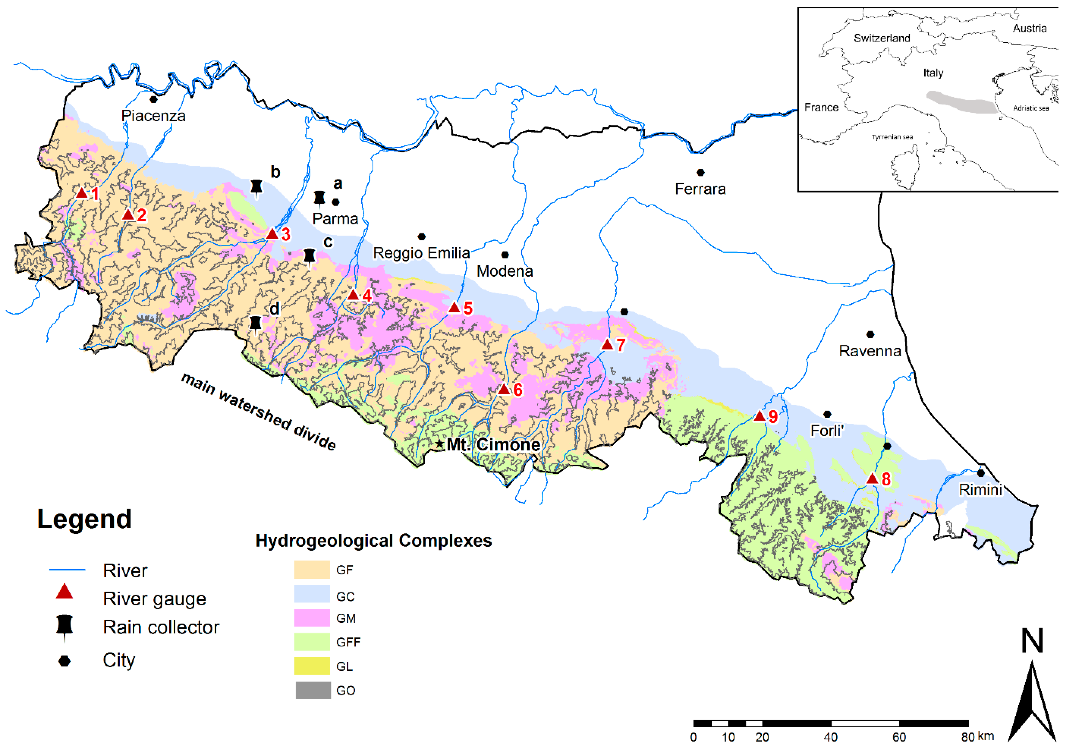
1. Introduction
Catchments are complex hydrological systems in which the understanding and quantification of the several processes participating in the final runoff is a challenge [
1]. This is because the hydrological processes are heterogeneous and their full understanding is not achieved even on small scales (i.e., that of the slope). Thus, extrapolating hydrological processes occurring at the slope scale to a larger scale (i.e., that of catchment) is difficult. Among others, oxygen (
18O and
16O) and hydrogen isotopes (
2H and
1H) compose the water molecules and have commonly been considered powerful tools for gaining information on the hydrological processes for a long time [
2,
3]. At the catchment scale, they have been extensively used to understand the runoff mechanisms by collecting isotopic data from the different components participating in the hydrological cycle. The number of components to be monitored depends on the type of catchment. For example, in glacierized catchments, the isotopic data of the snow and glacier melt water, in addition to those of precipitation and runoff, are essential [
4,
5]. In catchments located at lower altitudes, it is common to collect water isotopes from precipitation, runoff, soil moisture and groundwater [
6,
7,
8].
The above-mentioned studies have mainly involved small-catchments (in which areas are generally less than 100 km2) as the complexity and heterogeneity of hydrological processes are often less there. In larger catchments, the use of water isotopes may be less effective as the number of components with different isotopic compositions generally become higher and their signal unclear. For example, the runoff in large catchments can be fed by aquifers with different isotopic signals while rainfall may not have a unique isotopic value if it takes place at different altitudes (i.e., altitude effect).
Moreover, when considering the annual seasonality of isotope data, isotopic variations in river discharges are generally damped due to the times spent by water molecules travelling along the catchments (i.e., transit times) and to the contribution of groundwater, which has a relatively constant isotopic signal. As a result, the longer the paths are (and/or the larger is the contribution of groundwater to rivers) the more the variation of the isotopes in rivers is damped. In the case of large catchments characterized by long transit times or catchments in which the quota of groundwater in discharge is prevalent, the isotopic variation of isotopes in river water may even be nil [
9].
In addition, several processes can take place on a catchment scale modifying the former isotopic signal of precipitation collected in rain gauges. These processes are usually enhanced in large catchments. Among others and without claiming to be exhaustive, evapotranspiration occurring within the soils during specific periods of the year or anthropogenic impacts due to reservoirs, irrigation and water treatment plants are responsible for river water that is typically enriched in heavy isotopes compared to the precipitation. The same effect (i.e., river water enriched in heavy isotopes compared to precipitation) is related to sublimation processes acting on the snowpack accumulating in the uppermost parts of the catchments [
10,
11].
Due to the problems outlined above, few studies in the literature have used water isotope time-series to depict hydrological processes from large catchments worldwide (see, for instance and without claiming to be exhaustive: [
12,
13,
14,
15,
16,
17,
18,
19]). Consequently, even fewer studies have compared the temporal and spatial behaviour of water isotopes from rivers at a regional scale. A recent paper by [
20] has analysed the temporal and spatial patterns of water isotopes in nine large catchments from Germany and their relationships with isotopic composition in precipitation and some selected catchment characteristics. Firstly, the Authors confirmed that the use of the time series of water isotopes provides information on the hydrological processes in large catchments. Secondly, water isotopes in the river can deviate from the isotopic compositions of precipitations collected in the large catchments because of natural and anthropogenic processes such as evapotranspiration from the soils and river network as well as evaporation from reservoirs. Furthermore, they verified statistical associations between the average isotopic values recorded in catchments and some specific physiographic characteristics.
In this study, we have combined several existing datasets concerning both rains and rivers from the northern Italian Apennines, an area in which the runoff response to precipitation events is usually rapid in all the rivers due to the widely outcrop of clay-rich bedrocks. A final dataset was created and includes monthly isotopic data collected in 4 rain gauges (period January 2003–December 2006) and 9 rivers (period January 2006–December 2007). The data are integrated with the corresponding monthly discharges in river gauges where water isotopes were collected.
The purpose of this work is to verify which information can be gained by this short-time (2 years) isotopic dataset consisting of grabbed water samples from large catchments made up of clay-rich bedrocks. Despite the use of short-time (<3 years) and scattered isotopic series in rivers being uncommon, their temporal fluctuations should be enhanced by the poorly permeable bedrocks so that some hydrological information can be preserved. In this the paper, we will provide an overview of the spatial and temporal variability of isotopic composition in precipitations and river waters together with estimates of residence times in catchments. Finally, time series analysis of the isotopes in rivers is tested and possible statistical associations with selected catchment characteristics will be investigated.
5. Results
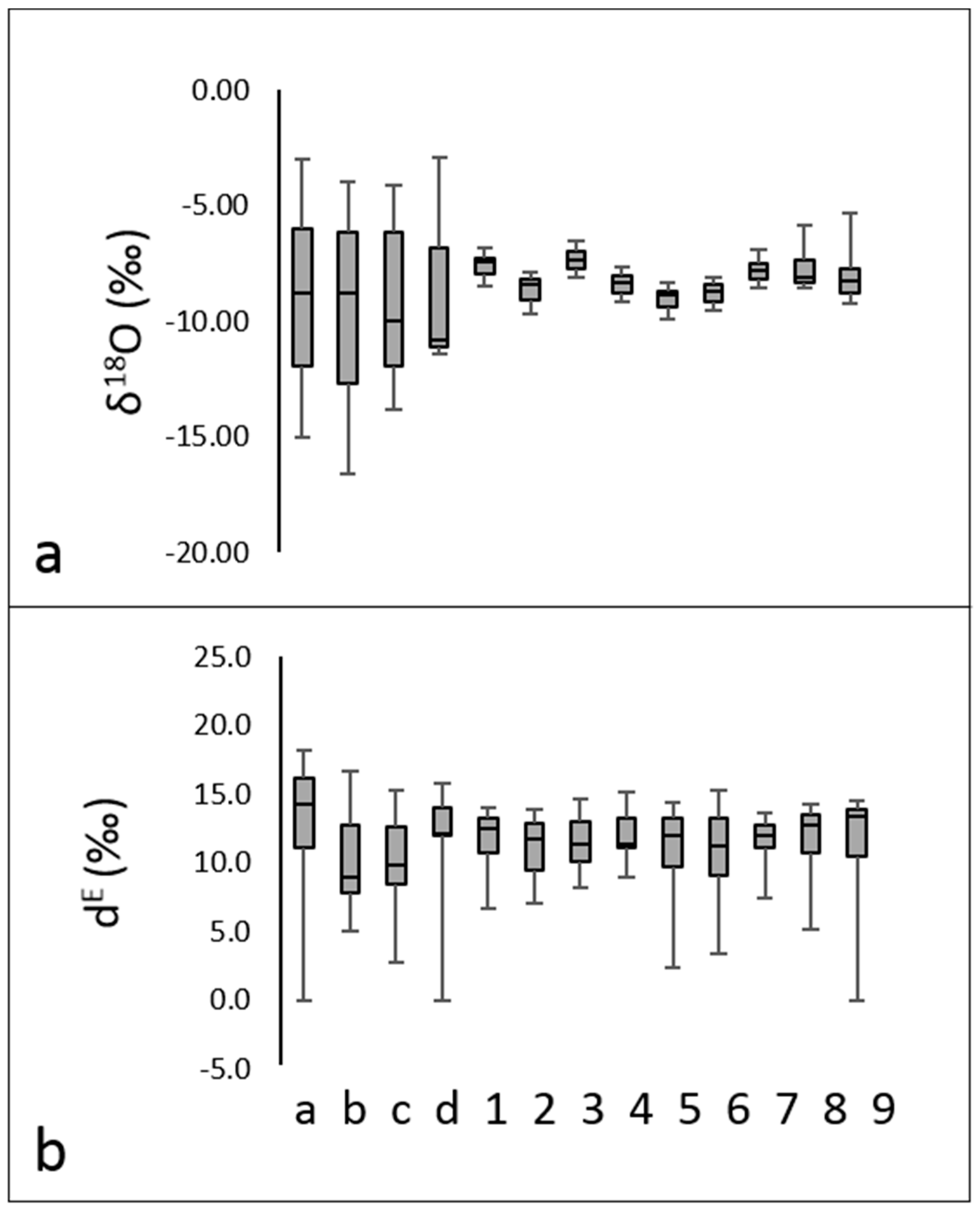
Table 3 summarizes the mean (
MA) and weighted (
Mw) values of δ
18O, δ
2H and d
E in water from the rain collector. δ
18O-
MA and δ
2H-
MA ranges from −8.96‰ (Parma) to −9.67‰ (Langhirano) and from −61.1‰ (Parma) to −67.5‰ (Langhirano). d
E is between 9.8‰ (Langhirano) and 10.6‰ (Parma). Distributions of δ
18O and d
E values from rain collectors were skewed, with mean values that may differ remarkably from the median (see box plots in
Figure 2). Weighted averages (δ
18O-
MW and δ
2H-
MW) were slightly negative than the aforementioned unweighted means being between −9.48‰ (Parma) and −9.93‰ (Langhirano) and −64.3‰ (Parma) and −69.1‰ (Langhirano), respectively. In all the rain collectors, d
E-
MW was higher than the corresponding
MA values as they ranged from 10.3‰ (Langhirano, Berceto) to 11.6‰ (Parma). The aforementioned variation between
MA and
MW pair values is due to the fact that precipitation amount as well as its isotopic composition is not uniformly distributed during the year. In detail, and with reference to the Parma rain collector (here considered as representative of the behaviour of others rain collectors, as clearly visible in
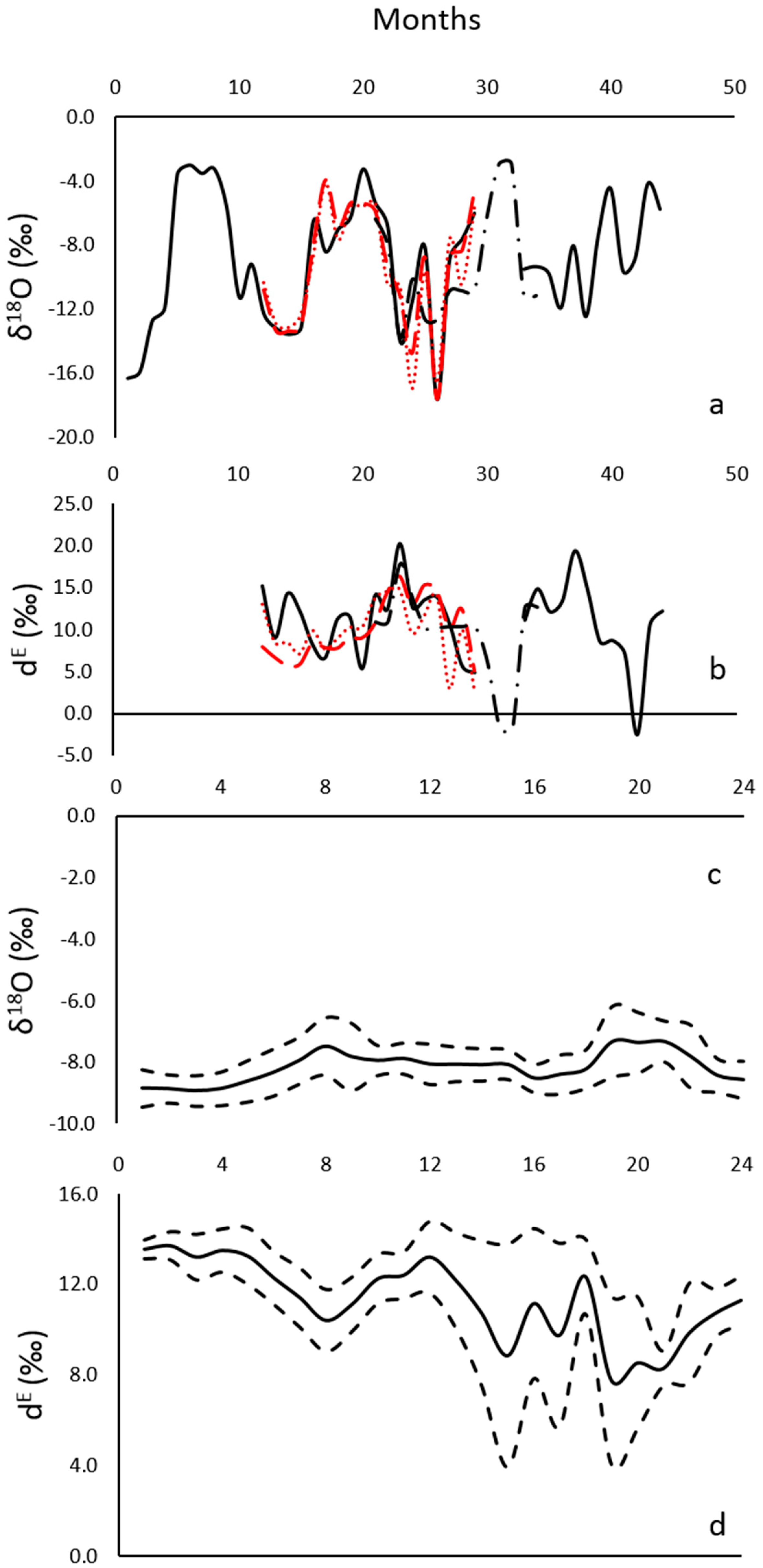
Figure 2a), δ
18O values showed seasonal variations with a minimum in winter (February 2005: −17.64‰) and a maximum in summer (July 2003: −3.02‰).
The same behaviour is noticed for δ
2H (not shown in
Figure 2 being characterized by the same pattern of the δ
18O), which in case of the Parma rain collector showed a minimum of −127.3‰ (February 2005) and maximum of −13.41‰ (July 2003). When δ
18O-
MW and δ
2H-
MW were more negative than the corresponding δ
18O-
MA and δ
2H-
MA, this meant the specific year was characterized by a larger amount of winter precipitation (i.e., more depleted isotopic values) and/or a lower quantity of summer precipitations. As d
E is obtained from the data of δ
18O and δ
2H, its composition in precipitation varies during the year and is usually higher in the period between the end of the autumn and spring seasons (
Figure 2b; November 2004: 20.2‰; January2006: 19.3‰) and lower in summer (June 2006: −2.3‰). As a result, a larger amount of autumn-spring precipitations leads to a higher value of d
E.
By considering the river waters (
Table 4 and
Figure 2c,d), unweighted means are more positive than the corresponding values from rains. In fact, the δ
18O-
MA are included between –7.46‰ (Taro) and −9.01‰ (Secchia) while δ
2H-
MA are between −48.2‰ (Taro) and −61.4‰ (Secchia), respectively. d
E-
MW values are slightly higher than in the rain as they range between 10.5‰ (Secchia, Panaro) and 12.0‰ (Enza). By considering the weighted averages, all δ
18O-
MW values became more negative as they are between −7–60‰(Taro) and −9.09‰(Secchia).
δ2H-
MW values were not all more negative than
δ2H-
MW and are included between −48.5‰ (Trebbia) and −61.1‰(Secchia). The d
E-
MW values are slightly more positive than the corresponding d
E-
MA being between −10.4‰ (Panaro) and 12.7‰ (Secchia). As in the case of precipitation, the mismatch between unweighted (
MA) and weighted averages (
MW) pair values reflects an isotopic composition that was not uniformly distributed during the year (
Figure 2c). In fact, water in rivers was much more enriched in
δ18O at the end of the summer season (June, July, August) when the flow rates were lower.
Samples from rivers showed a strong attenuation of the δ
18O signatures in comparison with precipitation data (
Figure 3). In detail, the Lamone and Savio rivers were characterized by a higher dispersion of the δ
18O values than the other rivers. On the contrary, d
E distributions from river samples were poorly attenuated with box limits (i.e., the 25th and 75th percentiles) that are often in range with those from rain water (
Figure 3). This was evident for the Secchia, Panaro, Savio and Lamone rivers.
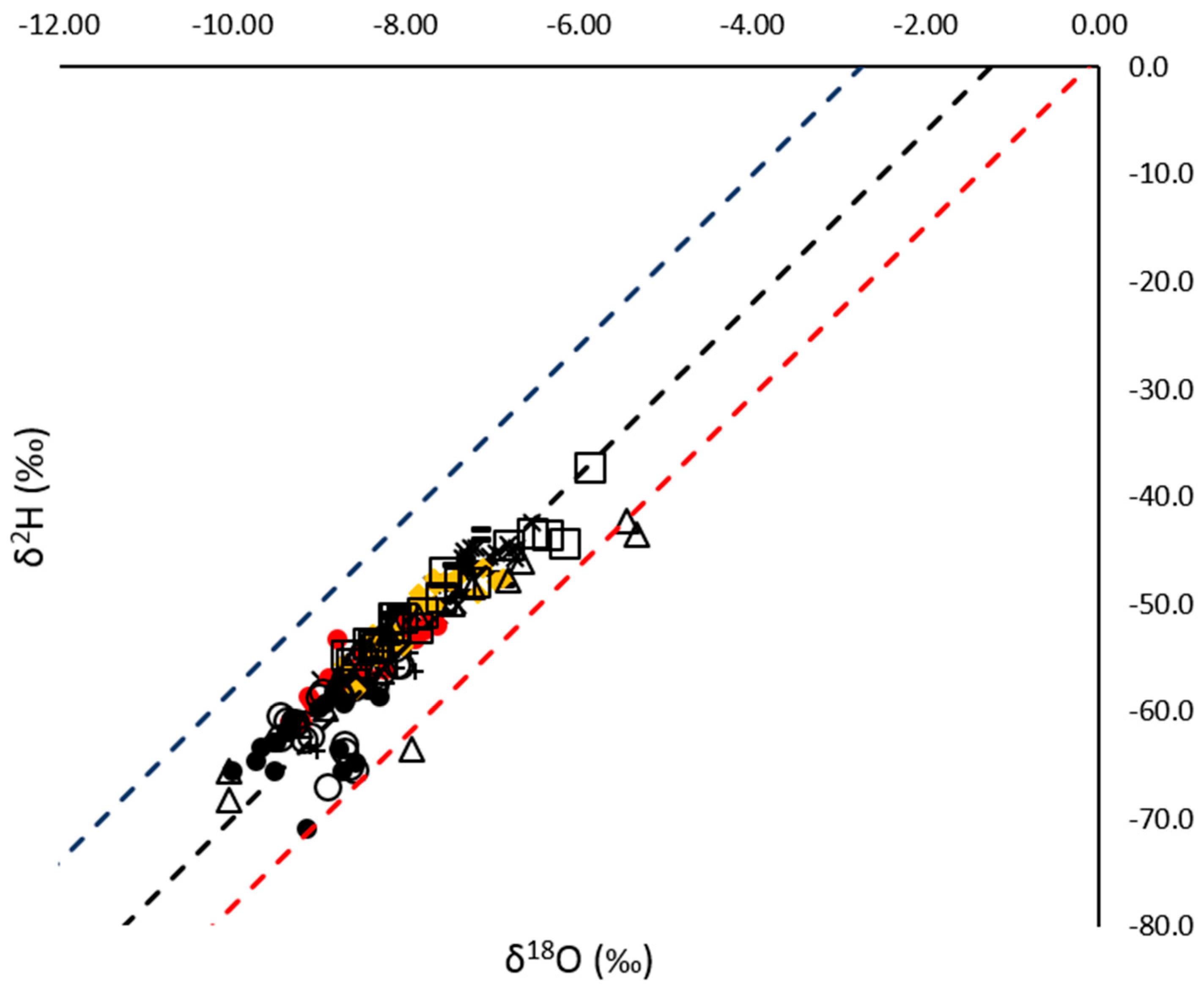
δ
18O and δ
2H were correlated, both in the case of precipitation and river water. The δ
18O–δ
2H relationships are summarized in
Table 3 (Meteoric Water Lines MWLs from rain gauges) and
Table 4 (River Water Lines RWLs from rivers), in which slopes, intercepts and coefficients of determinations (R
2) are reported separately. Slopes obtained interpolating δ
18O–δ
2H pairs from rain collectors (MWLs) ranged between 6.9 (Berceto) and 7.8 (Lodesana, Langhirano). With the exception of the Berceto rain collector (−1.9), all intercepts were positive, being between 6.9 (Parma) and 7.8 (Lodesana). Slopes from RWLs were lower and ranged from 4.3 (Secchia) to 6.2 (Taro). Intercepts were always negative showing values from −2.0 (Taro) and −22.8 (Secchia). In the case of the Secchia and Panaro rivers, R
2 values (0.33 and 0.36, respectively) indicate weaker correlations that are due to 4 monthly samples from January 2017 to April 2017 lying far below the alignment of the others (not shown).
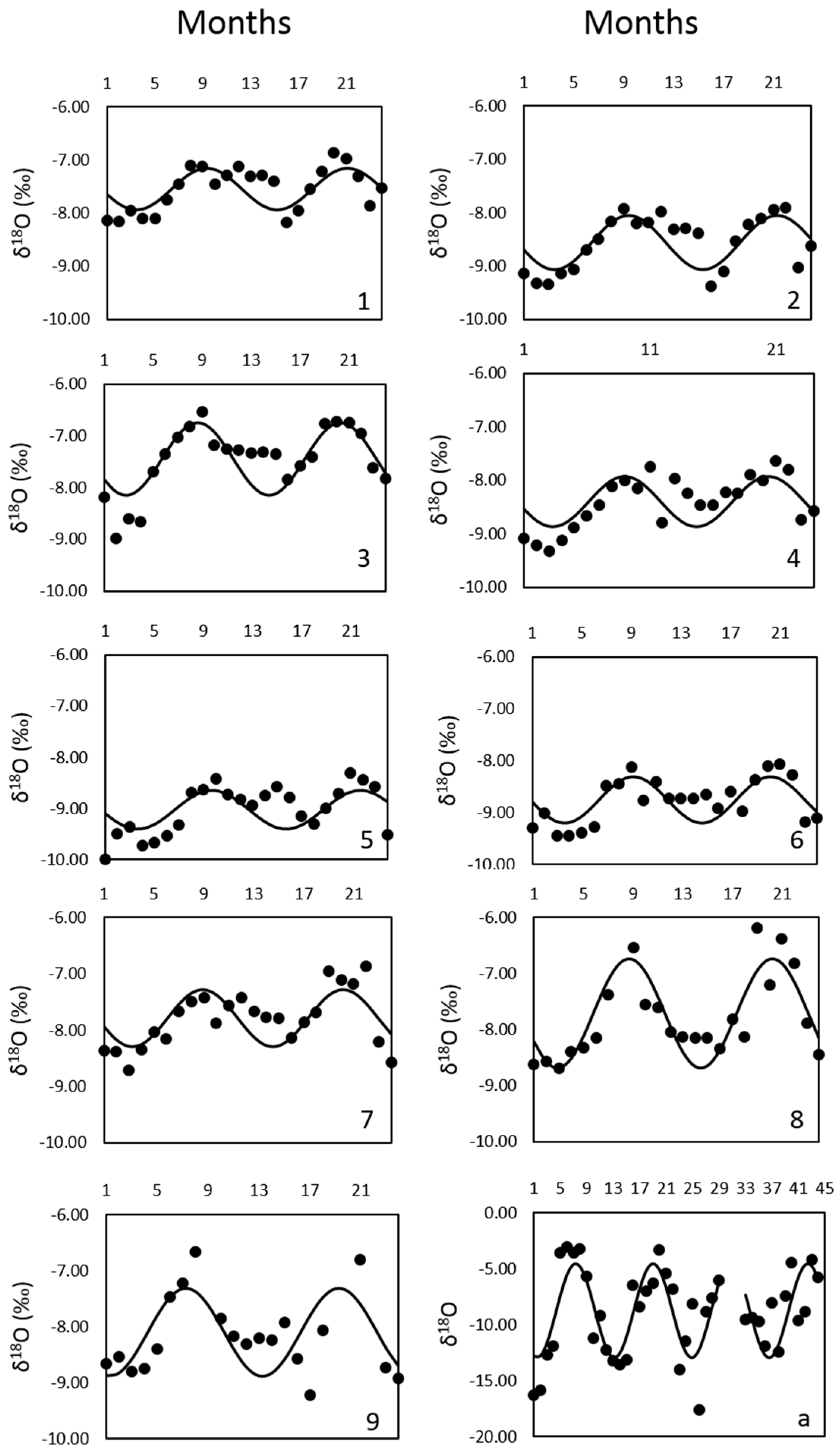
As described in
Section 4.2, residence times of the river were estimated starting from a representative input function (
Figure 4). A sinusoid was fitted to the δ
18O data of precipitation and the corresponding amplitude (
Ain = 4.250) together with the goodness of fits are summarised in
Table 5. Fit was statistically robust (
p < 0.0001) and the coefficient of determination was in the order of those obtained in other studies (see, for instance: [
52,
53,
54]).
Modelled output sinusoids for rivers are also reported in
Table 5. With the exception of the Savio River (
p value remarkably higher than 0.0001 and R
2 = 0.30), the fits were characterized by coefficients of determination (R
2) that were higher than 0.48 and always, or close to being, statistically significant (
p < 0.0001). Amplitudes of output sinusoids (
Aout) differed slightly as they were between 0.397 (Secchia) and 0.974 (Lamone).
MRTs were estimated with Equation (5) and are also reported in
Table 5; they ranged between 8 (Lamone) and 21 (Secchia, Trebbia) months. As shown in
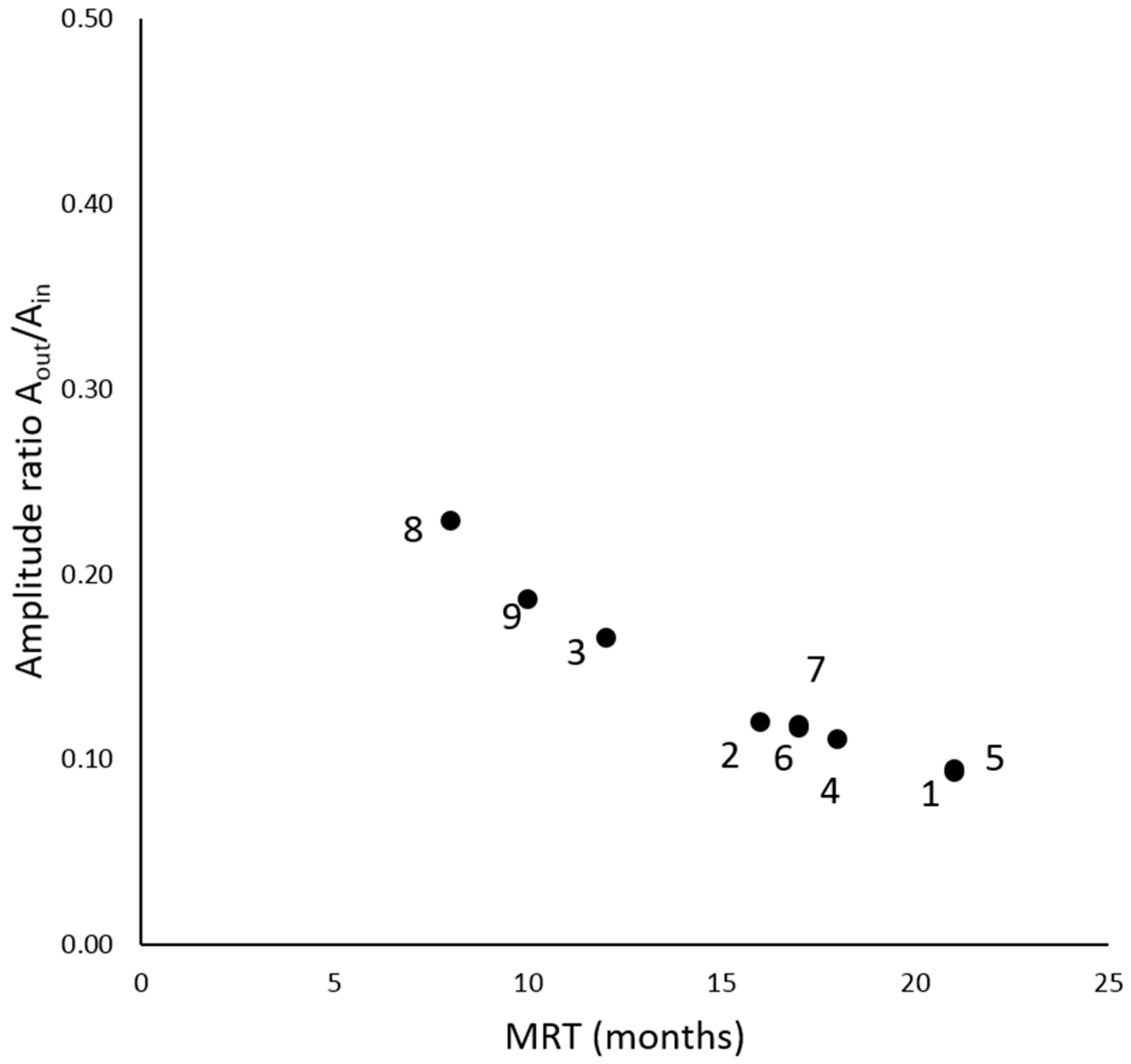
Figure 5, the relationship between the
Aout/
Ain ratios and the MRTs for the 9 catchments deviated little from a linear function, indicating a reduced effect of aggregation bias on the MRT estimates due to a large quota of river waters with fast transit time (lower than 1 year). Thus, the consequent underestimation effects did not significantly affect the final MRT values.
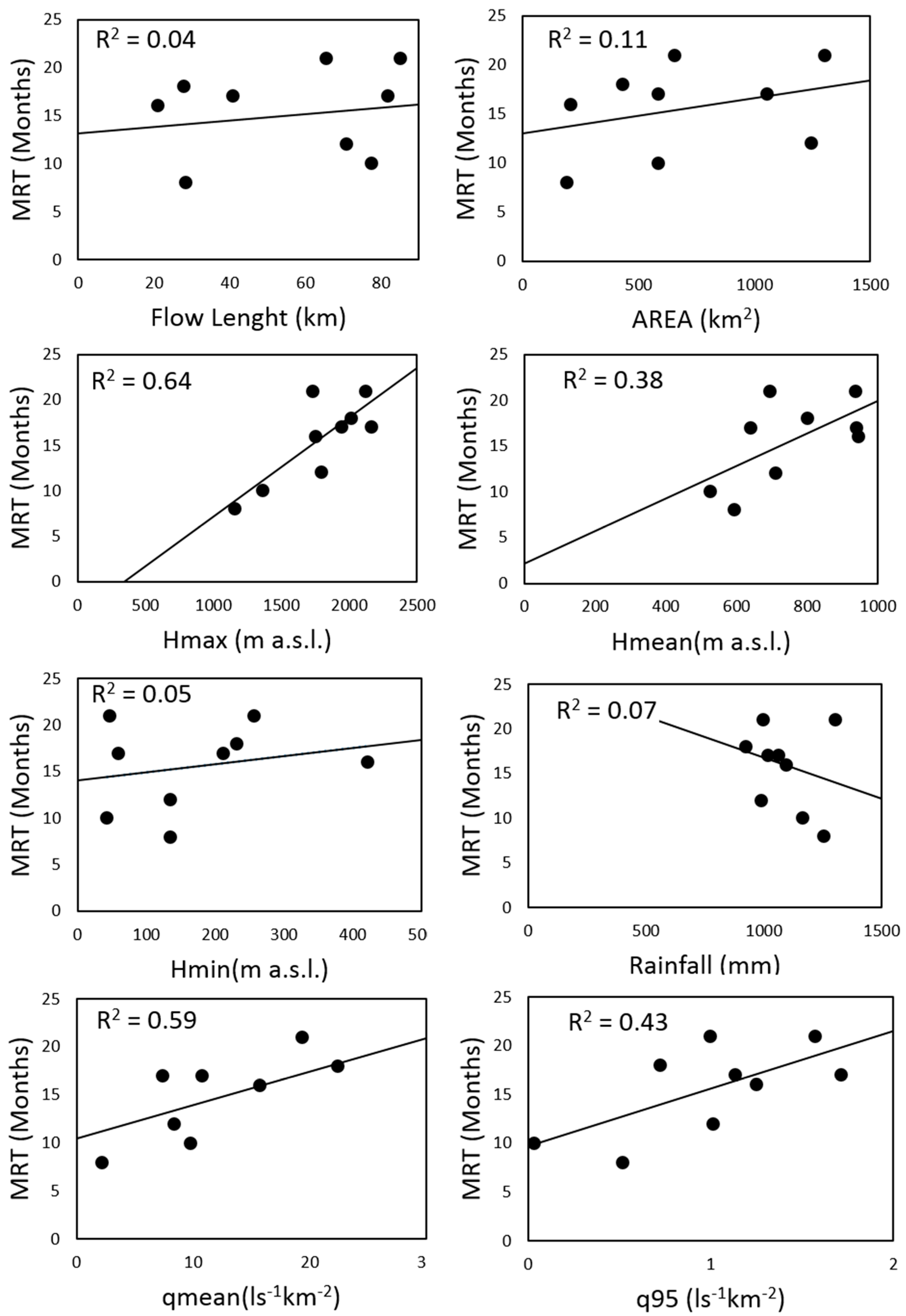
Linear relationships between catchment characteristics and the weighted δ
18O and d
E averages were not significant as
p values were always greater than 0.01 (plots are not reported). On the contrary, some catchment characteristics were correlated with the MRTs of rivers (
Figure 6). This was the case for the mean annual specific runoff (q; R
2 = 0.59 and
p < 0.01), the maximum altitude (Hmax; R
2 = 0.63 and
p < 0.01) and the specific low flow discharge q95 (R
2 = 0.44 and
p < 0.01).
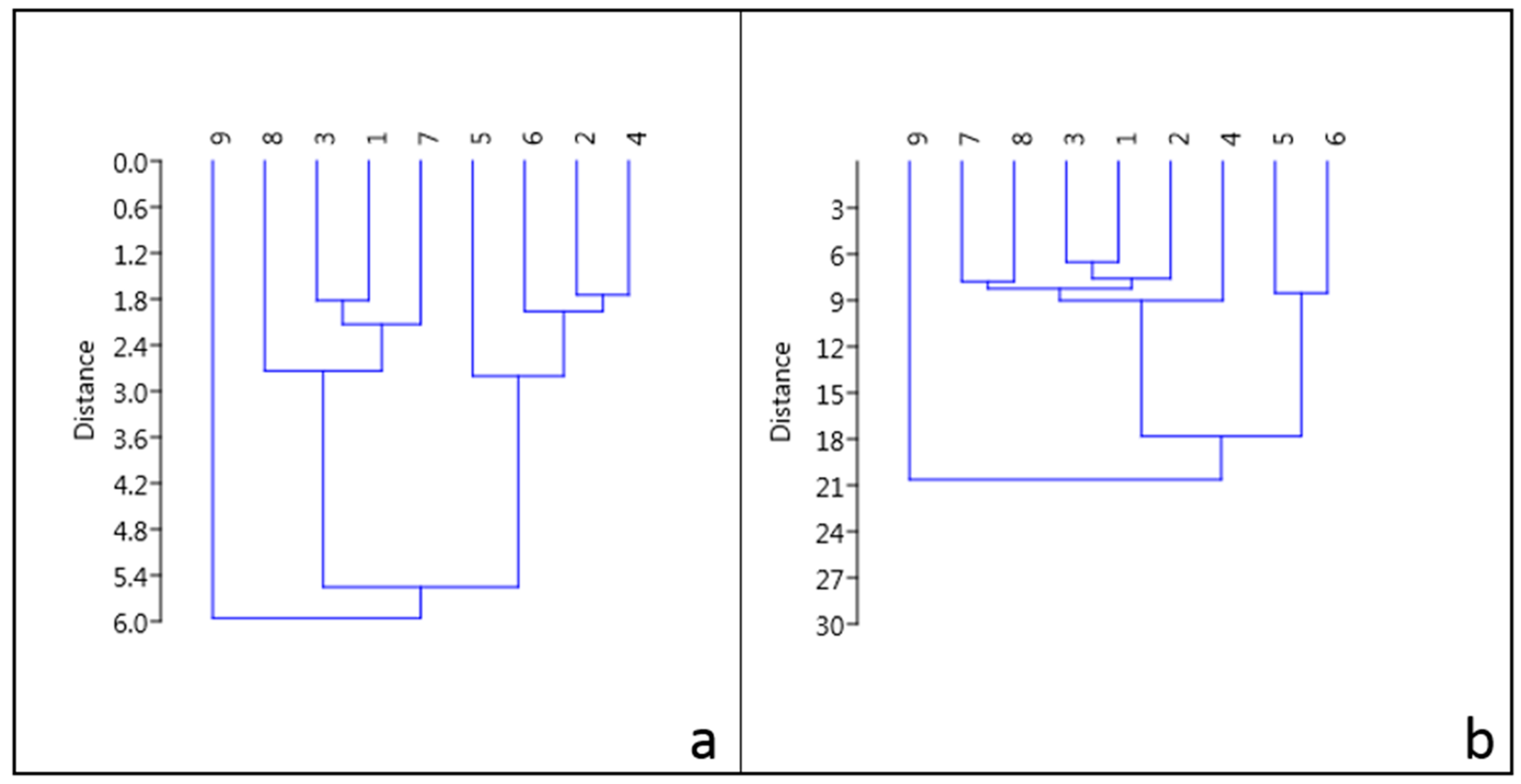
In
Table 6, correlation coefficients between pairs of δ
18O time series from the 9 rivers are reported in the form of a correlation matrix (Manova analysis). With the exception of the south-easternmost river of the area (Savio River), the monthly isotopic composition of rivers strongly correlated with each other (R
2 > 0.67). However, some pairs of rivers were characterized by higher correlation coefficients: this is the case of Trebbia-Nure and Secchia-Panaro rivers, with R
2 equal to 0.95 and 0.93, respectively. The cluster analysis (
Figure 7a) among the δ
18O time series from rivers demonstrated that the Savio river was associated with none of the other rivers while two main groups of catchments were clearly separated: the first one comprises Enza, Nure, Secchia and Panaro while the other group was Trebbia, Taro, Reno and Lamone. Different results were obtained from the analyses of the d
E time series: correlation coefficients were always lower than in case of δ
18O time series and more rivers were not associated with each other (see
Table 7 and
Figure 7b). In detail, the d
E time series of Taro, Trebbia and Nure were associated, as well as those of Secchia and Panaro. This was also the case of the d
E time series from Lamone and Reno rivers.
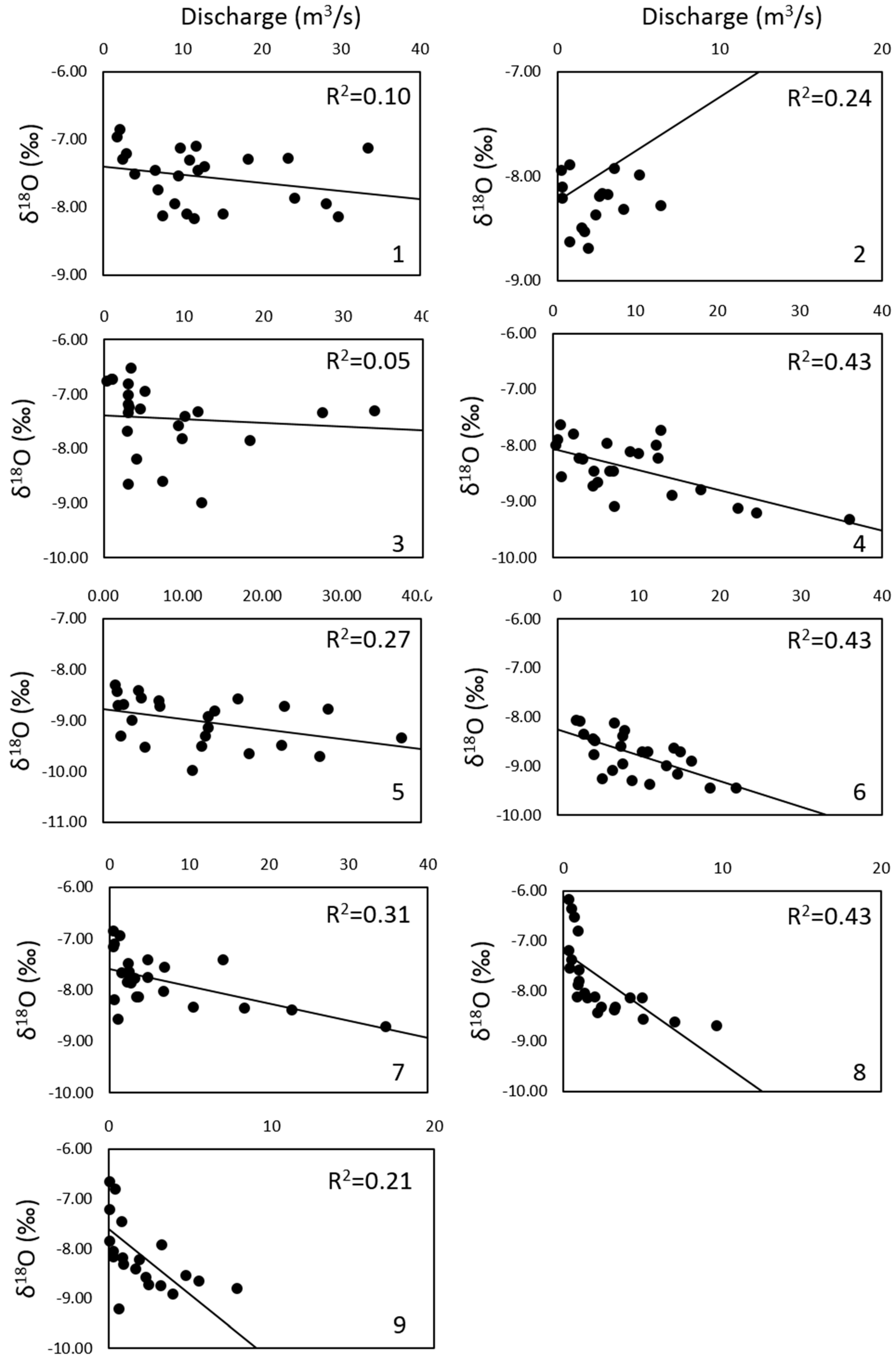
River monthly discharges affected the isotopic composition of river water. In detail, with the exception of the Taro river, values of δ
18O depleted with increasing flow rates (
Figure 8). On the contrary, the d
E values in the river water increased with discharge in almost all rivers (
Figure 9). In the case of δ
18O-discharge relationships, statistical analyses were significant for 4 rivers (Enza, Panaro, Reno, Lamone). In some cases (namely: Lamone and Savio), the relationship looks exponential rather than linear. d
E -discharge linear regressions were statistically significant for 5 rivers (Trebbia, Nure, Enza, Lamone). It must be specified that, as in the case of δ
18O-discharge relationships, d
E-discharge regressions also appeared to be exponential (Reno, Lamone, Savio).


