Comparison and Analysis of Different Discrete Methods and Entropy-Based Methods in Rain Gauge Network Design


1
State Key Laboratory of Simulation and Regulation of Water Cycle in River Basin, China Institute of Water Resources and Hydropower Research, Beijing 100038, China
2
Department of Water Resources, China Institute of Water Resources and Hydropower Research, Beijing 100038, China
3
Sichuan Research Institute of Water Conservancy, Chengdu 610072, China
4
School of Hydraulic Engineering, Dalian University of Technology, Dalian 116024, China
*
Author to whom correspondence should be addressed.
Water 2019, 11(7), 1357; https://doi.org/10.3390/w11071357
Submission received: 10 June 2019
/
Revised: 24 June 2019
/
Accepted: 27 June 2019
/
Published: 30 June 2019
(This article belongs to the Section Water Resources Management, Policy and Governance)
Abstract
:A reasonable rain gauge network layout can provide accurate regional rainfall data and effectively support the monitoring, development and utilization of water resources. Currently, an increasing number of network design methods based on entropy targets are being applied to network design. The discretization of data is a common method of obtaining the probability in calculations of information entropy. To study the application of different discretization methods and different entropy-based methods in the design of rain gauge networks, this paper compares and analyzes 9 design results for rainy season rain gauge networks using three commonly used discretization methods (A1, SC and ST) and three entropy-based network design algorithms (MIMR, HT and HC) from three perspectives: the joint entropy, spatiality, and accuracy of the network, as evaluation indices. The results show that the variation in network information calculated by the A1 and ST methods for rainy season rain gauge data is too large or too small compared to that calculated by the SC method, and also that the MIMR method performs better in terms of spatiality and accuracy than the HC and HT methods. The comparative analysis results provide a reference for the selection of discrete methods and entropy-based objectives in rain gauge network design, and provides a way to explore a more suitable rain gauge network layout scheme.
1. Introduction
Rainfall data are important basic data in hydrological and water resources research. These types of data are some of the main driving data forms in water resource evaluation, water cycle simulation [1,2,3,4], and water use efficiency calculation [5,6]. How to construct a scientific and reasonable rainfall network to obtain rainfall data has always been the most basic and important part of hydrological measurement work. With the development of the entropy theory in hydrological analysis [7,8,9], many types of information entropy have been developed that can reflect the degree of information correlation between stations. This information entropy has been gradually applied to the design of rain gauge networks with the advantages of efficient calculation, clear theory and high practicability [10,11,12,13]. However, the process of calculating probability density from rainfall data as continuous data is complex when calculating information entropy. Furthermore, reasonable discrete rainfall data that can be used to obtain the corresponding probability are still a problem in the application of the information entropy method to the design of rainfall networks, and a variety of network design methods that describe the information content do not have relevant comparisons. Comparing and analyzing the results of different discretization methods and the influences of different entropy-based optimization objectives in rain gauge network design involves the use of some realistic meanings and research values, which can also provide a reference for better application of information entropy theory and rainfall network design.
Data discretization methods can be classified into three categories: equidistant discretization, equiprobable discretization and adaptive discretization [14]. Equidistant discretization divides all data into bins of the same width, and the probability of each value is estimated by the frequency of the numerical sample, such as the rounding method. Equidistant discretization divides the data for each variable into bins of the same total number, in which the bin width of each variable is not necessarily the same. For hydrological data, this method is seldom used. Adaptive discretization is used to calculate the width of the bin according to the sequence characteristics of the variables, i.e., the number and width of the bins of each variable are different. The size of the bin is calculated according to the length, range of extreme values, mean and variance in the sequence of variables; this is the most widely used method [15,16,17,18,19,20]. Many scholars have compared and analyzed the influence of various discretization methods on the entropy value. Singh [21] concluded that the entropy value decreases with increases in the bin width and/or time interval by using seven time series of interval runoff data to perform discretization at different equidistances. Both the bin width and time interval have a significant influence on the entropy value. Papana et al. [14] compared and analyzed the differences in the mutual information estimators of equidistant discretization, adaptive discretization, k-nearest neighbor and the kernel method in estimating mutual information values based on a Monte Carlo simulation of time series data with different noises. The results show that the bin method is effective and stable in the presence of noise. Alfonso et al. [22] and Li et al. [23] considered that the equidistant discretization of measured data can filter out some small data fluctuations. Dispersion that is too dense causes the amount of information between sites to be similar, makes it difficult to distinguish the information content retained by each site, and leads to inconveniences in further analysis, while dispersion that is too sparse will miss some information values. Fahle et al. [24] used groundwater level data to compare the differences between two typical equal spacing and adaptive discretization methods. He considered that the rounding method can effectively eliminate noise, while the SC method proposed by Scott [17] may not reflect the sudden change in data due to variance change. Keum [25] considered that with the increase in the number of stations, the influence of discrete methods on the results decreases, and while the discrete methods affect the ranking of stations, the calculation of mutual information and the layout of stations, the rounding, the SC method and the ST method proposed by Sturges [20] can all be effectively discretized. Wang et al. [26] considered that the information entropy calculated by the rounding method and three adaptive discretization methods is consistent with the characteristics of regional precipitation when using information entropy and time variability analysis to optimize a rainfall network. Because of the maximum entropy value calculated, the SC method was used in practical applications in her study.
Many scholars have proposed different network optimization objectives in the application of entropy theory in the design of a network. Yoo et al. [27] refers to optimizing the layout of a rainfall station network with the maximization of internal information and mutual information from other stations. Alfonso et al. [28] optimized the layout of water level monitoring stations according to the maximization of internal information and the minimization of redundant information. Alfonso et al. [22,29] suggested that the maximization of internal information and the minimization of mutual information in the network are designated as optimization objectives to design a water level and runoff monitoring network. Using the same optimization objective, James Leach et al. [30] and Samuel et al. [31] determined a network design for monitoring groundwater runoff, and other station data were combined with physical hydrologic characteristics and regionalization methods. Chen et al. [32], Yeh et al. [33,34], Wei et al. [35], Su et al. [36], and E. Ridolfi et al. [37] removed the points with maximum conditional entropy to join the network to ensure that the effective information of the network was maximized, and the network that satisfied a certain proportion of the information was designated as the optimal layout result. Li et al. [23] proposed a maximum information and minimum redundancy method (MIMR) for station network design, where the maximum joint entropy, minimum redundancy and maximum mutual information of unselected stations are designated as optimization objectives, and the greedy selection algorithm is applied to solve the optimal rainfall network. This method has been widely used in the design of rainfall networks [25,26,38,39].
It is undeniable that different discrete methods and different optimization objectives have certain effects on the layout results of a rain gauge network, but there is still a lack of specific quantitative comparison and analysis of discrete methods and entropy objectives. The purpose of this paper is to compare and analyze the application effects of commonly used discrete methods and methods of rainfall network design based on information entropy to provide a reference for the improved application of information entropy theory to the optimal layout of a precipitation monitoring network. The article is divided into five sections. The second section mainly introduces the research methods, including the discrete method and information entropy calculation, and the optimization of the network design methods; the third section mainly introduces the research area and data situation; the fourth section discusses the comparison of different methods and different objectives; and the fifth section discusses the conclusion and outlook.
2. Methodology
The design of a rain gauge networks based on entropy is mainly divided into the following steps: (1) the discretization of data to obtain the probability associated with different values; (2) the calculation of a variety of information entropy types based on the probability, such as the marginal entropy, joint entropy, mutual information entropy, etc.; (3) obtaining the optimal network design results according to the combined information entropy among different networks; and (4) updating the existing network until it meets the relevant requirements; then, new precipitation data are obtained by using kriging interpolation.
2.1. Data Discretization
Among the many data discretization methods [40], equidistant discretization and adaptive discretization are the most widely used in the calculation and analysis of hydrological station networks. In this paper, three of the most common discretization methods are selected for comparative analysis. The first is the rounding method [22], which is expressed as:
where denotes the discrete value of the data sequence, denotes the original value, denotes the adjustment factor, and denotes the integral function. This method is a rounding method with distance , which varies according to the variables. For example, the value of the runoff data is 150 [23], and the values of the rainfall, water level and discharge data are usually 1 or 5 [22,25]. In this paper, the value of is 1, which is denoted as the A1 method. The second method calculates the optimal bin value proposed by Scott [17]. The expression is as follows:
where is the standard deviation of a data sequence observation series and is the total number of data series; this method is abbreviated as the SC method in this paper. The third method calculates the optimal bin value proposed by Sturges [20]. The expression is as follows:
where is the range of the data sequence observation series and is the total number of data series; this method is abbreviated as the ST method in this paper.
2.2. Entropy
In 1948, Shannon obtained the uncertainty degree of random variables based on probability calculation and then put forward the theory of information entropy [41]. The uncertainty of the variables or the amount of information expressed becomes greater as the entropy value becomes greater. Assume that the values of the discrete random variables X and Y are and , respectively. and denote the probability of occurrence of event X and the joint probability of X and Y, respectively. Several conceptual expressions of entropy are as follows. The expression for calculating the marginal entropy is as follows:
The marginal entropy represents the comprehensive information quantity of two variables, and its calculation expression is as follows:
Transinformation represents the amount of mutual or redundant information between two variables. The expression is as follows:
Conditional entropy represents the amount of information when a variable is independent of another variable. The expression is as follows:
The information transfer index (ITI) represents the information transfer between two variables and more intuitively expresses their redundancy and correlation. The computational expression is as follows:
Notably, , where the information flux becomes greater and the degree of correlation is higher as the ITI value in the [0, 1] interval becomes greater [42]. In the design of a raingauge network, X represents a rain gauge, and represents its precipitation sequence. The expression of the joint entropy of a network composed of N rain gauges is as follows:
The expression of the redundant information of a network composed of N rain gauges, C, is as follows:
2.3. Optimization of Network Design
There are many hydrological station network design methods based on information entropy theory. This paper mainly compares and analyses three widely used optimization objectives.
First, the comprehensive information quantity of the network is evaluated by the maximum newest point and the condition entropy method of the network; that is, the mutual information dataset of the station network is the smallest [32], and the screening expression is as follows:
where denotes the number of existing sites in the network and is one of the N potential sites ; the same definitions apply below. This method is abbreviated as the HC method in this paper.
Second, the maximum internal joint entropy and the minimum mutual information method are used to ensure the maximum comprehensive information of the network [22] (abbreviated as the HT method). The expressions are as follows:
Third, the maximum joint entropy, the minimum redundancy of the network and the maximum mutual information are designated with the unselected points as the three conditions to ensure the optimal comprehensive information of the network [23]. The expression is as follows:
A greedy ranking algorithm [23] is an effective simplified sorting method that converts a multiobjective problem into a single-objective problem. By transforming the addition and subtraction of multiple elements into a comprehensive parameter, most sites are then selected according to the comprehensive parameters.
Then, the final expression of the above three optimization objectives is as follows:
2.4. Kriging Interpolation
The kriging method is a spatial interpolation method proposed by D. G. Krige, a South African mining engineer [43]. The main principle of this method is to apply the variation distribution of the modulus of the sample points, assign different weights to each sample point according to the spatial position distance and correlation degree, and then obtain the estimated value of the interpolated point by taking a sliding weighted average. Moreover, this method satisfies the two conditions of minimum difference between the estimated value and the true value and unbiased estimation. The expressions are as follows:
where is the estimated value at and is the weight coefficient. There are many types of kriging interpolation methods according to different assumptions. The assumption of ordinary kriging interpolation is that every point in space has the same expectation and variance, that is, the spatial attributes are homogeneous, and the value at any point is equal to the sum of the mean value and the random deviation at that point. The spatial characteristics of the sampling points can be obtained by calculating the semivariogram values of the regionalized variables at different distances . The expression is as follows:
The empirical model is typically used to fit the semivariance function. The commonly used fitting models are the circle model, spherical model, exponential model, Gauss model and linear model. The spherical model is often used to fit rainfall data.
3. Study Area and Data
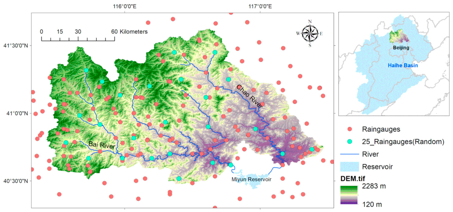
The research area in this paper is the upper reaches of the Chaobai River tributaries in the Haihe River Basin in China. The Chaobai River originates from the North China Plain, with a semihumid and semiarid continental monsoon climate. The two tributaries, the Chao River and Bai River, are joined at the Miyun Reservoir, which is one of the water supply reservoirs in Beijing, from the northwest and southeast, respectively. The study area is shown in Figure 1. The area of the study region is 136,000 km2. According to statistics, the average temperature is 9–10 °C, the topography is higher in the northwest and lower in the southeast, and the overall elevation is east-west trending, with an average elevation of 1010 m. The average annual precipitation is 300–400 mm, and the precipitation from June to October accounts for more than 85% of the total annual precipitation. There are 200 rain gauges in the study area and its surrounding areas, which can provide daily precipitation data.
Due to the lack of actual rainfall data in 2014, this paper uses the daily observed data from June to October in 2006–2016 (excluding 2014) for a total of 10 years (1530 days). In the experiment, 25 rain gauges were randomly selected as an assumed exiting network of the study area, and the interpolation data of all rain gauges around the study area were designated as the true values to verify and evaluate the final results. In addition to the measured data of the existing network, the Precipitation Estimation from Remotely Sensed Information Using Artificial Neural Networks-Cloud Classification System (PERSIANN-CCS), a remote sensing satellite precipitation product with high spatial and temporal resolutions, was selected to assist in evaluating the spatial layout of the network. Details of remote sensing data and their applications can be found in documents [44,45,46,47].
To ensure the accuracy of remote sensing data, the remote sensing data were screened and compared with the true value data. After screening, the remote sensing products with correlation coefficients greater than 0.5 were screened again for subsequent experiments, where the original 1530 days were reduced to 1196 days. The spatial correlation coefficient in the study area essentially remained above 0.6. In this paper, a resolution of 4 km × 4 km/pixel for the remote sensing spatial scale is used. The total number of pixels in the study area is 909.
4. Results and Discussion
4.1. Computation and Distribution of Entropy
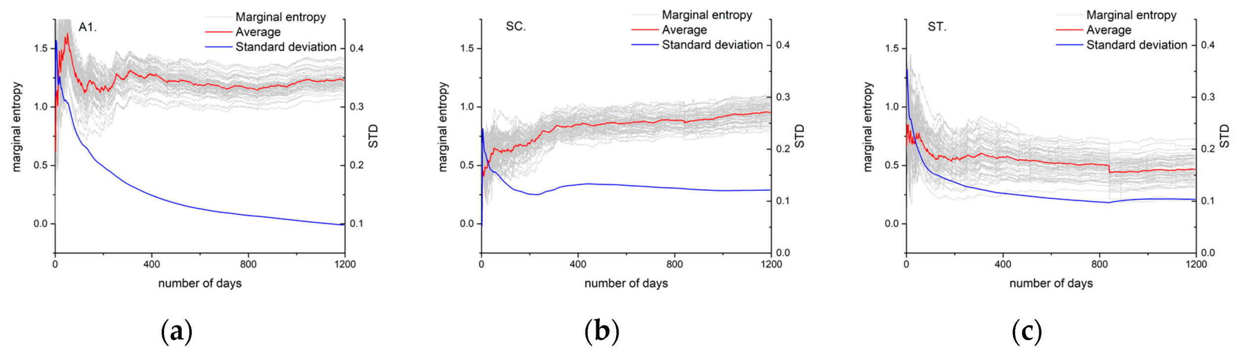
The literature [48] concludes that stable information entropy can only be calculated from data series of at least 10 years based on network layout experiments using data with different time series lengths. The 10-year rainy season rainfall data series selected in this paper were screened for a total of 1196 days. The marginal entropy for a single site is in the range of [0, log2 (1196)], i.e., [0, 10.58 bites]. Figure 2 shows the variation in marginal entropy of the measured rain gauges with the increase in time series length. The trend of the marginal entropy by the three discretization methods is basically the same, which increases first and then gradually becomes stable. When the time series is less than 300 days, the three types of marginal entropy experience unsteady fluctuations, and the variance is relatively high, which shows that only one or two years of data is not enough to capture more objective information. When the time series is longer than approximately 500 days, the standard deviation of various marginal entropy is approximately 0.1, and the amount of information at each point tends to have a stable value, that is, the information value of that point. To some extent, this also shows that the amount of information may be relatively small due to frequent precipitation during the rainy season. Furthermore, the application data of the rainy season for the design of rain gauge networks can even be applied to time series data that are slightly shorter than 10 years.
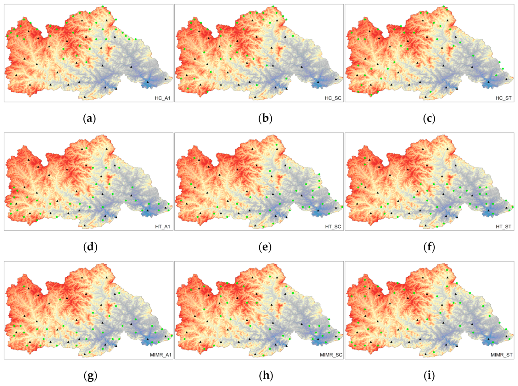
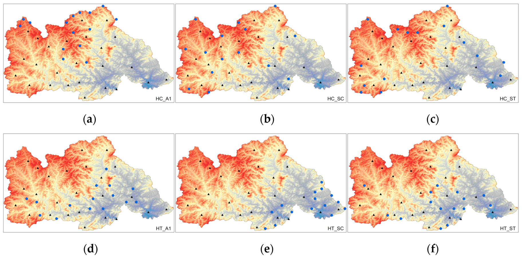
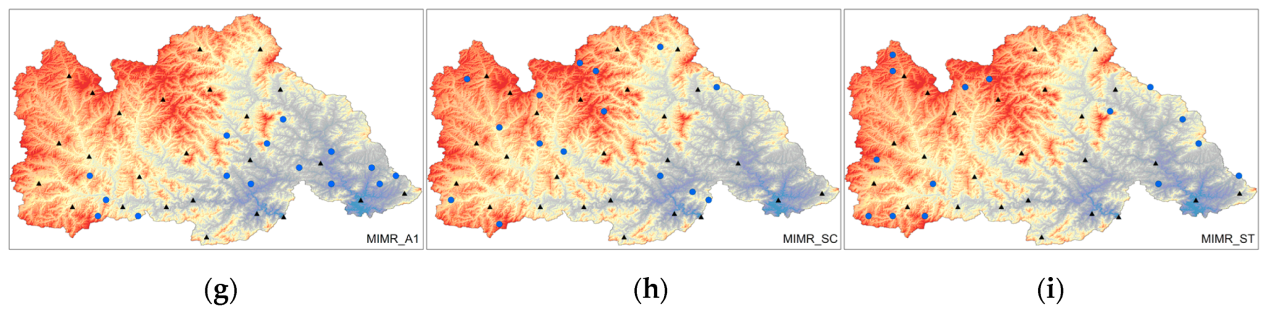
The three entropy-based methods discussed in Section 2.4 are applied to optimize the layout of rain gauges in the study area. The results are shown in Figure 3 and Figure 4. In an intuitive network layout, different discretization methods and optimized entropy indexes lead to significant differences in network design. Among the 60-raingauge network layout results, the results of the same layout method using different discretization methods are closer, while the results of the 40-raingauge network are more dissimilar after using different discretization methods. Generally, the results have obvious clustering characteristics when using the A1 discretization method, which may be due to the excessive retention of data change information. Compared with the A1 discrete method, the results of the SC and ST discrete methods are more in line with the terrain characteristics. Both methods show that there are more rain gauges in mountainous areas and fewer rain gauges in plain areas. Among the three layout methods, the HT layout method is less affected by the discrete method, and the results of site layout using different discrete methods are similar. The results of the HC and MIMR layout methods are relatively scattered and intuitively more reasonable.
4.2. Comparison of Information
The information content of a network has always been one of the main goals or objectives of many network design methods. Different discretization methods inevitably result in different information entropy values. The variation range of the entropy values of a raingauge network and a single point are considered, as shown in Table 1, and the results of the proportion of the correlation entropy of the nine raingauge networks to the total area are shown in Figure 5.
From the results in Table 1 and Figure 5, the value of entropy calculated by the A1 discrete method is the largest, but the range of change in the entropy values of a single point and the network is the smallest; even the lowest proportion of information entropy of the three design methods of a network is as high as 97.5%. If the final number of networks is defined according to the proportion of information entropy (95% or 90% in some studies), the accuracy of the original network can be satisfied, which is not in line with the actual situation. In contrast, the entropy calculated by the ST discretization method is the smallest, but the variation range of the entropy is the largest. When applied to three types of network layouts, the change in the information entropy of a network can be increased by approximately 10%. However, with the increase in the number of rain gauges, the correlation entropy of the network is not affected by the increase in the amount of data. This will affect the identification of the optimal number of rain gauges in the layout of the network, focusing on the amount of information. The marginal entropy calculated by the SC method, which calculates bin size by variance in the data, falls in the middle of those calculated by the A1 and ST methods, which filters noise to a certain extent and avoids the influence of abnormal extreme change in the data. The information entropy of the three raingauge networks using the SC method varies from 89% to 93%, and a certain number of rain gauges have an obvious stable trend, which is more suitable for the evaluation and screening of information entropy.
4.3. Comparison of Spatiality
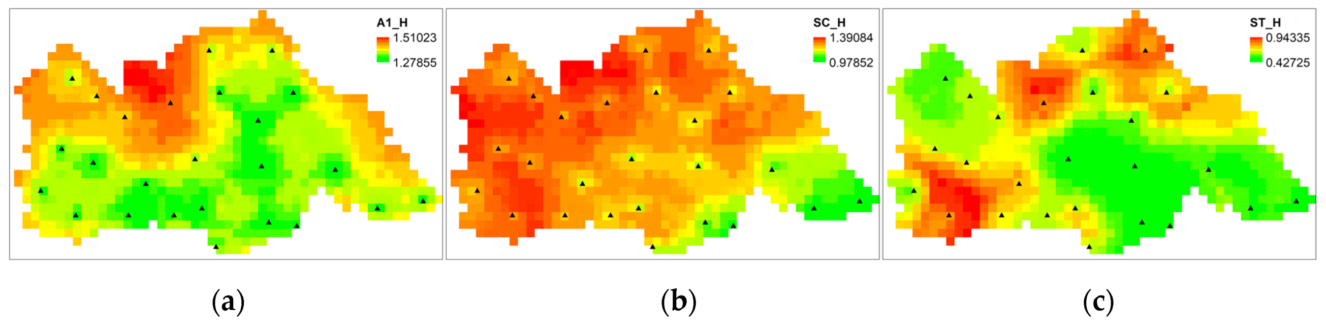
A regional representative network can capture sufficient spatial features. The regional representation of a network here refers to the feature points that contain strong spatial heterogeneity. Different discrete methods will also lead to differences in the spatial distribution of entropy. The three discrete methods have applied the interpolation data of 25 randomly selected points to calculate the distribution of marginal entropy, as shown in Figure 6. In the figure, the spatial difference in marginal entropy calculated by the A1 discrete method is more significant, while the spatial difference in marginal entropy calculated by the SC discrete method is weaker. The overall spatial change in marginal entropy by the three discrete methods is high in the north and low in the south, and the relative elevation of the high-entropy region is also slightly higher.
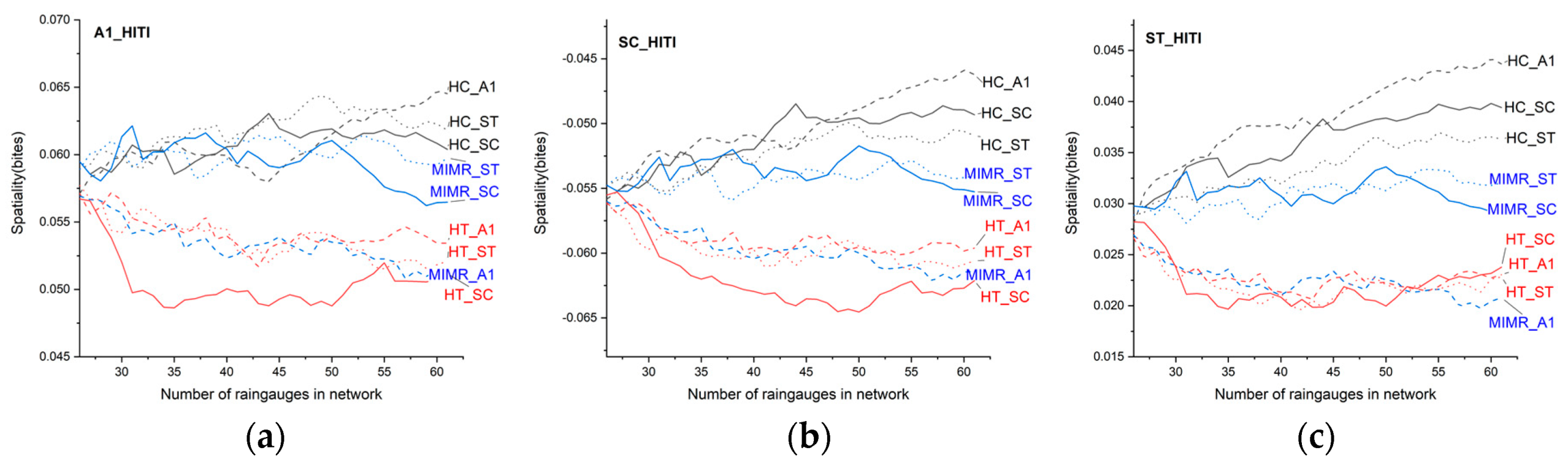
To ensure the objective and credible evaluation of the spatial characteristics of the raingauge network, this paper selects remote sensing data to calculate the spatial indexes to assist in the evaluation of the spatial characteristics of the 9 types of raingauge networks. The spatial index S is calculated based on the marginal entropy and ITI of the pixel and 24 surrounding pixels. The main theoretical basis is to apply local marginal entropy and information flux to express the spatial heterogeneity of a pixel. The spatial importance of the network is better with higher values for the spatial index S. Because there is no way to determine which discrete method has the most reliable spatial property, we calculate the spatial index S of remote sensing data under the three discrete methods. The statistical results of the spatial characteristics of the nine networks are shown in Figure 7.
First, the trends in the evaluation results of the spatial indicators for 9 layouts calculated by different discrete methods are basically the same, which can confirm the objectivity of the spatial nature of the remote sensing data product evaluation network at a certain level.
The spatiality of the HC method results shows the most significant upward trend, especially in the network with 60 rain gauges, regardless of which discrete method was adopted. The results showed the best spatiality. However, the spatiality of the network is not very prominent as a result of the layout having as few networks as possible. The SC method has certain advantages in the layout of a high-density raingauge network. The spatiality of the results of the MIMR method basically remains stable, with no significant upward or downward trend. These results show that the screening conditions of this method balance the spatial relationship to some extent. The results of the HT method have a lower spatiality than those of the other methods, which indicates that this combination of network entropy may focus too much on data with large differences from the original network data, resulting in a uniform distribution of the overall network and the lowest spatiality. In addition, the three discrete methods have significantly different impacts on the spatial performance of the results of the different network design methods. For example, the A1 method has a greater impact on the MIMR layout method, and the spatial performance of the layout results obtained is unsatisfactory.
4.4. Comparison of Accuracy
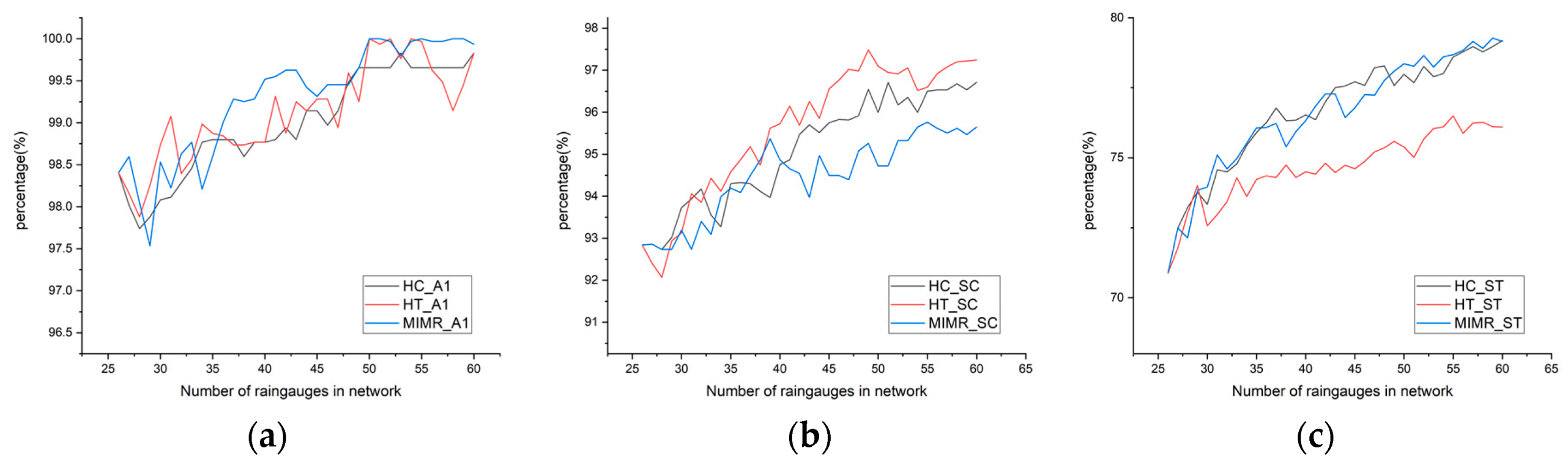
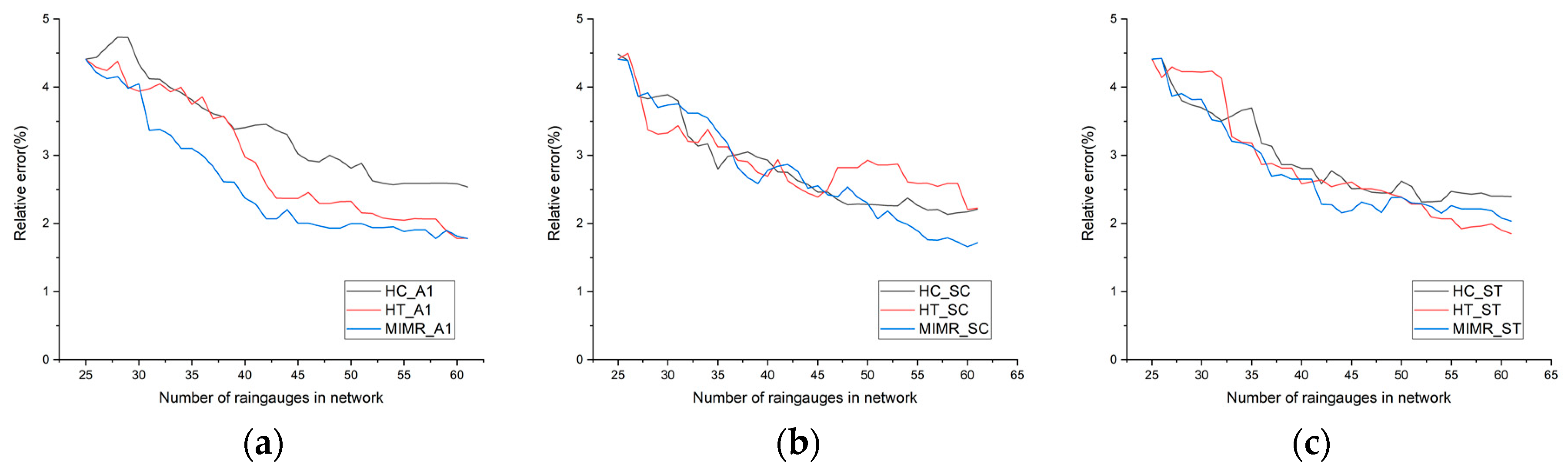
One of the most important evaluation indexes of a network is its accuracy in application. We perform ordinary kriging interpolation for 9 types of networks and compare the interpolation data with the truth value to obtain the relative error in the research area. The results are shown in Figure 8. The statistical results show that the relative error can be reduced from 4.5% to 2.5% in 9 networks with 60 rain gauges.
The rate of accuracy improvement by the A1 discrete method is lower than that by the SC and ST methods, and the error tends to be stable at approximately 45 rain gauges, while the ST and SC methods tend to be stable at 40 rain gauges. This may be because the bin value of the A1 method is too large, resulting in many perturbation factors in the data. In addition, the A1 method has a greater impact on the layout method than the SC and ST methods. The accuracy of the A1 layout method is obviously different, while the layout results of the ST and SC discrete methods are similar when the number of rain gauges is approximately 40 but gradually different when the number of rain gauges is 60. This result shows that the SC and ST discrete methods are more applicable during rainy season rainfall. Compared with the performances of the three layout methods, the accuracy of the MIMR method is better than that of the HC and HT methods in the application of different discrete methods. This result shows that the MIMR method is more applicable to the layout of rain gauges during the rainy season. Among them, the error trend in the MIMR-SC method has been decreasing. Either the number of rain gauges can continue to increase until it reaches a plateau, or the method can be improved to achieve the lowest possible error trend as soon as possible; however, the latter choice has more research prospects.
5. Summary and Conclusions
In this paper, the applications of the A1, ST and SC discrete methods and the HT, HT and MIMR entropy-based design methods are discussed based on the data of rainy season rain gauges and remote sensing products over 10 years. First, the discrete method and entropy target layout method are applied to obtain 9 layout schemes for the research area. Second, the information contents of the site network for the layout results are compared. In terms of numerical value, the order of marginal entropy is A1, SC and ST; that is, the A1 method retains more information than the ST and SC methods. In terms of the proportion of information in the network, the results using the A1 and ST discrete methods have problems, such as the ranges being too high and too low (97.5%–100% and 71%—79%, respectively), compared with the SC method, which is very unfavorable for determining whether the network is in line with the actual application requirements given the information and the objective. Third, the spatial distribution of marginal entropy is compared, and the local marginal entropy and mutual information index calculated by remote sensing data are used to evaluate the spatial performance of the raingauge network. The distribution of marginal entropy calculated by the three discrete methods is significantly different and has the same spatial distribution (high in the north and low in the south), to a certain extent. The spatiality of the results of different layouts has different sensitivities to the choice of discrete method, among which the spatiality of the results of the MIMR method is the most stable compared with that of the HC and HT methods. Finally, the accuracies of the layout results are compared. The accuracy of the A1 discrete method is lower than that of the SC and ST methods. The accuracy of the MIMR method is better than that of the HC and HT methods when different discrete methods are applied. In conclusion, we believe that MIMR combined with the SC discrete method is more suitable for studying the network design of rain gauges during the rainy season.
Taking rainy season precipitation as an example, this study compared the difference between the results of the discrete method and the entropy target. The results of comparisons can provide a valuable reference for station network design with the same hydrological variables. For the station network layouts of various hydrological variables, the comparison process is equally effective. But the conclusions of the comparison will vary due to differences in the spatial correlation degrees of variables. Moreover, the scale of the study area does not directly affect the process of comparisons. In addition, there are still many problems in this paper worthy of further study, such as the relationship between the selection of discrete methods and data characteristics, the relationship between the applicability of the entropy objective algorithm and data characteristics, and whether the application of a multiobjective optimization algorithm to compare discrete methods and entropy objective methods would have the same comparison results.
Author Contributions
Conceptualization, Y.H., H.Z. and Y.J.; Data curation, Y.H. and X.L.; Formal analysis, Y.H. and X.L.; Funding acquisition, H.Z. and Y.J.; Methodology, Y.H.; Project administration, H.Z. and Y.J.; Resources, X.L.; Supervision, Z.H. and H.D.; Validation, Z.H. and H.D.; Writing—original draft, Y.H.; Writing—review & editing, Y.H.
Funding
This research was funded by National Key Research and Development Program of China [No. 2016YFC0401307]; The 13th Five-year Water Program of China [No. 2017ZX07102-001-005] and Basic Scientific Research Special Program of China institute of water resources and hydropower research [No. WR0145B012017].
Conflicts of Interest
The authors declare no conflict of interest.
References
- Apostolidis, N.; Hertle, C.; Young, R. Water recycling in Australia. Water 2011, 3, 869–881. [Google Scholar] [CrossRef]
- Fereidoon, M.; Koch, M.; Brocca, L. Predicting rainfall and runoff through satellite soil moisture data and SWAT modelling for a poorly gauged basin in Iran. Water 2019, 11, 594. [Google Scholar] [CrossRef]
- Van den Honert, R.C.; McAneney, J. The 2011 Brisbane floods: Causes, impacts and implications. Water 2011, 3, 1149–1173. [Google Scholar] [CrossRef]
- Chen, Y.; Shi, P.; Qu, S.; Ji, X.; Zhao, L.; Gou, J.; Mou, S. Integrating XAJ Model with GIUH Based on Nash Model for Rainfall-Runoff Modelling. Water 2019, 11, 772. [Google Scholar] [CrossRef]
- Huang, C.-L.; Hsu, N.-S.; Wei, C.-C.; Luo, W.-J. Optimal spatial design of capacity and quantity of rainwater harvesting systems for urban flood mitigation. Water 2015, 7, 5173–5202. [Google Scholar] [CrossRef]
- Huang, Y.; Chen, S.; Cao, Q.; Hong, Y.; Wu, B.; Huang, M.; Qiao, L.; Zhang, Z.; Li, Z.; Li, W. Evaluation of version-7 TRMM multi-satellite precipitation analysis product during the Beijing extreme heavy rainfall event of 21 July 2012. Water 2014, 6, 32–44. [Google Scholar] [CrossRef]
- Amorocho, J.; Espildora, B. Entropy in the assessment of uncertainty in hydrologic systems and models. Water Resour. Res. 1973, 9, 1511–1522. [Google Scholar] [CrossRef]
- Fattoruso, G.; Longobardi, A.; Pizzuti, A.; Molinara, M.; Marocco, C.; Vito, S.D.; Tortorella, F.; Francia, G.D. Evaluation and design of a rain gauge network using a statistical optimization method in a severe hydro-geological hazard prone area. In AIP Conference Proceedings; AIP Publishing: Melville, NY, USA, 2017; p. 020055. [Google Scholar]
- Moramarco, T.; Barbetta, S.; Tarpanelli, A. From surface flow velocity measurements to discharge assessment by the entropy theory. Water 2017, 9, 120. [Google Scholar] [CrossRef]
- Krstanovic, P.; Singh, V. Evaluation of rainfall networks using entropy: I. Theoretical development. Water Resour. Manag. 1992, 6, 279–293. [Google Scholar] [CrossRef]
- Krstanovic, P.; Singh, V. Evaluation of rainfall networks using entropy: II. Application. Water Resour. Manag. 1992, 6, 295–314. [Google Scholar] [CrossRef]
- Mishra, A.K.; Coulibaly, P. Developments in hydrometric network design: A review. Rev. Geophys. 2009, 47. [Google Scholar] [CrossRef]
- Pathak, S.; Ojha, C.S.P.; Zevenbergen, C.; Garg, R.D. Ranking of Storm Water Harvesting Sites Using Heuristic and Non-Heuristic Weighing Approaches. Water 2017, 9, 710. [Google Scholar] [CrossRef]
- Papana, A.; Kugiumtzis, D. Evaluation of mutual information estimators for time series. Int. J. Bifurc. Chaos 2009, 19, 4197–4215. [Google Scholar] [CrossRef]
- Terrell, G.R.; Scott, D.W. Oversmoothed Nonparametric Density Estimates. J. Am. Stat. Assoc. 1985, 80, 209–214. [Google Scholar] [CrossRef]
- Freedman, D.; Diaconis, P. On the histogram as a density estimator: L 2 theory. Probab. Theory Relat. Fields 1981, 57, 453–476. [Google Scholar]
- Scott, D.W. On optimal and data-based histograms. Biometrika 1979, 66, 605–610. [Google Scholar] [CrossRef]
- Doane, D.P. Aesthetic Frequency Classifications. Am. Stat. 1976, 30, 181–183. [Google Scholar]
- Bendat, J.S.; Piersol, A.G. Measurement and analysis of random data. 1966. [Google Scholar]
- Sturges, H.A. The choice of a class interval. J. Am. Stat. Assoc. 1926, 21, 65–66. [Google Scholar] [CrossRef]
- Singh, V.P. Effect of class-interval size on entropy. Stoch. Environ. Res. Risk Assess. 1997, 11, 423–431. [Google Scholar] [CrossRef]
- Lobbrecht, A.; Price, R.; Alfonso, L. Information theory-based approach for location of monitoring water level gauges in polders. Water Resour. Res. 2010, 46, 374–381. [Google Scholar]
- Li, C.; Singh, V.P.; Mishra, A.K. Entropy theory-based criterion for hydrometric network evaluation and design: Maximum information minimum redundancy. Water Resour. Res. 2012, 48, 5521. [Google Scholar] [CrossRef]
- Fahle, M.; Hohenbrink, T.L.; Dietrich, O.; Lischeid, G. Temporal variability of the optimal monitoring setup assessed using information theory. Water Resour. Res. 2015, 51, 7723–7743. [Google Scholar] [CrossRef] [Green Version]
- Keum, J.; Coulibaly, P. Information theory-based decision support system for integrated design of multivariable hydrometric networks. Water Resour. Res. 2017, 53, 6239–6259. [Google Scholar] [CrossRef]
- Wang, W.; Wang, D.; Singh, V.P.; Wang, Y.; Wu, J.; Wang, L.; Zou, X.; Liu, J.; Zou, Y.; He, R. Optimization of rainfall networks using information entropy and temporal variability analysis. J. Hydrol. 2018, 559, 136–155. [Google Scholar] [CrossRef]
- Yoo, C.; Jung, K.; Lee, J. Evaluation of Rain Gauge Network Using Entropy Theory: Comparison of Mixed and Continuous Distribution Function Applications. J. Hydrol. Eng. 2008, 13, 226–235. [Google Scholar] [CrossRef]
- Alfonso, L.; Lobbrecht, A.; Price, R. Optimization of water level monitoring network in polder systems using information theory. Water Resour. Res. 2010, 46, 595–612. [Google Scholar] [CrossRef]
- Alfonso, L.; He, L.; Lobbrecht, A.; Price, R. Information theory applied to evaluate the discharge monitoring network of the Magdalena River. J. Hydroinformatics 2013, 15, 211–228. [Google Scholar] [CrossRef]
- Leach, J.M.; Coulibaly, P.; Guo, Y. Entropy based groundwater monitoring network design considering spatial distribution of annual recharge. Adv. Water Resour. 2016, 96, 108–119. [Google Scholar] [CrossRef]
- Samuel, J.; Coulibaly, P.; Kollat, J. CRDEMO: Combined regionalization and dual entropy-multiobjective optimization for hydrometric network design. Water Resour. Res. 2013, 49, 8070–8089. [Google Scholar] [CrossRef]
- Chen, Y.-C.; Wei, C.; Yeh, H.-C. Rainfall network design using kriging and entropy. Hydrol. Process. 2008, 22, 340–346. [Google Scholar] [CrossRef]
- Yeh, H.-C.; Chen, Y.-C.; Wei, C.; Chen, R.-H. Entropy and kriging approach to rainfall network design. Paddy Water Environ. 2011, 9, 343–355. [Google Scholar] [CrossRef]
- Yeh, H.-C.; Chen, Y.-C.; Chang, C.-H.; Ho, C.-H.; Wei, C. Rainfall Network Optimization Using Radar and Entropy. Entropy 2017, 19, 553. [Google Scholar] [CrossRef]
- Wei, C.; Yeh, H.-C.; Chen, Y.-C. Spatiotemporal Scaling Effect on Rainfall Network Design Using Entropy. Entropy 2014, 16, 4626–4647. [Google Scholar] [CrossRef] [Green Version]
- Su, H.-T.; You, G.J.-Y. Developing an entropy-based model of spatial information estimation and its application in the design of precipitation gauge networks. J. Hydrol. 2014, 519, 3316–3327. [Google Scholar] [CrossRef]
- Ridolfi, E.; Montesarchio, V.; Russo, F.; Napolitano, F. An entropy approach for evaluating the maximum information content achievable by an urban rainfall network. Nat. Hazards Earth Syst. Sci. 2011, 11, 2075–2083. [Google Scholar] [CrossRef] [Green Version]
- Xu, H.; Xu, C.-Y.; Sælthun, N.R.; Xu, Y.; Zhou, B.; Chen, H. Entropy theory based multi-criteria resampling of rain gauge networks for hydrological modelling – A case study of humid area in southern China. J. Hydrol. 2015, 525, 138–151. [Google Scholar] [CrossRef]
- Xu, P.; Wang, D.; Singh, V.P.; Wang, Y.; Wu, J.; Wang, L.; Zou, X.; Liu, J.; Zou, Y.; He, R. A kriging and entropy-based approach to raingauge network design. Environ. Res. 2018, 161, 61–75. [Google Scholar] [CrossRef] [PubMed]
- Train, K.E. Discrete Choice Methods with Simulation; Cambridge University Press: Cambridge, UK, 2009. [Google Scholar]
- Shannon, C.E. A Mathematical Theory of Communication. Bell Syst. Tech. J. 1948, 27, 623–656. [Google Scholar] [CrossRef]
- Ridolfi, E.; Rianna, M.; Trani, G.; Alfonso, L.; Di Baldassarre, G.; Napolitano, F.; Russo, F. A new methodology to define homogeneous regions through an entropy based clustering method. Adv. Water Resour. 2016, 96, 237–250. [Google Scholar] [CrossRef]
- Cressie, N. The origins of kriging. Math. Geol. 1990, 22, 239–252. [Google Scholar] [CrossRef]
- Hong, Y.; Hsu, K.-L.; Sorooshian, S.; Gao, X. Precipitation Estimation from Remotely Sensed Imagery Using an Artificial Neural Network Cloud Classification System. J. Appl. Meteorol. 2004, 43, 1834–1853. [Google Scholar] [CrossRef] [Green Version]
- Hong, Y.; Gochis, D.; Cheng, J.-T.; Hsu, K.-L.; Sorooshian, S. Evaluation of PERSIANN-CCS Rainfall Measurement Using the NAME Event Rain Gauge Network. J. Hydrometeorol. 2007, 8, 469–482. [Google Scholar] [CrossRef] [Green Version]
- Nguyen, P.; Thorstensen, A.; Sorooshian, S.; Hsu, K.; AghaKouchak, A. Flood Forecasting and Inundation Mapping Using HiResFlood-UCI and Near-Real-Time Satellite Precipitation Data: The 2008 Iowa Flood. J. Hydrometeorol. 2015, 16, 1171–1183. [Google Scholar] [CrossRef]
- Cánovas-García, F.; García-Galiano, S.; Karbalaee, N. Validation of a global satellite rainfall product for real time monitoring of meteorological extremes. In Remote Sensing for Agriculture, Ecosystems, and Hydrology XIX; International Society for Optics and Photonics: Bellingham, WA, USA, 2017; p. 1042109. [Google Scholar]
- Keum, J.; Coulibaly, P. Sensitivity of Entropy Method to Time Series Length in Hydrometric Network Design. J. Hydrol. Eng. 2017, 22, 4017009. [Google Scholar] [CrossRef]
Figure 1.
The study area.

Figure 2.
Marginal entropy statistics based on different discrete methods. (a) Statistical results based on the A1 discrete method; (b) Statistical results based on the SC discrete method; (c) Statistical results based on the ST discrete method.
Figure 2.
Marginal entropy statistics based on different discrete methods. (a) Statistical results based on the A1 discrete method; (b) Statistical results based on the SC discrete method; (c) Statistical results based on the ST discrete method.

Figure 3.
Optimization design results of a network with 60 rain gauges. (a) Network of HC layout method using A1 discrete method; (b) Network of HC layout method using SC discrete method; (c) Network of HC layout method using ST discrete method; (d) Network of HT layout method using A1 discrete method; (e) Network of HT layout method using SC discrete method; (f) Network of HT layout method using ST discrete method; (g) Network of MIMR layout method using A1 discrete method; (h) Network of MIMR layout method using SC discrete method; (i) Network of MIMR layout method using ST discrete method; the black points are existing rain gauges, and colored points are added rain gauges.

Figure 4.
Optimization design results of a network with 40 rain gauges. The descriptions for (a–i) are the same as those in Figure 3.
Figure 4.
Optimization design results of a network with 40 rain gauges. The descriptions for (a–i) are the same as those in Figure 3.


Figure 5.
Comparison of the proportions of network joint entropy. (a) Statistical results of three networks based on the A1 discrete method; (b) Statistical results of three networks based on the SC discrete method; (c) Statistical results of three networks based on the ST discrete method.
Figure 5.
Comparison of the proportions of network joint entropy. (a) Statistical results of three networks based on the A1 discrete method; (b) Statistical results of three networks based on the SC discrete method; (c) Statistical results of three networks based on the ST discrete method.

Figure 6.
The spatial distribution of marginal entropy based on different discrete methods. (a) Statistical results based on the A1 discrete method; (b) Statistical results based on the SC discrete method; (c) Statistical results based on the ST discrete method.
Figure 6.
The spatial distribution of marginal entropy based on different discrete methods. (a) Statistical results based on the A1 discrete method; (b) Statistical results based on the SC discrete method; (c) Statistical results based on the ST discrete method.

Figure 7.
Comparison of network spatiality. (a) Spatial statistics of the A1 discrete method based on remote sensing data; (b) Spatial statistics of the SC discrete method based on remote sensing data; (c) Spatial statistics of the ST discrete method based on remote sensing data.
Figure 7.
Comparison of network spatiality. (a) Spatial statistics of the A1 discrete method based on remote sensing data; (b) Spatial statistics of the SC discrete method based on remote sensing data; (c) Spatial statistics of the ST discrete method based on remote sensing data.

Figure 8.
Comparison of the relative errors of the networks. (a) Statistical results of three networks based on the A1 discrete method; (b) Statistical results of three networks based on the SC discrete method; (c) Statistical results of three networks based on the ST discrete method.
Figure 8.
Comparison of the relative errors of the networks. (a) Statistical results of three networks based on the A1 discrete method; (b) Statistical results of three networks based on the SC discrete method; (c) Statistical results of three networks based on the ST discrete method.


Table 1.
Statistics on the range of entropy.
| Network Design Method | Discrete Method | Joint Entropy of the Network | Marginal Entropy of a Grid | ||||
|---|---|---|---|---|---|---|---|
| Max. | Min. | Range. | Max. | Min. | Range. | ||
| HC | A1 | 3.6353 | 3.5592 | 0.0761 | 1.5102 | 1.2786 | 0.2317 |
| HT | A1 | 3.6506 | 3.5643 | 0.0862 | |||
| MIMR | A1 | 3.6478 | 3.5518 | 0.0960 | |||
| HC | SC | 3.3946 | 3.2550 | 0.1397 | 1.3908 | 0.9785 | 0.4123 |
| HT | SC | 3.4217 | 3.2316 | 0.1901 | |||
| MIMR | SC | 3.3613 | 3.2550 | 0.1063 | |||
| HC | ST | 2.7478 | 2.4598 | 0.2881 | 0.9434 | 0.4273 | 0.5161 |
| HT | ST | 2.6545 | 2.4598 | 0.1947 | |||
| MIMR | ST | 2.7507 | 2.4598 | 0.2910 | |||
© 2019 by the authors. Licensee MDPI, Basel, Switzerland. This article is an open access article distributed under the terms and conditions of the Creative Commons Attribution (CC BY) license (http://creativecommons.org/licenses/by/4.0/).
Share and Cite
MDPI and ACS Style
Huang, Y.; Zhao, H.; Jiang, Y.; Lu, X.; Hao, Z.; Duan, H. Comparison and Analysis of Different Discrete Methods and Entropy-Based Methods in Rain Gauge Network Design. Water 2019, 11, 1357. https://doi.org/10.3390/w11071357
AMA Style
Huang Y, Zhao H, Jiang Y, Lu X, Hao Z, Duan H. Comparison and Analysis of Different Discrete Methods and Entropy-Based Methods in Rain Gauge Network Design. Water. 2019; 11(7):1357. https://doi.org/10.3390/w11071357
Chicago/Turabian StyleHuang, Yanyan, Hongli Zhao, Yunzhong Jiang, Xin Lu, Zhen Hao, and Hao Duan. 2019. "Comparison and Analysis of Different Discrete Methods and Entropy-Based Methods in Rain Gauge Network Design" Water 11, no. 7: 1357. https://doi.org/10.3390/w11071357
Note that from the first issue of 2016, this journal uses article numbers instead of page numbers. See further details here.