New Insights of the Sicily Channel and Southern Tyrrhenian Sea Variability

 ,
, 
 , , , and
Abstract
:1. Introduction
2. Materials and Methods
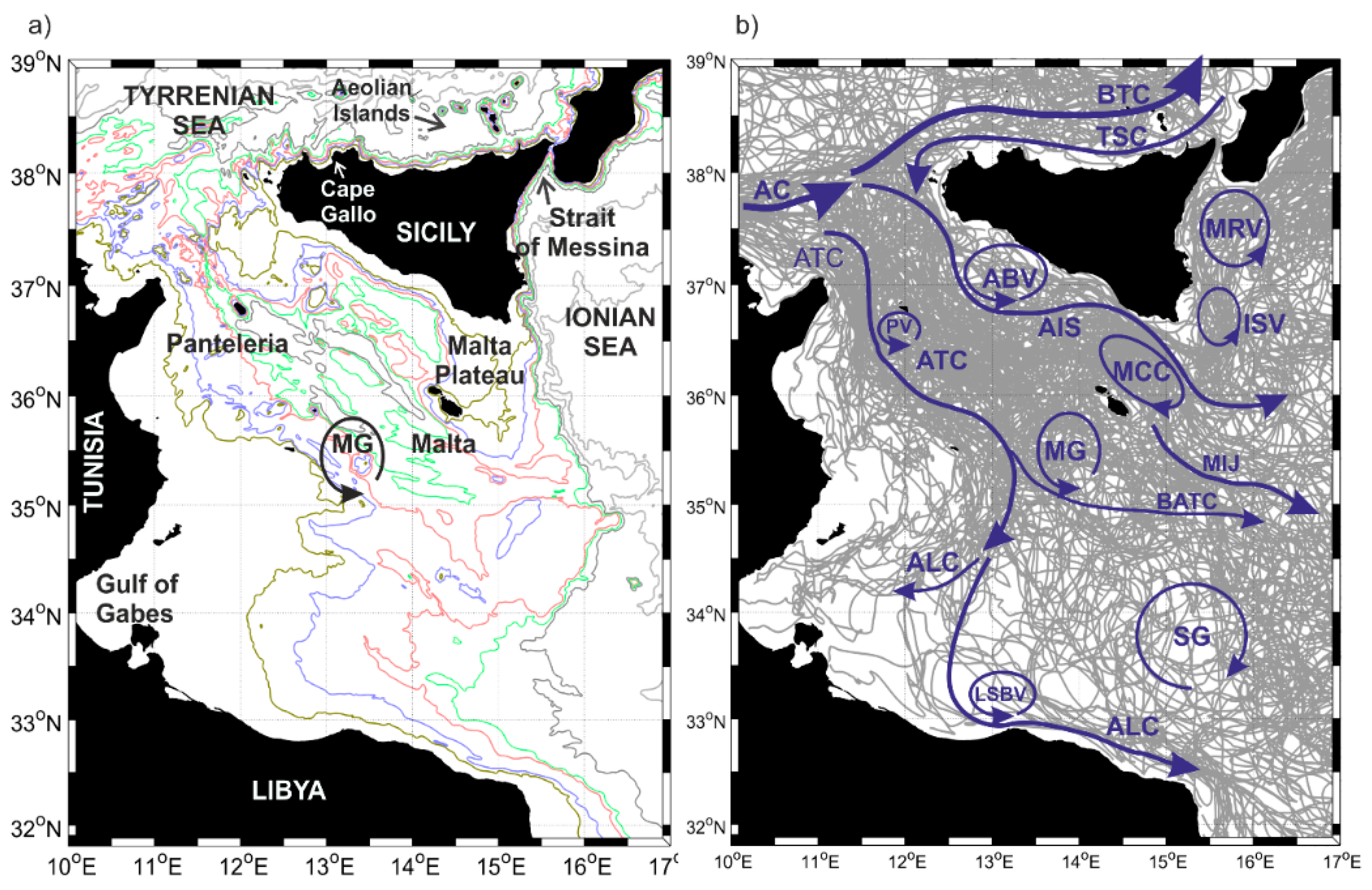
- The OGS Mediterranean drifter dataset in the SC and Southern Tyrrhenian Sea, composed of 377 drifter tracks collected between 1993 and 2018 (Figure 1b). Drifter data were retrieved from the OGS own projects, but also from databases collected by other research institutions and by international data centers (Global Drifter Program, SOCIB, CORIOLIS, MIO, etc.). These data were cleaned of potential outliers and elaborated with standard procedures (editing, manual editing, and interpolation [16,17]). In particular, we use the low-pass filtered and interpolated (6 h) drifter tracks, which represent the near-surface currents between 0 m and 15 m in depth.
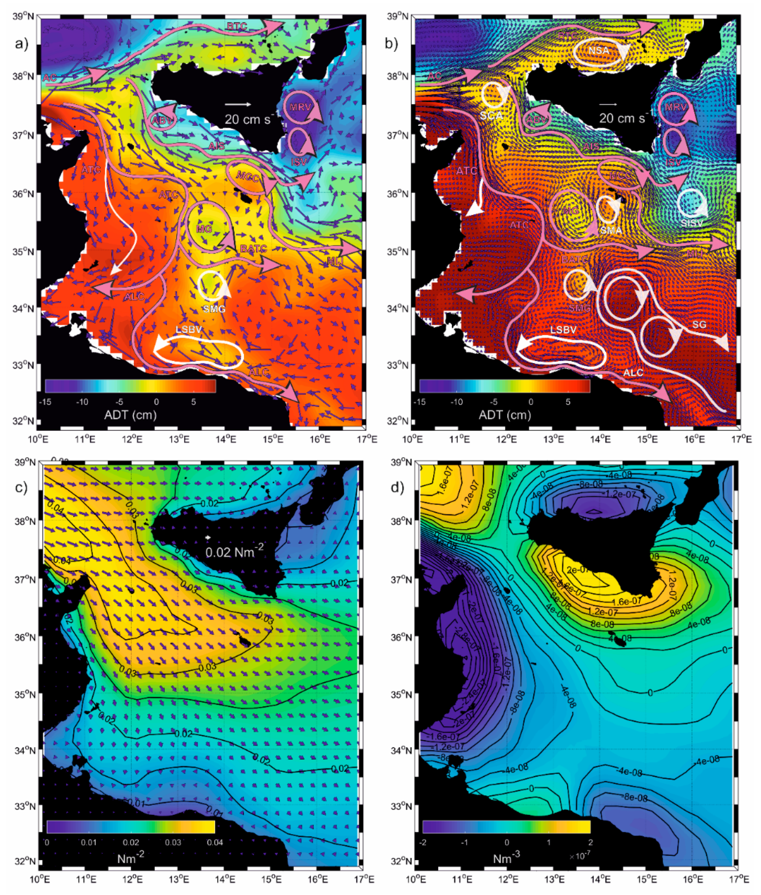
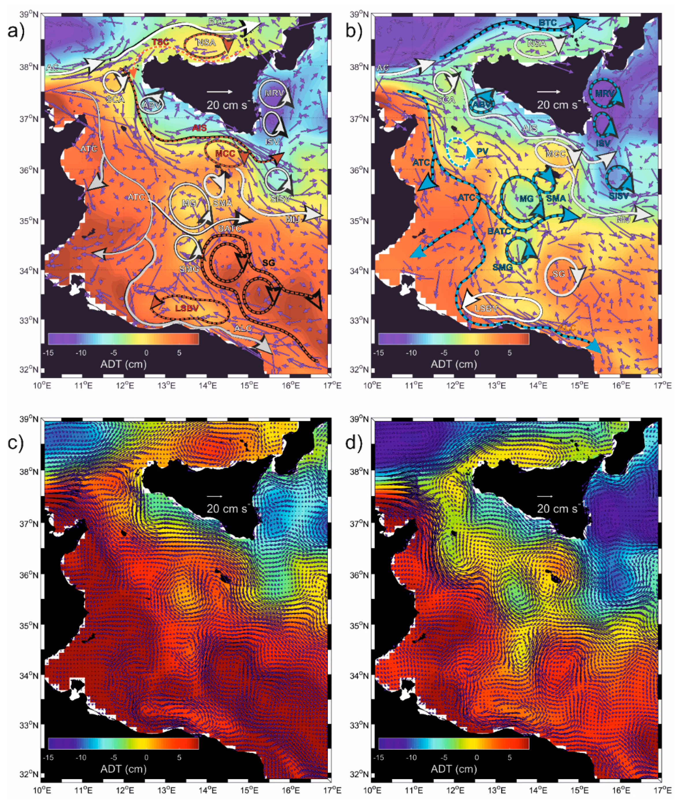
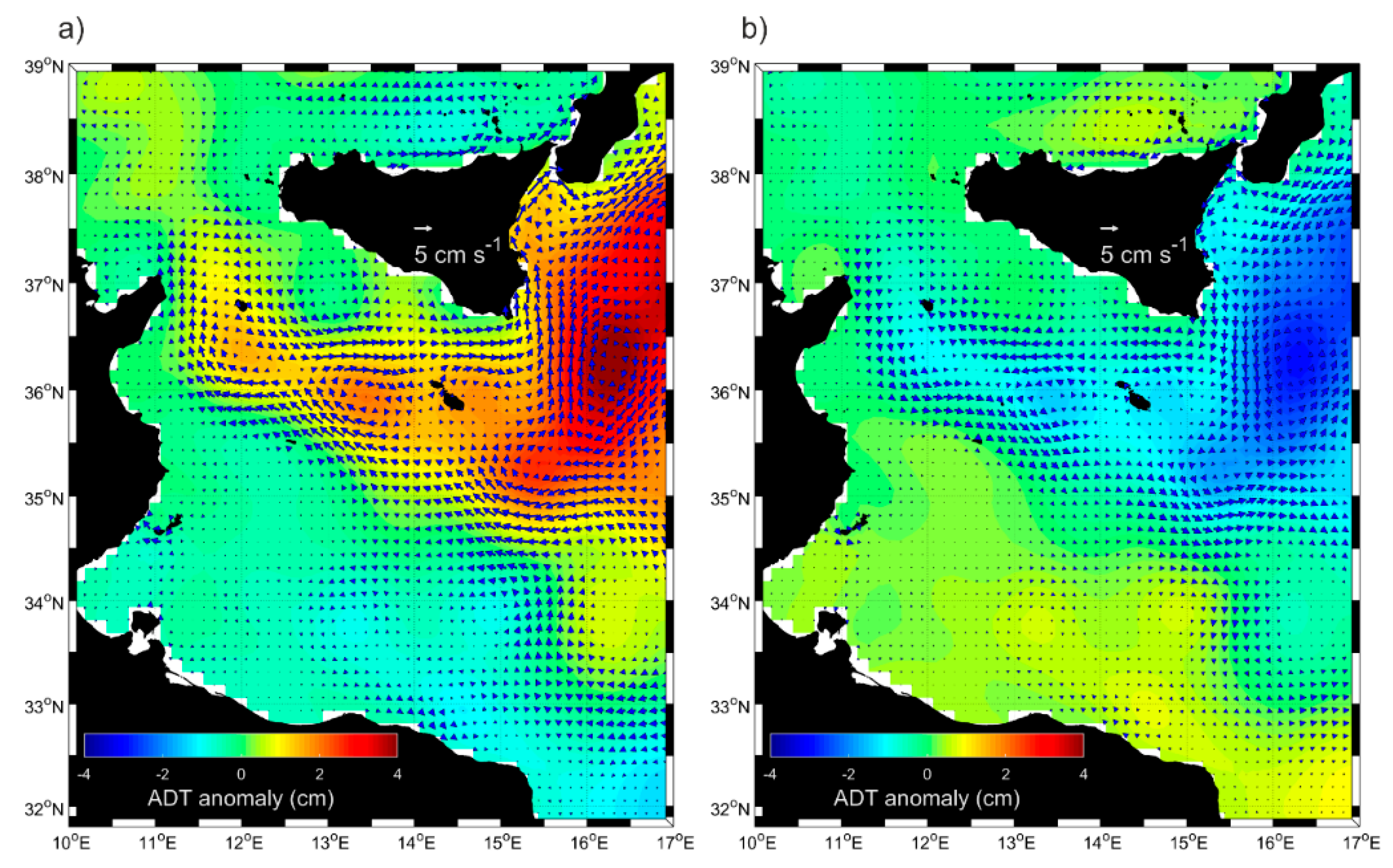
- The daily (1/8° Mercator projection grid) Absolute Dynamic Topography (ADT) and correspondent Absolute Geostrophic Velocities (AGV) derived from altimeter and distributed by CMEMS in the period from 1993 to 2018 (product user manual CMEMS-SL-QUID_008-032-051). The ADT was obtained by the sum of the sea level anomaly and a 20 year synthetic mean estimated in Reference [18] over the 1993 to 2012 period.
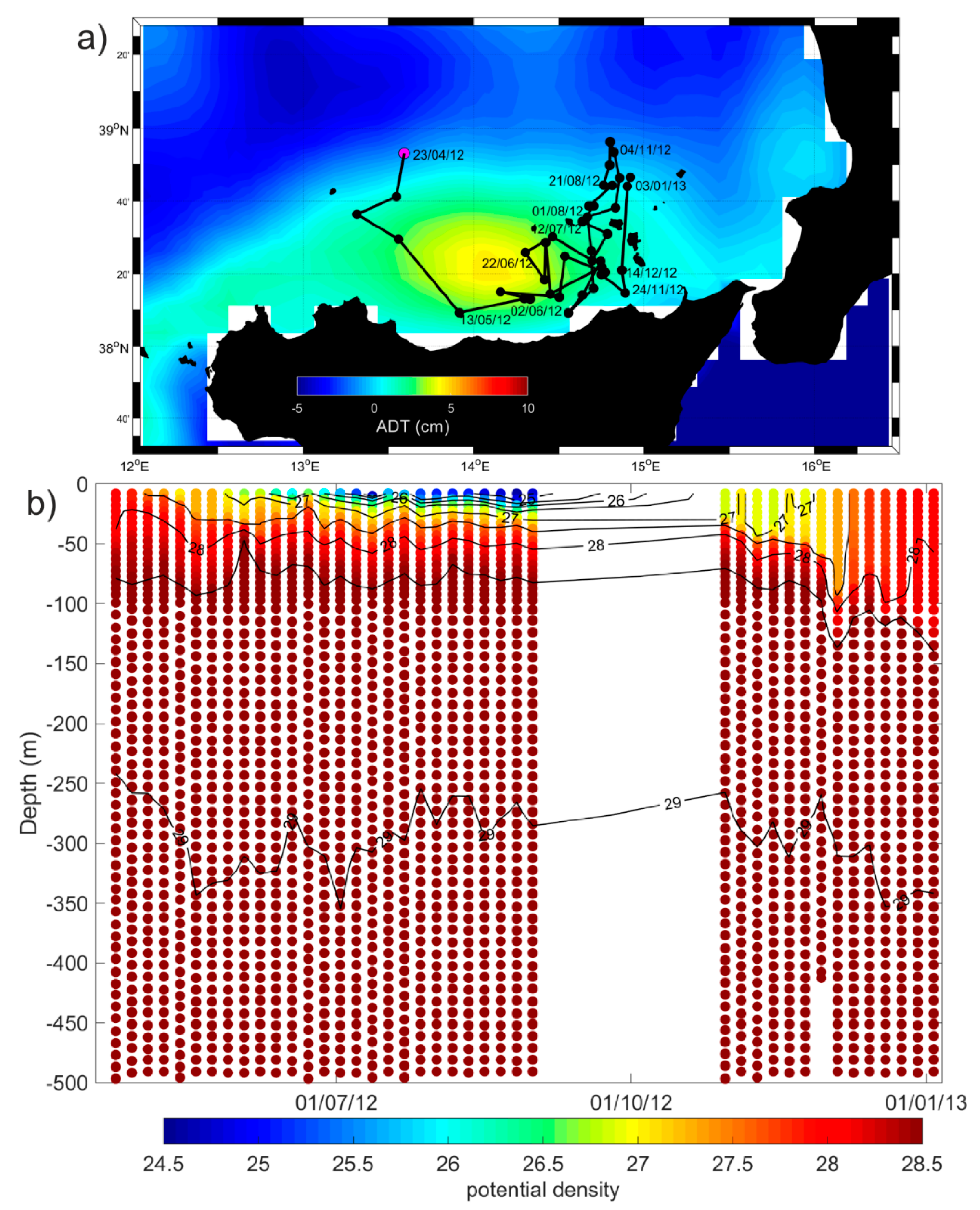
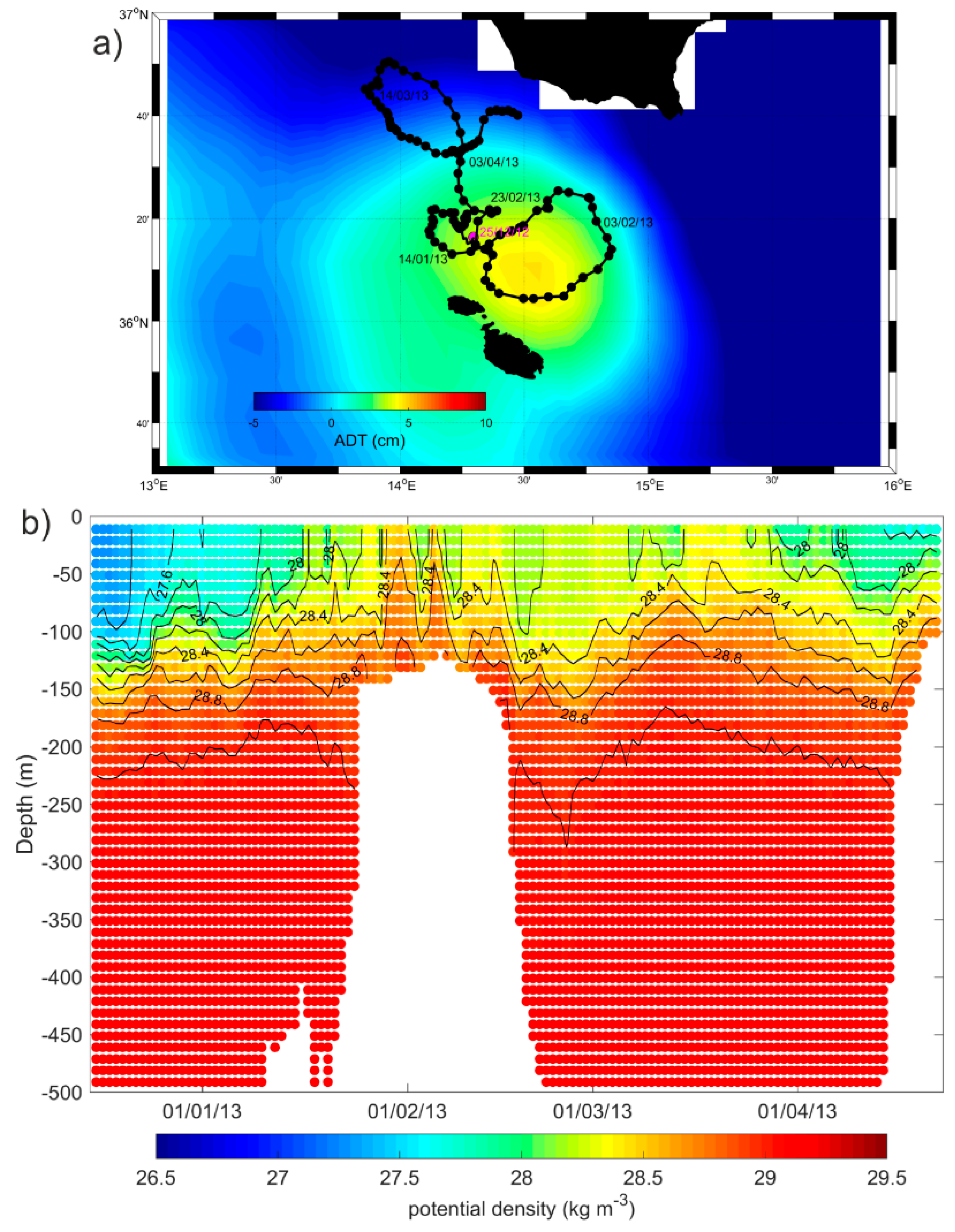
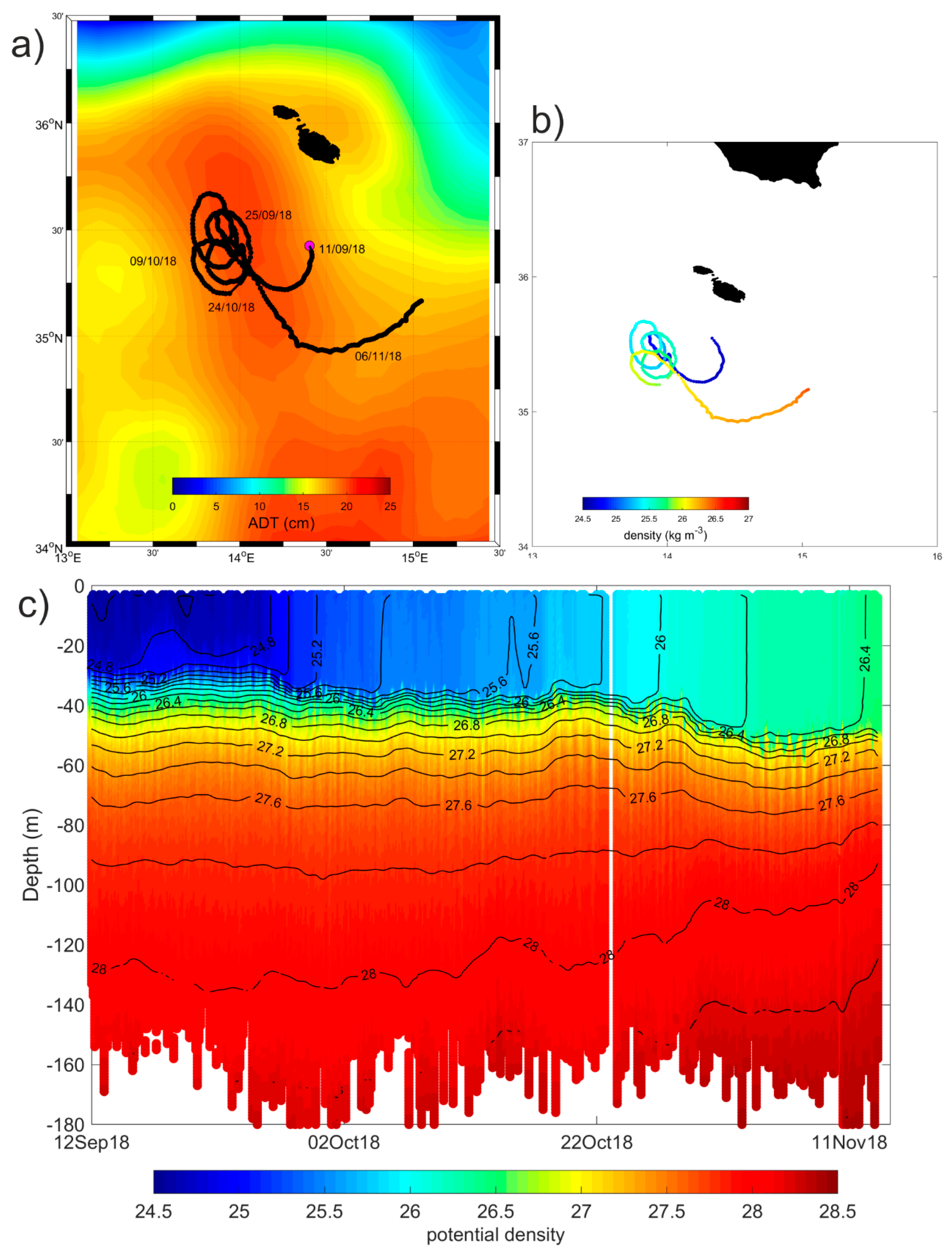
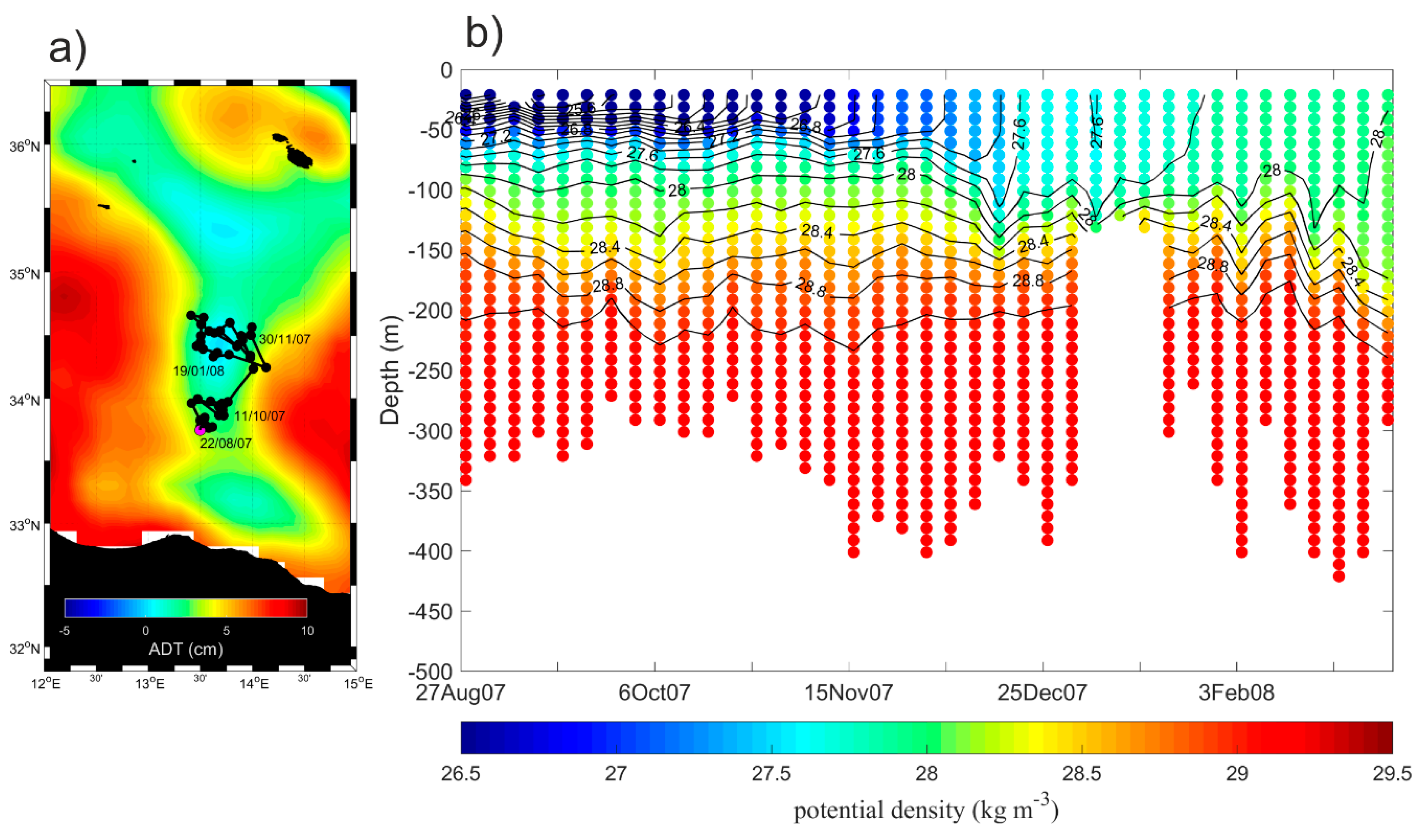
- The Argo float vertical profiles of temperature and salinity from the upper 2000 m of the water column and the horizontal current displacements at the parking depth. In the Mediterranean Sea, the Argo floats are generally programmed to execute 5 day cycles with a drifting depth of 350 m (parking depth). Additionally, they alternate the profiling depth between 700 m and 2000 m (see the MedArgo program in Reference [19]). When a float drifts in a shallow area and touches the ground, it can increase its buoyancy to get away from bottom, or can stay there until it is time to ascent (depending on how it is programmed). Information about grounding events is contained in the Argo float trajectory file. Among all the data available in the Mediterranean Sea, we selected from the part of the Argo floats trajectories which correspond to a float entrapped in the mesoscale structures of the SC and southern Tyrrhenian Sea. These data were used to define the vertical hydrographic peculiarities of the mesoscale features. Details about the missions of the seven floats selected for this work are listed in Table 2.
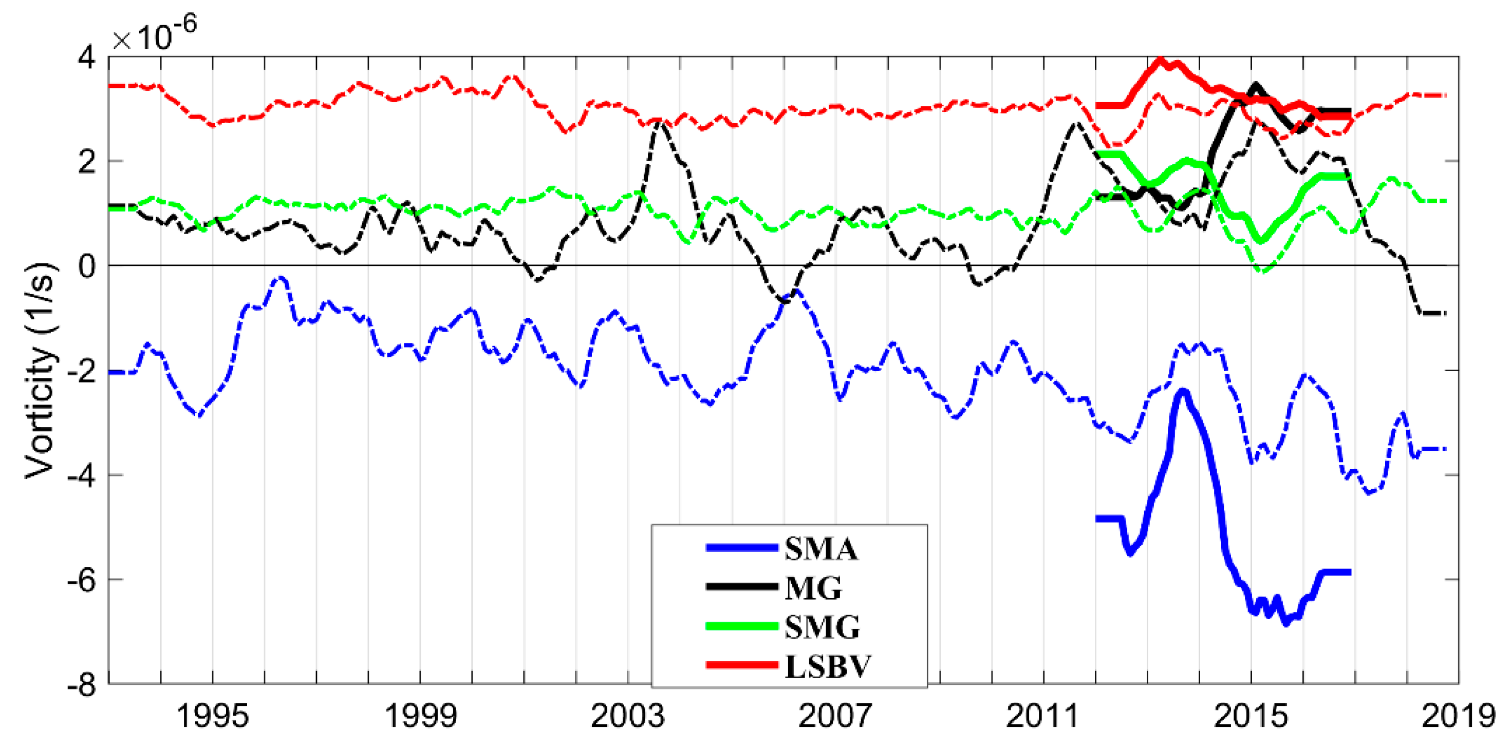
- The optimal currents, estimated by Reference [15] and presently available in the period from 2012 to 2016. This product was used to confirm the occurrence of the mesoscale structure derived from altimetry and to estimate their interannual variability. Indeed, the optimal currents are based on the synergy of the daily 1/8° Copernicus CMEMS altimeter-derived geostrophic velocities (data ID: SEALEVEL_MED_PHY_L4_REP_OBSERVATIONS_008_051) and the daily 1/24° CMEMS sea-surface temperatures for the Mediterranean Sea (data ID: SST_MED_SST_L4_REP_OBSERVATIONS_010_021). The optimal reconstruction method is based on the inversion of the ocean heat conservation equation in the mixed layer [15]. The principles of the optimal currents are thoroughly described in References [15,20,21]. Such a method takes advantage of the high-resolution spatial temporal gradients of the satellite-derived SST to improve the temporal (1 day) and spatial (1/24°) resolution of the altimeter derived geostrophic currents at the basin scale. The reconstruction method of the optimal currents yielded positive improvements for both the components of the motion in the SC [15].
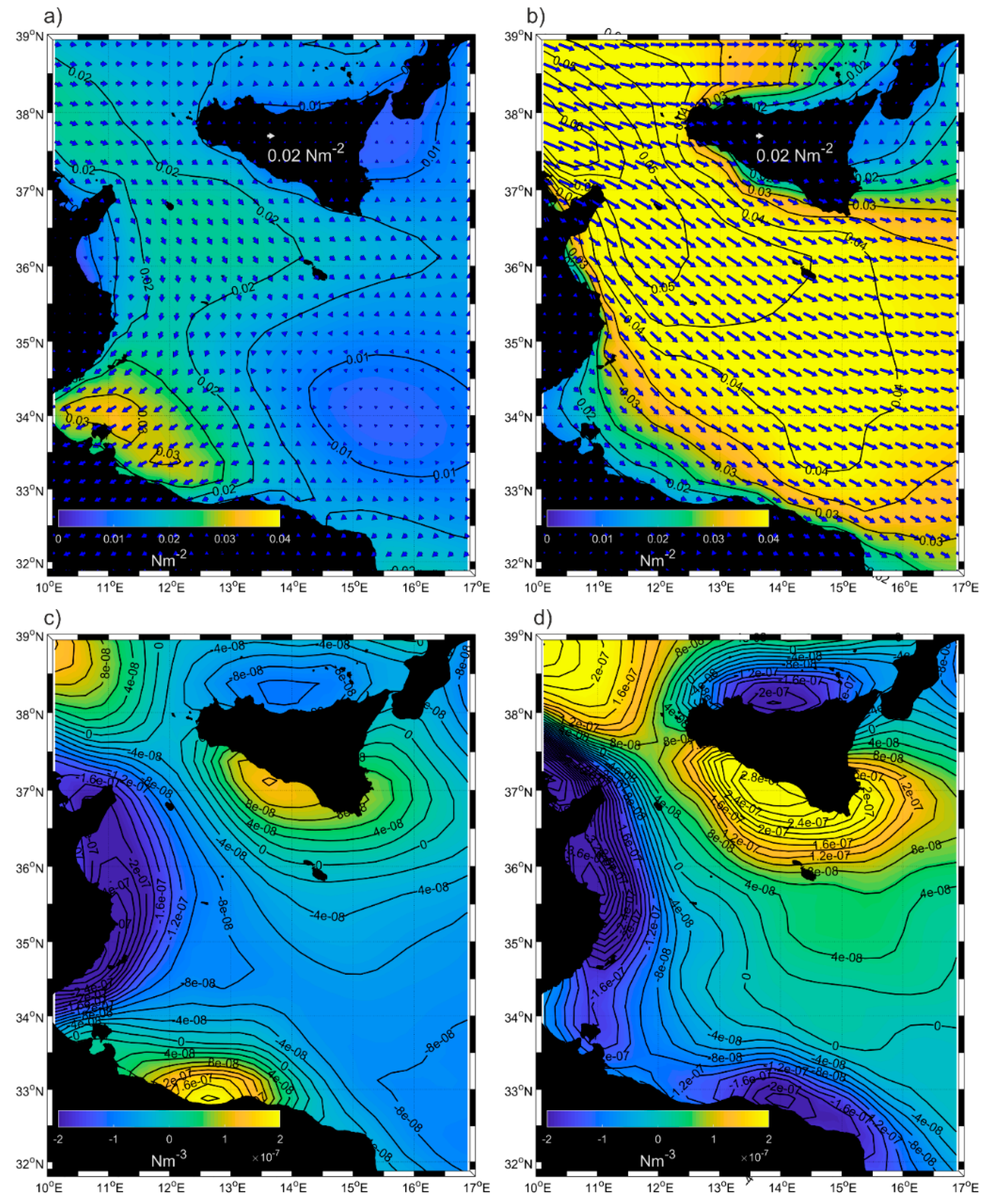
- The Cross-Calibrated, Multi-Platform (CCMP) V2.0 ocean surface wind velocity data, which were downloaded from the NASA Physical Oceanography DAAC for the period from July 1993 to May 2016 [22]. These products were created using a variational analysis method to combine wind measurements derived from several satellite scatterometers and micro-wave radiometers. The temporal resolution of the CCMP product is six hours and the spatial resolution is 25 km (level 3.0, first-look version 1.1).
3. Results
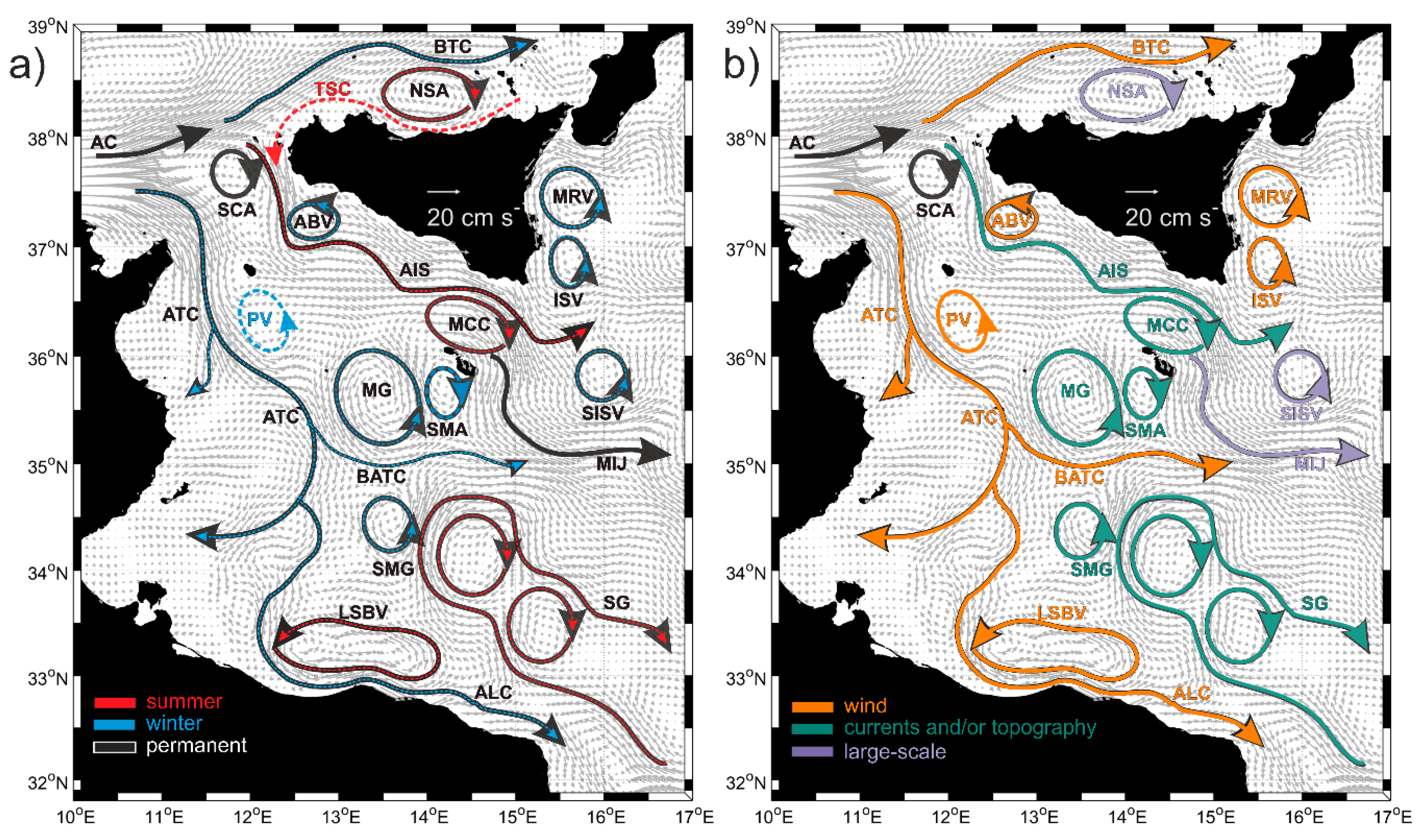
3.1. Mean Currents and Wind Fields
3.2. Seasonal Variability of Currents and Wind Fields
3.3. Decadal Variations
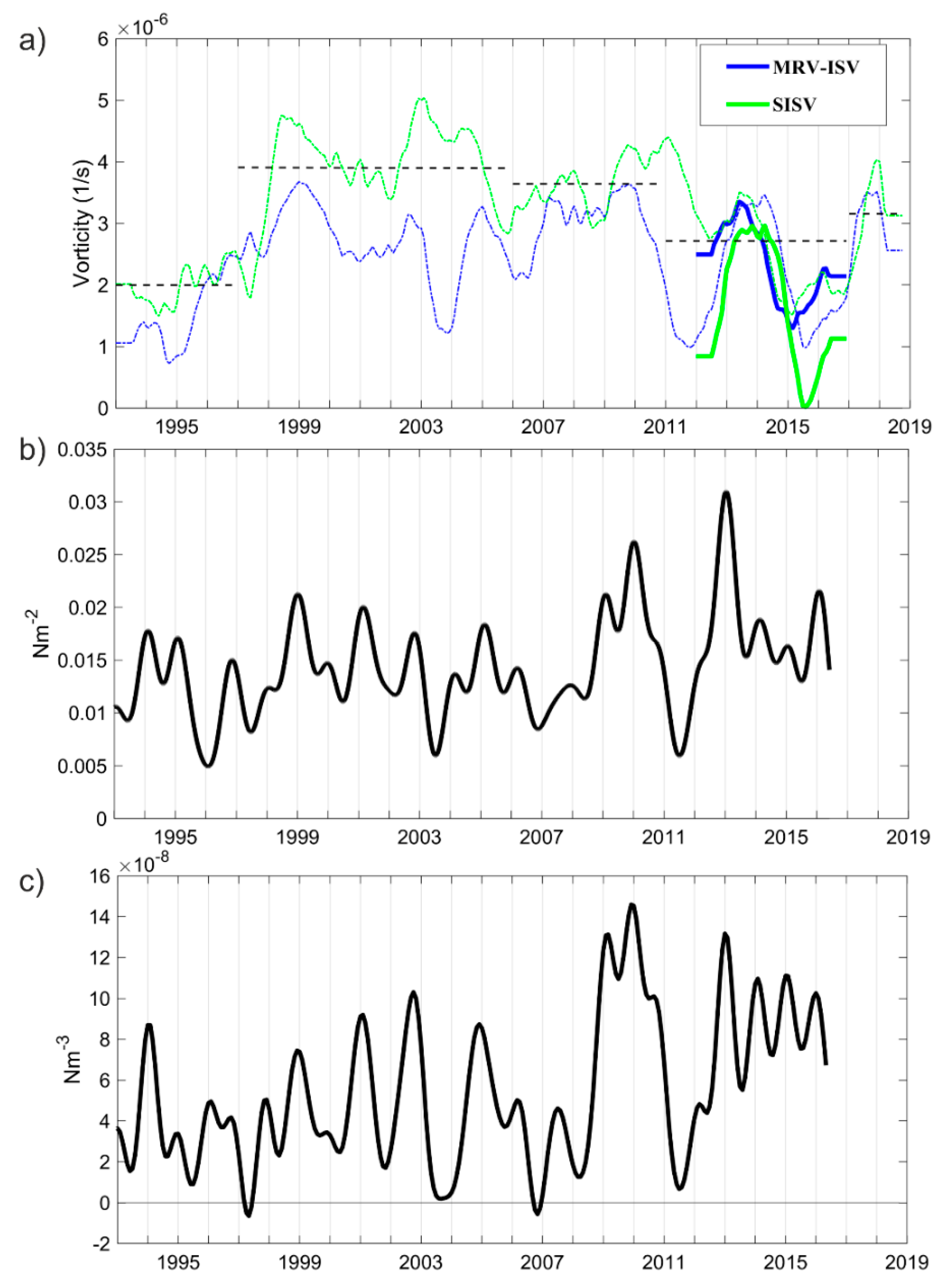
3.4. Interannual Variability and Vertical Structure of the Quasi-Permanent Mesoscale Eddies in the Sicily Channel and Southern Tyrrhenian Sea
3.4.1. Southern Tyrrhenian Sea and Sicily Channel Entrance
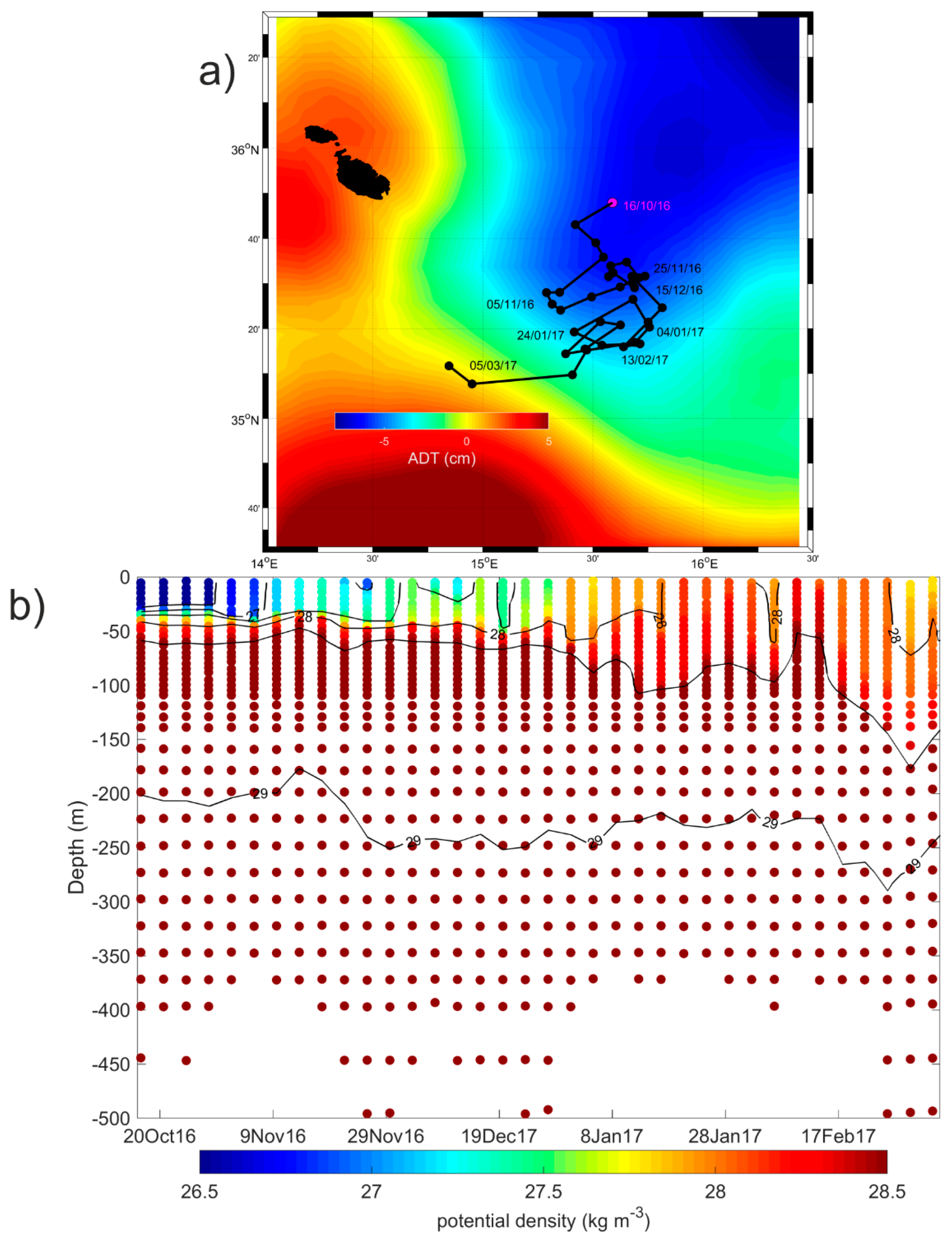
3.4.2. Malta Plateau
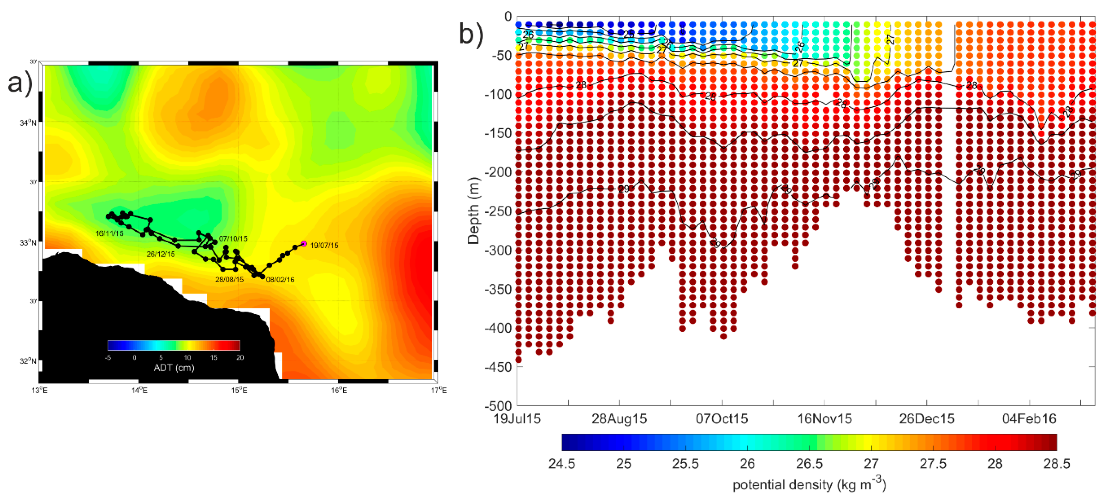
3.4.3. South of Malta
3.4.4. Ionian Cyclones
4. Discussion and Conclusions
Author Contributions
Funding
Acknowledgments
Conflicts of Interest
References
- Sorgente, R.; Olita, A.; Oddo, P.; Fazioli, L.; Ribotti, A. Numerical simulation and decomposition of kinetic energy in the Central Mediterranean: insight on mesoscale circulation and energy conversion. Ocean. Sci. 2011, 7, 503–519. [Google Scholar] [CrossRef] [Green Version]
- Schroeder, K.; Chiggiato, J.; Josey, S.A.; Borghini, M.; Aracri, S.; Sparnocchia, S. Rapid response to climate change in marginal sea. Sci. Rep. 2017, 7, 4065. [Google Scholar] [CrossRef] [PubMed]
- Jouini, M.; Béranger, K.; Arsouze, T.J.; Beuvier, S.; Thiria, M.; Crepon, I.; Taupier-Letage, I. The Sicily Channel surface circulation revisited using a neural clustering analysis of a high-resolution simulation. J. Geophys. Res. Ocean. 2016, 121, 4545–4567. [Google Scholar] [CrossRef]
- Ferron, B.; Bouruet Aubertot, P.; Cuypers, Y.; Schroeder, K.; Borghini, M. How important are diapycnal mixing and geothermal heating for the deep circulation of the Western Mediterranean? Geophys. Res. Lett. 2017, 44, 7845–7854. [Google Scholar] [CrossRef] [Green Version]
- Vladoui, A.; Bouruet-Aubertot, P.; Cuypers, Y.; Ferron, B.; Schroeder, K.; Borghini, M.; Leizour, S.; Ben Ismail, S. Turbulence in the Sicily Channel from microstructure measurements. Deep Sea Res. Part I Oceanogr. Res. Pap. 2018, 137, 97–122. [Google Scholar] [CrossRef]
- Millot, C.; Taupier-Letage, I. Circulation in the Mediterranean Sea. Handb. Environ. Chem. 2005, 5, 29–66. [Google Scholar]
- Lermusiaux, P.F.J.; Robinson, A.R. Features of dominant mesoscale variability, circulation patterns and dynamics in the Strait of Sicily. Deep Sea Res. Part I Oceanogr. Res. Pap. 2001, 48, 1953–1997. [Google Scholar] [CrossRef]
- Béranger, K.; Mortier, L.; Gasparini, G.-P.; Gervasio, L.; Astraldi, M.; Crepon, M. The dynamics of the Sicily Strait: A comprehensive study from observations and models. Deep Sea Res. Part II Top. Stud. Oceanogr. 2004, 51, 411–440. [Google Scholar] [CrossRef]
- Poulain, P.M.; Zambianchi, E. Surface circulation in the central Mediterranean Sea as deduced from Lagrangian drifters in the 1990s. Cont. Shelf Res. 2007, 27, 981–1001. [Google Scholar] [CrossRef]
- Astraldi, M.; Balopoulos, S.; Candela, J.; Font, J.; Gacic, M.; Gasparini, G.P.; Manca, B.; Theocharis, A.; Tintoré, J. The role of straits and channels in understanding the characteristics of Mediterranean circulation. Prog. Oceanogr. 1999, 44, 65–108. [Google Scholar] [CrossRef]
- Poulain, P.-M.; Menna, M.; Mauri, E. Surface geostrophic circulation of the Mediterranean Sea derived from drifter and satellite altimeter data. J. Phys. Oceanogr. 2012, 42, 973–990. [Google Scholar] [CrossRef]
- Pinardi, N.; Zavatarelli, M.; Adani, M.; Coppini, G.; Fratianni, C.; Oddo, P.; Simoncelli, S.; Tonani, M.; Lyubartsev, V.; Dobricic, S.; et al. Mediterranean Sea large-scale low-frequency ocean variability and water mass formation rates from 1987 to 2007: a retrospective analysis. Prog. Oceanogr. 2015, 132, 318–332. [Google Scholar] [CrossRef]
- Molcard, A.; Gervasio, L.; Griffa, A.; Gasparini, G.P.; Mortier, L.; Ozgokmen, T.M. Numerical investigation of the Sicily Channel dynamics: density currents and water mass advection. J. Mar. Syst. 2002, 36, 219–238. [Google Scholar] [CrossRef]
- Amores, A.; Jordà, G.; Arsouze, T.; Le Sommer, J. Up to what extent can we characterize ocean eddies using present day gridded altimetric products? J. Geophys. Res.Ocean. 2018, 123. [Google Scholar] [CrossRef]
- Ciani, D.; Rio, M.-H.; Menna, M.; Santoleri, R. A synergetic approach for the space-based sea surface currents retrieval in the Mediterranean Sea. Remote Sens. 2019, 11, 1285. [Google Scholar] [CrossRef]
- Menna, M.; Gerin, R.; Bussani, A.; Poulain, P.-M. The OGS Mediterranean Drifter Database: 1986–2016; Technical report 2017/92 Sez. OCE 28 MAOS; OGS: Trieste, Italy, 2017. [Google Scholar]
- Menna, M.; Poulain, P.-M.; Bussani, A.; Gerin, R. Detecting the drogue presence of SVP drifters from wind slippage in the Mediterranean Sea. Measurement 2018, 125, 447–453. [Google Scholar] [CrossRef]
- Rio, M.H.; Pascual, A.; Poulain, P.-M.; Menna, M.; Barcelò, B.; Tintorè, J. Computation of a new mean dynamic topography for the Mediterranean Sea from model outputs, altimeter measurements and oceanographic in situ data. Ocean. Sci. 2014, 10, 731–744. [Google Scholar] [CrossRef] [Green Version]
- Poulain, P.-M.; Barbanti, R.; Font, J.; Cruzado, A.; Millot, C.; Gertman, I.; Griffa, A.; Molcard, A.; Rupolo, V.; Le Bras, S.; et al. MedArgo: a drifting profiler program in the Mediterranean Sea. Ocean. Sci. 2007, 3, 379–395. [Google Scholar] [CrossRef] [Green Version]
- Rio, M.H.; Santoleri, R. Improved global surface currents from the merging of altimetry and Sea Surface Temperature data. Remote Sens. Environ. 2018, 216, 770–785. [Google Scholar] [CrossRef]
- Piterbarg, L.I. A simple method for computing velocities from tracer observations and a model output. Appl. Mat. Model. 2009, 33, 3693–3704. [Google Scholar] [CrossRef]
- Atlas, R.; Hoffman, R.N.; Ardizzone, J.; Leidner, S.M.; Jusem, J.C.; Smith, D.K.; Gombos, D. A cross-calibrated, multiplatform ocean surface wind velocity product for meteorological and oceanographic applications. Bull. Am. Meteorol. Soc. 2011, 92, 157–174. [Google Scholar] [CrossRef]
- Shabrang, L.; Menna, M.; Pizzi, C.; Lavigne, H.; Civitarese, G.; Gačić, M. Long-term variability of the southern Adriatic circulation in relation to North Atlantic Oscillation. Ocean. Sci. 2016, 12, 233–241. [Google Scholar] [CrossRef] [Green Version]
- Menna, M.; Reyes Suarez, N.C.; Civitarese, G.; Gacic, M.; Poulain, P.-M.; Rubino, A. Decadal variations of circulation in the Central Mediterranean and its interactions with the mesoscale gyres. Deep Sea Res. Part II: Top. Stud. Oceanogr. 2019, in press. [Google Scholar] [CrossRef]
- Aulicino, G.; Cotroneo, Y.; Lacava, T.; Sileo, G.; Fusco, G.; Carlon, R.; Satriano, V.; Tramutoli, V.; Budillon, G. Results of the first wave glider experiment in the southern Tyrrhenian Sea. Adv. Oceanogr. Limnol. 2016, 7, 16–35. [Google Scholar] [CrossRef]
- Ciappa, A.C. Surface circulation patterns in the Sicily Channel and Ionian Sea as revealed by MODIS chlorophyll images from 2003 to 2007. Contin. Shelf Res. 2009, 29, 2099–2109. [Google Scholar] [CrossRef]
- Rubino, A.; Zanchettin, D.; Androsov, A.; Voltzinger, N.-E. Tidal record as liquid climate archives for large-scale interior Mediterranean variability. Sci. Rep. 2018, 8, 12586. [Google Scholar] [CrossRef]
- Drago, A.; Ciraolo, G.; Capodici, F.; Cosoli, S.; Gacic, M.; Poulain, P.-M.; Tarasova, R.; Azzopardi, J.; Gauci, A.; Maltese, A.; et al. CALYPSO—An Operational Network of HF Radars for the Malta-Sicily Channel. In Proceedings of the Seventh International Conference on EuroGOOS, Lisbon, Portugal, 28–30 October 2014; Dahlin, H., Fleming, N.C., Petersson, S.E., Eds.; EuroGOOS Publication: Brussels, Belgium, 2015. No. 30. ISBN 978-91-974828-9-9. [Google Scholar]
- Capodici, F.; Cosoli, S.; Ciracolo, G.; Nasello, C.; Maltese, A.; Poulain, P.-M.; Drago, A.; Azzopardi, J.; Gauci, A. Validation of HF radar sea surface currents in the Malta-Sicily Channel. Remote Sens. Environ. 2019, 225, 65–76. [Google Scholar] [CrossRef]
- Reyes Suarez, N.C.; Cook, M.S.; Gačić, M.; Paduan, J.D.; Cardin, V. Estimation of sea surface circulation structures in the Malta-Sicily Channel from remote sensing data. Water 2019. under review. [Google Scholar]
- Pinardi, N.; Navarra, A. Baroclinic wind adjustment processes in the Mediterranean Sea. Deep Sea Res. Part II Top. Stud. Oceanogr. 1993, 40, 1299–1326. [Google Scholar] [CrossRef]


| Geographical Names | |
| SC | Sicily Channel |
| Water Masses | |
| AW | Atlantic Water |
| LIW | Levantine Intermediate Water |
| Currents | |
| AC | Algerian Current |
| AIS | Atlantic Ionian Stream |
| ALC | Atlantic Libyan Current |
| ATC | Atlantic Tunisian Current |
| ATC | Atlantic Tunisian Current |
| MIJ | Mid-Ionian Jet |
| BTC | Bifurcation Tyrrhenian Current |
| BATC | Bifurcation Atlantic Tunisian Current |
| TSC | Tyrrhenian Sicilian Current |
| TSC | Tyrrhenian Sicilian Current |
| Gyres and Eddies | |
| ABV | Adventure Bank Vortex |
| ISV | Ionian Shelf break Vortex |
| LSBV | Libyan Shelf Break Vortex |
| MG | Medina Gyre |
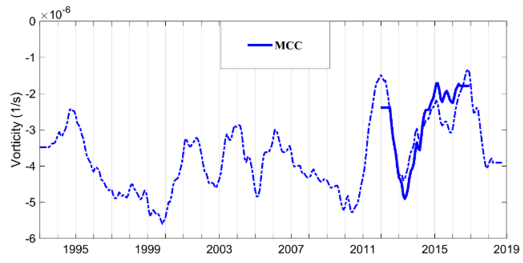
| MCC | Maltese Channel Crest |
| MRV | Messina Rice Vortex |
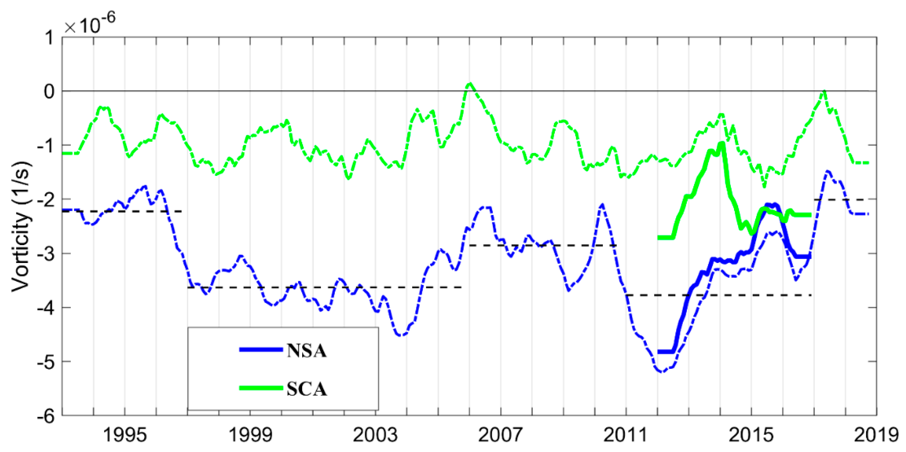
| NSA | Northern Sicily Anticyclone |
| PV | Pantelleria Vortex |
| SCA | Sicily Channel Anticyclone |
| SG | Sidra Gyre |
| SISV | Southern Ionian Shelf break Vortex |
| SMG | Southern Medina Gyre |
| SMA | Southern Maltese Anticyclone |
| Physical Properties | |
| ADT | Absolute Dynamic Topography |
| AGV | Absolute Geostrophic Velocities |
| Float WMO | First Profile | Last Profile | Parking Depth (m) | Profile Depth (m) | Cycle Period (days) |
|---|---|---|---|---|---|
| 6900981 | 23 April 2012 | 3 January 2013 | 350 | 600/2000 | 5 |
| 38.9° N, 13.6° E | 38.8° N, 14.9° E | ||||
| 6901044 | 16 December 2012 | 22 April 2013 | 350 | 700 | 1 |
| 36.3° N, 14.3° E | 36.7° N, 14.5° E | ||||
| 6903242 | 11 September 2018 | 13 November 2018 | 200 | 200 | 0.125 |
| 35.4° N, 14.4° E | 35.2° N, 15.0° E | ||||
| 1900629 | 22 August 2007 | 5 March 2008 | 350 | 700/2000 | 5 |
| 33.7° N, 13.5° E | 34.5° N, 13.9° E | ||||
| 1900948 | 19 July 2015 | 28 February 2016 | 1000 | 1500 | 4 |
| 33.0° N, 15.6° E | 32.9° N, 15.0° E | ||||
| 1900954 | 16 October 2016 | 5 March 2017 | 1000 | 1500 | 4 |
| 35.8° N, 15.6° E | 35.2° N, 14.8° E |
© 2019 by the authors. Licensee MDPI, Basel, Switzerland. This article is an open access article distributed under the terms and conditions of the Creative Commons Attribution (CC BY) license (http://creativecommons.org/licenses/by/4.0/).
Share and Cite
Menna, M.; Poulain, P.-M.; Ciani, D.; Doglioli, A.; Notarstefano, G.; Gerin, R.; Rio, M.-H.; Santoleri, R.; Gauci, A.; Drago, A. New Insights of the Sicily Channel and Southern Tyrrhenian Sea Variability. Water 2019, 11, 1355. https://doi.org/10.3390/w11071355
Menna M, Poulain P-M, Ciani D, Doglioli A, Notarstefano G, Gerin R, Rio M-H, Santoleri R, Gauci A, Drago A. New Insights of the Sicily Channel and Southern Tyrrhenian Sea Variability. Water. 2019; 11(7):1355. https://doi.org/10.3390/w11071355
Chicago/Turabian StyleMenna, Milena, Pierre-Marie Poulain, Daniele Ciani, Andrea Doglioli, Giulio Notarstefano, Riccardo Gerin, Marie-Helene Rio, Rosalia Santoleri, Adam Gauci, and Aldo Drago. 2019. "New Insights of the Sicily Channel and Southern Tyrrhenian Sea Variability" Water 11, no. 7: 1355. https://doi.org/10.3390/w11071355