Simultaneous Sensor Placement and Pressure Reducing Valve Localization for Pressure Control of Water Distribution Systems


1
Process Optimization Group, Institute of Automation and Systems Engineering, Technical University Ilmenau, 98693 Ilmenau, Germany
2
Faculty of Civil and Environmental Engineering Technion—Israel Institute of Technology; Technion City, Haifa 32000, Israel
*
Author to whom correspondence should be addressed.
Water 2019, 11(7), 1352; https://doi.org/10.3390/w11071352
Submission received: 21 May 2019
/
Revised: 24 June 2019
/
Accepted: 25 June 2019
/
Published: 29 June 2019
(This article belongs to the Section Urban Water Management)
Abstract
:Many studies on pressure sensor (PS) placement and pressure reducing valve (PRV) localization in water distribution systems (WDSs) have been made with the objective of improving water leakage detection and pressure reduction, respectively. However, due to varying operation conditions, it is expected to realize pressure control using a number of PSs and PRVs to keep minimum operating pressure in real-time. This study aims to investigate the PS placement and PRV localization for the purpose of pressure control system design for WDSs. For such a control system, a PS should be positioned to represent the pressure patterns of a region of the WDS. Correspondingly, a PRV should be located to achieve a maximum pressure reduction between two neighboring regions. According to these considerations, an approach based on the k-means++ method for simultaneously determining the numbers and positions of both PSs and PRVs is proposed. Results from three case studies are presented to demonstrate the effectiveness of the suggested approach. It is shown that the sensors positioned have a high accuracy of pressure representation and the valves localized lead to a significant pressure reduction.
1. Introduction
Water distribution systems (WDSs) are aimed at supplying consumers’ water demands. Therefore, the water pressure of the system must be stabilized. While a certain pressure must be maintained throughout the network to meet the demand at each location, an excess pressure in water distribution systems often increases leakage and the probability of pipe failure. Such events interrupt the service to consumers and incur high maintenance costs. As such, water leakage control remains one of the biggest challenges in WDS management. In some cities, the non-revenue water (NRW), which is the difference between system input volumes and billed authorized consumptions, may be as high as 40%, of which water loss is one of its most significant parts [1]. Water loss increases significantly as the average system pressure rises. For this reason, pressure control is considered as the most effective mean of diminishing leakage in WDSs, in particular for reducing background leakage, which is the most challenging component of water loss to manage [2]. Moreover, decreasing the operating pressure limit can eliminate the risk of pipe bursts [3]. As a result, WDS pressure measurement and control for the purpose of pressure reduction has become a top priority for water utilities and regulators [4]. A few attempts have been reported for solving those problems. An integral controller and a Smith predictor were used to realize a real-time control system [5]. A model predictive controller was applied in [6,7,8] in an attempt to minimize pressure, energy, and economic costs.
To design a closed-loop pressure control system, a number of pressure sensors (PSs) and pressure reducing valves (PRVs) need to be positioned in the WDS. As only a few PSs and PRVs can be placed in a large network, finding their most effective locations leads to a challenging task. Average zone point (AZP) has been the most common method for positioning PSs. AZP is a point where the pressure variation represents the pressure variations at other points influencing the sum of leak flow rates in the zone as a whole [9]. There are several methods for defining AZP, all are used to calculate the leakage in the WDS. One of the shortcomings of this method is that it needs a lot of flow and pressure sensors to obain data for the calculation of the average value [10]. At the same time, many studies have been made on the placement of PSs to locate leakage using an optimization approach [11,12,13,14]. A method based on the residuals between the pressure measurement and a model-based estimation was presented in the study of Perez et al. [15]. Yoo et al. [16] proposed a pressure driven entropy method that determines a priority order of pressure gauge locations, enabling the impact of abnormal conditions (e.g., pipe failures) to be quantitatively identified in a WDS. Process noise information (i.e., demand fluctuations leading to uncertain pressures at measurement points) was used for PS placement for leakage localization in the work of Steffelbauer et al. [17]. In addition, an entropy-based approach was proposed for sensor placement in urban water distribution networks for the purpose of efficient and economically viable detection of water loss incidents [18]. In the study of Soldevila et al. [19], the sensor placement task was formulated as an optimization problem with binary decision variables solved by a genetic algorithm (GA). Since these methods for sensor placement are mainly for the localization of leakage, they cannot be used for monitoring the real-time pressure aiming at closed-loop pressure control.
A PRV can reduce the pressure of water flowing through it and is commonly used to obtain regulated and constant pressure at its outlet [3]. The optimal location of PRVs has been considered in relation to pressure reduction. An effective way to reduce leakage is to carry out network operational pressure management through optimizing locations and regulations for PRVs [20,21,22]. Hindi and Hamam [23] approximated the PRV localization problem to a mixed-integer linear program (MILP) for one demand pattern. Although the resulting problem can be efficiently solved by an existing MILP solver, the set of links where PRVs are placed must be given a priori. Another disadvantage of this approach is that the linearized model leads to a low accuracy outcome, which may cause an infeasible solution [23]. Araujo et al. [24] developed an optimization approach based on a GA and the EPANET hydraulic simulation model for pressure management. The determination of the number, location, and setting of the valves was formulated as a multi-objective optimization problem with two-criteria. In the first criterion, the number and location of PRVs are predetermined, while for the second criterion, the valve settings are selected to minimize the pressures in the network [25]. Dai and Li [26] proposed a method for solving a mixed-integer nonlinear program (MINLP) problem to identify optimal locations for PRVs in WDSs, resulting in a solution of higher accuracy. The MINLP problem was reformulated as a mathematical program with complementarity constraints (MPCC), which can be efficiently solved using NLP algorithms. The developed method was compared with those in [24,25].
Once PRVs have been installed in a WDS, an operation problem should be considered to determine the setting values of the PRVs. In serveral studies [24,25,27], an evolutionary algorithm based method was used for optimizing the on/off operations of isolated valves to minimize the excessive pressure in a WDS. An extended model for properly describing the three-mode behaviors of PRVs was presented in the study of Dai and Li [28]. This non-smooth model was then smoothed using an interior-point approximation method, so that a continuous optimization problem can be solved by an NLP solver. Although these existing methods can help to optimally place PSs and PRVs separately, as of today, no method is available to simultaneously optimize both, especially for the purpose of designing a closed-loop pressure control system. Real-time pressure control is necessary, since the operating conditions of a WDS change in time due to various reasons (e.g., unpredicted demand modifications). Notably, the placement and operation of PRVs can affect the pressure performance in WDSs. A challenge of the PS system is whether the monitoring accuracy can still be guaranteed when the PRVs operate, or if a pipe burst occurs. As such, PRV localization and PS placement should be considered simultaneously. This implies that sequentially placing PSs after which PRVs are localized can cause unsatisfactory solutions. Therefore, the objective of this study is to develop a simplified approach that is able to simultaneously locate PSs and PRVs for pressure control system design.
To design a closed-loop pressure control system, a number of PSs and PRVs need to be positioned in the WDS. On the one hand, the measurement using a small number of PSs should represent the pressure behavior of the whole network. On the other hand, the whole network pressure should be reduced at a maximum level by a small number of PRVs. The basic idea of this work is to identify both the number and the positions of PSs and PRVs by classifying the water network into pressure regions using a clustering method. Because of its simplicity of implementation and high efficiency for handling large data sets, the k-means algorithm is the most widely used clustering method [29,30,31]. The centers of a given number of clusters are determined by minimizing the mean squared distance from each data point to its nearest center. k-means was extended to k-means++ by a randomized seeding method to improve its speed as well as accuracy and to avoid a local solution [32,33]. The gap statistic is a well-known method to determine the number of clusters [34]. Its basic idea is to compare the curve of the within-clusters homogeneity from the original data with that of its expected value, assuming that the data follow a uniform distribution. A weighted gap statistic was proposed to improve the accuracy of the clustering [35]. Based on these methods, a simple approach is developed to simultaneously localize PSs and PRVs in this study. After determining the number of sensors, an identical number of regions of the network will be defined, with each region containing one sensor representing the pressure behavior of the region. Then, the PRVs will be localized at the edges of the regions because of the maximum pressure difference on those edges. The results of three case studies demonstrate the applicability of this approach.
The remainder of this paper is organized as follows. In Section 2, an approach for pressure sensor placement is proposed. Section 3 presents the method for the localization of PRVs. Section 4 describes the numerical implementation of the whole approach. In Section 5, the approach is demonstrated on three benchmark WDSs. Section 6 concludes the paper.
2. Pressure Sensor Placement
2.1. Problem Description
The objective of PS placement for designing a pressure control system is to select sensor positions at which the measurement can represent the pressure behaviors of the whole network with a few sensors. However, because of the complexity of a WDS, many sensors may be required for a high degree of representation. From another perspective, monitoring the pressure change is more important for the purpose of control. Therefore, we use the pressure change to evaluate the pressure behavior at a node and its relation to those at the other nodes of a region. Clearly, if the pressure curves over time at all, nodes would change with the same rates and patterns, and one pressure sensor at any position could be enough to singlehandedly predict the pressure change in the entire WDS. However, due to the varying head loss in the pipes and different water demands at nodes, differences of rate changes as well as patterns of pressure curves at different nodes can be significant.
Thus, we propose to divide a WDS into several regions based on the pressure curves at the nodes. One PS should be installed in each defined region to monitor the pressure change at the node and to represent the pressure changes at the other nodes in the region where the sensor is installed. The number of PSs can be determined by the number of regions reflecting different pressure patterns of the WDS. Thus, an approach is developed by evaluating the accuracy of the representation, in order to find a minimum number of sensors and their locations so that they can accurately represent the pressure changes in the WDS.
2.2. The K-Means++ Method to Determine the Regions
The aim of this subsection is to partition a WDS into several regions with similar pressure curves. For this purpose, we divide the pressure curves at all nodes of a WDS into several groups according to their changing rates, by using cluster analysis. The goal of cluster analysis is to cluster different objects into groups which are as similar as possible after the division is made.
The k-means algorithm [29,30] is one of the most commonly used methods for grouping objects [31]. It is a typical distance-based clustering algorithm in which the distance is used as the evaluation index of similarity. The closer the distance between two objects, the greater their similarity is. This algorithm is able to determine, from a set of similar objects with a predefined number of groups, a respective center for each cluster. The k-means algorithm is an efficient method that can handle many different data types, with a low computation expense. Thus, it is suitable for clustering vast datasets [29,30].
For a set of n-observations, k-means aims to partition these observations into K (<n) clusters. The procedure consists of the following steps [30]:
- Randomly select K points as starting centers of the clusters.
- Allocate the data points to the nearest clusters based on their distance from the center.
- The mean of each of the K clusters becomes the new center.
- Repeat from step 2 until the locations of the centers do not change.
Now, we use this method to determine K pressure regions and their centers as positions for placing the PSs. For a WDS with n nodes, we initially run the EPANET model to obtain pressure curves at the nodes over a fixed time period m (e.g., 24 h). We denote the pressure curve as with the unit of meter (m), , where i is the sampling time point, j is the index of the node, and l is the index of the cluster. Thus, the distance of to the center of the lth cluster is defined as:
where is the pressure value at the center of the lth cluster. The pressure curves are now allocated to different clusters (regions) based on the distance values. Then, the new centers of the clusters will be updated based on the average value of the pressure curves inside the individual regions as follows:
This process will repeat until the update of the centers converges to an allowed threshold. In this way, the WDS is divided into K pressure regions with their center nodes representing the pressure behaviors of the individual regions. Therefore, the pressure sensors should be placed at these center nodes to monitor the pressure changes in their corresponding regions.
However, besides its simplicity and high efficiency for handling large data sets, the k-means method has two limitations:
- The number of clusters needs to be given a priori, which is a difficult task in practice.
In many cases, it is the most appropriate to determine the number of clusters depending on the network itself.
In the context of the PS placement, the first limitation may lead to cluster centers close to each other. If sensors placed at these cluster centers are too close to each other, the resulting control system will have a poor performance due to the coupling of the measured signals. To the second limitation, a clustering method is needed to determine a minimum number of sensors which can represent the pressure behaviors of the whole WDS.
The k-means method was extended to k-means++ to overcome the first limitation. k-means++ selects K cluster centers at the beginning according to the following rational: select the first cluster center randomly, then select the second cluster center at a node with a farther distance from , and the third cluster center at a node with a farther distance from . This procedure continues until [32,33]. In this way, k-means++ ensures that once the cluster centers are selected, the corresponding pressure sensors will be as far as possible from each other, thus avoiding a local clustering solution.
However, similar to the k-means method, the number of clusters K has to be defined by the user in K-means++. To solve this problem, we use the method of gap statistic, as described in the following subsection.
2.3. Determining the Number of Clusters K
Occasionally, the number of clusters K can be derived from the constraints of the system itself. For example, K may be predetermined if the WDS manager would like to allocate an exact number of pressure sensors. However, in many cases, the number of sensors cannot be specified a priori and thus an algorithm should be employed to determine a proper K. In this study, we use an improved gap statistic to address this issue.
The gap statistic [34] is a method which provides the number of clusters in a data set. Suppose that we have clustered the data into K clusters. The sum of the pairwise distances for all nodes in cluster l is as follows:
where and are pressure values at nodes and in time , respectively. The total average distance for all K clusters is:
where is entitled the total within intra-cluster variation [34]. Gap statistic aims to standardize the comparison of with a null reference distribution of the data, i.e., a distribution without obvious clustering. The estimate for an optimal number of clusters K is the value at which falls the farthest below the reference curve. is interpreted as a log-likelihood [36]. This information is contained in the following expression for the gap statistic:
where is the expectation under a sample of size N from the reference distribution, is the total within intra-cluster variation of the reference distribution. In [34], it was proposed that a uniform distribution is used for the reference distribution. However, it is well-known that a uniform distribution will be considered if no knowledge regarding the randomness of the process is available. However, the node pressure curves of a WDS have a periodic regular pattern, meaning that their changing rate, which is important for the reference distribution, is not a random number.
Therefore, we propose a method to generate a suitable reference distribution for clustering pressure regions of a WDS as follows. For a clearer description, we express the data of the pressure curves of the WDS in a matrix form, i.e., X is a pressure matrix. Using a singular value decomposition X = and a transformation = XV, we can compute , which represents the rate of the pressure change. The reason of employing instead of X, is that it takes into account the shape of the data distribution and makes the procedure rotationally invariant, as long as the clustering method itself is invariant [34]. Based on a matrix will be determined as follows:
where and are the minimum and maximum value of in the i-th row, which are the same as the minimum and maximum value of in the i-th row. The reference data sets are generated by sampling uniformly in the range of and which are the lower and upper bouds of the original data set. At the same time, it can be seen from Equation (6) that the derivative of each column of at any time point has the same sign as that of . This ensures that the value of is within a reasonable range and has the same change rate with . Finally, a back-transformation is performed via Z = to generate the reference distribution Z.
The quality of the sampled distribution for the gap statistic is assessed as follows:
where is the average value and the standard deviation of , respectively. is the standard error of the generated reference distribution. B is the number of the generated reference distributions. In general, more precise results can be achieved with a larger B.
As a result, the optimal number of clusters K is determined as the smallest k, so that ≥ [34]. However, the way the number K is determined here, might be too small to guarantee the accuracy of the representation for the clustered centers to reflect the pressure behavior of the individual regions. In addition, the number of K may change after each run of the algorithm. Therefore, for the sensor placement, we propose to choose the number of K at the maximum value of Δ, where Δ = . In our case studies described in Section 5, it is shown that this modified method yields more accurate results in less computation time.
2.4. The Accuracy of Representation (AOR)
2.4.1. Definition of AOR
After determining the number of regions (Section 2.3) and the cluster centers (Section 2.2), it is necessary to evaluate the quality of these decisions. As mentioned before, the most important quality criterion for sensor placement in a WDS, for the purpose of control system design, is their ability to represent the pressure change in the monitored region. We define the degree of such representation as the accuracy of representation (AOR) as follows. Consider region l, the relative pressure change rate at time point i and node j is:
and the value at the sensor:
The AOR at each node is defined as:
This leads to a matrix denoting the AOR values for all nodes and time periods in region l:
According to Equation (12), an AOR value equal to 1.0 means that the sensor can completely represent the pressure change at time i and node j. If the AOR value deviates from 1.0, the representation is degraded. Therefore, the nodes with the values in Equation (13) in a small neighborhood around 1.0, e.g., , are highly represented by the sensor at the related time points. Then, the AOR of region l, , is defined as the ratio of the total number of the values in the range of [0.8, 1.2] to the total number of the elements in Equation (13):
The AOR of the whole network is:
is a percentage value between 0% and 100% describing the performance quality of the PSs in the WDS. For instance, if , it means that 90% of the pressure change rate values at all nodes of the WDS in the considered time horizon can be represented by the PSs placed using the clustering method.
2.4.2. Improving the AOR with a Partition Matrix
A pressure change at a node can be represented by multiple sensors. However, in the above discussed clustering method, the coupling effect for the representation between the sensors is not considered. Considering the coupling effect should enhance the precision of AOR. For this purpose, we employ the idea of introducing a partition matrix in the fuzzy k-means method [37]. A partition matrix a matrix consisting of its elements expressed as:
where is the pressure curve at node and are the pressure curve at the center of cluster l and c, respectively, and [0, 1]. In fact, the value of describes the membership function. The value of s in Equation (16) determines the property of the method. When s1, will be 0 or 1, which implies that the method reduces to K-means++. In the fuzzy K-means, s is commonly set to 2. As a result, the AOR is now calculated as:
Using this method, it is shown that the AOR of the whole network can be improved according to the numerical experiments in the case studies in Section 5.
3. Localization of PRVs
3.1. Pressure Analysis on the Edges of the Regions
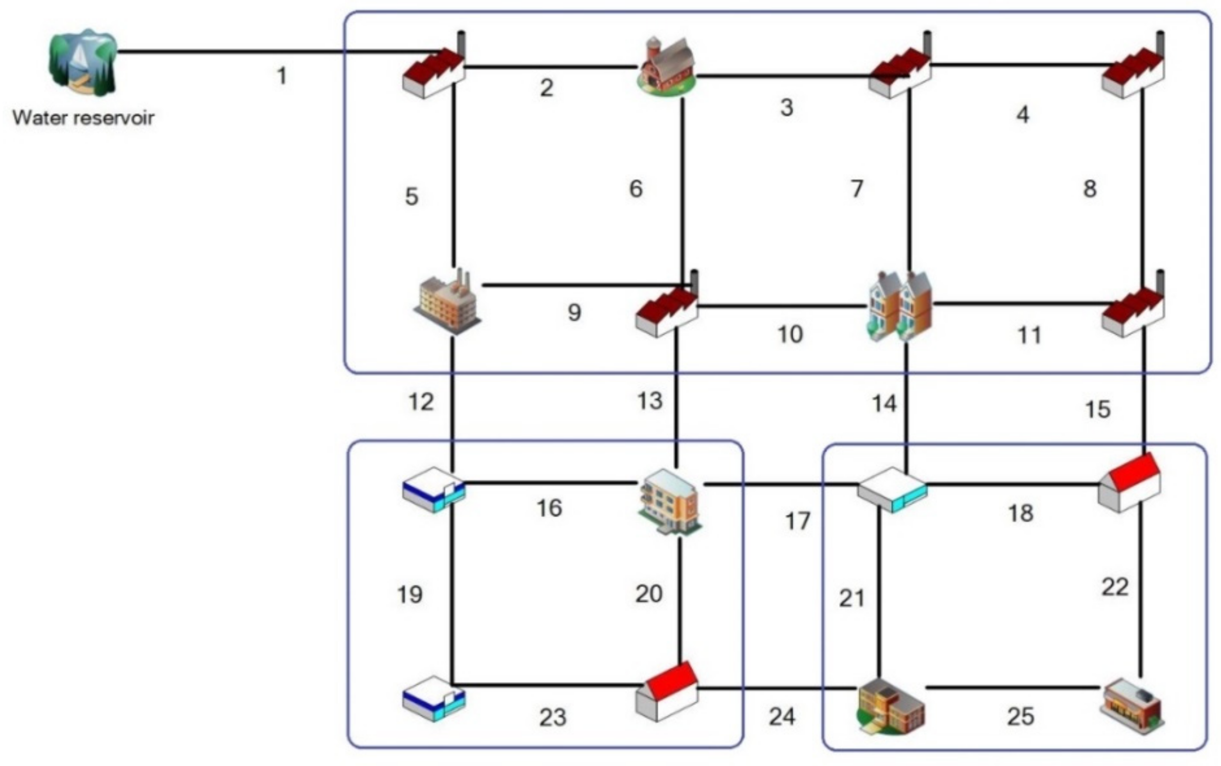
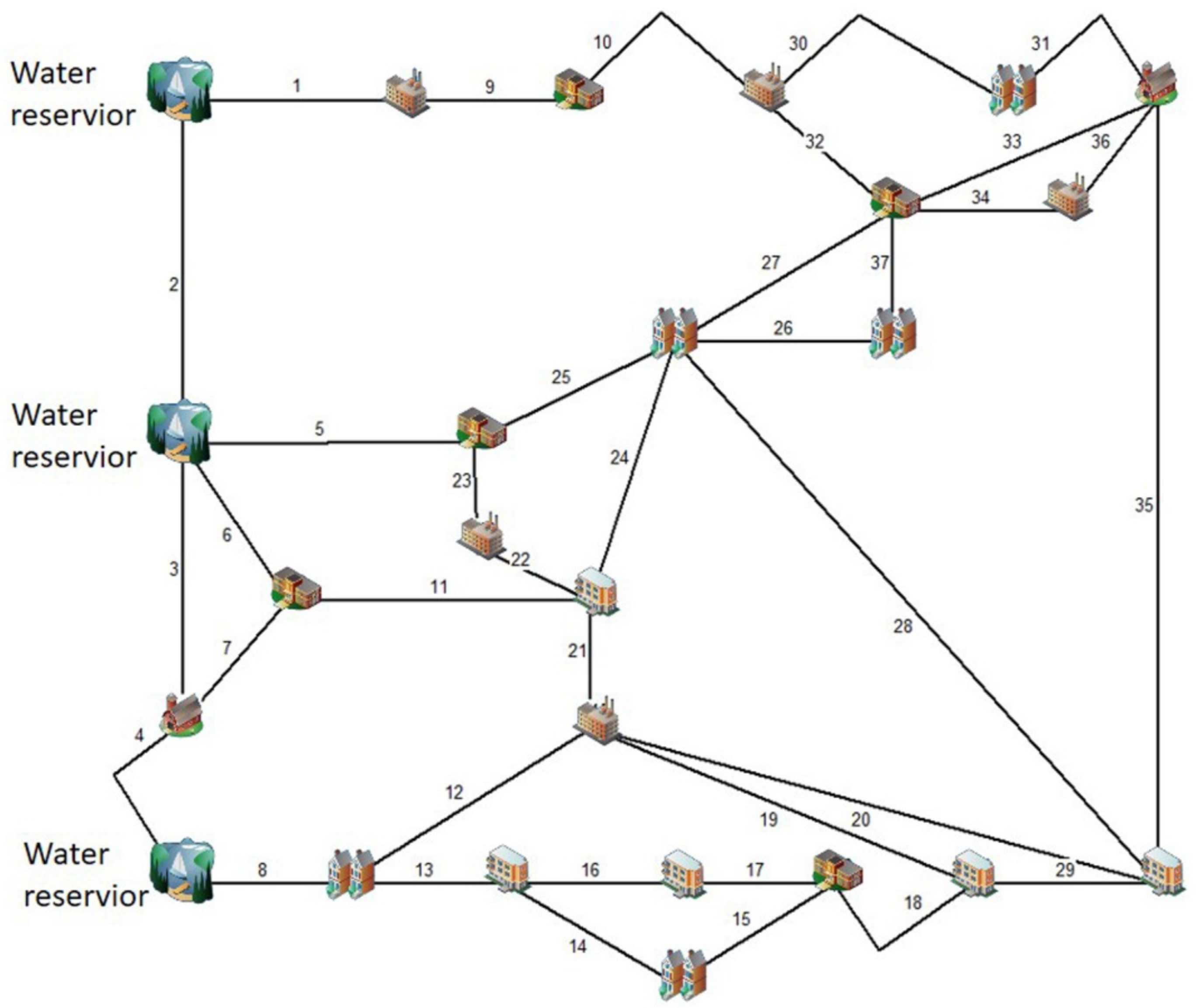
In Section 2, we use a clustering method to classify the network into several pressure regions. As a result, the pressure at the nodes in a region is distinguished from that at the nodes in another region. This means that there will be a distinct pressure difference between two neighboring regions, and this difference is higher than that between two nodes inside a region. Therefore, we propose to localize the PRVs at the edges between adjacent regions. For instance, Figure 1 shows a network which is divided into three regions by the clustering method. It is seen that pipes 8, 17, 13, 16, 10, 21 are on the edges of the regions. The head loss at these pipes should be higher than those on the pipes inside the regions.
Another advantage of placing PRVs at the edges of the regions is that the PRVs are far away from the sensors. When a PRV is installed on a pipe, the head loss of the pipe and the pressure curve at the downstream nodes will be changed, and thus the AOR in this region and even in the adjacent region will diminish. Therefore, if the PRVs are placed at the region edges, their distance to the sensors will be larger and thus their influence on the precision of AOR will be less.
3.2. Placement of the PRVs
In the previous subsection, we elaborated on why valves should be placed at the regions edges. The presence of a PRV increases the head loss across its link and thus reduces the pressure at downstream nodes [38]. This subsection will discuss in which pipes along the region’s edges the valves should be placed. The external pressure will be greatly reduced by inserting a valve on a pipe with the highest pressure difference between the up- and downstream area. This is because the potential pressure reduction in such conditions is higher than that of pipes with a smaller pressure difference. From the pressure control point of view, a PRV is used to release pressure at its downstream nodes. A high-pressure difference between the up- and downstream nodes is required to ensure the quality of the pressure control. According to these considerations, the following rules are used for PRV placement:
- Since a PRV works with its water flow only in one direction, a pipe in which the water flow direction alters during the operation should not be selected for the valve placement. Otherwise, there will be no assurance to meet the pressure demand.
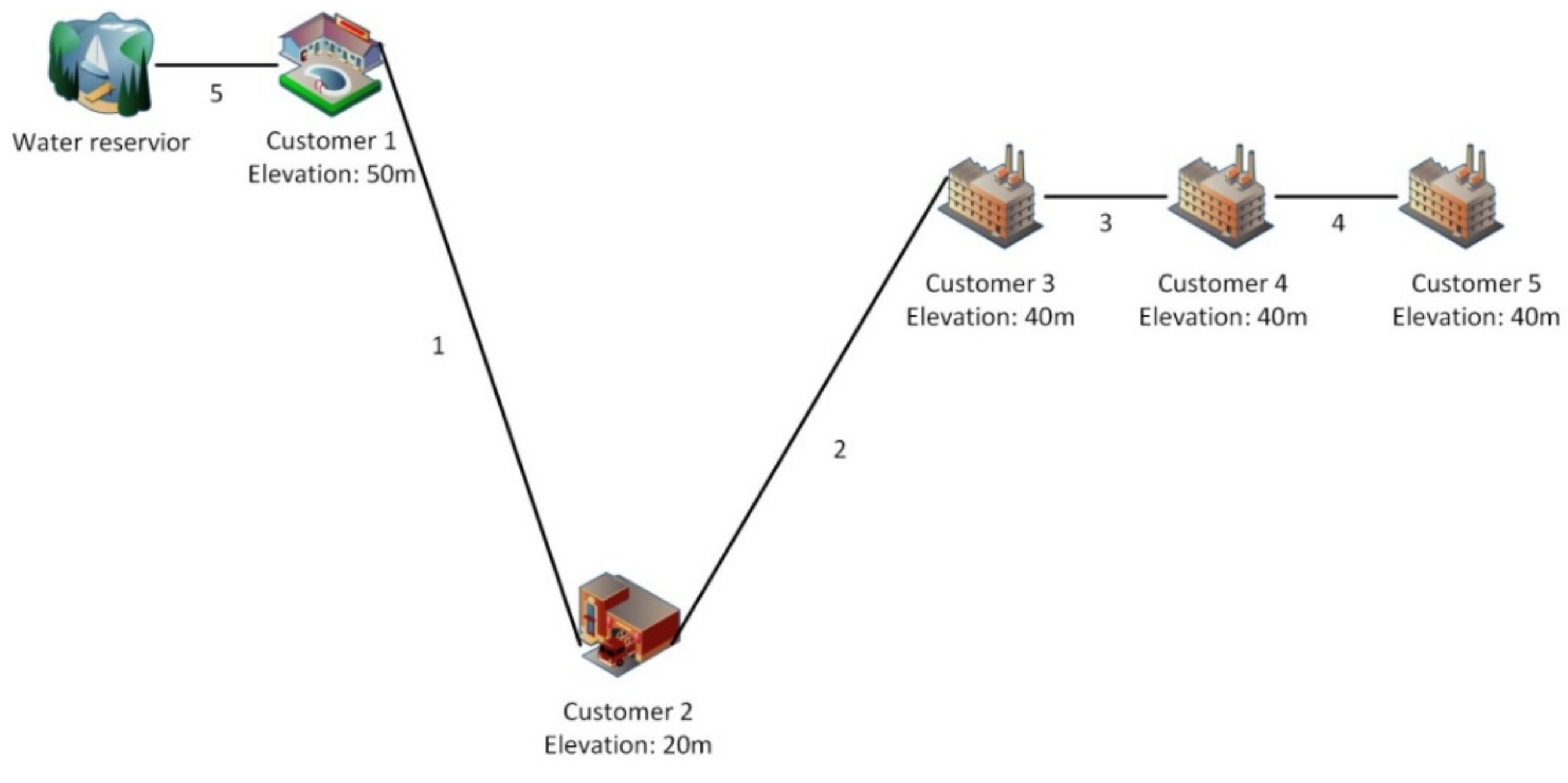
- For PRV placement, the downstream elevation should be considered to ensure the pressure demand at the downstream nodes. For example, if the main source of pressure difference is from the elevation difference, and if a downstream node is lower in elevation, its pressure will usually be greater than the upstream pressure. In this case, if the PRV is placed on this link due to the large pressure difference, the pressure at the downstream nodes can be lower than the pressure demand.For example, as shown in Figure 2, the elevations at nodes 1, 2, 3, 4 and 5 are 50 m, 20 m, 40 m, 40 m and 40 m, respectively. Node 2 is the downstream node of pipe 1 and the upstream node of pipes 2, 3 and 4. A PRV may be installed on pipe 1 and its setting of the valve is determined to reduce the external pressure at node 2 so that the pressure meets the lowest pressure requirement at node 2. Then, the head of node 2 will be lowered, and therefore, the minimum pressure requirement for nodes 3, 4 and 5 may not be met. Thus, a PRV should not be installed on pipe 1, in spite of its high pressure difference.
- Pipes directly connected to a water tank or a pump should not be selected as candidates for placing PRVs. This is due to the fact that the elevation generated by a water tank or a pump is the only energy source ensuring the consumer demands. Installing a valve there may degrade proper delivery of the water to some consumers.
We use an iterative procedure to localize PRVs one by one. After a PRV placed into the WDS, it will have an effect on the AOR of the PSs. Therefore, we run k-means++ once again to update the division of the pressure regions. More PRVs will cause higher pressure reduction. Still, at the same time, as the number of PRVs increases, their marginal benefit to the total pressure reduction will be decreased. Therefore, when the decrease of the total pressure is insignificant by adding a new PRV, the current number can be chosen as the number of PRVs required.
3.3. Determining the Setting Values for PRVs
The setting value of a PRV is a preset pressure value on its downstream side. It plays an important role in the operation of the valve. A PRV has three different operating states [38]:
- Partially opened (active mode): water flows through the valve and the downstream pressure is reduced to the setting value of the PRV, when the upstream pressure is above the setting value.
- Fully open (open mode): the PRV is entirely open and acts as if it is not present, when the upstream pressure is below the setting value.
- Fully closed (closed mode): the PRV closes completely and acts as a check valve, when the pressure on the downstream side exceeds that on the upstream side, or if reverse flow in the pipe is incipient.
For the pressure computation, we need to determine the setting values of the PRVs to be placed in the WDS. Using our iterative approach, after a PRV is localized, the setting value of the PRV needs to be determined, since it has an effect on the placement of the next valve. The setting value should be determined so that the total excess pressure of the whole network is minimized. At the same time, the minimum pressure requirement at each node is ensured during operation. This leads to a constrained optimization problem. The objective function is defined as the minimization of the sum of the pressures at all nodes in the considered time period:
subject to the constraints of the node pressure and the setting value of the PRVs:
where is the setting value of PRVs, is the number of PRVs to be installed in WDS. Equation (20) means that, to guarantee the pressure constraints in the WDS, the setting value must be higher than , which is the lowest pressure demand in WDS. is the upper bound of the , which should be the highest pressure in the time horizon of the upstream node of the PRV. This is because when the PRV setting value is higher than the highest pressure of the upstream node, this PRV will always work at the open mode. Then, the installation of this PRV makes no sense.
4. Implementation of the Proposed Approach
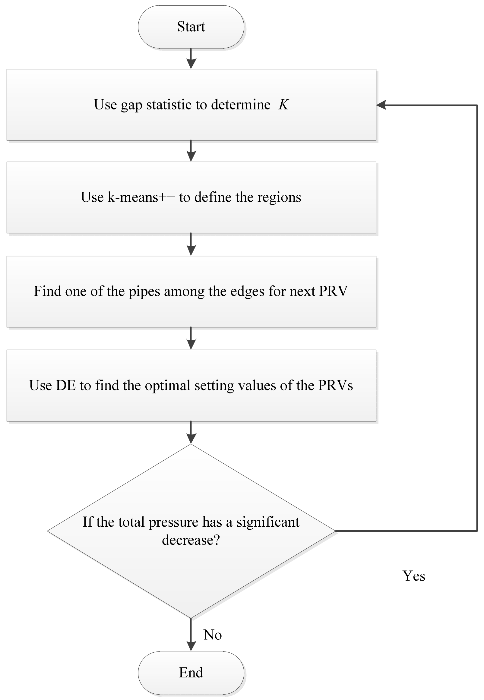
Figure 3 illustrates the software implementation of the proposed method. For a given WDS, we use the EPANET [41] model as a simulator to calculate the pressure trajectories at the nodes. the numbers of PSs and PRVs are not required to be specified a priori. The output of the algorithm will provide these numbers and their locations as well as the PRV setting values.
The algorithm is an iterative search approach. In each iteration, the gap statistic method is used at first to determine the number of pressure regions K which is the number of regions of the WDS. Correspondingly, the number of PSs is defined. Then, k-means++ is used to cluster the pressure curves at the nodes into K regions, and then, the centers of these clusters are determined which will be the sensors positions. After that, one pipe among the edges of the regions will be selected to install a new PRV based on the method discussed in Section 3.2. Finally, the setting values of the installed PRVs till now are optimized using the DE method. If the total pressure of the WDS after installing the new PRV is significantly decreased, i.e., there is a potential to further pressure reduction by installing one more PRV, the computation continues to the next iterate. Otherwise, the computation stops and provides the solution.
5. Case Studies
The computation of the case studies was conducted on an Intel (R) Core (TM) 3.20 GHz 8 GB RAM desktop. The total computation time taken for solving the three case study problems was 3.33 h, 3.74 h, and 37.92 h, respectively.
5.1. Case Study 1: Jilin Network
The Jilin network is a hypothetical network first introduced by Bi and Dandy (Figure 4) [42]. The system has 27 nodes and 34 pipes, and one reservoir with a head of 50 (m). The demand pattern involves a 24-hour period change profile. To test our approach, we assume that the lower limit of the pressure at all nodes is 20 (m) to ensure the water supply. Correspondingly, the head of the reservoir is increased to 70 (m).
Table 1 shows the computed results from our approach, indicating the effects when placing the resulting PRVs and PSs. It can be clearly seen from the 2nd column that the total pressure of the network will be reduced if more PRVs are installed. From the 3rd column, we see that the minimum pressure requirement is satisfied. From the 5th column, it can be seen that the number of PSs (or the number of pressure regions) increases, as the number of PRVs increases. This is because a higher number of PRVs leads to a lower homogeneity of the pressure in the network. From the last column of Table 1, it is shown that the resulting AOR is higher than 80% in this example.
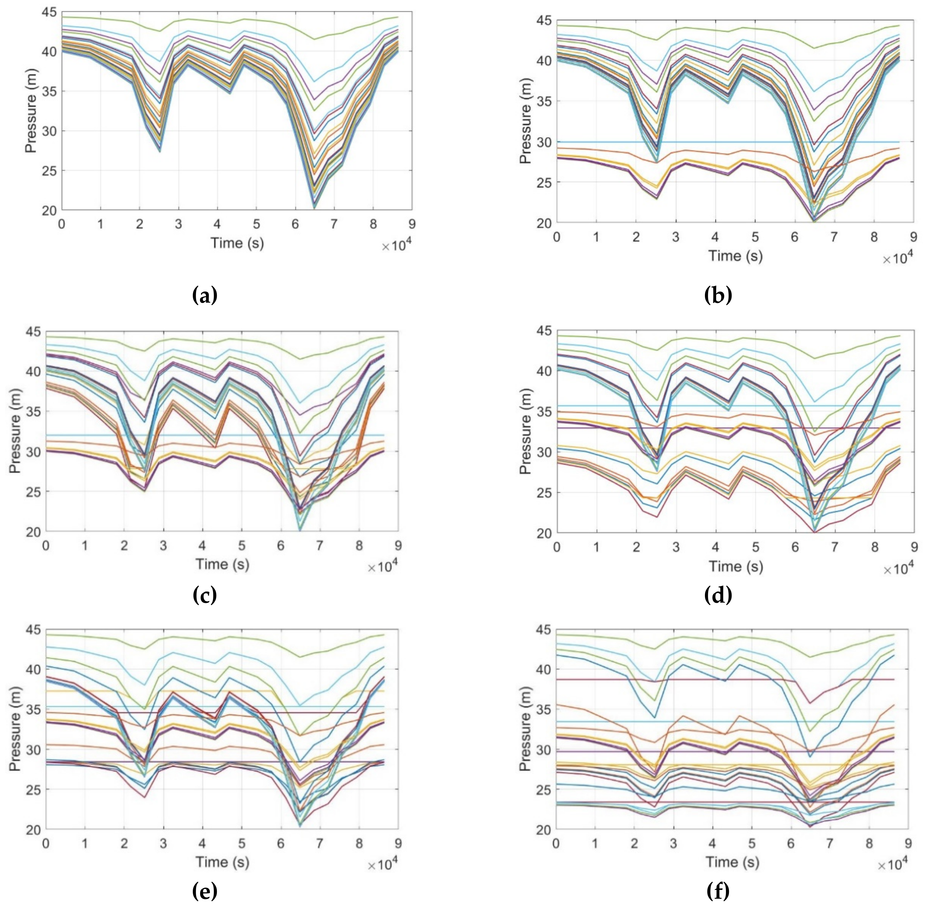
Figure 5 shows the pressure curves of the network corresponding to the results shown in Table 1. It can be seen from Figure 5a–f that there is a clear decrease of the pressures at the nodes, and at the same time, the distribution of the pressure curves is more scattered, as the number of PRVs increases. In addition, 6 PSs are placed in the cases of Figure 5a–c, but their corresponding AOR values are decreased, as shown in the last column of Table 1, due to the growth of the number of PRVs. It means that, although the same number of sensors is used in these three cases, their degree of representation is different. However, when comparing Figure 5d,e, it is seen that the pressure curves with 3 PRVs (Figure 5d) scatter more heavily than those with 4 PRVs (Figure 5e), confirming the AOR values (80.67% and 84.35% both with 7 PSs, respectively) as shown in Table 1. However, this result is illogical based on our discussion in Section 3. The reason may be due to the fact that the network is quite simple and thus, in some situations, the impact of the number of PRVs on the pressure curves is not reasonably regular.
5.2. Case Study 2: A Benchmark WDS
The layout of this case study is shown in Figure 6. The data of the network can be found in [43,44]. The heads at reservoir nodes 23, 24, and 25 (see Figure 6) are set at 54.66 (m), 54.60 (m), and 54.55 (m), respectively. The minimum pressure required at all nodes in the WDS is 30.0 (m).
Similar to the studies in [25,43,44,45], the proposed approach is demonstrated for two cases. In the first case [25], three demand patterns are considered with three multipliers as 0.6, 1.0, and 1.4, respectively. It means that the pressures at the nodes in the network are time-independent, and thus, the sensor placement has no sense in this case. Therefore, in this case, the location of PRVs should be on the link with the maximum pressure drop inside the network.
The results from our approach for the PRV location are given in Table 2 and Table 3. In Table 2, the positions determined from our method are compared with those from [26]. It can be seen that the positions from our results are quite close to those given in [25,26]. However, in Table 3, we only show the total pressure results from our approach, as we do not have the data of the valve settings from [25,26].
In the second case, a 24-hour time-dependent demand pattern is considered, as in [24,26]. Table 4 and Table 5 summarize the computation results. Again, it can be seen from Table 4 that the locations of the PRVs have a slight difference from those given in [24,26]. From Table 5, it is seen that the total pressure will be decreased as the number of PRVs increases, but the reduction will be insignificant when installing 5 to 6 PRVs in the WDS. In addition, the more PRVs we install into the WDS, the worse the AOR of the sensor system will be, as seen in Table 5. This confirms our comment in Section 3 that the PRV placement will have a negative effect on the AOR value of the sensor system.
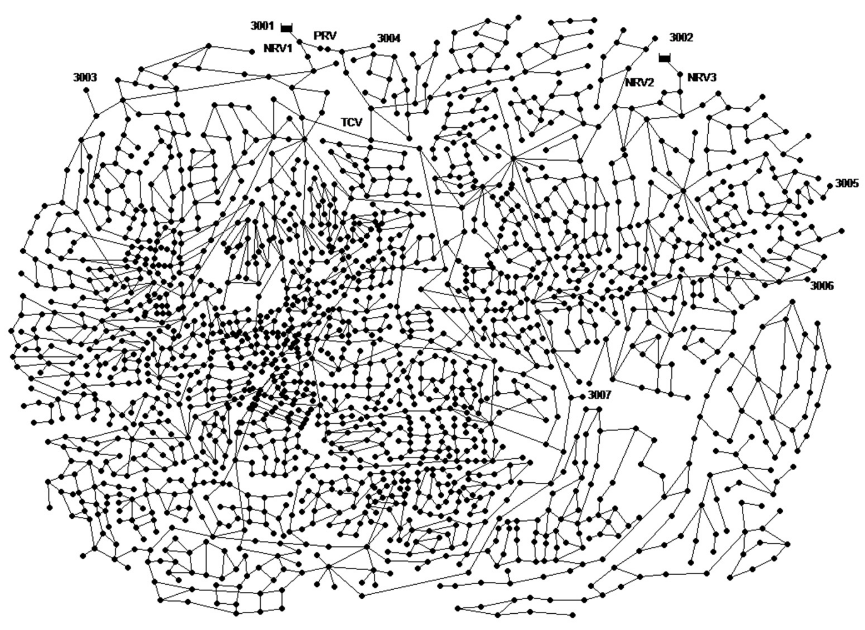
5.3. Case Study 3: Sensor and PRV Localization for EXNET
To investigate the applicability of our approach to a large-scale WDS, an EXNET water distribution network [46] comprising of 2463 links, 1890 nodes, and 2 reservoirs, as shown in Figure 7, is studied. It should be noted that the original system already contains a PRV and a throttle control valve (TCV). The minimal pressure required at all nodes is set to 8 (m) as in [46]. In this study, the head of the two reservoirs is increased to 133.09 (m) and 89.80 (m), respectively.
Table 6 gives our computation results about PRV locations and the total pressure for 24 hours. It is clearly shown that, when installing the PRVs, both the total pressure and the minimum pressure in the network will be significantly reduced. It should be noted that, from our computation results (not shown), some of the PRVs are totally closed in some time periods. This makes sense, because in this large network the first installed PRVs are very close to the reservoirs with a high water head. Thus, they will be closed in some situations for reducing the excess pressure as much as possible.
Figure 8 shows the PS placement and the resulting AOR values of the sensor system, when 8 PRVs are installed in EXNET. The outcome of the gap statistic shows that 11 sensors should be used. It can be seen from Figure 8 that the increase of the AOR value for more than 11 PSs will be insignificant.
In addition, pipe bursts can occur in some pipes in the network. To evaluate the effect of a pipe burst on the values of AOR, we simulate the situation by adding an extra constant demand at some nodes in the WDS, with the installed PRVs and PSs. The position of such a node is randomly selected. It can be seen from Table 7 that the AOR remains almost unaffected. This means that the sensors installed can satisfactorily represent the pressure changes, even if a pipe burst occurs.
6. Conclusions
Due to varying operating conditions, it is necessary to design a closed-loop control system to keep a low pressure of a WDS in real-time. The first task for the control system design is to locate PSs and PRVs in the water network, which remains an open challenge. This study proposes a method that is able to simultaneously determine both the numbers and positions of PSs as well as PRVs. An improved gap statistics algorithm is presented in order to determine the number of sensors and the k-means++ algorithm is used to identify the pressure regions and the sensor locations. A criterion, the accuracy of representation (AOR), is introduced to evaluate the monitoring accuracy of the sensor system. Then, a method for localizing PRVs is proposed based on the sensor positions and the edges of regions. Finally, the setting values of the PRVs are optimized by the differential evolution method. The results of the three case studies illustrate the usability of the proposed approach. Comparisons were made to the available research literature case study data on PRV’s locations. Further tests for exploring the entire method capabilities are warranted for additional and more complex case studies. In addition, based on the determined positions of the PSs and PRVs, our next study will be on the controller design to realize a closed-loop control for WDSs. This will be challenging, as a multi-input/multi-output control system has to be considered.
Author Contributions
Conceptualization, P.L. and A.O.; Methodology, H.C.; Software, H.C.; Validation, H.C., S.H. and E.S.; Formal Analysis, P.L.; Investigation, H.C.; Resources, S.H. and E.S.; Data Curation, H.C..; Writing—Original Draft Preparation, H.C.; Writing—Review & Editing, P.L. and A.O.; Visualization, H.C.; Supervision, P.L. and S.H.; Project Administration, P.L. and A.O.; Funding Acquisition, H.C. and E.S.
Funding
The APC was funded by the German Research Foundation (DFG) with grant LI 806/20-1 and the Open Access Publication Fund of the Technische Universität Ilmenau.
Acknowledgments
We thank Pham Duc Dai for the data from his previous work. We also thank the reviewers for their helpful suggestions for improving the quality of our paper.
Conflicts of Interest
The authors declare no conflict of interest.
References
- Lambert, A.O. International report: Water losses management and techniques. Water Sci. Technol. Water Supply 2002, 2, 1–20. [Google Scholar] [CrossRef]
- Savic, D.A.; Walters, G.A. Integration of a model for hydraulic analysis of water distribution networks with an evolution program for pressure regulation. Comput. Aided Civ. Infrastruct. Eng. 1996, 11, 87–97. [Google Scholar] [CrossRef]
- Vicente, D.J.; Garrote, L.; Sanchez, R.; Santillan, D. Pressure management in water distribution systems: Current status, proposals, and future trends. J. Water Resour. Plan. Manag. 2016, 142, 04015061. [Google Scholar] [CrossRef]
- Ulanicki, B.; Bounds, P.L.M.; Rance, J.P.; Reynolds, L. Open and closed loop pressure control for leakage reduction. Urban Water 2000, 2, 105–114. [Google Scholar] [CrossRef]
- Fontana, N.; Giugni, M.; Glielmo, L.; Marini, G.; Zollo, R. Real-time control of pressure for leakage reduction in water distribution network: Field experiments. J. Water Resour. Plan. Manag. 2018, 144. [Google Scholar] [CrossRef]
- Wang, Y.; Puig, V.; Cembrano, G. Non-linear economic model predictive control of water distribution networks. J. Process Control 2017, 56, 23–34. [Google Scholar] [CrossRef] [Green Version]
- Sun, C.; Morley, M.; Savic, D.; Puig, V.; Cembrano, G.; Zhang, Z. Combining model predictive control with constraint-satisfaction formulation for the operative pumping control in water networks. Procedia Eng. 2015, 119, 963–972. [Google Scholar] [CrossRef]
- Baunsgaard, K.M.H.; Ravn, O.; Kallesøe, C.S.; Poulsen, N.K. MPC control of water supply networks. In Proceedings of the 2016 European Control Conference (ECC), Aalborg, Denmark, 29 June–1 July 2016; pp. 1770–1775. [Google Scholar]
- Renaud, E.; Sissoko, M.T.; Clauzier, M.; Gilbert, D.; Sandraz, A.C.; Pillot, J. Comparative study of different methods to assess average pressures in water distribution zones. Water Util. J. 2015, 10, 25–35. [Google Scholar]
- Halkijevic, I.; Vouk, D.; Posavcic, H. Average pressure in a water supply system. In Proceedings of the 15th International Symposium on Water Management and Hydraulic Engineering, Primošten, Croatia, 6–8 September 2017; pp. 1–11. [Google Scholar]
- Isovitsch, S.L.; VanBriesen, J.M. Sensor placement and optimization criteria dependencies in a water distribution system. J. Water Resour. Plan. Manag. 2008, 134, 186–196. [Google Scholar] [CrossRef]
- Krause, A.; Leskovec, J.; Guestrin, C.; VanBriesen, J.; Faloutsos, C. Efficient sensor placement optimization for securing large water distribution networks. J. Water Resour. Plan. Manag. 2008, 134, 516–526. [Google Scholar] [CrossRef]
- Aral, M.M.; Guan, J.; Maslia, M.L. Optimal design of sensor placement in water distribution networks. J. Water Resour. Plan. Manag. 2010, 136, 5–18. [Google Scholar] [CrossRef]
- Casillas, M.V.; Puig, V.; Garza-Castañón, L.E.; Rosich, A. Optimal sensor placement for leak location in water distribution networks using genetic algorithms. Sensors 2013, 13, 14984–15005. [Google Scholar] [CrossRef] [PubMed]
- Perez, R.; Sanz, G.; Puig, V.; Quevedo, J.; Escofet, M.A.C.; Nejjari, F.; Meseguer, J.; Cembrano, G.; Tur, J.M.M.; Sarrate, R. Leak localization in water networks: A model-based methodology using pressure sensors applied to a real network in Barcelona [applications of control]. IEEE Control Syst. Mag. 2014, 34, 24–36. [Google Scholar]
- Yoo, D.G.; Chang, D.E.; Song, Y.H.; Lee, J.H. Optimal placement of pressure gauges for water distribution networks using entropy theory based on pressure dependent hydraulic simulation. Entropy 2018, 20, 576. [Google Scholar] [CrossRef]
- Steffelbauer, D.; Neumayer, M.; Günther, M.; Fuchs-Hanusch, D. Sensor placement and leakage localization considering demand uncertainties. Procedia Eng. 2014, 89, 1160–1167. [Google Scholar] [CrossRef]
- Christodoulou, S.E.; Gagatsis, A.; Xanthos, S.; Kranioti, S.; Agathokleous, A.; Fragiadakis, M. Entropy-based sensor placement optimization for waterloss detection in water distribution networks. Water Resour. Manag. 2013, 27, 4443–4468. [Google Scholar] [CrossRef]
- Soldevila, A.; Blesa, J.; Tornil-Sin, S.; Fernandez-Canti, R.M.; Puig, V. Sensor placement for classifier-based leak localization in water distribution networks using hybrid feature selection. Comput. Chem. Eng. 2017, 108, 152–162. [Google Scholar] [CrossRef]
- Covelli, C.; Cimorelli, L.; Cozzolino, L.; Morte, R.D.; Pianese, D. Reduction in water losses in water distribution systems using pressure reduction valves. Water Supply 2016, 16, 1033–1045. [Google Scholar] [CrossRef] [Green Version]
- Creaco, E.; Alvisi, S.; Franchini, M. Multistep approach for optimizing design and operation of the C-Town pipe network model. J. Water Resour. Plan. Manag. 2016, 142, C4015005. [Google Scholar] [CrossRef]
- Prescott, S.L.; Ulanicki, B. Improved control of pressure reducing valves in water distribution networks. J. Hydraul. Eng. 2008, 134, 56–65. [Google Scholar] [CrossRef]
- Hindi, K.S.; Hamam, Y.M. Locating pressure control elements for leakage minimization in water supply networks: An optimization model. Eng. Optim. 1991, 17, 281–291. [Google Scholar] [CrossRef]
- Araujo, L.S.; Ramos, H.; Coelho, S.T. Pressure control for leakage minimisation in water distribution systems management. Water Resour. Manag. 2006, 20, 133–149. [Google Scholar] [CrossRef]
- Nicolini, M.; Zovatto, L. Optimal location and control of pressure reducing valves in water networks. J. Water Resour. Plan. Manag. 2009, 135, 178–187. [Google Scholar] [CrossRef]
- Dai, P.D.; Li, P. Optimal localization of pressure reducing valves in water distribution systems by a reformulation approach. Water Resour. Manag. 2014, 28, 3057–3074. [Google Scholar] [CrossRef]
- Savic, D.A.; Walters, G.A. An evolution program for optimal pressure regulation in water distribution networks. Eng. Optim. 1995, 24, 197–219. [Google Scholar] [CrossRef]
- Dai, P.D.; Li, P. Optimal pressure regulation in water distribution systems based on an extended model for pressure reducing valves. Water Resour. Manag. 2016, 30, 1239–1254. [Google Scholar] [CrossRef]
- Lloyd, S. Least squares quantization in PCM. IEEE Trans. Inf. Theory 1982, 28, 129–137. [Google Scholar] [CrossRef]
- Jain, A.K.; Dubes, R.C. Algorithms for Clustering Data; Prentice-Hall: Englewood Cliffs, NJ, USA, 1988. [Google Scholar]
- Wu, X.; Kumar, V.; Quinlan, J.R.; Ghosh, J.; Yang, Q.; Motoda, H.; McLachlan, G.J.; Ng, A.; Liu, B.; Yu, P.S.; et al. Top 10 algorithms in data mining. Knowl. Inf. Syst. 2008, 14, 1–37. [Google Scholar] [CrossRef]
- Arthur, D.; Vassilvitskii, S. k-Means++: The advantages of careful seeding. In Proceedings of the Eighteenth Annual ACM-SIAM Symposium on Discrete Algorithms, New Orleans, LA, USA, 7–9 January 2007; pp. 1027–1035. [Google Scholar]
- Sieranoja, S.; Fränti, P. Random projection for k-means clustering. In Artificial Intelligence and Soft Computing, Proceedings of ICAISC 2018, Zakopane, Poland, 3–7 June 2018; Springer: Berlin/Heidelberg, Germany, 2018; pp. 680–689. [Google Scholar]
- Tibshirani, R.; Walther, G.; Hastie, T. Estimating the number of clusters in a data set via the gap statistic. J. R. Stat. Soc. Ser. B 2001, 63, 411–423. [Google Scholar] [CrossRef]
- Yan, M.; Ye, K. Determining the number of clusters using the weighted gap statistic. Biometrics 2007, 63, 1031–1037. [Google Scholar] [CrossRef]
- Scott, A.J.; Symons, M.J. Clustering methods based on likelihood ratio criteria. Biometrics 1971, 27, 387–397. [Google Scholar] [CrossRef]
- Dunn, J.C. A fuzzy relative of the ISODATA process and its use in detecting compact well-separated clusters. J. Cybern. 1973, 3, 32–57. [Google Scholar] [CrossRef]
- Khezzar, L.; Harous, S.; Benayoune, M. Steady-state analysis of water distribution networks including pressure-reducing valves. Comput. Aided Civ. Infrastruct. Eng. 2001, 16, 259–267. [Google Scholar] [CrossRef]
- Storn, R.; Price, K. Differential evolution—A simple and efficient heuristic for global optimization over continuous spaces. J. Glob. Optim. 1997, 11, 341–359. [Google Scholar] [CrossRef]
- Wang, Y.; Cai, Z.; Zhang, Q. Differential evolution with composite trial vector generation strategies and control parameters. IEEE Trans. Evol. Comput. 2011, 15, 55–66. [Google Scholar] [CrossRef]
- Rossman, L.A. EPANET 2 Users Manual; US Environmental Protection Agency: Washington, WA, USA, 2000.
- Bi, W.; Dandy, G.C. Optimization of water distribution systems using online retrained metamodels. J. Water Resour. Plan. Manag. 2014, 140. [Google Scholar] [CrossRef]
- Sterling, M.J.H.; Bargiela, A. Leakage reduction by optimised control of valves in water networks. Trans. Inst. Meas. Control 1984, 6, 293–298. [Google Scholar] [CrossRef]
- Jowitt, P.W.; Xu, C. Optimal valve control in water-distribution networks. J. Water Resour. Plan. Manag. 1990, 116, 455–472. [Google Scholar] [CrossRef]
- Reis, L.; Porto, R.; Chaudhry, F. Optimal location of control valves in pipe networks by genetic algorithm. J. Water Resour. Plan. Manag. 1997, 123, 317–326. [Google Scholar] [CrossRef]
- Eck, B.; Mevissen, M. Valve Placement in Water Networks: Mixed-Integer Mon-Linear Optimization with Quadratic Pipe Friction; IBM Research Report No. RC25307(IRE1209-014); IBM Research Smarter Cities Technology Centre: Dublin, Ireland, 28 September 2012. [Google Scholar]
Figure 1.
An illustrative example of a WDS with three pressure regions.

Figure 2.
An example of valve placement.

Figure 3.
Algorithm of the proposed approach.

Figure 4.
Jilin Network [42].
Figure 4.
Jilin Network [42].

Figure 5.
The pressure curves of the Jilin Network. (a) The original system; (b) with 1 PRV; (c) with 2 PRVs; (d) with 3 PRVs; (e) with 4 PRVs; (f) with 5 PRVs.
Figure 5.
The pressure curves of the Jilin Network. (a) The original system; (b) with 1 PRV; (c) with 2 PRVs; (d) with 3 PRVs; (e) with 4 PRVs; (f) with 5 PRVs.


Figure 8.
AOR values with different number of sensors.


Table 1.
Total pressure (24 h) with PRVs and AOR with PSs.
| No. of PRVs | Total Pressure (m) | Min. Pressure (m) | Setting Value of PRVs | No. of PSs | AOR |
|---|---|---|---|---|---|
| 0 | 20.1063 | 6 | 93.04% | ||
| 1 | 20.0160 | 29.93 | 6 | 84.46% | |
| 2 | 20.0123 | 32.01; 27.83 | 6 | 82.72% | |
| 3 | 20.0489 | 35.65; 24.3; 32.91 | 7 | 80.67% | |
| 4 | 20.2887 | 35.32; 37.26; 28.43; 34.55 | 7 | 84.35% | |
| 5 | 20.2836 | 33.44; 28.06; 29.70; 38.7; 23.41 | 9 | 81.27% |
Table 2.
Optimal PRV locations for the WDS benchmark with three demand patterns.
| No. of PRVs | Link IDs [Current Study] | Link IDs [26] | Link IDs [25] |
|---|---|---|---|
| 1 | 11 | 11 | 11 |
| 2 | 11,9 | 11,20 | 11,20 |
| 3 | 11,9,20 | 11,20,21 | 11,20,1 |
| 4 | 11,9,20,21 | 11,20,21,1 | 1,11,20,21 |
Table 3.
Total pressure with PRVs for the WDS benchmark with three demand patterns.
| No. of PRVs | Total Pressure (m) |
|---|---|
| 1 | |
| 2 | |
| 3 | |
| 4 |
Table 4.
Optimal PRV locations with 24 demand patterns.
| No. of PRVs | Link IDs [Current Study] | Link IDs [24] | Link IDs [26] |
|---|---|---|---|
| 2 | 11,10 | 1,11 | 1,11 |
| 3 | 11,10,20 | 11,21,29 | 11,20,21 |
| 4 | 11,10,20,21 | 1,8,11,20 | 1,11,20,29 |
| 5 | 11,10,20,21,18 | 1,8,11,21,29 | 1,11,20,21,29 |
| 6 | 11,10,20,21,18,16 | 1,5,11,8,20,21 | 1,11,20,21,29,31 |
Table 5.
Total pressure (24h) with PRVs for the WDS benchmark with 24 demand patterns.
| No. of PRVs | Total Pressure (m) | No. of PSs | AOR |
|---|---|---|---|
| 0 | 11 | 98.07% | |
| 1 | 11 | 81.27% | |
| 2 | 13 | 84.81% | |
| 3 | 11 | 70.36% | |
| 4 | 13 | 66.33% | |
| 5 | 13 | 59.83% | |
| 6 | 9 | 55.27% |
Table 6.
Total pressure (24 h) with PRVs for the EXNET network.
| No. of PRVs | Total Pressure (m) | Min. Pressure (m) | Link IDs |
|---|---|---|---|
| 1 | 3.4560 | 25.2948 | 3026 |
| 2 | 3.4493 | 25.1376 | 3026; 2490 |
| 3 | 2.8942 | 8.0330 | 3026; 2490; 2341 |
| 4 | 2.7625 | 8.0398 | 3026; 2490; 2341; 4908; |
| 5 | 2.7585 | 8.2901 | 3026; 2490; 2341; 4908; 2714; |
| 6 | 2.7404 | 8.1232 | 3026; 2490; 2341; 4908; 2714; 2512; |
| 7 | 2.7431 | 8.2778 | 3026; 2490; 2341; 4908; 2714; 2512; 4854; |
| 8 | 2.7124 | 8.1086 | 3026; 2490; 2341; 4908; 2714; 2512; 4854; 4898 |
Table 7.
AOR with a pipe burst.
| Burst Scene | Without Burst | Place 1 | Place 2 | Place 3 | Place 4 | Place 5 |
|---|---|---|---|---|---|---|
| AOR | 80.63% | 79.89% | 80.51% | 80.49% | 80.49% | 79.94% |
© 2019 by the authors. Licensee MDPI, Basel, Switzerland. This article is an open access article distributed under the terms and conditions of the Creative Commons Attribution (CC BY) license (http://creativecommons.org/licenses/by/4.0/).
Share and Cite
MDPI and ACS Style
Cao, H.; Hopfgarten, S.; Ostfeld, A.; Salomons, E.; Li, P. Simultaneous Sensor Placement and Pressure Reducing Valve Localization for Pressure Control of Water Distribution Systems. Water 2019, 11, 1352. https://doi.org/10.3390/w11071352
AMA Style
Cao H, Hopfgarten S, Ostfeld A, Salomons E, Li P. Simultaneous Sensor Placement and Pressure Reducing Valve Localization for Pressure Control of Water Distribution Systems. Water. 2019; 11(7):1352. https://doi.org/10.3390/w11071352
Chicago/Turabian StyleCao, Hao, Siegbert Hopfgarten, Avi Ostfeld, Elad Salomons, and Pu Li. 2019. "Simultaneous Sensor Placement and Pressure Reducing Valve Localization for Pressure Control of Water Distribution Systems" Water 11, no. 7: 1352. https://doi.org/10.3390/w11071352
Note that from the first issue of 2016, this journal uses article numbers instead of page numbers. See further details here.