MR-WC-MPS: A Multi-Resolution WC-MPS Method for Simulation of Free-Surface Flows

Abstract

A Multi-Resolution Weakly Compressible Moving-Particle Semi-Implicit (MR-WC-MPS) method is presented in this paper for simulation of free-surface flows. To reduce the computational costs, as with the multi-grid schemes used in mesh-based methods, there is also a need in particle methods to efficiently capture the characteristics of different flow regions with different levels of complexity in different spatial resolutions. The proposed MR-WC-MPS method allows the use of particles with different sizes in a computational domain, analogous to multi-resolution grid in grid-based methods. To evaluate the accuracy and efficiency of the proposed method, it is applied to the dam-break and submarine landslide tests. It is shown that the MR-WC-MPS results, while about 15% faster, are in good agreement with the conventional single-resolution MPS results and experimental results. The remarkable ability of the MR-WC-MPS method in providing robust savings in computational time for up to 60% is then shown by applying the method for simulation of extended submarine landslide test.

1. Introduction

It is well known that the complexity of free-surface flows differs significantly depending on the flow region. Specifically, flow in regions close to the free surface is usually more complex than the flow in regions far enough from the free surface. Therefore, having the same spatial simulation resolution across the entire computational domain is not computationally efficient. Alternatively, to increase the computational efficiency while keeping the simulation accuracy at a desired level, multiple discretization resolutions may be used. Besides the efficiency of multi-resolution simulation of fluid flow, it is sometimes necessary to make the Computational Fluid Dynamics (CFD) codes capable of handling the boundaries or external objects in an extremely higher resolution compared to the resolution of fluid flow; for instance, this often happens in simulations of fluid-structure interaction and flow in vegetated channels (e.g., [1]). In these problems, there are restrictions in thickness of the boundaries or external objects such that the thickness might be extremely small compared to the size of the computational domain. Therefore, if the simulation is performed in single resolution, to model the boundaries or external objects in their actual dimensions, extremely fine discretization of the entire spatial domain is necessary. This demands massive use of computational resources, which is often not affordable. By using a multi-resolution technique, the restrictions on the size of the particles representing objects or boundaries could be satisfied while the fluid flow is simulated in a manageable resolution.

The Moving-Particle Semi-Implicit (MPS) method is a mesh-less method proposed by Koshizuka and Oka [2,3,4] for simulation of free-surface flows. In this method, Navier–Stokes equations are solved in a fully Lagrangian form using a fractional step method which consists of splitting each time step in two steps of prediction and correction. The fluid is represented with particles. The motion of each particle is calculated through interactions with neighboring particles by means of a kernel function. Stability of the simulations, efficiency and ease of free-surface tracking using Lagrangian particles, straightforward boundary treatment, ease of coding, and capability to adopt the computations to Graphical Processing Units (GPUs). architectures (e.g., [5]) are among the advantages of using this method in modeling of free-surface flows. The MPS method has gained a lot of interest among numerical modelers in the past two decades and has been successfully applied to a variety of complex free-surface problems such as sediment transport (e.g., [6,7,8]), dam-break (e.g., [9,10]), fluid-structure interaction (e.g., [11]), flow over porous bed (e.g., [12]), liquid sloshing inside a tank (e.g., [13]), breaking waves on slopes (e.g., [14]), submarine landslide (e.g., [7,15,16]), and oil spilling (e.g., [17]). In addition, the MPS method has been applied to a wide range of engineering applications including coastal and ocean engineering (e.g., [8,18,19]), environmental hydraulics (e.g., [6,20,21]), mechanical engineering (e.g., [22]), structural engineering (e.g., [11,23]), chemical engineering (e.g., [24,25]) and bioengineering (e.g., [26,27]).

Despite the success of the MPS method in different applications, the method still has limitations in terms of efficiency and robustness [28]. The original MPS method is fully incompressible, where the pressure is calculated implicitly by solving a Poisson equation of pressure at each time step. This incompressibility modeling is among the most computationally expensive and memory-consuming components of the MPS method. Thus, when many particles are used, the MPS method will suffer from computational issues as well as computer memory issues. To alleviate the computational issues with the original MPS method, the authors in [28,29] proposed a weakly compressible variation of the MPS method. The Weakly Compressible MPS (WC-MPS) method is a simplified form of the MPS method that replaces the incompressibility model in the standard MPS method with a weakly compressible model. This method is explicit and uses an equation of state to calculate the pressure field. The WC-MPS method, compared to the standard MPS method, requires less computer memory and potentially can speed-up the simulations. The WC-MPS method is validated through the simulation of several free-surface problems including flow over spillways [30] and flow over the sills and in trenches [28].

In this paper, a method called MR-WC-MPS method hereafter is proposed for multi-resolution simulation of free-surface flows based on the WC-MPS method. Recently, several research studies have introduced multi-resolution forms for the incompressible MPS method (e.g., [31,32]). In this paper, however, we aim to extend the WC-MPS formulation for a multi-resolution simulation of fluid flow to benefit from the WC-MPS advantages over the MPS advantages also in the multi-resolution settings. To evaluate the accuracy and stability of this multi-resolution form of WC-MPS (MR-WC-MPS), comparative tests are performed against two well-known test cases, namely dam-break and submarine landslide tests. Simulation results are compared with experimental and conventional MPS results. The ability of the proposed method in providing robust computational time savings is also shown by applying the method for extended submarine landslide simulation. The dam-break test has been used extensively in the literature as a bench-mark problem for verifying free-surface flow simulation methods (e.g., [2,33]). Moreover, due to the importance of water waves generated by landslides, researchers have conducted vast empirical (e.g., [34,35]), analytical (e.g., [36]) and numerical (e.g., [37,38]) studies on this phenomenon.

The remainder of this paper is organized as follows. Fundamentals of the MPS method are described in Section 2. Next, the proposed MR-WC-MPS method is introduced in detail in Section 3. Results for simulations of dam-break and landslide-induced water waves using the MR-WC-MPS method are presented in Section 4. Section 5 concludes the paper.

2. Fundamentals of the MPS Method

In this section, the MPS method is introduced in brief. For detailed description of the MPS method see [2,4,17,39].

2.1. Governing Equations

The Navier–Stokes equations are a set of coupled nonlinear partial differential equations that describe how the velocity, density, pressure, and other quantities of a moving fluid are related. For incompressible fluid, and in Lagrangian form of fluid description, the Navier–Stokes equations are expressed as

$$\left\{\begin{array}{c}\frac{1}{\rho }\frac{D\rho }{Dt}+▽.\mathbf{u}=0,\hfill \\ \frac{D\mathbf{u}}{Dt}=-\frac{1}{\rho }△P+\nu {△}^2\mathbf{u}+\mathbf{f},\hfill \end{array}\right.$$

(1)

in which $\rho$ is the fluid density, t is time, $\mathbf{u}$ is the velocity vector, P is pressure, $\nu$ is kinematic viscosity of fluid and $\mathbf{f}$ is the gravity acceleration.

2.2. MPS Interpolations

In the MPS method, the motion of each particle is calculated based on the interactions with neighboring particles covered by a kernel (weight) function. The third-order spiky kernel function [28] is used for the simulations presented in this paper, which is expressed as

$$w\left(r,r_e\right)={\left(1-\frac{r}{r_e}\right)}^3,$$

(2)

in which $w\left(r,r_e\right)$ is a kernel function, r is the distance between two fluid particles, and $r_e$ is the kernel size. The value of this kernel function out of the kernel size $\left(r>r_e\right)$ is zero. As stated in [28], implementation of this kernel function, compared to the other alternatives common in the literature, will improve the stability of the simulations as it avoids particle inter-penetration and improves the momentum conservation [28].

In the MPS method, particle number density is defined as

$${〈n〉}_i=\sum _{j\ne i}w\left(r_{ij},r_e\right)$$

(3)

The subscripts denote a specific particle.

Koshizuka and Oka [2] expressed the particle interaction models for differential operators. The gradient operator is given as

$${〈▽\varphi 〉}_i=\frac{d}{n_0}\sum _{j\ne i}\left[\frac{{\varphi }_j-\widehat{{\varphi }_i}}{r_{ij}^2}\left({\mathbf{r}}_j-{\mathbf{r}}_i\right)w\left(r_{ij},r_e\right)\right]$$

(4)

in which $\varphi$ is an arbitrary scalar, $\widehat{{\varphi }_i}$ s the minimum value of that scalar among the neighboring particles of a reference particle i, d is the number of space dimensions, $\mathbf{r}$ is the position vector, and $n_0$ is the constant particle number density.

The Laplacian operator is modeled in a transient diffusion problem and expressed as

$${〈{▽}^2\varphi 〉}_i=\frac{2d}{n_0}\sum _{j\ne i}\left[\left({\varphi }_j-{\varphi }_i\right)w\left(r_{ij},r_e\right)\right]$$

(5)

with some constant $\lambda$.

2.3. Solution Method

A fractional step method is used in the MPS method which consists of splitting each time step in two steps of prediction and correction [4]. At the prediction step, the viscous and gravitational forces are explicitly calculated without enforcing the incompressibility to the fluid and an intermediate velocity and position is obtained for each particle. At the correction step, the fluid incompressibility is enforced, resulting in the following Poisson equation of pressure

$${〈{▽}^2{P}^{n+1}〉}_i=-\frac{\rho }{d{t}^2}\frac{{〈n^{*}〉}_i-n_0}{n_0}$$

(6)

in which $n^{*}$ is the particle number density at the prediction step. This Poisson equation of pressure can be turned to a system of linear equations by replacing the left side of the equation by the Laplacian model expressed in equation. Once the system is solved and the pressure is calculated, it is replaced into the gradient model (Equation (4)) to calculate the pressure gradient. The velocity correction is then calculated using the pressure gradient.

2.4. Weakly Compressible Model

Shakibaeinia and Jin [28] adjusted the equation of state given by Monaghan [40] to be used in the MPS formulation. This equation of state has the form of

$$P_i=\frac{{\rho }_0{C}^2}{\gamma }\left[{\left(\frac{{〈n^{*}〉}_i}{n_0}\right)}^{\gamma }-1\right]$$

(7)

with $\gamma =7$. C is the numerical sound speed. To keep the fluid density variation less than 1% of the reference density, the Mach number (Ma) should be smaller than 0.1. In other words, the numerical sound speed should be ten times higher than the maximum fluid particle velocity. Using this equation of state, the pressure can be obtained explicitly without solving the Poisson equation of pressure. This explicit method is known as Weakly Compressible MPS (WC-MPS) method.

2.5. Boundary Treatment

In the MPS method, a fluid particle is considered on the free surface if it satisfies the following condition

$${〈n^{*}〉}_i<\beta n^0.$$

(8)

Parameter $\beta$ is called the free-surface parameter. The reference pressure is applied to free-surface particles as a boundary condition. Close to solid boundaries, the particle number density of particles will decrease and accordingly, they may satisfy the free-surface boundary condition and be considered on the free-surface. To avoid this issue, a few layers of so-called “ghost particles” are simulated outside the solid boundaries to take part in particle number density calculations. The first layer of solid boundaries will take part in pressure calculations. As a result, there is always a repulsive force between fluid particles and solid boundary particles to avoid sticking of fluid particles to the solid boundaries.

3. Multi-Resolution MPS Method

In this section, the particle interaction mechanism in a multi-resolution representation of computational domain is illustrated. For simplicity and with no loss of generality, we choose to illustrate the mechanism in a two-scale computational domain consisting of two regions represented in two different resolutions. The subsequent generalization to multiple resolutions will be straightforward.

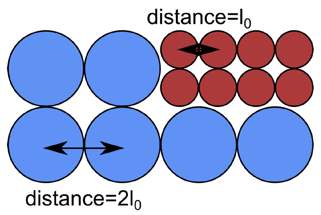
In a computational domain represented in two different resolutions, the low-resolution and high-resolution regions are called, respectively, coarse and fine regions hereinafter. Particles representing the coarse and fine regions are referred to as large and small particles, respectively. The initial particle spacing for large and small particles are $\alpha {\ell }_0$ and ${\ell }_0$, respectively. $\alpha$ is therefore defined as the ratio of large particles spacing to small particles spacing. The initial particle spacing between a pair of a small and a large neighboring particles is consequently $\frac{\alpha +1}{2}{\ell }_0$. Figure 1 shows a sample particle configuration in a two-resolution domain. In this configuration, $\alpha$ is set to 2.

3.1. Calculation of Kernel Function

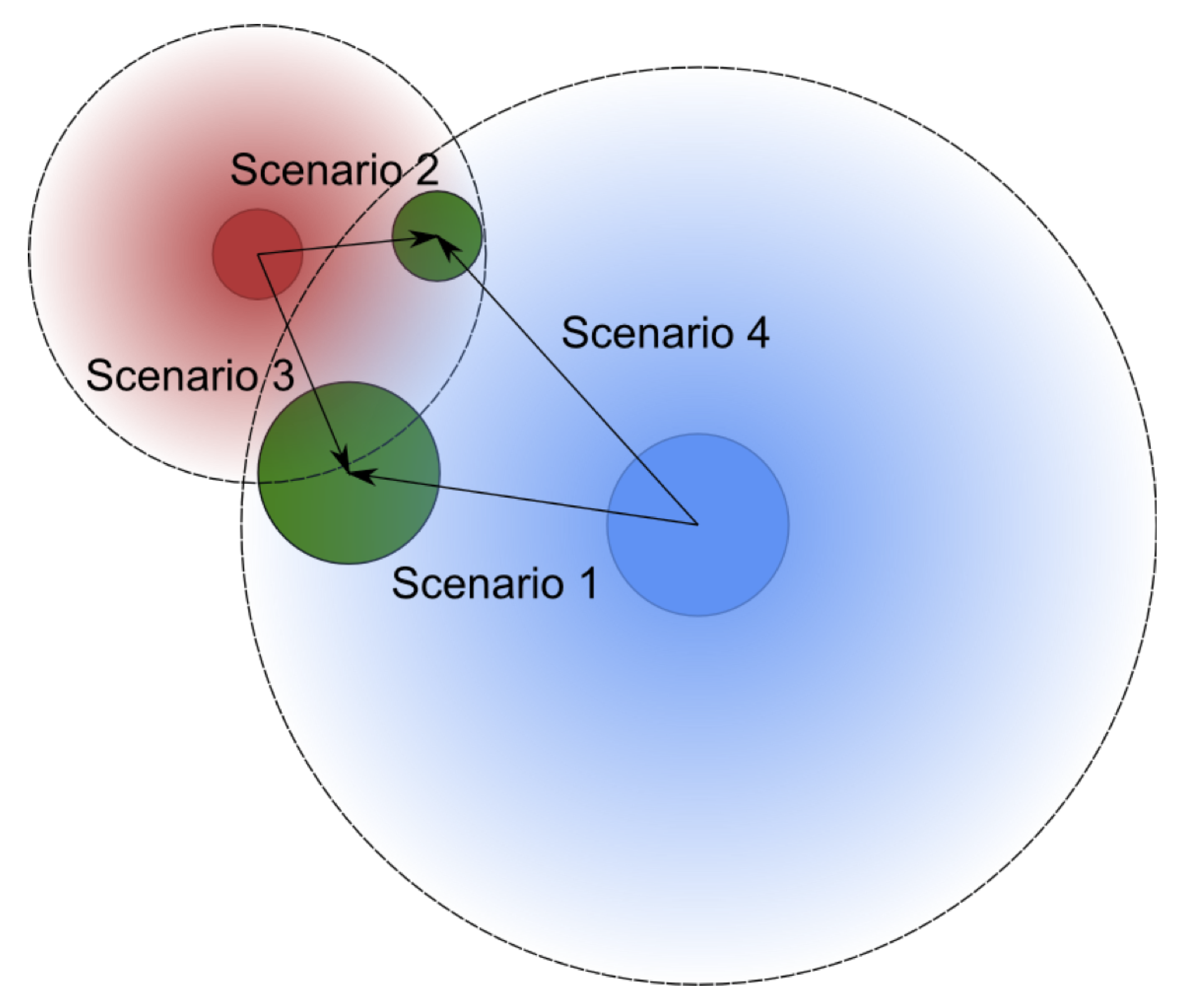
Figure 2 describes the four possible scenarios of particle interaction in a two-resolution computational domain. Kernel function calculation in scenarios 1 and 2 ($w_1\left(r,r_e\right),w_2\left(r,r_e\right)$) is straightforward as the kernel size is clearly specified. The difficulty arises in calculation of kernel function in absence of a specified kernel size (i.e., scenarios 3 and 4). The solution rests in the splitting of large particles. Precisely, when a small particle interacts with a large particle, the large particle will split into fictitious particles. Therefore, interaction between a large and a small particle is considered possible if and only if there exists at least one fictitious particle within the kernel size of the small particle.

The properties of fictitious particles are determined as follows: (1) Size of these particles is the same as the size of small particles, (2) Fictitious particles do not carry any physical variables; the density, velocity, and pressure of their host is assigned to these particles, (3) Kernel size for the fictitious and small particles are equal, (4) Given the position of the host particle $(x,y)$, position of the fictitious particles is $(x+\alpha {\ell }_0/4,y+\alpha {\ell }_0/4)$, $(x-\alpha {\ell }_0/4,y+\alpha {\ell }_0/4)$, $(x-\alpha {\ell }_0/4,y-\alpha {\ell }_0/4)$, and $(x+\alpha {\ell }_0/4,y-\alpha {\ell }_0/4)$.

The kernel function in scenario 3 is calculated as

$$w_3\left(r,r_e\right)=\sum _{i=1}^{{\alpha }^2}w\left(r_i,r_e\right),$$

(9)

in which r is the distance between the small and large particles, $r_e$ is the kernel size for the small particle, and $r_i$ is the distance between the small and ith fictitious particle.

In scenario 4, two different cases should be considered. The first case is when at a time step, a reference large particle interacts only with neighboring small particles. The kernel function in this case is calculated as

$$w_4^{(1)}\left(r,r_e\right)=\frac{{\sum }_{i=1}^{{\alpha }^2}w\left(r_i,r_e\right)}{{\alpha }^2},$$

(10)

which is an arithmetic mean over the interactions of individual fictitious particles with the neighboring particles. The second case happens when the reference large particle is interacting with both small and large neighboring particles. In this case, the interaction between the reference large particle and the neighboring small particles is modeled similar to the first case (Equation (10)). However, when the reference large particle is interacting with another large particle, both particles will be split into fictitious particles. The kernel function for interaction of two large particles in this case is calculated as

$$w_4^{(2)}\left(r,r_e\right)=\frac{{\sum }_{j=1}^{{\alpha }^2}{\sum }_{i=1}^{{\alpha }^2}w\left(r_{ij},r_e\right)}{{\alpha }^2},$$

(11)

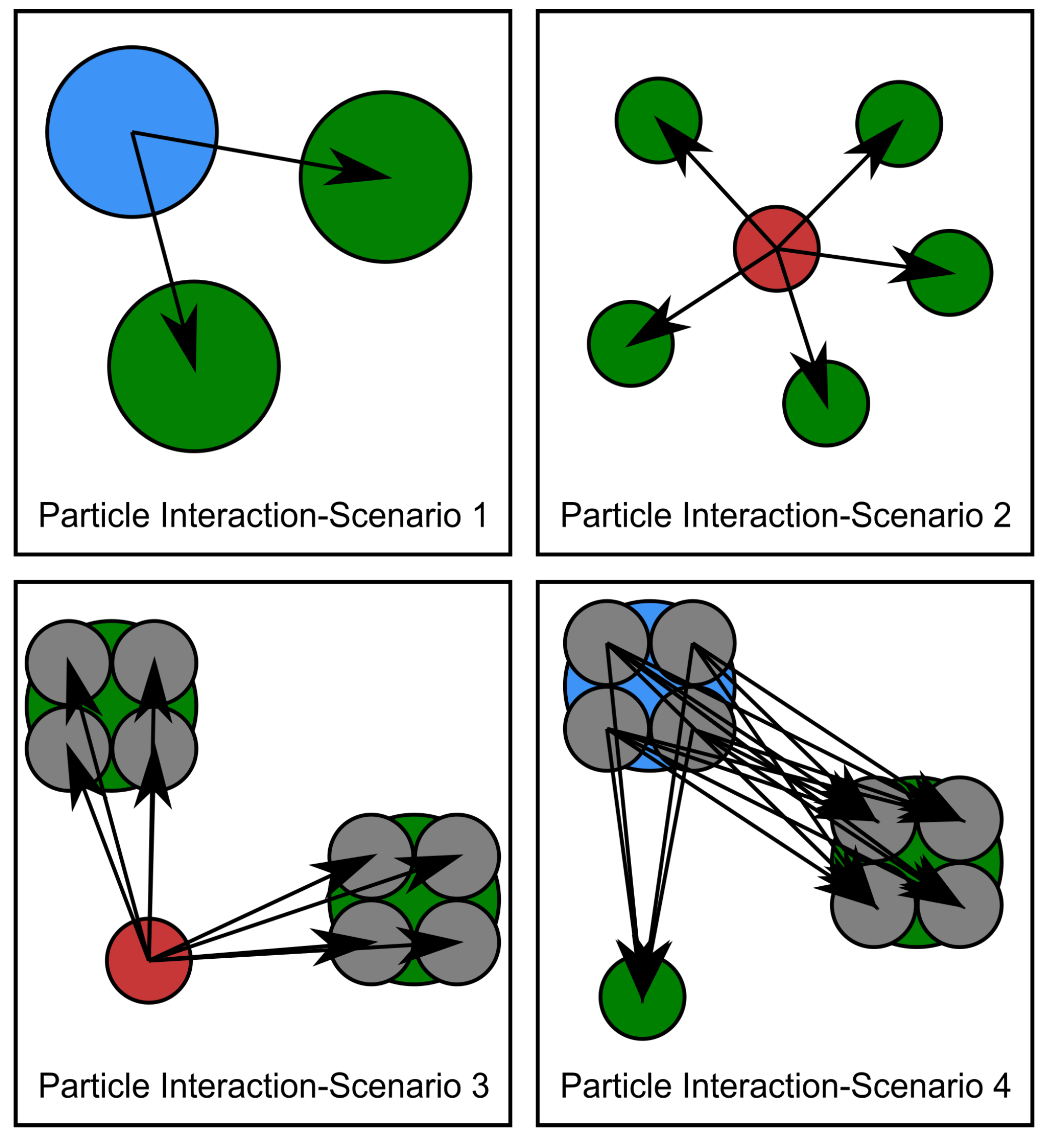
in which $r_{ij}$ is the distance between the fictitious particles i and j, belonging to two different hosts. In this model, both reference and neighboring large particles are being split. Then interaction intensity for individual fictitious particles corresponding to the reference host is calculated. Finally, an arithmetic mean is taken over the interactions of these fictitious particles. Figure 3 depicts a sample particle interaction mechanism in each scenario.

3.2. Calculation of Particle Number Density

When a reference small particle interacts with both neighboring small and large particles at a time step, particle number density is calculated as

$${〈n〉}_i=\sum _{j\ne i}\left[w_2\left(r_{rj},r_e\right)+w_3\left(r_{rj},r_e\right)\right],$$

(12)

the first term on the right-hand side of the equation can be calculated using the interaction model in scenario 2 (standard interaction model in the MPS formulation) and the second term can be calculated using the interaction model introduced in scenario 3.

When a reference large particle interacts only with neighboring large particles at a time step, particle number density is calculated as

$${〈n〉}_i=\sum _{j\ne i}{w}_1\left(r_{rj},r_e\right),$$

(13)

where the right-hand side of the equation can be calculated according to the interaction model introduced in scenario 1, which is the standard interaction model in the MPS formulation. Similarly, when a reference small particle interacts only with neighboring small particles at a time step, particle number density is calculated as

$${〈n〉}_i=\sum _{j\ne i}{w}_2\left(r_{rj},r_e\right),$$

(14)

where the right-hand side of the equation can be calculated according to the interaction model introduced in scenario 2.

When a reference large particle interacts with both neighboring small and large particles at a time step, the particle number density is calculated as

$${〈n〉}_i=\sum _{j\ne i}\left[w_4^{(1)}\left(r_{rj},r_e\right)+w_4^{(2)}\left(r_{rj},r_e\right)\right]+\widehat{w}\left(r,r_e\right),$$

(15)

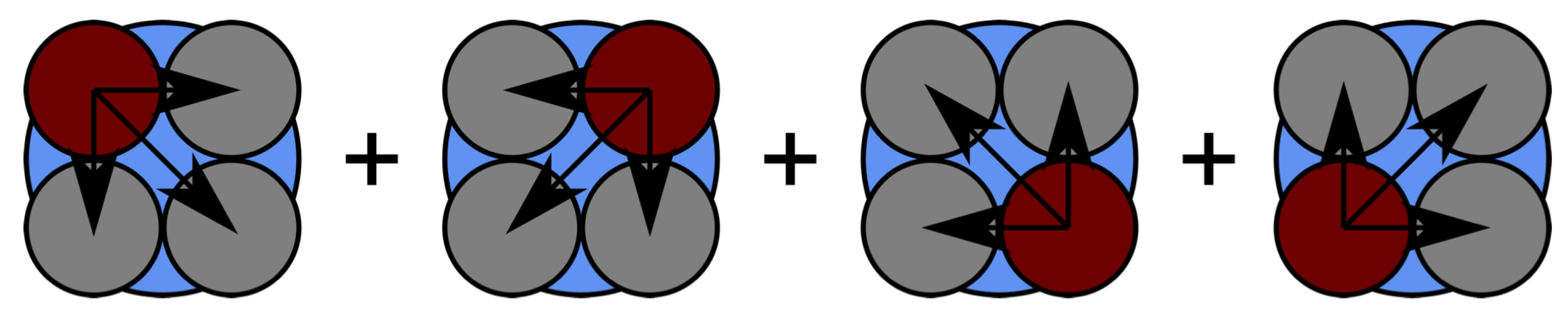
in which both the first and second terms on the right-hand side of the equation can be calculated using the interaction models introduced in scenario 4. The term $\widehat{w}\left(r,r_e\right)$ corresponds to the interaction between the reference fictitious particles with each other. More precisely, when for instance a large particle is being split into four fictitious particles, in order to calculate the particle number density for each of these fictitious particles, in addition to the contribution of the neighboring small and large particles, the contribution of the other fictitious particles corresponding to the host large particle should be also taken into account, as shown in Figure 4. This term is calculated as

$$\widehat{w}\left(r,r_e\right)=\frac{{\sum }_{i=1}^{{\alpha }^2}{\sum }_{j=1,j\ne i}^{{\alpha }^2}{w}_2\left(r_{ij},r_e\right)}{{\alpha }^2}.$$

(16)

3.3. Solution Method

The solution method for the MR-WC-MPS is similar to the MPS with adjustments to the calculation of particle number density, as discussed earlier. The pressure gradient term (Equation (4)) can be calculated in a similar way the particle number density is calculated. Precisely, for a reference particle, each term in the summations (Equations (12)–(15)) is multiplied by another term which is a function of the distance between the reference and a neighboring particle, minimum pressure within the kernel size of the reference particle, and pressure at the location of a neighboring particle. Position of the fictitious particles is calculated according to the position of the reference particle and the initial particle spacing. This will result in big savings in computer memory as opposed to the single-resolution simulation. Size of the time steps should be calculated by the CFL stability condition using the smallest particle spacing in the entire computational domain.

In this algorithm, the constant particle number density $n_0$ remains the same in both fine and coarse regions. Similar to most of the common kernel functions in MPS method, the third-order spiky kernel function used herein (Equation (2)) is a function of one variable (i.e., the ratio of initial particle spacing to kernel size). For all the computational regions (coarse or fine), as the value of this variable is kept the same, the constant particle number density will remain the same.

4. Results and Discussion

4.1. Dam-Break-Induced Water Waves

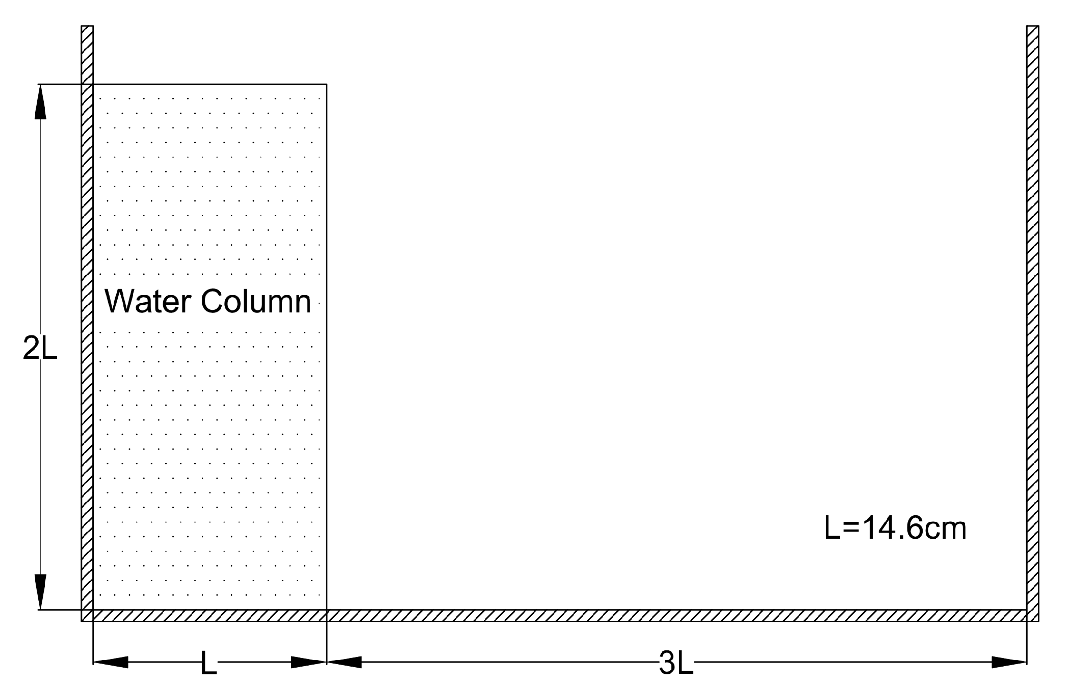
The idealized 2D problem of the instantaneous removal of a barrier holding a water column at rest in a water tank with fixed beds is known as the dam-break problem [2]. This problem has been used as a bench-mark problem for verifying free-surface flow simulation methods [2,33]. In this part, the experimental results for dam-break [2,41] are reproduced numerically using the WC-MPS and the proposed MR-WC-MPS methods. To check the accuracy and efficiency of the proposed MR-WC-MPS method, results are compared with the WC-MPS and standard incompressible MPS methods and the experimental results. Figure 5 shows the dam-break experimental setup.

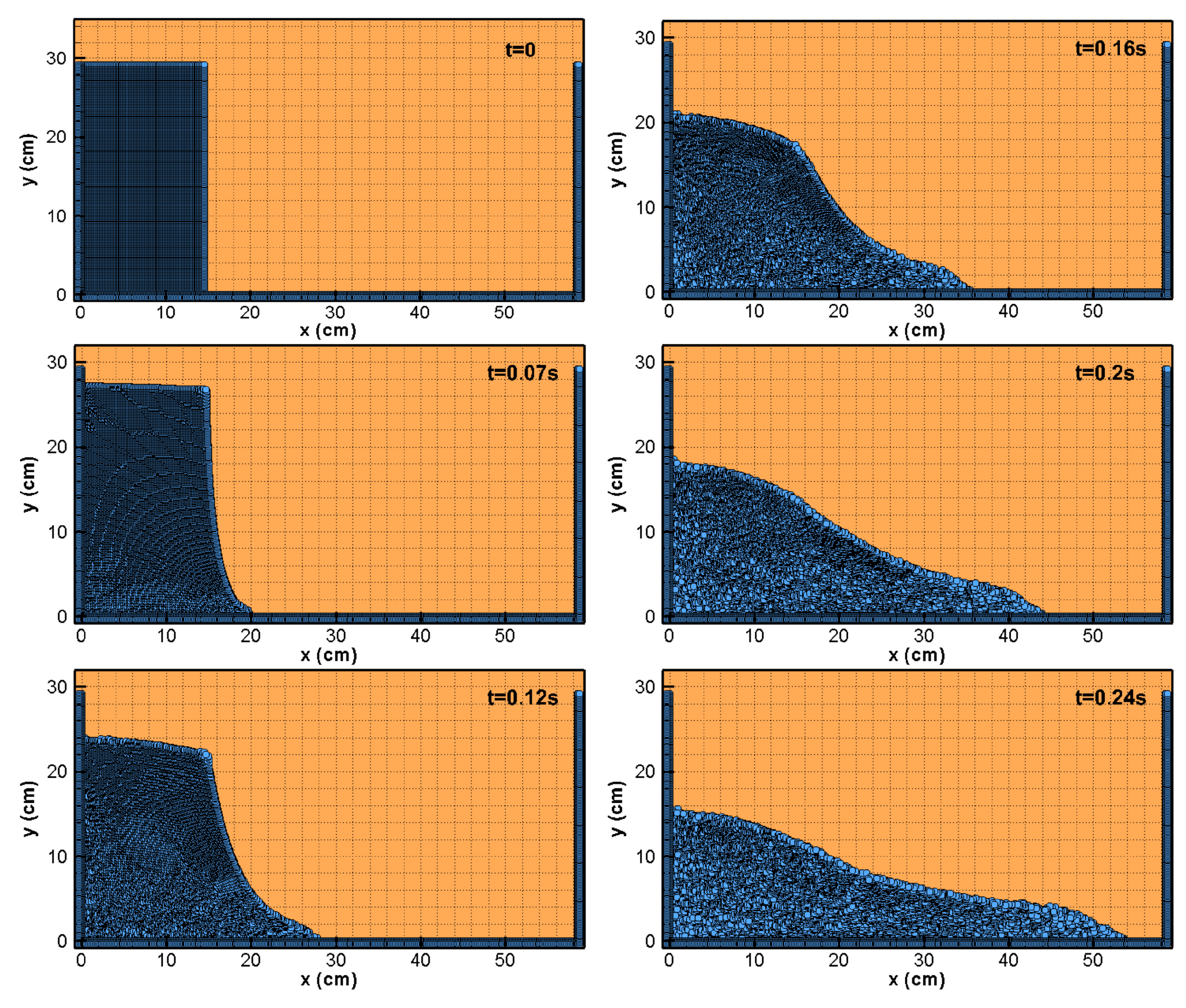
In the present WC-MPS simulation, the initial particle spacing is 0.1825 cm, corresponding to 14,734 particles including fluid, wall, and ghost particles. Free-surface parameter and kernel size are set to 0.99 and 0.365 cm, respectively. The fluid is considered inviscid. The Courant number is set to 0.5. The third-order spiky kernel function (Equation (2)) is used. Two layers of ghost particles are considered. No turbulence modeling is used in this simulation. It is assumed that the barrier holding the water column at rest is removed instantly. Figure 6 shows the computed particle configuration at different times using the WC-MPS method.

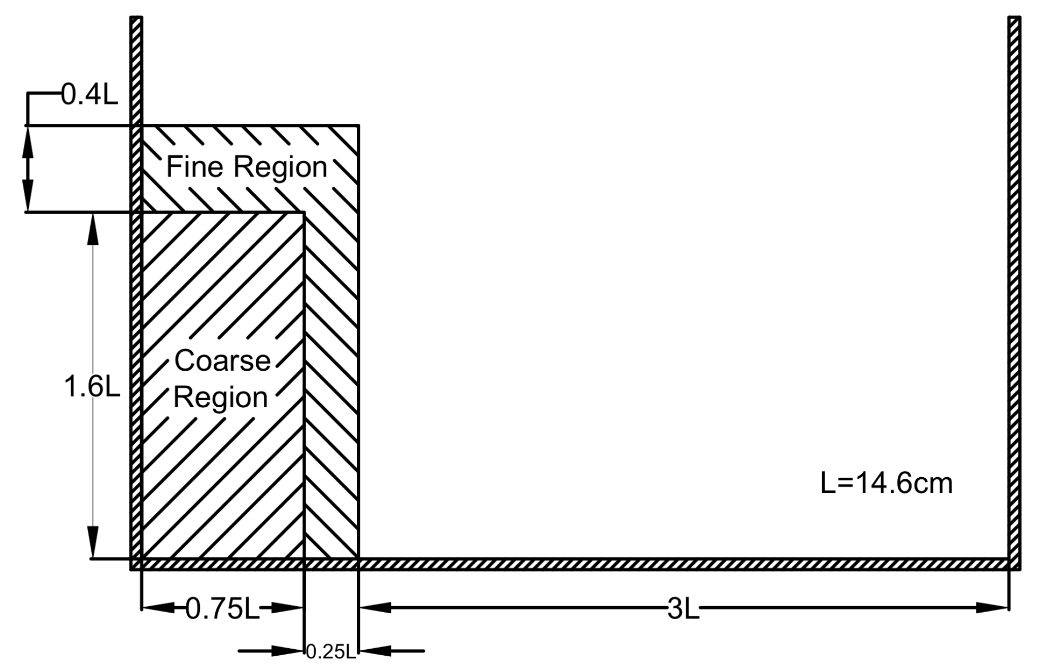
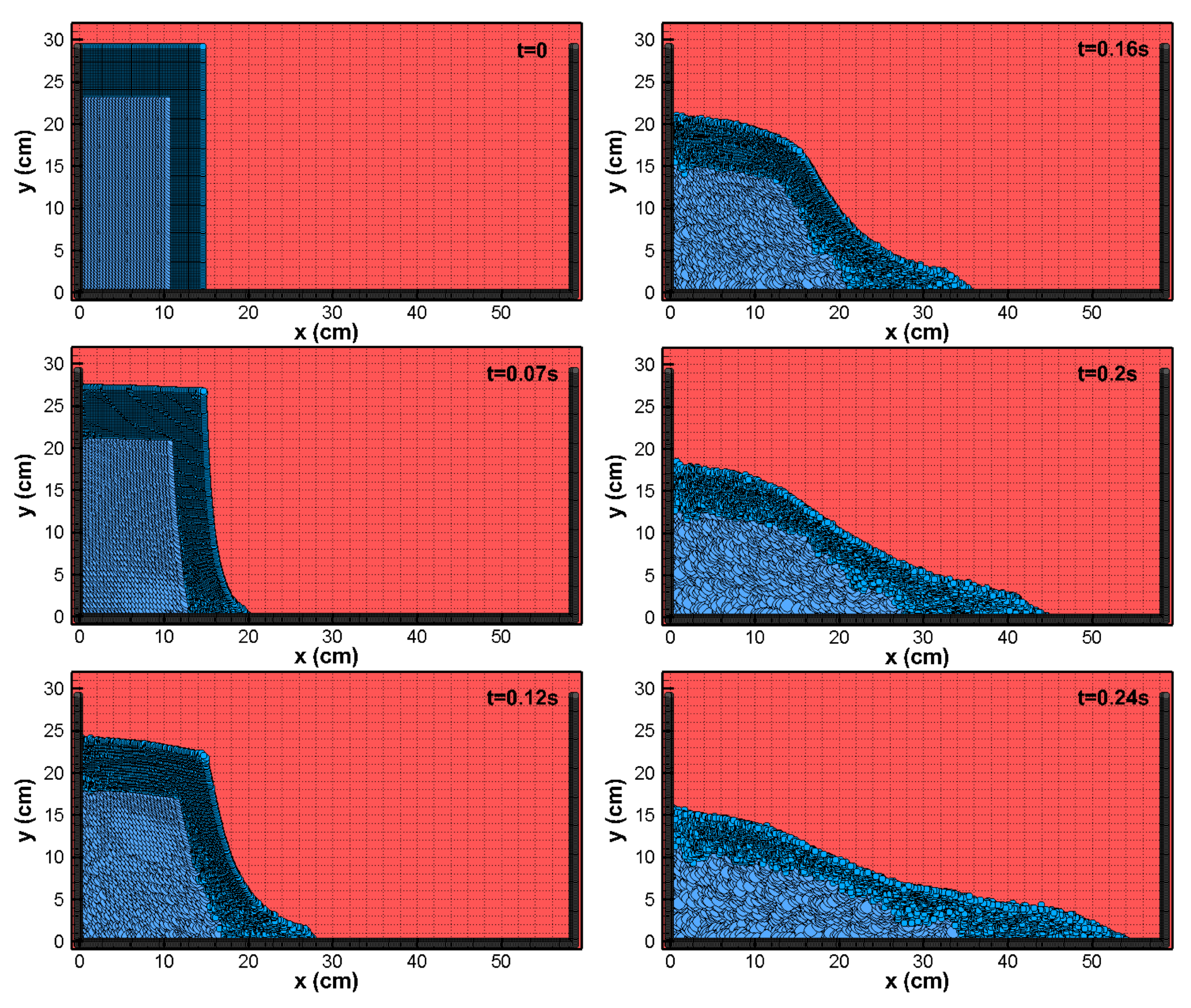
In simulation of the same dam-break problem using the proposed MR-WC-MPS method, calculation parameters are kept similar to those of the WC-MPS simulation. The only difference between the two simulations is that in the MR-WC-MPS simulation, part of the computational domain is represented with large particles with initial particle spacing of 0.365 cm ($\alpha =2$). This reduces the total number of particles to 8975 particles, 40% less than the total number of particles in the WC-MPS simulation. Figure 7 shows the initial setup for the coarse and fine regions in the computational domain. A rectangular region far from the free surface is selected to represent the coarse region. The fluid in this region is expected to have less complex behavior compared to the region with finer resolution. Figure 8 shows the computed particle configuration at different times by the MR-WC-MPS method.

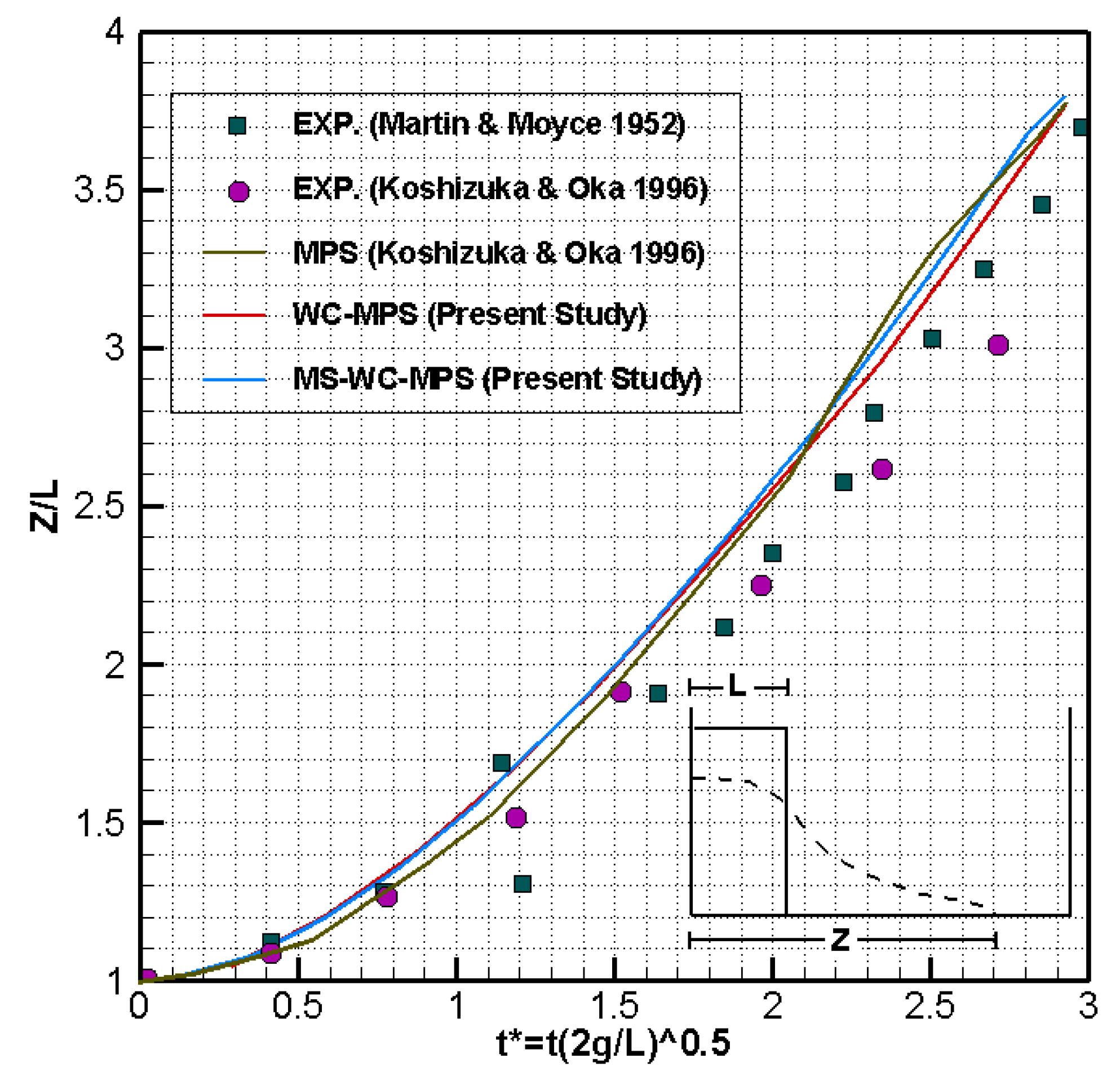
To confirm the accuracy of the proposed MR-WC-MPS method, Figure 9 is depicted. This figure shows a comparison between the experimental, MPS, WC-MPS, and MR- MPS results for the position of dam-break wave front at different times, which has been widely used in the literature for validation purposes (e.g., [2,33,42]). Results of the MPS and WC-MPS simulations are in good agreement with each other and the few discrepancies in the results are due to the use of different compressibility assumptions and calculation parameters. The MR-WC-MPS is in good agreement with both WC-MPS and MPS simulations, showing the accuracy of the proposed method.

The total computational time for the WC-MPS simulation is 373.8 min. The computational time is dropped by about 15% to 321.0 min in the in MR-WC-MPS method. The computer is equipped with Intel^® Core™ i7-2600 3.40 GHz CPU and a system memory of 16.0 GB. Although the calculation of the interactions between large and small particles adds up to the total computational time compared to WC-MPS computational time, the total computational time is reduced.

4.2. Landslide-Induced Water Waves

Landslides, usually caused by slope failures or liquefaction of sediments, can generate water waves and small-scale tsunamis in coastal areas. Once the landslide-induced water waves reach the coast or structures, they can cause disasters including loss of life and collapse of facilities and infrastructures. Therefore, it is of importance to predict the damage of landslide-generated water waves in flood hazard assessment of coastal zones [43].

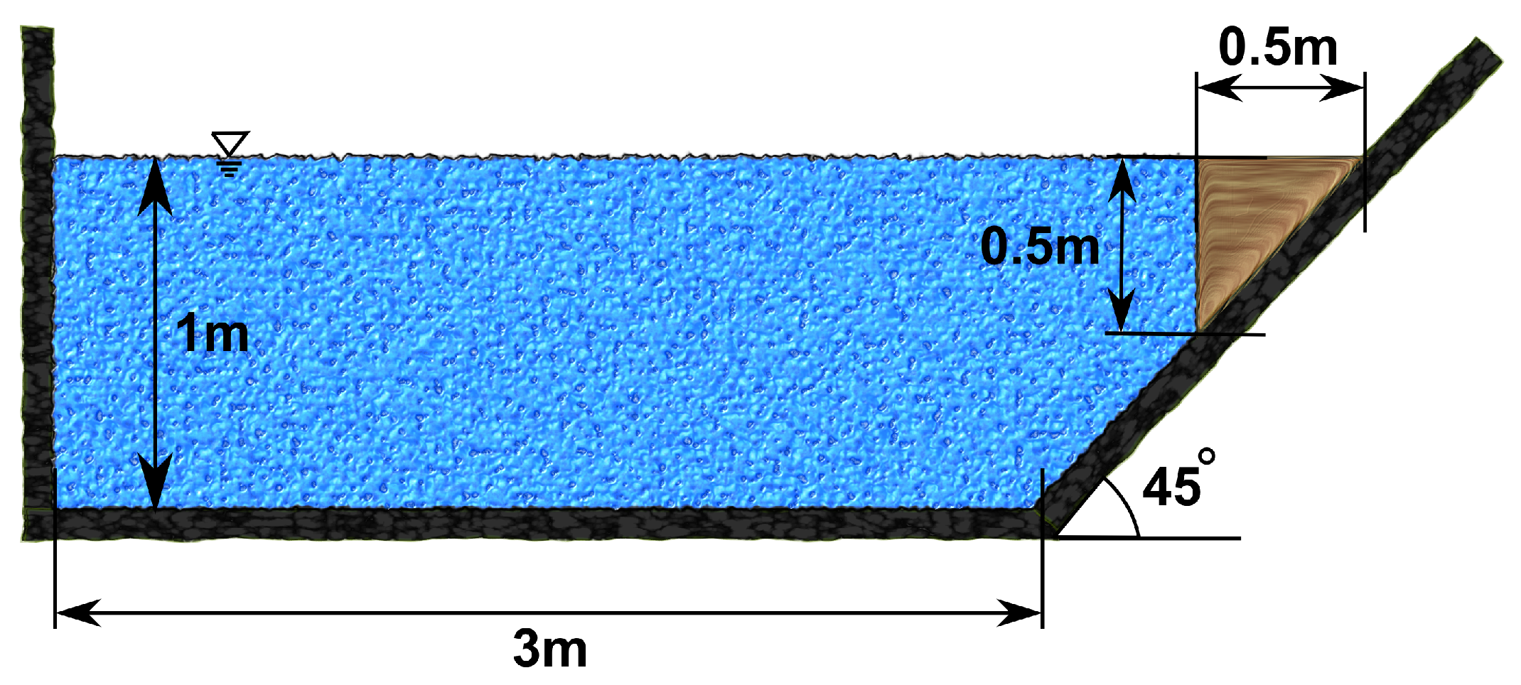
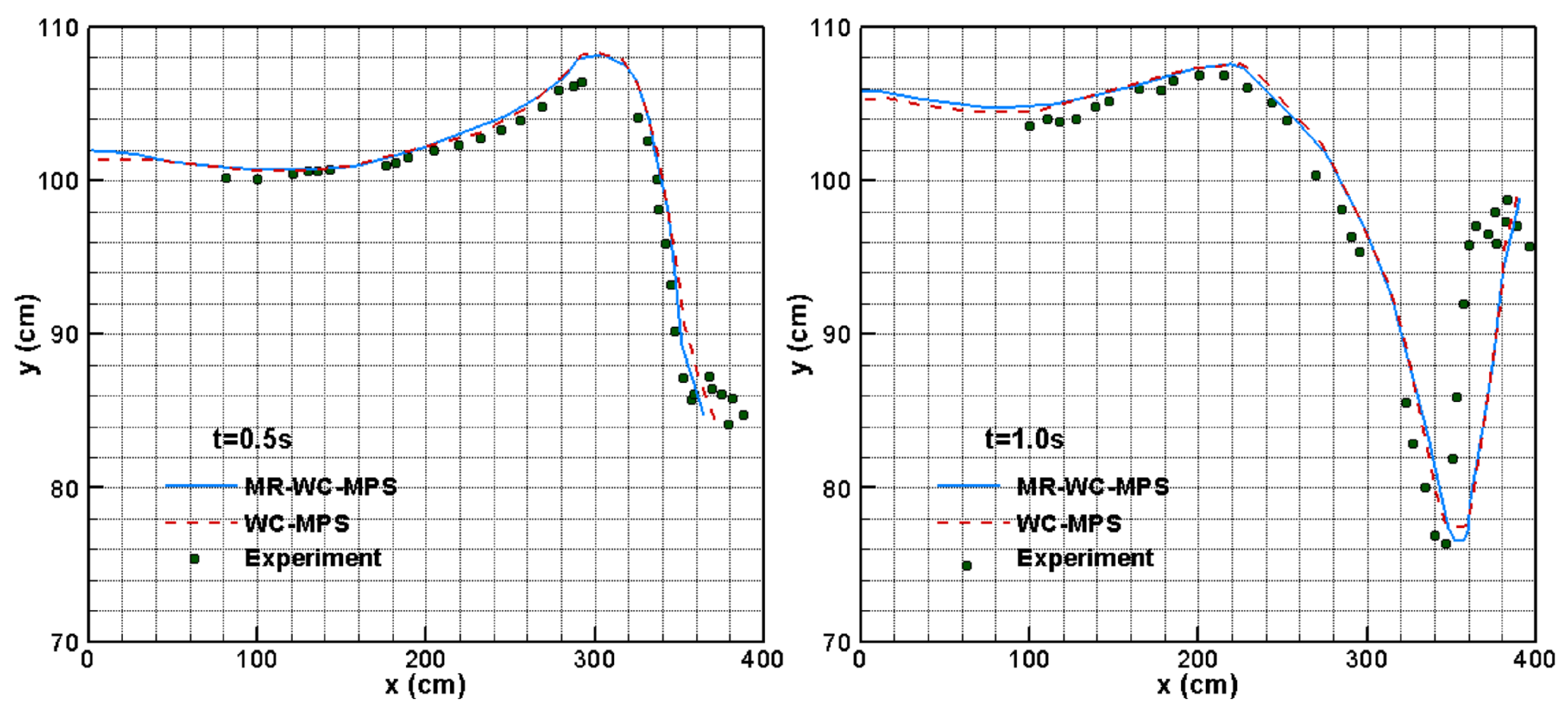
In this part, the experimental results for rigid submarine landslide [44] are reproduced numerically using the WC-MPS and the proposed MR-WC-MPS methods. Results for the free-surface profile are compared with each other to evaluate the accuracy of simulations. Geometry of the problem is shown in Figure 10.

Grilli and Watts [45] have formulated the vertical velocity of the sliding rigid mass in a body of water. During the acceleration phase which lasts for 0.4 s, vertical velocity of the mass is described as

$$V\left(t\right)=c_{1}tanh(c_{2}t),t⩽0.4s,$$

(17)

where $V\left(t\right)$ is the vertical velocity of mass at time t. $c_1$ and $c_2$ are constant values and are set to 86 cm/s and 0.0175 s${}^{-1}$, respectively, following [37]. After the acceleration phase, the vertical velocity of the sliding mass reaches a terminal value of 0.6 m/s. At each time step the velocity of the sliding mass is known; thus, it is straightforward to calculate the position of the sliding mass.

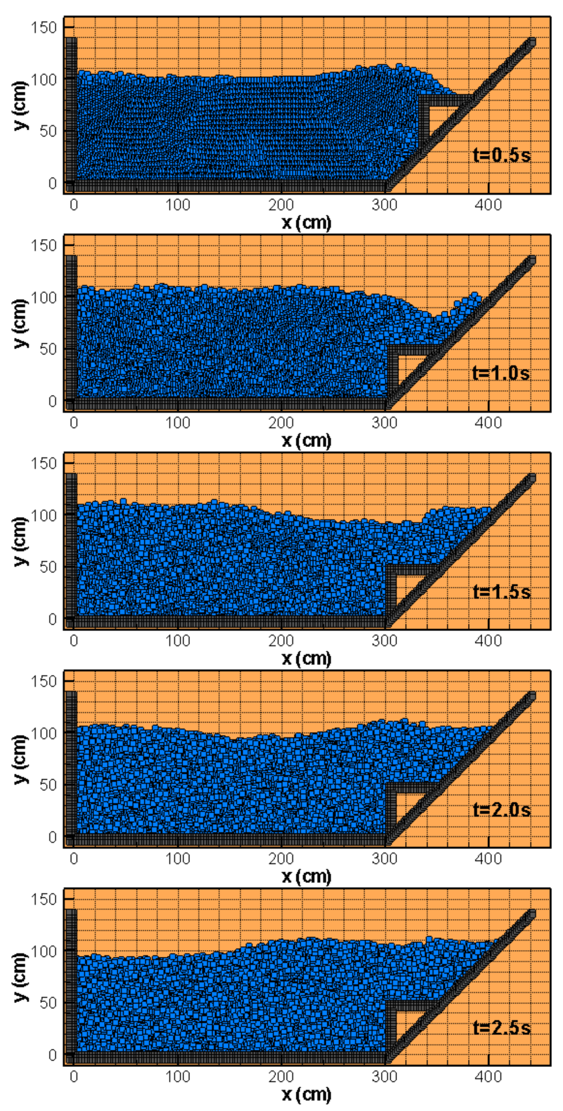
In the present WC-MPS simulation, the third-order spiky kernel function (Equation (2)) is used and the kernel size is set to twice the initial particle spacing. Free-surface parameter is set to 0.99. The fluid is considered inviscid. The solution domain is represented by 6242 particles, in which the initial distance of particles is 2.5 cm. The Courant number is set to 0.5. The numerical value of sound speed is set to 1800 cm/s. Two layers of ghost particles are considered in addition to one layer of solid boundary particles. The simulation is performed for 2.5 s. No turbulence modeling is used in this simulation. Particle configuration at different times is presented in Figure 11. As the mass slides along the inclined wall, the water is heaved up and a wave is formed. At t = 0.6 s, water strikes the right inclined wall. The wave moves toward the left vertical wall and around t = 1.5 s, it reflects from the wall.

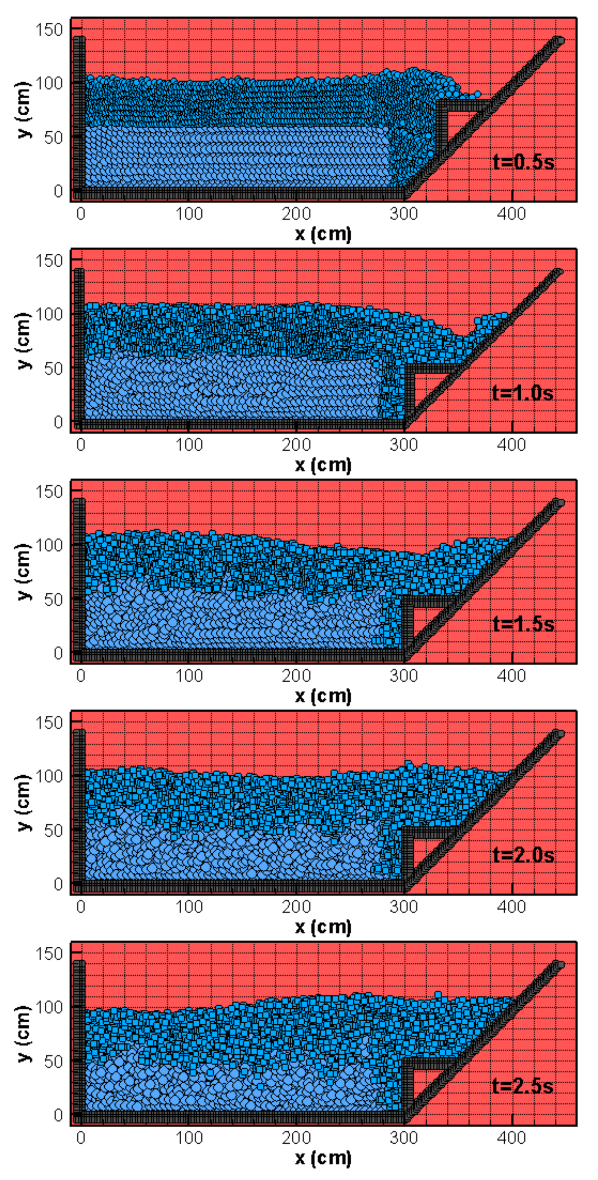
Next, the similar landslide problem is simulated using the proposed MR-WC-MPS method. A 292 cm × 60 cm rectangular region at the bottom left side of the tank is initially discretized with large particles with initial particle spacing of 5 cm ($\alpha =2$). This region will have less complex behavior because the particle initially located in this region will not reach the free surface during the simulation time (2.5 s), as shown in [20], and moreover, these particles will move far enough from the vortex generated by the motion of the submerged mass. Thus, this region may be discretized at a lower resolution to improve the computational efficiency of the simulation. The rest of the computational domain is represented by particles of the same size as of the WC-MPS simulation. The total number of particles representing the computational domain is 4242, which is 68.0% of the total number of particles in the WC-MPS simulation. Other calculation parameters are kept the same as those of the WC-MPS simulation. Figure 12 shows the computed configuration of particles at different times using the proposed MR-WC-MPS method.

The computational time for the WC-MPS simulation is 176.97 min, while it is about 15% less, i.e., 150.33 min, for the MR-WC-MPS simulation. Figure 13 shows a comparison between the WC-MPS, MR-WC-MPS, and experimental results for the water surface profile. It is evident that the discrepancies between the WC-MPS and MR-WC-MPS results are minor. Therefore, by keeping the accuracy at almost the same level, the computational time is decreased.

4.3. Landslide-Induced Water Waves over Extended Tank

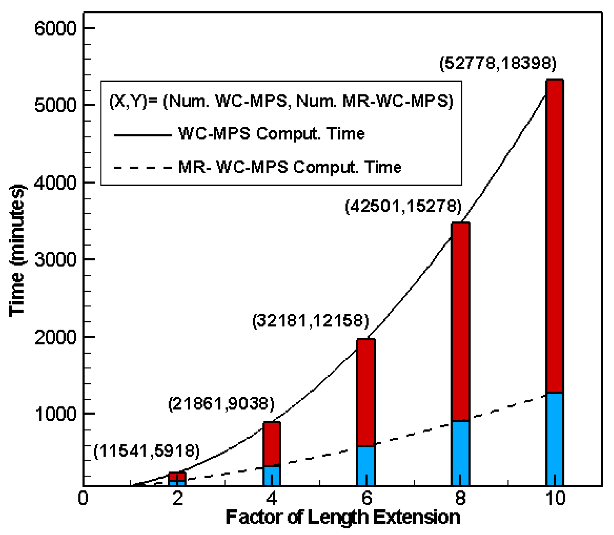
The aim of this part is to show the capability of the proposed MR-WC-MPS method in providing substantial computational time savings when the scale of the simulations is relatively large. To this end, the previous submarine landslide problem is revisited here with a change in the setup; the length of the water tank is extended from the left side by factors of 2, 4, 6, 8, and 10, and in each case, two simulations using the WC-MPS and MR-WC-MPS methods are performed for 1 second and the computational time is recorded.

In the MR-WC-MPS simulations, we set the resolution of the extended region equal to the coarse region resolution in the previous example. Figure 14 shows a comparison between the WC-MPS and MR-WC-MPS computational time. Numbers in the parentheses show the total number of particles used in each WC-MPS and MR-WC-MPS simulations, respectively. The substantial savings in computational time using the proposed technique is evident from this figure. The computational time decreases exponentially with the increase in the factor of length extension. In this example, although a portion of course particles stay near-idle, still it is necessary to model these particles to cope with the geometry of the computational domain. With standard WC-MPS method, the computational domain will be filled with particles of the same size, which can be computationally very expensive, whereas with the proposed MR-WC-MPS method enables us to fill the computational domain partially with coarse particles which can significantly contribute to computational time savings.

5. Conclusions

A new technique, called MR-WC-MPS method, has been introduced for multi-resolution simulation of fluid flow based on the MPS method. As a demonstration, the proposed technique has been shown to improve the computational efficiency of three sample simulations of dam-break, submarine landslide, and extended submarine landslide, with similar levels of accuracy compared to the single-resolution simulations. By performing the submarine landslide test in an extended water tank, it has been shown that the proposed technique offers an accelerated yet accurate way of simulation of fluid flow in medium or large scales.

The proposed method is expected to perform well in problems that involve interaction of fluids with elastic structures, such as flow in vegetated channels, and wind turbine flow simulation. In this type of problems, it is necessary to handle the elastic structures in an extremely higher resolution compared to the average resolution of the fluid flow, as there are sometimes strict restrictions in the thickness of these structures. Therefore, an interesting avenue of research in the future is to evaluate the performance of the MR-WC-MPS method in simulating such multi-phase problems. As another suggestion for future studies, the proposed method can be improved to handle multi-resolution multi-time-scale simulation of free-surface flow, which enables the use of different time-stepping algorithms in different regions of the flow represented in different resolutions. The integration algorithm on the computational domain can be performed in a procedure in which coarse regions are advanced in time, while fine regions are advanced multiple steps to reach the same time as of the coarse regions and the data at different levels are then synchronized.

References

- Larroude, P.; Oudart, T. SPH model to simulate movement of grass meadow of posidonia under waves. Coastal Eng. Proc. 2012, 1, 56. [Google Scholar] [CrossRef]
- Koshizuka, S.; Oka, Y. Moving-particle semi-implicit method for fragmentation of incompressible fluid. Nucl. Sci. Eng. 1996, 123, 421–434. [Google Scholar] [CrossRef]
- Koshizuka, S.; Nobe, A.; Oka, Y. Numerical analysis of breaking waves using the moving particle semi-implicit method. Int. J. Numer. Meth. Fluids 1998, 26, 751–769. [Google Scholar] [CrossRef]
- Koshizuka, S.; Shibata, K.; Kondo, M.; Matsunaga, T. Moving Particle Semi-implicit Method: A Meshfree Particle Method for Fluid Dynamics; Academic Press: Cambridge, MA, USA, 2018. [Google Scholar]
- Hori, C.; Gotoh, H.; Ikari, H.; Khayyer, A. GPU-acceleration for moving particle semi-implicit method. Comput. Fluids 2011, 51, 174–183. [Google Scholar] [CrossRef]
- Nodoushan, E.J.; Shakibaeinia, A. Multiphase mesh-free particle modeling of local sediment scouring with μ (I) rheology. J. Hydroinf. 2019, 21, 279–294. [Google Scholar] [CrossRef]
- Nabian, M.A.; Farhadi, L. Multiphase Mesh-Free Particle Method for Simulating Granular Flows and Sediment Transport. J. Hydraul. Eng. 2016, 143, 04016102. [Google Scholar] [CrossRef]
- Harada, E.; Ikari, H.; Khayyer, A.; Gotoh, H. Numerical simulation for swash morphodynamics by DEM–MPS coupling model. Coastal Eng. J. 2019, 61, 2–14. [Google Scholar] [CrossRef]
- Kim, K. A Mesh-Free Particle Method for Simulation of Mobile-Bed Behavior Induced by Dam Break. Appl. Sci. 2018, 8, 1070. [Google Scholar] [CrossRef]
- Khayyer, A.; Gotoh, H. Modified moving particle semi-implicit methods for the prediction of 2D wave impact pressure. Coastal Eng. 2009, 56, 419–440. [Google Scholar] [CrossRef]
- Khayyer, A.; Gotoh, H.; Falahaty, H.; Shimizu, Y. Towards development of enhanced fully-Lagrangian mesh-free computational methods for fluid-structure interaction. J. Hydrodyn. 2018, 30, 49–61. [Google Scholar] [CrossRef]
- Fu, L.; Jin, Y.c. Macroscopic particle method for channel flow over porous bed. Eng. Appl. Comput. Fluid Mech. 2018, 12, 13–27. [Google Scholar] [CrossRef]
- Lee, B.H.; Park, J.C.; Kim, M.H.; Hwang, S.C. Step-by-step improvement of MPS method in simulating violent free-surface motions and impact-loads. Comput. Methods Appl. Mech. Eng. 2011, 200, 1113–1125. [Google Scholar] [CrossRef]
- Wang, L.; Jiang, Q.; Zhang, C. Improvement of moving particle semi-implicit method for simulation of progressive water waves. Int. J. Numer. Methods Fluids 2017, 85, 69–89. [Google Scholar] [CrossRef]
- Tajnesaie, M.; Shakibaeinia, A.; Hosseini, K. Meshfree particle numerical modelling of sub-aerial and submerged landslides. Comput. Fluids 2018, 172, 109–121. [Google Scholar] [CrossRef]
- Nodoushan, E.J.; Shakibaeinia, A.; Hosseini, K. A multiphase meshfree particle method for continuum-based modeling of dry and submerged granular flows. Powder Technol. 2018, 335, 258–274. [Google Scholar] [CrossRef]
- Duan, G.; Chen, B.; Zhang, X.; Wang, Y. A multiphase MPS solver for modeling multi-fluid interaction with free surface and its application in oil spill. Comput. Meth. Appl. Mech. Eng. 2017, 320, 133–161. [Google Scholar] [CrossRef] [Green Version]
- Gotoh, H.; Khayyer, A. On the state-of-the-art of particle methods for coastal and ocean engineering. Coastal Eng. J. 2018, 60, 79–103. [Google Scholar] [CrossRef]
- Shibata, K.; Koshizuka, S. Numerical analysis of shipping water impact on a deck using a particle method. Ocean Eng. 2007, 34, 585–593. [Google Scholar] [CrossRef]
- Nabian, M.A.; Farhadi, L. Numerical simulation of solitary wave using the fully Lagrangian method of moving particle semi implicit. In Proceedings of the American Society of Mechanical Engineers (ASME), Chicago, IL, USA, 3–7 August 2014. [Google Scholar]
- Nabian, M.A.; Farhadi, L. Stable moving particle semi implicit method for modeling waves generated by submarine landslides. In Proceedings of the American Society of Mechanical Engineers (ASME), International Mechanical Engineering Congress and Exposition, Montreal, QC, Canada, 14–20 November 2014. [Google Scholar]
- Yuhashi, N.; Matsuda, I.; Koshizuka, S. Calculation and validation of stirring resistance in cam-shaft rotation using the moving particle semi-implicit method. J. Fluid Sci. Technol. 2016, 11, JFST0018. [Google Scholar] [CrossRef]
- Zheng, H.; Shioya, R.; Mitsume, N. Large-Scale Parallel Simulation of Coastal Structures Loaded by Tsunami Wave Using FEM and MPS Method. J. Adv. Simul. Sci. Eng. 2018, 5, 1–16. [Google Scholar] [CrossRef] [Green Version]
- Liu, Q.x.; Sun, Z.g.; Sun, Y.j.; Chen, X.; Xi, G. Numerical Investigation of Liquid Dispersion by Hydrophobic/Hydrophilic Mesh Packing Using Particle Method. Chem. Eng. Sci. 2019, 202, 447–461. [Google Scholar] [CrossRef]
- Sun, Z.; Xi, G.; Chen, X. A numerical study of stir mixing of liquids with particle method. Chem. Eng. Sci. 2009, 64, 341–350. [Google Scholar] [CrossRef]
- Gambaruto, A.M. Computational haemodynamics of small vessels using the moving particle semi-implicit (MPS) method. J. Comput. Phys. 2015, 302, 68–96. [Google Scholar] [CrossRef]
- Ahmadian, M.; Firoozbakhsh, K.; Hasanian, M. Simulation of red blood cell motion in microvessels using modified moving particle semi-implicit method. Sci. Iranica 2012, 19, 113–118. [Google Scholar] [CrossRef] [Green Version]
- Shakibaeinia, A.; Jin, Y.C. A weakly compressible MPS method for modeling of open-boundary free-surface flow. Int. J. Numer. Methods Fluids 2010, 63, 1208–1232. [Google Scholar] [CrossRef]
- Shakibaeinia, A.; Jin, Y.C. MPS-based mesh-free particle method for modeling open-channel flows. J. Hydraul. Eng. 2011, 137, 1375–1384. [Google Scholar] [CrossRef]
- Jafari-Nodoushan, E.; Hosseini, K.; Shakibaeinia, A.; Mousavi, S.F. Meshless particle modelling of free surface flow over spillways. J. Hydroinf. 2016, 18, 354–370. [Google Scholar] [CrossRef]
- Chen, X.; Sun, Z.G.; Liu, L.; Xi, G. Improved MPS method with variable-size particles. Int. J. Numer. Methods Fluids 2016, 80, 358–374. [Google Scholar] [CrossRef]
- Tanaka, M.; Cardoso, R.; Bahai, H. Multi-resolution MPS method. J. Comput. Phys. 2018, 359, 106–136. [Google Scholar] [CrossRef]
- Ataie-Ashtiani, B.; Farhadi, L. A stable moving-particle semi-implicit method for free surface flows. Fluid Dyn. Res. 2006, 38, 241–256. [Google Scholar] [CrossRef]
- Watts, P. Water Waves Generated by Underwater Landslides. Ph.D. Thesis, California Institute of Technology, Pasadena, CA, USA, 1997. [Google Scholar]
- Enet, F.; Grilli, S.T. Experimental study of tsunami generation by three-dimensional rigid underwater landslides. J. Waterw. Port Coastal Ocean Eng. 2007, 133, 442–454. [Google Scholar] [CrossRef]
- Didenkulova, I.; Nikolkina, I.; Pelinovsky, E.; Zahibo, N. Tsunami waves generated by submarine landslides of variable volume: analytical solutions for a basin of variable depth. Nat. Hazards Earth Syst. Sci. 2010, 10, 2407. [Google Scholar] [CrossRef]
- Ataie-Ashtiani, B.; Shobeyri, G. Numerical simulation of landslide impulsive waves by incompressible smoothed particle hydrodynamics. Int. J. Numer. Methods Fluids 2008, 56, 209–232. [Google Scholar] [CrossRef]
- Capone, T.; Panizzo, A.; Monaghan, J.J. SPH modelling of water waves generated by submarine landslides. J. Hydraul. Res. 2010, 48, 80–84. [Google Scholar] [CrossRef]
- Nabian, M.A. An Efficient Mesh-free Particle Method for Modeling of Free Surface and Multiphase Flows. Ph.D. Thesis, The George Washington University, Washington, DC, USA, 2015. [Google Scholar]
- Monaghan, J.J. Simulating free surface flows with SPH. J. Comput. Phys. 1994, 110, 399–406. [Google Scholar] [CrossRef]
- Martin, J.; Moyce, W. Part IV. An experimental study of the collapse of liquid columns on a rigid horizontal plane. Philos. Trans. R. Soc. Lond. Ser. A Math. Phys. Sci. 1952, 244, 312–324. [Google Scholar] [CrossRef]
- Chow, A.D.; Rogers, B.D.; Lind, S.J.; Stansby, P.K. Incompressible SPH (ISPH) with fast Poisson solver on a GPU. Comput. Phys. Commun. 2018, 226, 81–103. [Google Scholar] [CrossRef]
- Masson, D.; Harbitz, C.; Wynn, R.; Pedersen, G.; Løvholt, F. Submarine landslides: Processes, triggers and hazard prediction. Philos. Trans. R. Soc. Lond. A Math. Phys. Eng. Sci. 2006, 364, 2009–2039. [Google Scholar] [CrossRef]
- Heinrich, P. Nonlinear water waves generated by submarine and aerial landslides. J. Waterw. Port Coast. Ocean Eng. 1992, 118, 249–266. [Google Scholar] [CrossRef]
- Grilli, S.T.; Watts, P. Modeling of waves generated by a moving submerged body. Applications to underwater landslides. Eng. Anal. Bound. Elem. 1999, 23, 645–656. [Google Scholar] [CrossRef]
Figure 1.
Sample particle configuration in a multi-resolution domain.
Figure 2.
Description of the four different scenarios of particle interaction.
Figure 3.
The particle interaction mechanism in each of the four scenarios. Small and large reference particles are shown in red and blue colors, respectively. Neighboring particles are shown in green.
Figure 4.
Calculation of the kernel function for inner particle interaction.
Figure 5.
Geometry of the dam-break experiment.
Figure 6.
Particle configuration for dam-break computed by the WC-MPS method.
Figure 7.
Configuration of the coarse and fine regions in computational domain of the dam-break problem.
Figure 8.
Particle configuration for dam-break computed by the proposed MR-WC-MPS method.
Figure 9.
Comparison for the dam-break wave front position between the experimental, MPS, WC-MPS, and MR-WC-MPS results.
Figure 10.
Geometry of the submarine landslide problem.
Figure 11.
Particle configuration for submarine landslide computed by the WC-MPS method.
Figure 12.
Particle configuration for submarine landslide computed by the MR-WC-MPS method.
Figure 13.
A comparison between the WC-MPS, MR-WC-MPS, and experimental results for the water surface profile in submarine landslide simulation.
Figure 14.
A Comparison between the WC-MPS and MR-WC-MPS computational time for simulation of landslide-induced water waves over extended tank.
© 2019 by the authors. Licensee MDPI, Basel, Switzerland. This article is an open access article distributed under the terms and conditions of the Creative Commons Attribution (CC BY) license (http://creativecommons.org/licenses/by/4.0/).
Share and Cite
MDPI and ACS Style
Nabian, M.A.; Farhadi, L. MR-WC-MPS: A Multi-Resolution WC-MPS Method for Simulation of Free-Surface Flows. Water 2019, 11, 1349. https://doi.org/10.3390/w11071349
AMA Style
Nabian MA, Farhadi L. MR-WC-MPS: A Multi-Resolution WC-MPS Method for Simulation of Free-Surface Flows. Water. 2019; 11(7):1349. https://doi.org/10.3390/w11071349
Chicago/Turabian StyleNabian, Mohammad Amin, and Leila Farhadi. 2019. "MR-WC-MPS: A Multi-Resolution WC-MPS Method for Simulation of Free-Surface Flows" Water 11, no. 7: 1349. https://doi.org/10.3390/w11071349
Note that from the first issue of 2016, this journal uses article numbers instead of page numbers. See further details here.