Assessing the Functional Response to Streamside Fencing of Pastoral Waikato Streams, New Zealand


Cawthron Institute, 98 Halifax Street East, Nelson 7010, New Zealand
*
Author to whom correspondence should be addressed.
Water 2019, 11(7), 1347; https://doi.org/10.3390/w11071347
Submission received: 20 May 2019
/
Revised: 21 June 2019
/
Accepted: 26 June 2019
/
Published: 29 June 2019
(This article belongs to the Special Issue A Systems Approach for River and River Basin Restoration)
Abstract
:In New Zealand, streamside fencing is a well-recognised restoration technique for pastoral waterways. However, the response of stream ecosystem function to fencing is not well quantified. We measured the response to fencing of eight variables describing ecosystem function and 11 variables describing physical habitat and water quality at 11 paired stream sites (fenced and unfenced) over a 30-year timespan. We hypothesised that (1) fencing would improve the state of stream ecosystem health as described by physical, water quality and functional indicators due to riparian re-establishment and (2) time since fencing would increase the degree of change from impacted to less-impacted as described by physical, water quality and functional indicators. We observed high site-to-site variability in both physical and functional metrics. Stream shade was the only measure that showed a significant difference between treatments with higher levels of shade at fenced than unfenced sites. Cotton tensile-strength loss was the only functional measurement that indicated a response to fencing and increased over time since treatment within fenced sites. Our results suggest that stream restoration by fencing follows a complex pathway, over a space-for-time continuum, illustrating the overarching catchment influence at a reach scale. Small-scale (less than 2% of the upstream catchment area) efforts to fence the riparian zones of streams appear to have little effect on ecosystem function. We suggest that repeated measures of structural and functional indicators of ecosystem health are needed to inform robust assessments of stream restoration.
1. Introduction
Concerns about stream degradation have led to increasing efforts worldwide over the last two decades to restore these ecosystems [1,2]. It is estimated that over US$1 billion is spent annually on various aquatic habitat rehabilitation activities in the United States alone [1] and similar efforts are underway in Europe to rehabilitate and reconnect river habitats, such as the Skjern (€37.7 million total project cost for largest river system in Denmark) [3], Rhine (€4.4 billion total project costs; Germany) [4] and Danube River basins (€6 billion total project cost; ten European countries) [5]. A large variety of restoration techniques are applied to mitigate and reverse human impacts on rivers and streams. Fencing of waterways, for example, is a common restoration approach in New Zealand, and generally occurs in pastoral land to exclude livestock from streams, thereby reducing bank erosion and direct faecal bacteria input [6]. Once fenced, stream banks are often replanted to accelerate the re-establishment of riparian vegetation. As riparian vegetation grows over time, stream health is expected to improve due to lower water temperatures from shade, reduced nutrient, sediment and faecal bacteria input, and increased habitat provision for aquatic and riparian biota [7,8,9].
Understanding the effectiveness of stream restoration techniques is critical for the cost-effective design and implementation of future restoration efforts. However, the environmental outcomes of stream restoration projects are rarely evaluated. Bernhardt et al. [1] found that only 10% of ≈3700 reviewed restoration projects in the United States recorded some form of assessment or monitoring, and if restoration measures were monitored, evaluations were highly subjective, rather than based on robust scientific measures. In a more recent international review of 644 restoration projects, Palmer et al. [10] noted that when indicators of riverine attributes were measured, results were highly variable and dependent on the restoration technique and the indicators measured. For example, successful outcomes were most often recorded when riparian management was the focus of restoration and physical habitat, biophysical processes and benthic communities were the focus of assessment [10]. A lack of robust post restoration assessments, due to inconsistent or incomplete indicators for example, hinders the public and scientific community from learning from successes and failures, and thus from improving future practices [1,11,12].
Stream restoration is further complicated by temporal and spatial variation in drivers of stream health, including disturbance regimes, which can lead to hysteresis or slow recovery over time and multiple recovery pathways and endpoints [13,14,15]. Restoration hysteresis describes when the recovery pathway is different to the degradation pathway and may occur when feedback mechanisms that hold an ecosystem in a certain state are not fully addressed by restoration techniques (Suding & Hobbs 2009). Therefore, active stream restoration, such as large wood addition, e.g., Brooks et al. [16], in addition to passive stream restoration (such as streamside fencing) may be required to overcome restoration hysteresis. Alternative recovery trajectories include the ‘rubber band’ model where recovery follows closely the degradation pathway, the ‘humpty-dumpty’ model where recovery can result in various endpoints that are distinct from the pre-degraded condition, and the ‘shifting target model’ where both the recovery pathway and endpoint are unpredictable [13]. Assessing stream restoration at any single point in time without knowing the nature of the recovery pathway could provide an inaccurate assessment of restoration success. Therefore, assessing the success or failure of restoration activities becomes a question of not only what to measure, but when to measure.
In regards to what to measure, overall stream health is characterised by a combination of indicators that describe ecosystem structure and function [17,18]. Poor stream health, as a result of land use intensification, for example, is characterised by structural indicators that describe physical habitat, e.g., altered substrate composition and channel shape [19,20]; flow regime, e.g., altered velocities, [21,22,23]; water quality, e.g., increased water temperature and nutrient concentrations; [24,25] and biotic communities such as microorganisms and macroinvertebrates, e.g., more pollution-tolerant communities, lower numbers of taxa and higher algal biomass, [26,27,28]. While less commonly applied, functional indicators describe stream ecosystem processes, whereby poor stream health as a result of land use intensification, for example, is described by changes in the rates of organic matter retention and decomposition, and changes in ecosystem metabolism [29,30,31]. For example, Quinn et al. [32] showed that retention of coarse particulate organic matter (a major resource subsidy for invertebrate communities) is low in small pastoral streams due to a lack of in-stream structures, such as wood and roots provided by bank and riparian vegetation. Similarly, McTammany et al. [33] found that gross primary production (GPP) was positively correlated to light in agricultural streams, due to a lack of riparian shading. Reviews show that ecosystem metabolism responds to a range of environmental stressors related to a lack of established riparian vegetation, such as increased GPP and ER with increased nutrient enrichment, warmer water temperatures and increased sunlight [18,29].
To support the use of functional indicators in stream health assessments, Young, Matthaei and Townsend [18] proposed a framework to assign organic matter decomposition and ecosystem metabolism values to management bands (i.e., “healthy”, “satisfactory” and “poor”). A “healthy” stream ecosystem showed characteristics close to unmodified conditions (e.g., closed canopy, lower water temperatures, moderate rates of GPP, ER and organic matter decomposition), whereas a stream ecosystem classified as “poor” showed characteristics typical of modified or impacted systems (e.g., open canopy, pasture sites, higher (or lower) rates of GPP, ER and organic matter decomposition).
To further support the use of organic matter decomposition as a functional indicator and address the inherent variability in decomposition due to organic matter type [34], Tiegs et al. [35] proposed cotton strip assays as a standardised measure of organic matter decomposition potential. Cotton strips, like leaf litter, are comprised predominantly of cellulose, but unlike leaf litter, do not contain inhibitory substances that can constrain processing by microbes or invertebrates. As such, cotton strip decomposition reflects the cellulose decomposition potential of streams and is primarily driven by the colonisation of resident microbes [36,37]. In general, cotton strip decomposition rates are higher in streams with higher temperatures, higher nutrient concentrations and high sediment input (i.e., indicative of “poor” ecosystem health), and lower in streams with a “healthy” ecosystem [35,38,39]. For example, Bierschenk, Savage, Townsend and Matthaei [39] showed that cotton strip decomposition rates increased with higher dissolved phosphorus concentrations which were linked to intensely developed catchments, and Vyšná, Dyer, Maher and Norris [38] linked increased decomposition rates to higher water temperatures due to a lack of canopy shading.
In addition to organic matter retention, organic matter processing and ecosystem metabolism, nutrient processing and nutrient assimilation into stream food-webs have been explored as functional metrics of stream health [40,41,42]. The δ15N values of aquatic plants and animals reflect both the source of N and processes that can influence N cycling and have been shown to increase in response to land use intensification [31,43]. While technically a structural aspect of stream communities, several studies have suggested that the δ15N values of aquatic biota represent an integrated signature of N cycling [44,45].
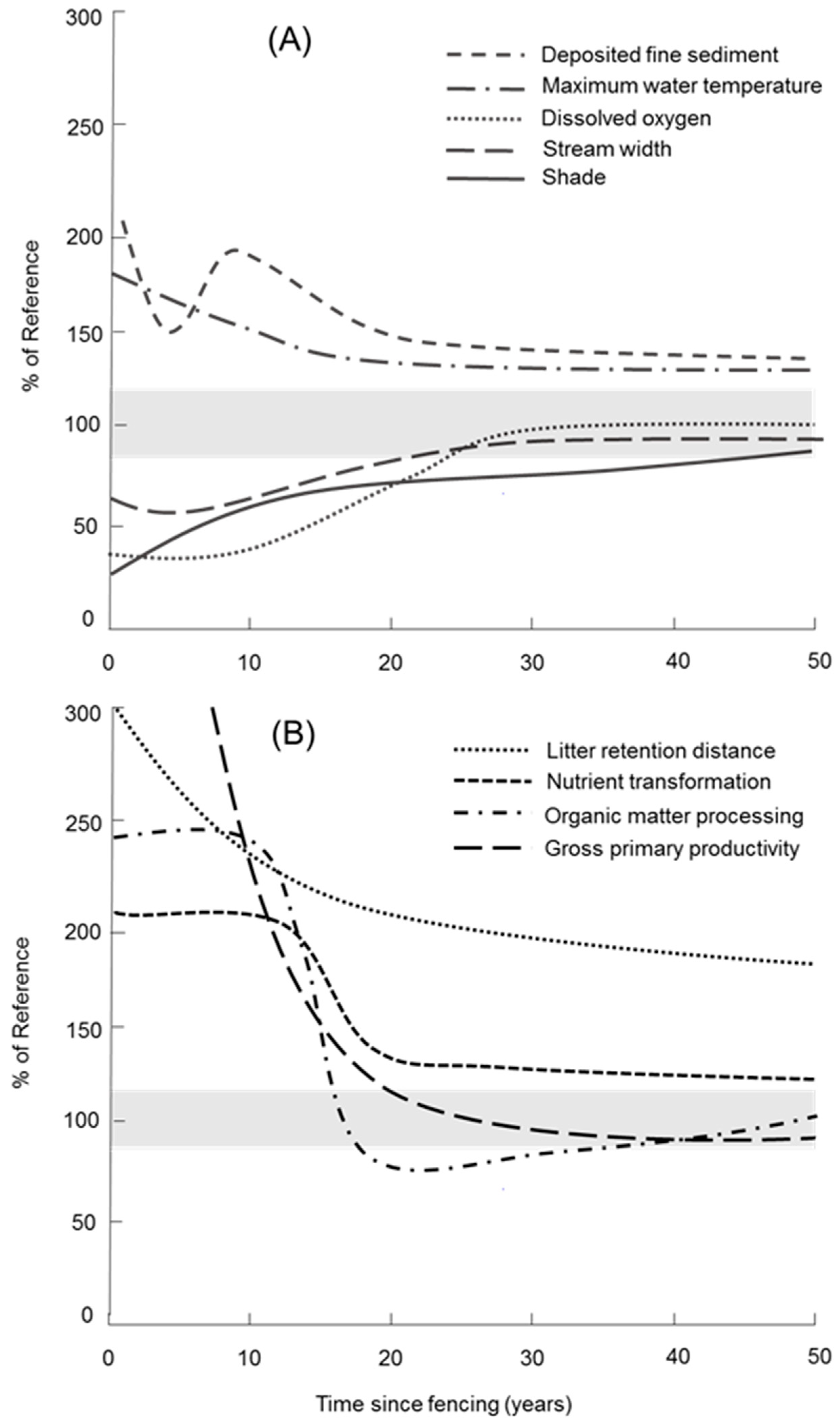
Ideally, indicators of stream ecosystem health are sensitive to change in human actions over time, such as restoration. While the primary focus of the above studies has been to quantify the response of functional indicators to land use effects, there is little if any, scientific evidence on the suitability of functional measures as indicators of restoration success [46,47]. Functional indicators are responsive to a range of reach-scale and catchment-scale drivers [48], and as such may be useful for discerning the optimum design of restoration methods to improve stream health. Further, functional indicators are predicted to respond to streamside fencing variably over time (Figure 1) following the restoration of physical metrics and other drivers discussed above. Multiple functional indicators may therefore be required to assess the restorative effect of fencing on stream functioning, considering the multidimensional character of stream function as well as its temporal character.
The overall objective of this study was to assess the effectiveness of streamside fencing at a reach scale to restore stream function. We measured a range of functional metrics to indicate potential restoration recovery trajectories in the retention, transformation and absorption of nutrients and carbon into stream food-webs. Functional metrics, including GPP, ER, wood mass loss, cotton strip decomposition, organic matter retention, and δ15N values of primary consumers, were measured alongside metrics describing physical stream habitat and water quality. Potential recovery trajectories were explored by surveying 11 pairs of sites, with and without riparian buffers fenced between five to 34 years previously in the central North Island, New Zealand. Overall, we expected to see a shift in stream function from impacted states for unfenced sites (i.e., “poor” ecosystem health) to less-impacted states for fenced sites (i.e., “healthy” ecosystem health). We hypothesised that
(1) fencing would improve the state of ecosystem health as described by physical and functional indicators due to riparian re-establishment, leading to a higher proportion of shade, lower average water temperature, greater hydraulic retention, decreased rates of GPP and ER, decreased organic matter processing rates, and decreased δ15N values indicative of more efficient biogeochemical cycling and
(2) time since fencing would lead to a greater difference between fenced and unfenced sites as described by physical and functional indicators of ecosystem health, hence illustrating a ‘rubber-band’ model of recovery.
2. Materials and Methods
2.1. Study Sites and Design
Our study was conducted in the Waikato region of the central North Island, New Zealand between March 2011 and April 2012. All measurements were conducted during stable weather conditions in autumn, when streams are generally most stressed due to sustained low flows and warmer temperatures. We sampled 11 pairs of fenced and unfenced stream reaches to assess the effects of riparian fencing on stream health. Fenced reaches had been retired and fenced from adjacent grazed land between 5 and 34 years previously (Table 1), and stocking rates were consistent among unfenced sites. Fenced stream reaches were either located upstream (Raglan and Whatawhata) or downstream of unfenced stream reaches (Waitetuna, Waitomo, Mangawhara, Matarawa, Tapapakanga, Little Waipa and Waitete). At two sites, fenced and unfenced reaches were located on neighbouring, but different streams (Taupo & Kakahu), due to the difficulty of finding fenced sites equal or greater than 30 years old adjacent to grazed sites. Nine of the 11 pairs had been previously studied by Parkyn et al. [7] to test the effectiveness of fenced riparian buffers on biological and water quality indicators.
Catchment size ranged from just over 300 ha to 8600 ha (Whatawhata Stream and Little Waipa River, respectively; Table 1) as determined from the Freshwater Environments of New Zealand database, FENZ, [50]. Eight of the 11 study pairs were located in catchments with high-producing exotic grassland as the predominant land cover upstream and two study pairs with either exotic or indigenous forest, LCDB, [51]. Kakahu was the only site where predominant land use differed between Treatments, with high-producing exotic grassland at the fenced reach and indigenous forest at the unfenced reach.
The length of fenced reaches ranged from 480 m (Raglan) to 1700 m (Taupo) (Table 1). Fenced stream length as a proportion of total upstream length ranged from 0.1% (Kakahu) to 33.1% (Matarawa; Table 1). Riparian vegetation, other than grass, was present at both fenced and unfenced sites, except at unfenced Waitete, Kakahu and Taupo sites. Where riparian vegetation other than grass was present, mean vegetation buffer widths ranged from 0.6 m (Mangawhara fenced) to 75 m (Taupo fenced; Table 1) and were wider at the fenced (mean = 23.1 m) than at the unfenced sites (mean = 5.5 m). Riparian area as a proportion of total catchment area ranged from less than 0.01% (unfenced sites at Kakahu, Waitete and Mangawhara) to 1.73% (Whatawhata fenced site; Table 1).
2.2. Physical Habitat
Study reach lengths were set by hydraulic travel times of at least 1 h from a defined upstream point within a fenced reach (see ‘Ecosystem metabolism’ below for a description of how residence time was determined). At each site, stream depth and wetted width were measured at 10 cross-sections spaced evenly along the length of the study reach to cover local variation in channel morphology. Discharge was measured on a single occasion at the downstream end of each study reach using a 2D FlowTracker Handheld Acoustic Doppler Velocimeter® (SonTek YSI, San Diego, CA, USA). Stream bed particle size distribution (including occurrence of wood) was measured using the pebble count method of Wolman [52] and the amount of in-stream macrophyte cover (emergent or submerged) was estimated in a 1-m-wide transect extending upstream of each of the 10 cross-sections. Riparian buffer width was measured on both sides of the stream at 5 cross-sections along each study reach. Stream shade was estimated visually at water level at three random points across the channel at each cross-section.
2.3. Functional Indicators
2.3.1. Organic Matter Retention
We assessed the retention capacity of stream reaches in April 2011 by using analogues of coarse particulate organic matter (CPOM) following the methodology of Quinn, Phillips and Parkyn [32]. For this, we used conditioned ginkgo (Ginkgo biloba) leaves soaked overnight to make them neutrally buoyant [53], waterproof paper triangles (4.4 cm sides) and pine dowels (30 cm long, 1 cm diameter, after Webster et al. [54] as standard CPOM types. The leaf analogues represented structurally distinct leaf types found naturally in litter fall, including freshly fallen floating leaves (triangles) and litter that had been in the stream long enough to become water saturated (ginkgo). Wood dowels were used to represent small branches.
We released 30 of each CPOM type at regular intervals across the wetted channel at the upstream end of each reach [55]. Triangles were released first, then ginkgo leaves, followed by dowels to avoid the larger dowels catching smaller analogues. Once it became clear that the analogues had been retained (minimum of 10 min), we recorded the distance travelled for each analogue. We characterised the object it was retained on including streambed type and size, leaf litter and wood, riparian and in-stream vegetation or hydraulic habitat type (pool, riffle, run).
Retention was calculated for each release of each CPOM type and averaged by type for multiple releases within a site as deposition velocity (Vdep, mm s−1), which is a retention measure accounting for the effects of stream size [56]:
Vdep = mean depth (mm) × water velocity (m s−1)/mean travel distance (Sp, m)
Organic matter retention was measured for all analogues at all sites, except at Waitetuna where triangles could not be retrieved post release due to high water depth and turbidity.
2.3.2. Ecosystem Metabolism
We estimated the combination of gross primary production (GPP) and ecosystem respiration (ER) for each paired site using Odum’s open-system two-station analysis of diel oxygen curves [57], as modified by Marzolf et al. [58]. This required measurements of the diel changes in dissolved oxygen (DO) saturation at the upstream and downstream ends of each reach [59].
At each paired site, DO saturation and water temperature were continuously recorded with optical fluorescence probes (D-Opto, Zebra-Tech Ltd, Nelson, New Zealand) during stable flows at 15-min intervals for at least a 48-h period during March and April 2012. Paired sites were recorded simultaneously. Prior to data recording, the oxygen probes were calibrated in air-saturated water at sea level. To determine the differences in the calibration resulting from instrument drift and between sondes, all loggers were deployed together for one hour at the beginning of each recording period so that any differences could be corrected before data analysis. To measure hydraulic travel times between upstream and downstream DO loggers (aimed at a minimum of 1 hour), we released 50 mL of Rhodamine® WT liquid dye across the stream width upstream of the upper DO sonde and tracked water travel time by monitoring Rhodamine® concentrations at the downstream DO sonde with a C3TM Submersible Field Fluorometer (Turner Designs, San Jose, CA, USA).
The rate of ER and the re-aeration coefficient (k) were determined following the methods from Young & Huryn [59], except k was estimated using the night-time regression method [60] instead of using tracer gases. This method assumes low surface turbulence, as was the case in this study. The ratio of GPP:ER (P/R) was also determined. P/R relates to the balance between primary production and ecosystem respiration and determines whether the reach is autotrophic (P/R > 1) or heterotrophic (P/R < 1) [57].
2.3.3. Organic Matter Processing
To provide an indication of organic matter decomposition, we evaluated organic matter processing rates by measuring wood break-down (mass loss) and cellulose decomposition potential (cotton tensile strength loss). Briefly, wood break-down rates were determined by weighing birch wood (Betula platyphylla) coffee stirrer sticks pre- and postinstalment in stream water. At each paired site, five groups were deployed in riffle habitat for 90 days from April to June 2011. Wood mass loss rates were determined following Petersen and Cummins [61] using degree days (dd) as the time variable. Wood mass loss data was collected for all 11 pairs of sites, except at Mangawhara unfenced site where the temperature logger and wood sticks were lost during deployment.
Cellulose decomposition potential was measured, following Tiegs, Clapcott, Griffiths and Boulton [35], whereby five cotton replicates (Product no. 222; EMPA, St. Gallen, Switzerland) were deployed at each site for seven days in April 2011. Cotton tensile strength loss (CTSL) was reported per degree day (dd) in the same way as the wooden stick data to allow for comparison between these two measures of organic matter processing. Water temperature was continuously recorded in 15-min intervals with a Hobo pendant logger (Onset, Bourne, MA, USA) installed at the same metal stake as the wood and cotton at each site. Mean daily temperature was used to calculate organic matter processing rates per degree day.
2.3.4. Nutrient Transformation
Stable isotopes of nitrogen (N) reflect the source and transformation of N in stream systems and provide an indicator of nutrient sources and processing. The δ15N of primary consumers reflects accumulated N over weeks to months and thus provides a more holistic picture of N sources rather than a snapshot of N concentrations [61]. At each paired site, we hand-picked 10 primary consumers, either mayflies (Deleatidium sp.), shrimp (Paratya curvirostris Heller) or both, from benthic samples and preserved them in 90% isopropyl alcohol. In the laboratory, samples were rinsed with deionised water and their guts were removed and discarded prior to sample drying at 80 °C in a forced-draft oven. Ground samples were analysed in a Dumas elemental analyser interfaced to an isotope mass spectrometer (Europa Scientific Ltd, Crewe, England) to obtain δ15N values to provide an indication of N sources in each stream reach.
2.4. Data Analysis
To test the hypothesis that fencing would improve the state of ecosystem health, differences between Fenced and Unfenced sites across all age groups were assessed using paired t-tests (two-sample for mean). To test the hypothesis that time since fencing would improve ecosystem health, we applied an univariate permutational analysis of variance (PERMANOVA) [62] of log (x + 1) transformed physical and functional response variables measured at a site level (n = 22). The analyses included ‘Treatment’ as a fixed factor with two levels (Fenced and Unfenced), ‘Site’ as a random factor and ‘Time since fencing’ as a continuous covariate. All tests were performed using 9999 permutations of residual under a reduced model and type I sum of squares calculated (sequential) to allow the inclusion of a continuous covariate. Hence, p-values are obtained by permutation, thus avoiding the assumption of normality [63]. Univariate PERMANOVA tests were conducted using the software PRIMER 7 [64] and the PERMANOVA add-in [65].
When there was a significant effect of Treatment on CTSL, we tested for any effects of time since fencing by fitting a second linear mixed model to the data from fenced sites only (n = 252). The model also accounted for the effects of physical variables, including slope, upstream native vegetation, catchment buffer proportion, % of fine sediment, temperature, stream depth, stream width and channel width. Initial data exploration was conducted following Zuur et al. [66]. Predictor variables were centred, scaled and Box-Cox transformed before the analyses. Because water depth was negatively correlated with slope and channel depth was positively correlated with channel width they were dropped from the model (VIF > 3). Site was included as a random effect in the model to account for the spatial correlation resulting from the paired nature of the sampling design. Additionally, ‘cotton strip’ was considered as a random effect nested in ‘Site’ to account for the repeated measure design. The variability of fixed and random effects justified the use of marginal pseudo-R2 (accounting for fixed effects) and conditional pseudo-R2, accounting for fixed and random effects, [67]. Model outputs were represented as partial effect plots for each predictor. Linear mixed models were fitted using the library lme4 [68] of the software R [69].
3. Results
3.1. Physical Habitat
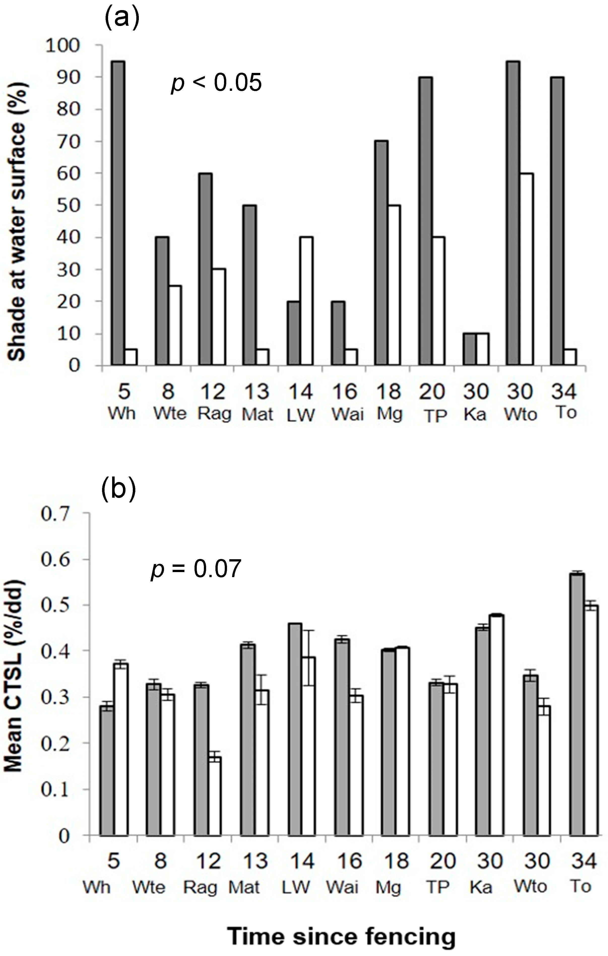
The differences in physical stream habitat were not as prominent as expected between fenced and unfenced sites. However, fenced sites had significantly wider vegetated riparian zones and higher levels of stream shading than their paired unfenced sites. Shade estimates were significantly higher for fenced (mean = 58.1%) than unfenced (mean = 25%) stream reaches (T(10) = 3.30, p < 0.05; Figure 2a; Table 2). Whatawhata and Waitomo fenced sites had the highest shading (95%; Figure 2) and the Kakahu fenced site the least shading within fenced sites (10%; Figure 2a). There was no difference in canopy height between the two treatments (T(10) = 1.34; p = 0.21) and the level of shading did not depend on time since fencing (Table 3).
Daily dissolved oxygen (DO) saturation ranged from 76.9% (Matarawa unfenced) to 128.2% (Taupo fenced) and mean DO saturation was not significantly different between fenced and unfenced sites (Table 2). Likewise, maximum daily water temperature was not influenced by treatment nor time since fencing (Table 2 and Table 3), and ranged from 10.6 °C (Taupo fenced) to 21.4 °C (Tapapakanga unfenced).
Bed substrate type was similar at fenced and unfenced sites (except at Whatawhata, Little Waipa and Tapapakanga; Table 1) with no significant differences in dominant bed substrate percentage between treatments (T(10) = 0.32, p = 0.76). Most sites had gravel (2–64 mm) as the dominant bed substrate, followed by silt (< 0.063 mm), pumice (0.063–2 mm) and then cobble (>64 mm; Table 1).
3.2. Functional Variables
3.2.1. Organic Matter Retention
Dowel and gingko analogues were primarily retained by bank vegetation (i.e., grasses, flax and ferns), with dowels generally floating on the water surface and gingko leaves being neutrally buoyant. Triangles sank to the stream bed immediately post release and were primarily retained by stream bed vegetation and substrate. Analogues had the slowest deposition velocity at the fenced Little Waipa reach (0.27 mm/s, Gingko leaves) and fastest at the fenced Waitomo reach (18.1 m/s, Triangles). There were no significant differences in deposition velocities between treatments for all analogues (Dowel T(10) = 1.4, p = 0.18, Gingko T(10) = 0.08, p = 0.93; Triangle T(10) = 0.43, p = 0.67; Table 2 and Table 3) and time since fencing did not have a significant effect on organic matter retention rates (Dowel F(1, 10) = 0.31, p = 0.62; Gingko F(1, 10) = 0.45, p = 0.52; Triangle F(1, 10) = 1.53, p = 0.25; Table 3).
3.2.2. Ecosystem Metabolism
Gross primary production ranged from 0.03 g O2/m2/d (Matarawa unfenced) to 10.9 g O2/m2/d (Little Waipa fenced; Table 2). There was no significant difference in mean GPP between the two treatments and time since fencing did not influence GPP (Table 2 and Table 3). Ecosystem respiration (ER) ranged from 0.70 g O2/m2/d (Tapapakanga unfenced) to 17.80 g O2/m2/d (Little Waipa fenced). There were no significant differences between treatments and time since fencing did not affect ER (Table 2 and Table 3).
3.2.3. Organic matter processing
Mean wood mass loss rates were slowest at the unfenced Raglan stream reach and fastest at the Kakahu unfenced stream reach (0.03%/dd and 0.13%/dd, respectively). There was no significant difference between treatments and time since fencing did not influence wood mass loss rates (Table 2 and Table 3).
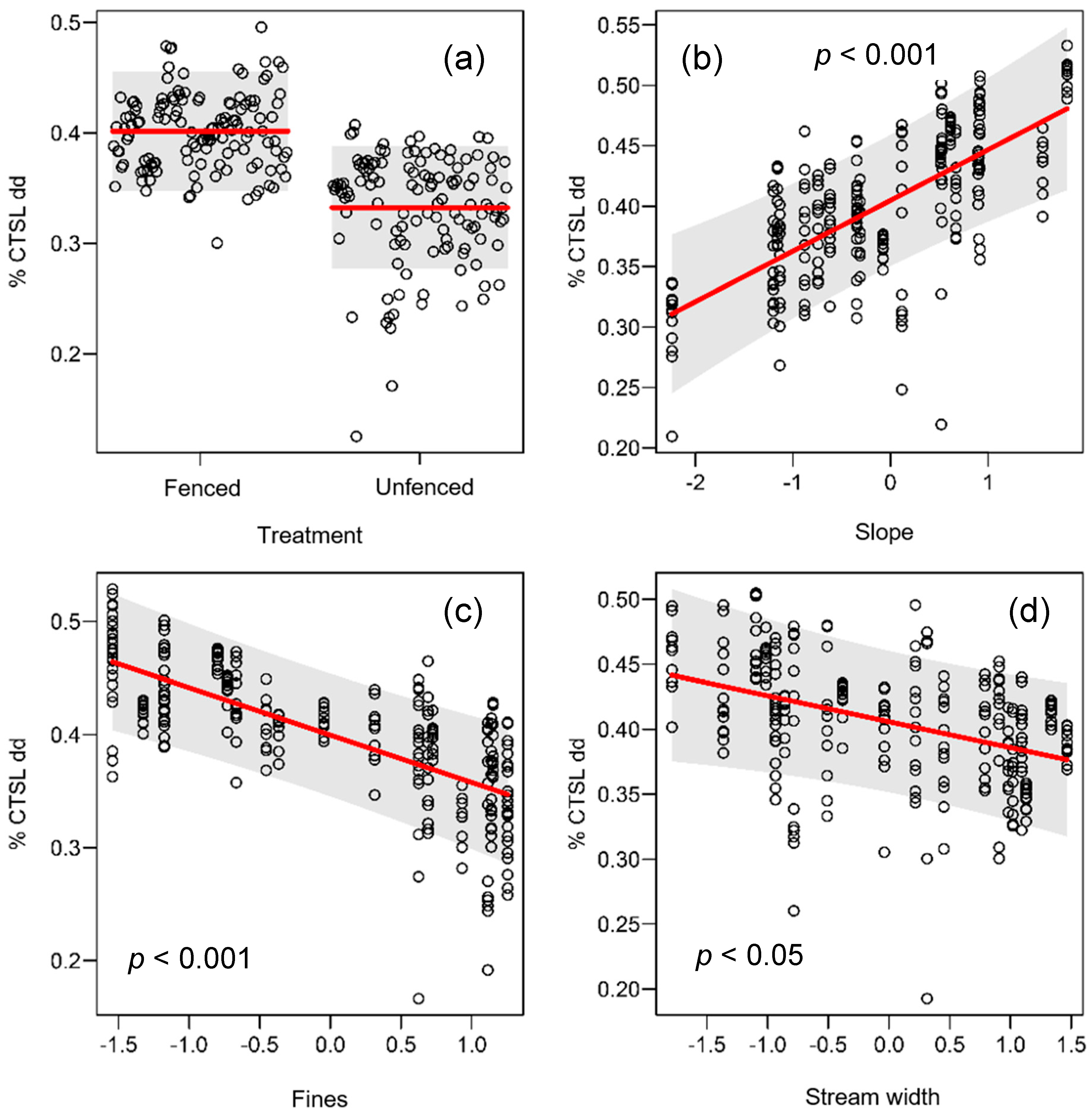
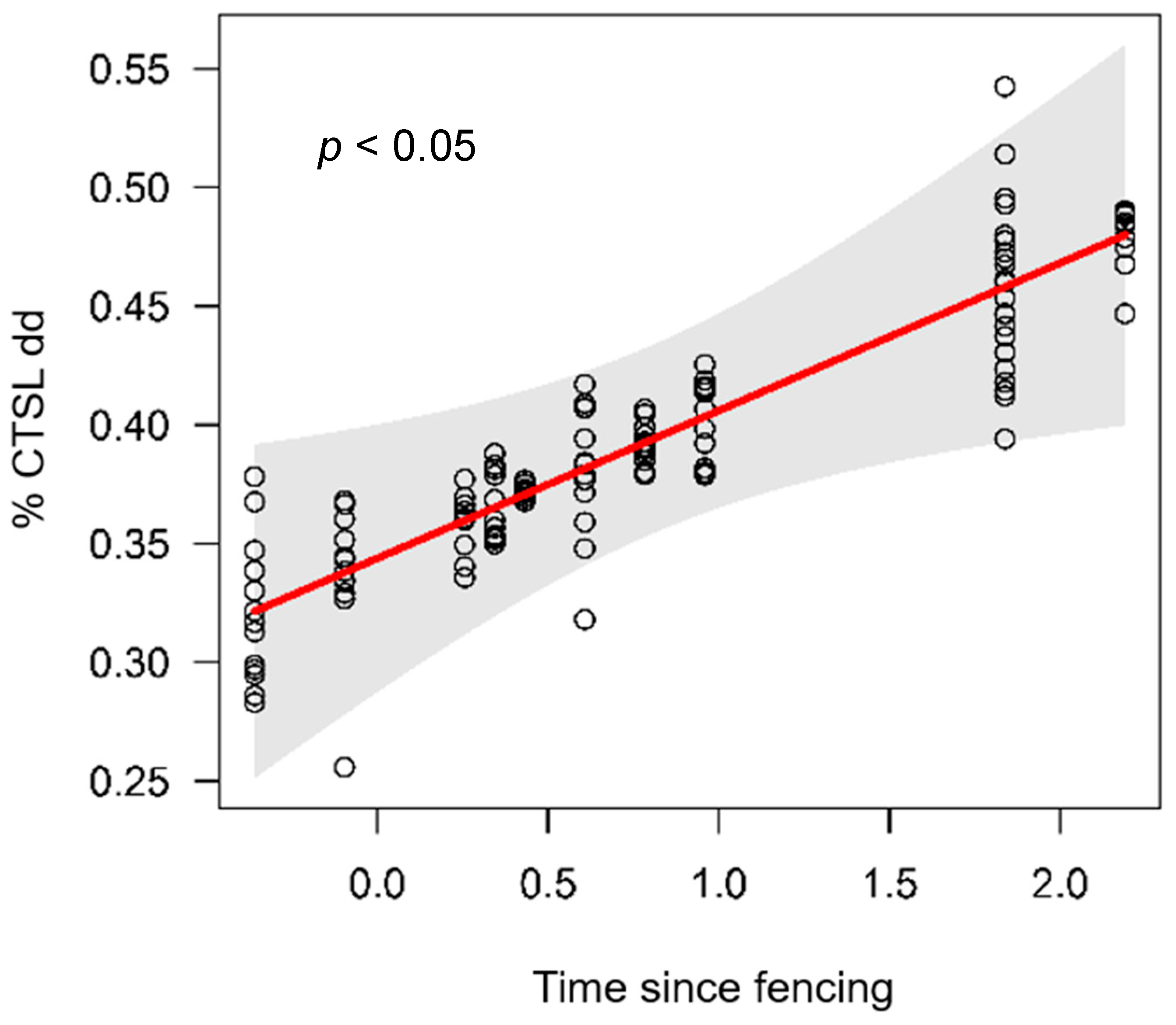
There was a strong correlation between CTSL/dd and CTSL/d (unfenced R2= 0.95, fenced R2 = 0.56) and so only results for CTSL/dd are presented. Across all sites, CTSL/dd ranged from 0.2% (Raglan unfenced) to 0.6% (Taupo fenced) (Table 2; Figure 2b). There was an indication of a treatment effect on CTSL/dd with slightly faster CTSL rates at fenced sites (mean = 0.40; Figure 3) compared to unfenced sites (mean = 0.34; Figure 3), but there was no significant difference between treatments (i.e., p = 0.07; Table 2). Slope had a positive effect on CTSL/dd, whereas both fine sediment and stream width had a negative effect on CTSL/dd (Figure 3). There was a significant positive effect of time since fencing on CTSL/dd within fenced sites (Figure 4). The fixed effect part of the model (i.e., Time since fencing) accounted for 32% of the variability in the data (marginal pseudo-R2), whereas the random and fixed effect models combined explained 91% of the variation of the CTSL/dd data.
3.2.4. Nutrient transformation
4. Discussion
In our study, we tested the effect of restoration on stream health with a focus on improved ecosystem function as an outcome. We expected to see improvements in stream ecosystem health (i.e., from modified to less modified) for several of the 19 physical and functional indicator variables measured in our study. However, only shade showed a significant difference between treatments, with higher shading observed at fenced than at unfenced sites. Our results agree with Clary [70] who found that stream shade responds reasonably quickly (i.e., 5–10 years) to livestock exclusion (for example through fencing) and the subsequent establishment of canopy cover. But because fencing is a well-recognised restoration technique for physical water quality indicators [7,8,9], we were surprised to see that the majority of physical measures was unresponsive to our treatment. In a previous study of nine of our 11 paired sites, positive improvements in water clarity and channel stability had been observed between five and 20 years following fencing [7]. These previous results suggest that our study design is sufficient to detect physical changes in stream health in the medium term, but does not necessarily account for temporal and spatial variation in physical and functional responses in the medium to long term.
With regards to process-based restoration, because there are few restoration activities that are explicitly designed to restore river processes [71], there is very little scientific evidence on the response of functional measures to restoration to date [30,47,72]. For example, Giling et al. [30] detected only marginal evidence of decreased GPP at replanted reaches compared to untreated reaches, despite an increase in canopy cover. In our study, both fenced and unfenced stream reaches displayed a range of stream health from ‘poor’ to ‘healthy’ condition according to Young et al. (2018). Surprisingly, a significant treatment effect on GPP was not observed in relation to the significant treatment effect on shade. Our data did not support hypothetical recovery trajectories (Figure 1) that predict diverse yet parallel recovery for physical and functional variables. Although, our analysis tested for predominantly linear responses over time and not the nonlinear trajectories predicted for deposited sediment (due to bank collapse as streams wide following fencing) or organic matter processing (due to change in organic matter input). In terms of restoration, this raises the interesting question whether stream structure needs to be restored first before improvements in stream function can be found, or if restoration of structure and function can happen simultaneously?
Of the eight functional indicators measured, cotton tensile-strength loss was the only one that responded to fencing, correlated with stream bed slope, stream width and fine sediment load. Streams with well-established bank and riparian vegetation generally have higher stream bank stability and substrate stability [73,74], which in turn reduces the physical effects of sediment flushing on microbial communities. Considering that volcanic pumice and silt are dominant substrates in our study catchments, smothering of microbes or impacting on macroinvertebrate habitat might explain the observed reduction of CTSL [75,76,77]. On the other hand, fine sediment can bind nutrients and consequently cotton breakdown has been shown to be faster at sites with higher sediment input due to elevated nutrients [36]. However, we did not observe any such quasi-nutrient effects, suggesting that the inhibitory physical effects of sediment were more important than sediment nutrient concentrations for CTSL in our study. In general, leaf litter breakdown rates, and in particular CTSL, are lower in streams with high levels of deposited fine sediment input [18,39,78].
Our results suggest that CTSL is also likely to increase as the streambed gets steeper and decrease as streams get wider, though it is not clear to us how these relationships relate to stream fencing. Parkyn et al. [79] demonstrated how stream widening can occur following the establishment of riparian buffers in similar agricultural streams. However, bed gradient is driven by catchment-scale rather than reach-scale processes. We did not conduct any longitudinal analysis, specifically testing for the overriding effect of the catchment on our findings. A clear avenue for future restoration studies is to view functional responses in the context of catchment-scale drivers.
Other than cotton-tensile strength loss, none of the other functional indicators measured showed a significant response to streamside fencing. This may be due to the one-off nature of sampling, with each indicator measured on a single day (or two days for ecosystem metabolism). Previous studies have shown high day-to-day variability in stream functions [80,81] that if not considered may be greater than the variation due to fencing effects. In contrast, cotton strips are deployed for seven days providing a time-integrated treatment effect on organic matter processing. However, by this logic, wooden sticks which were deployed for 90 days should also have responded significantly to the treatment, and likewise the δ15N of primary consumers should provide a time-integrated indicator of nutrient transformation. Instead, our results highlight the high spatial variability in stream function and suggests that to properly test the effectiveness of streamside fencing on stream function, greater spatial and, or temporal sampling is required.
The lags and legacies constraining restoration outcomes are well recognised [14,82], so, after 30 years, we expected to see a change in stream health from impacted to less-impacted as fenced riparian buffers aged. Cotton tensile-strength loss significantly increased with time since fencing, most likely driven by increased organic matter input related to increased canopy cover up to a certain stream size (7 m in our study). Energy pathways in smaller streams, such as in our study, are supported largely by allochthonous organic matter [83], so small streams without riparian vegetation are likely to experience a lack of organic matter input and hence a lack of organic matter cycling. We, therefore, suggest that fencing is a suitable restoration technique to assist in the establishment of microbial communities through riparian leaf litter input in small streams, facilitating the recovery of stream ecosystem health. But we also highlight the phenomenon of hysteresis during stream restoration through the re-establishment of riparian vegetation post fencing and the associated long timeframes until quantifiable benefits to stream ecosystem health can be detected.
We were unable to demonstrate any effects of time since treatment for any of the physical variables tested. Shading was significantly greater at fenced sites, but time since fencing had no effect on the amount of shade on the water surface. In fact, Whatawhata (our ‘youngest’ fenced site) showed the highest shade records of all sites, while shading at Kakahu (one of our ‘oldest’ fenced sites) was the same at fenced and unfenced stream reaches. This high site-to-site variability was evident for most variables tested, and for most sites it was not possible to infer a link between restoration effort and a given response variable. This is not unusual in studies which aim to quantify restoration success on a reach-scale, while degradation occurs at the catchment-scale [71]. For example, Giling et al. [84] found that macroinvertebrates showed no response up to 22 years after replanting at the reach-scale due to the overriding effects of catchment-scale degradation.
Our study is unique in that it assessed the response of both functional and physical indicators of stream health to restoration over more than three decades. We hypothesised that a change in stream function would occur, indicative of improving stream health, over time and increasing spatial scales. However, our data did not follow a linear or ‘rubber band’ pattern of improvement. Tiegs et al. [35] found large variations in cotton strip tensile-strength loss among the three regions studied and among the streams within those regions, suggesting sensitivity to variation in sub-catchment and catchment-scale environmental conditions. Natural environmental variation could moderate the effects of land use and restoration efforts on stream health. In-stream habitat structure and organic matter inputs are determined primarily by local conditions such as vegetation cover at a site, whereas nutrient supply, sediment delivery, hydrology and channel characteristics are influenced by regional conditions, including landscape features and land use / cover at some distance upstream and lateral to stream sites [85]. Considering that habitat degradation often occurs at catchment scales, considerable restoration at larger scales may be required before any improving stream ecosystem responses to restoration can be seen at a reach scale [13,71]. Reach-scale restoration has been shown to have very little to no effects on biological indicators [7,12,86], however, it is well documented that width, continuous canopy and length of forested riparian zones determine the effectiveness of restoration of stream structure [87,88,89,90,91]. As for functional responses, Giling, Grace, Mac Nally and Thompson [30] demonstrated marginally improved ecosystem metabolism 17 years after riparian restoration in stream reaches shorter and narrower than ours and they suggested that metabolic response would take longer and be less pronounced in larger channels. Our results suggest that after 34 years metabolic recovery to a ‘healthy’ state may still not be achieved by passive riparian restoration via streamside fencing.
Regarding the proportion of study reaches within a catchment, our data indicated that fenced catchment proportions around 1% are likely to have some beneficiary effects on stream health. For example, shade, organic matter retention rates and water temperature for the fenced Whatawhata reach (5 years old; 1.73% of total catchment proportion) and the fenced Taupo reach (34 years old; 1.02% of total catchment proportion) pointed towards an improvement in these variables. One percent was the highest proportion within a catchment area that was fenced in our study, and we suggest that any proportion of riparian vegetation > 1% of total catchment area may have a positive effect on stream health, independent of the establishment age. In a study conducted 10 years earlier on the same sites, significant improvements in visual water clarity and channel stability were observed [7]. Similarly, Holmes [20] identified a minimum 1 km length of 5-m-wide riparian vegetation was required to improve habitat heterogeneity in small agricultural streams. We recommend further research on the effects of small-scale restoration (that is treatment size of 1%–10% of the total catchment area) on functional metrics to elucidate the optimal restoration effort to achieve improved ecosystem health in agricultural streams. Future research should include (1) increased temporal sampling to characterise restoration trajectories and improve sample size, as our study constitutes a single post restoration sample for each pair of sites; (2) concurrent measurement of riparian structure (e.g., floristic composition), channel and in-stream morphology, water quality and biological characteristics, alongside functional indicators of biophysical processes, to elucidate the relationship between structural and functional restoration; and (3) improved definition of the restoration treatment within the catchment (e.g., placement, relative scale and level of active management), to inform the optimal design of future riparian restoration. Space-for-time analysis did not yield the results we initially had hypothesised, emphasising the complex pathway of stream restoration from fencing and the ongoing need for an integrated assessment approach. This means functional as well as physical and biological structural variables need to be included in monitoring of long-term restoration efforts (>30 years) to successfully determine if an improvement in stream health has occurred.
In conclusion, our comparison of 11 paired small streams in central North Island of New Zealand showed that of the 19 physical and functional variables that were tested, only cotton tensile-strength loss and stream shade were higher within fenced sites compared to unfenced sites. This indicates that fencing is likely to influence stream ecosystem function; however, restoration needs to be at a sufficient scale, before any observable effects can be made. Small-scale (<2% of the upstream catchment area) efforts to fence the riparian zones of streams appear to have little effect on ecosystem function and we strongly emphasize the confounding effects of large site-to-site variability and the overriding effects of catchment degradation on reach-scale restoration.
Author Contributions
Conceptualization, R.G.Y.; methodology, K.D., R.G.Y, J.E.C.; formal analysis, K.D., J.E.C.; investigation, K.D.; writing, K.D., J.E.C., R.G.Y.
Funding
This research was funded by Ministry of Science and Innovation, contract number CONC-20599.
Acknowledgments
We thank all the landowners that allowed us to conduct this study on their land: Martin Koning, Sarah and Mike Moss, Colleen Hawkes, Neil Board, Jocelyn, Marc and Sarah Newton, the Van Loon Family, Matthew Wood, Phil Guest, Les and Fern Bennett, Bruce and Christine Lane, Roger and Eunice, Andrew Jenks, Auckland Council and the Department of Conservation, and apologize to those we have missed. We also thank John Quinn, David Reid, Aslan Wright-Stow, Kerry Costley, Toni Johnston and Josh de Villiers for help in the field and provision of some data. We thank Javier Atalah for assistance with the statistical analyses and three anonymous reviewers for their review of this manuscript.
Conflicts of Interest
The authors declare no conflict of interest.
References
- Bernhardt, E.S.; Palmer, M.A.; Allan, J.D.; Alexander, G.; Barnas, K.; Brooks, S.; Carr, J.; Clayton, S.; Dahm, C.; Follstad-Shah, J.; et al. Synthesizing U.S. River restoration efforts. Science 2005, 308, 636–637. [Google Scholar] [CrossRef] [PubMed]
- Roni, P.; Hanson, K.; Beechie, T. Global Review of the Physical and Biological Effectiveness of Stream Habitat Rehabilitation Techniques. N. Am. J. Fish. Manag. 2008, 28, 856–890. [Google Scholar] [CrossRef]
- Pedersen, M.L.; Andersen, J.M.; Nielsen, K.; Linnemann, M. Restoration of Skjern River and its valley: Project description and general ecological changes in the project area. Ecol. Eng. 2007, 30, 131–144. [Google Scholar] [CrossRef]
- ICPR. Action Plan on Floods 1995–2005—Action Targets, Implementation and Results; Brochure, Abridged Version of Technical Report No. 156; ICPR: Koblenz, Germany, 2007; p. 16. ISBN 3-935324-63-4. [Google Scholar]
- Schwarz, U. Assessment of the Restoration Potential along the Danube and MAIN Tributaries; Final Draft; WWF International, Danube-Carpathian Programme: Vienna, Austria, May 2010. [Google Scholar]
- McKergow, L.A.; Matheson, F.E.; Quinn, J.M. Riparian management: A restoration tool for New Zealand streams. Ecol. Manag. Restor. 2016, 17, 218–227. [Google Scholar] [CrossRef]
- Parkyn, S.M.; Davies-Colley, R.J.; Halliday, N.J.; Costley, K.J.; Croker, G.F. Planted riparian buffer zones in New Zealand: Do they live up to expectations? Restor. Ecol. 2003, 11, 436–447. [Google Scholar] [CrossRef]
- Craig, L.S.; Palmer, M.A.; Richardson, D.C.; Filoso, S.; Bernhardt, E.S.; Bledsoe, B.P.; Doyle, M.W.; Groffman, P.M.; Hassett, B.A.; Kaushal, S.S.; et al. Stream restoration strategies for reducing river nitrogen loads. Front. Ecol. Environ. 2008, 6, 529–538. [Google Scholar] [CrossRef] [Green Version]
- Bragina, L.; Sherlock, O.; van Rossum, A.; Jennings, E. Cattle exclusion using fencing reduces Escherichia coli (E. coli) level in stream sediment reservoirs in northeast Ireland. Agric. Ecosyst. Environ. 2017, 239, 349–358. [Google Scholar] [CrossRef]
- Palmer, M.; Hondula, K.; Koch, B. Ecological Restoration of Streams and Rivers: Shifting Strategies and Shifting Goals. Annu. Rev. Ecol. Evol. Syst. 2014, 45, 247. [Google Scholar] [CrossRef]
- Follstad Shah, J.J.; Dahm, C.N.; Gloss, S.P.; Bernhardt, E.S. River and Riparian Restoration in the Southwest: Results of the National River Restoration Science Synthesis Project. Restor. Ecol. 2007, 15, 550–562. [Google Scholar] [CrossRef]
- Collins, K.E.; Doscher, C.; Rennie, H.G.; Ross, J.G. The Effectiveness of Riparian ‘Restoration’ on Water Quality—A Case Study of Lowland Streams in Canterbury, New Zealand. Restor. Ecol. 2013, 21, 40–48. [Google Scholar] [CrossRef]
- Lake, P.S.; Bond, N.; Reich, P. Linking ecological theory with stream restoration. Freshw. Biol. 2007, 52, 597–615. [Google Scholar] [CrossRef]
- Suding, K.N.; Hobbs, R.J. Threshold models in restoration and conservation: A developing framework. Trends Ecol. Evol. 2009, 24, 271–279. [Google Scholar] [CrossRef] [PubMed]
- Suding, K.N. Toward an Era of Restoration in Ecology: Successes, Failures, and Opportunities Ahead. Annu. Rev. Ecol. Evol. Syst. 2011, 42, 465–487. [Google Scholar] [CrossRef] [Green Version]
- Brooks, A.; Howell, T.; Abbe, T.B.; Arthington, A. Confronting Hysteresis: Wood Based River Rehabilitation in Highly Altered Riverine Landscapes in South-Eastern Australia. Geomorphology 2006, 79, 395–422. [Google Scholar] [CrossRef]
- Rapport, D.J.; Costanza, R.; McMichael, A.J. Assessing ecosystem health. Trends Ecol. Evol. 1998, 13, 397–402. [Google Scholar] [CrossRef]
- Young, R.G.; Matthaei, C.D.; Townsend, C.R. Organic matter breakdown and ecosystem metabolism: Functional indicators for assessing river ecosystem health. J. N. Am. Benthol. Soc. 2008, 27, 605–625. [Google Scholar] [CrossRef]
- Quinn, J. Effects of Rural Land Use (Especially Forestry) and Riparian Management on Stream Habitat. N. Z. J. For. 2005, 49, 16. [Google Scholar]
- Holmes, R.; Hayes, J.; Matthaei, C.; Closs, G.; Williams, M.; Goodwin, E. Riparian management affects instream habitat condition in a dairy stream catchment. N. Z. J. Mar. Freshw. Res. 2016, 50, 581–599. [Google Scholar] [CrossRef]
- Guzha, A.C.; Rufino, M.C.; Okoth, S.; Jacobs, S.; Nóbrega, R.L.B. Impacts of land use and land cover change on surface runoff, discharge and low flows: Evidence from East Africa. J. Hydrol. Reg. Stud. 2018, 15, 49–67. [Google Scholar] [CrossRef]
- Nugroho, P.; Marsono, D.; Sudira, P.; Suryatmojo, H. Impact of Land-use Changes on Water Balance. Procedia Environ. Sci. 2013, 17, 256–262. [Google Scholar] [CrossRef] [Green Version]
- Castillo, M.M.; Morales, H.; Valencia, E.; Morales, J.J.; Cruz-Motta, J.J. The effects of human land use on flow regime and water chemistry of headwater streams in the highlands of Chiapas. Knowl. Manag. Aquat. Ecosyst. 2013. [Google Scholar] [CrossRef]
- Quinn, J.M.; Stroud, M.J. Water quality and sediment and nutrient export from New Zealand hill-land catchments of contrasting land use. N. Z. J. Mar. Freshw. Res. 2002, 36, 409–429. [Google Scholar] [CrossRef]
- Niyogi, D.K.; Simon, K.; Townsend, C.R. Breakdown of tussock grass in streams along a gradient of agricultural development in New Zealand. Freshw. Biol. 2003, 48, 1698–1708. [Google Scholar] [CrossRef]
- Von Schiller, D.; Marti, E.; Riera, J.L.; Sabater, F. Effects of nutrients and light on periphyton biomass and nitrogen uptake in Mediterranean streams with contrasting land uses. Freshw. Biol. 2007, 52, 891–906. [Google Scholar] [CrossRef]
- Violin, C.R.; Cada, P.; Sudduth, E.B.; Hassett, B.A.; Penrose, D.L.; Bernhardt, E.S. Effects of urbanization and urban stream restoration on the physical and biological structure of stream ecosystems. Ecol. Appl. A Publ. Ecol. Soc. Am. 2011, 21, 1932. [Google Scholar] [CrossRef]
- Shilla, D.J.; Shilla, D.A. The effects of catchment land use on water quality and macroinvertebrate assemblages in Otara Creek, New Zealand. Chem. Ecol. 2011, 27, 445–460. [Google Scholar] [CrossRef]
- Tank, J.L.; Rosi-Marshall, E.J.; Griffiths, N.A.; Entrekin, S.A.; Stephen, M.L. A review of allochthonous organic matter dynamics and metabolism in streams. J. N. Am. Benthol. Soc. 2010, 29, 118–146. [Google Scholar] [CrossRef] [Green Version]
- Giling, D.P.; Grace, M.R.; Mac Nally, R.; Thompson, R.M. The influence of native replanting on stream ecosystem metabolism in a degraded landscape: Can a little vegetation go a long way? Freshw. Biol. 2013, 58, 2601–2613. [Google Scholar] [CrossRef]
- Clapcott, J.E.; Young, R.G.; Goodwin, E.O.; Leathwick, J.R. Exploring the response of functional indicators of stream health to land-use gradients. Freshw. Biol. 2010, 55, 2181–2199. [Google Scholar] [CrossRef]
- Quinn, J.M.; Phillips, N.R.; Parkyn, S.M. Factors influencing retention of coarse particulate organic matter in streams. Earth Surf. Process. Landf. 2007, 32, 1186–1203. [Google Scholar] [CrossRef]
- McTammany, M.E.; Benfield, E.F.; Webster, J.R. Recovery of stream ecosystem metabolism from historical agriculture. J. N. Am. Benthol. Soc. 2007, 26, 532–545. [Google Scholar] [CrossRef]
- Webster, J.R.; Benfield, E.F. Vascular plant breakdown in freshwater ecosystems. Annu. Rev. Ecol. Syst. 1986, 17, 567–594. [Google Scholar] [CrossRef]
- Tiegs, S.D.; Clapcott, J.; Griffiths, N.; Boulton, A.J. A standardized cotton strip assay for measuring organic-matter decomposition in streams. Ecol. Indic. 2013, 32, 131–139. [Google Scholar] [CrossRef]
- Boulton, A.; Quinn, J. A simple and versatile technique for assessing cellulose decomposition potential in floodplain and riverine sediments. Arch. Fur Hydrobiol. 2000, 150, 133–151. [Google Scholar] [CrossRef]
- Griffiths, N.A.; Tiegs, S.D. Organic-matter decomposition along a temperature gradient in a forested headwater stream. Freshw. Sci. 2016, 35, 518–533. [Google Scholar] [CrossRef]
- Vyšná, V.; Dyer, F.; Maher, W.; Norris, R. Cotton strip decomposition rate as a river condition indicator–Diel temperature range and deployment season and length also matter. Ecol. Indic. 2014, 45, 508–521. [Google Scholar] [CrossRef]
- Bierschenk, A.; Savage, C.; Townsend, C.; Matthaei, C. Intensity of land use in the catchment influences ecosystem functioning along a freshwater-marine continuum. Ecosystems 2012, 15, 637–651. [Google Scholar] [CrossRef]
- Udy, J.W.; Fellows, C.S.; Bartkow, M.E.; Bunn, S.E.; Clapcott, J.E.; Harch, B.D. Measures of nutrient processes as indicators of stream ecosystem health. Hydrobiologia 2006, 572, 89–102. [Google Scholar] [CrossRef]
- Mulholland, P.J.; Webster, J. Nutrient dynamics in streams and the role of J-NABS. J. N. Am. Benthol. Soc. 2010, 29, 100–117. [Google Scholar] [CrossRef]
- Von Schiller, D.; Acuña, V.; Aristi, I.; Arroita, M.; Basaguren, A.; Bellin, A.; Boyero, L.; Butturini, A.; Ginebreda, A.; Kalogianni, E.; et al. River ecosystem processes: A synthesis of approaches, criteria of use and sensitivity to environmental stressors. Sci. Total Environ. 2017, 596–597, 465–480. [Google Scholar] [CrossRef]
- Diebel, M.W.; Zanden, M.J.V. Nitrogen stable isotopes in streams: Effects of agricultural sources and transformations. Ecol. Appl. 2009, 19, 1127–1134. [Google Scholar] [CrossRef] [PubMed]
- Udy, J.W.; Bunn, S.E. Elevated δ15N values in aquatic plants from cleared catchments: Why? Mar. Freshw. Res. 2001, 52, 347–351. [Google Scholar] [CrossRef]
- Hamilton, S.; Tank, J.; Raikow, D.; Wollheim, W.; Peterson, B.; Webster, J. Nitrogen uptake and transformation in a midwestern U.S. stream: A stable isotope enrichment study. Biogeochemistry 2001, 54, 297–340. [Google Scholar] [CrossRef]
- Rubin, Z.; Kondolf, G.M.; Rios-Touma, B. Evaluating Stream Restoration Projects: What Do We Learn from Monitoring? Water 2017, 9, 174. [Google Scholar] [CrossRef]
- Sudduth, E.B.; Hassett, B.A.; Cada, P.; Bernhardt, E.S. Testing the Field of Dreams Hypothesis: Functional responses to urbanization and restoration in stream ecosystems. Ecol. Appl. 2011, 21, 1972–1988. [Google Scholar] [CrossRef] [PubMed]
- Sheldon, F.; Peterson, E.E.; Boone, E.L.; Sippel, S.; Bunn, S.E.; Harch, B.D. Identifying the spatial scale of land use that most strongly influences overall river ecosystem health score. Ecol. Appl. 2012, 22, 2188–2203. [Google Scholar] [CrossRef] [PubMed]
- Parkyn, S.; Collier, K.; Clapcott, J.; David, B.; Davies-Colley, R.; Matheson, F.; Quinn, J.; Shaw, W.; Storey, R. The Restoration Indicators Toolkit: Indicators for Monitoring the Ecological Success of Stream Restoration; National Institute of Water and Atmospheric Research: Hamilton, New Zealand, 2010; p. 134. Available online: http://www.envirolink.govt.nz/assets/Envirolink/RestorationIndicatorToolkit-stream.pdf (accessed on 20 June 2019).
- Leathwick, J.R.; West, D.; Gerbeaux, P.; Kelly, D.; Robertson, H.; Brown, D.; Chadderton, W.L.; Ausseil, A.-G. Freshwater Ecosystems of New Zealand (FENZ) Database; Department of Conservation: Wellington, New Zealand, 2010.
- Ministry for the Environment. The New Zealand Land Cover Database (LCDB) 4; Ministry for the Environment: Wellington, New Zealand, 2014.
- Wolman, M.G. A method of sampling coarse river-bed material. Trans. Am. Geophys. Union 1954, 35, 951–956. [Google Scholar] [CrossRef]
- Speaker, R.; Moore, K.; Gregory, S. Analysis of the process of retention of organic matter in stream ecosystems. Verh. Int. Ver. Fuer Theor. Angew. Limnol. 1984, 22, 1835–1841. [Google Scholar] [CrossRef]
- Webster, J.R.; Covich, A.P.; Tank, J.L.; Crockett, T.V. Retention of coarse organic particles in streams in the southern Appalachian Mountains. J. N. Am. Benthol. Soc. 1994, 13, 140–150. [Google Scholar] [CrossRef]
- James, A.B.W.; Henderson, I.M. Comparison of coarse particulate organic matter retention in meandering and straightened sections of a third-order New Zealand stream. River Res. Appl. 2005, 21, 641–650. [Google Scholar] [CrossRef]
- Brookshire, E.N.J.; Dwire, K.A. Controls on patterns of coarse organic particle retention in headwater streams. J. N. Am. Benthol. Soc. 2003, 22, 17–34. [Google Scholar]
- Odum, H.T. Primary production in flowing waters. Limnol. Oceanogr. 1956, 1, 102–117. [Google Scholar] [CrossRef]
- Marzolf, E.R.; Mulholland, P.J.; Steinman, A.D. Improvements to the diurnal upstream-downstream dissolved oxygen change technique for determining whole-stream metabolism in small streams. Can. J. Fish. Aquat. Sci. 1994, 51, 1591–1599. [Google Scholar] [CrossRef]
- Young, R.G.; Huryn, A.D. Effects of land use on stream metabolism and organic matter turnover. Ecol. Appl. 1999, 9, 1359–1376. [Google Scholar] [CrossRef]
- Owens, M. Measurements on non-isolated natural communities in running waters. In A Manual on Methods for Measuring Primary Production in Aquatic Environments; Vollenweider, R.A., Ed.; Blackwell Scientific Publications: Oxford, UK, 1974; pp. 111–119. [Google Scholar]
- Petersen, R.C.; Cummins, K.W. Leaf processing in a woodland stream. Freshw. Biol. 1974, 4, 343–368. [Google Scholar] [CrossRef]
- Anderson, M.J. Permutational test for univariate or multivariate analysis of variance and regression. Can. J. Fish. Aquat. Sci. 2001, 58, 626–639. [Google Scholar] [CrossRef]
- Anderson, M.J. Permutational Multivariate Analysis of Variance (PERMANOVA). In Wiley StatsRef: Statistics Reference Online; Balakrishnan, N., Colton, T., Everitt, B., Piegorsch, W., Ruggeri, F., Teugels, J.L., Eds.; Department of Statistics, University of Auckland: Auckland, New Zealand, 2017. [Google Scholar]
- Clarke, K.R.; Gorley, R.N. PRIMER v7: User Manual/Tutorial; Primer-E: Plymouth, UK, 2015; p. 296. [Google Scholar]
- Anderson, M.J.; Gorley, R.N.; Clarke, R.K. PERMANOVA+ for Primer: Guide to Software and Statisticl Methods; Primer-E Limited: Auckland, New Zealand, 2008. [Google Scholar]
- Zuur, A.F.; Ieno, E.N.; Elphick, C.S. A protocol for data exploration to avoid common statistical problems. Methods Ecol. Evol. 2010, 1, 3–14. [Google Scholar] [CrossRef]
- Nakagawa, S.; Schielzeth, H. A general and simple method for obtaining R² from Generalized Linear Mixed-effects Models. Methods Ecol. Evol. 2013, 4, 133–142. [Google Scholar] [CrossRef]
- Bates, D.; Mächler, M.; Bolker, B. Fitting linear mixed-effects models using lme4. J. Stat. Softw. 2015, 67. [Google Scholar] [CrossRef]
- R Core Team. A Language and Environment for Statistical Computing; R Foundation for Statistical Computing: Vienna, Austria, 2016. [Google Scholar]
- Clary, W.P. Stream Channel and Vegetation Responses to Late Spring Cattle Grazing. J. Range Manag. 1999, 52, 218–227. [Google Scholar] [CrossRef]
- Bernhardt, E.S.; Palmer, M.A. River restoration: The fuzzy logic of repairing reaches to reverse catchment scale degradation. Ecol. Appl. 2011, 21, 1926–1931. [Google Scholar] [CrossRef] [PubMed]
- Lepori, F.; Palm, D.; Malmqvist, B. Effects of stream restoration on ecosystem functioning: Detritus retentiveness and decomposition. J. Appl. Ecol. 2005, 42, 228–238. [Google Scholar] [CrossRef]
- Loades, K.W.; Bengough, A.G.; Bransby, M.F.; Hallett, P.D. Planting density influence on fibrous root reinforcement of soils. Ecol. Eng. 2010, 36, 276–284. [Google Scholar] [CrossRef]
- Boothroyd, I.K.G.; Quinn, J.M.; Langer, E.R.; Costley, K.J.; Steward, G. Riparian buffers mitigate effects of pine plantation logging on New Zealand streams: 1. Riparian vegetation structure, stream geomorphology and periphyton. For. Ecol. Manag. 2004, 194, 199–213. [Google Scholar] [CrossRef]
- Wagenhoff, A.; Townsend, C.R.; Matthaei, C.D. Macroinvertebrate responses along broad stressor gradients of deposited fine sediment and dissolved nutrients: A stream mesocosm experiment. J. Appl. Ecol. 2012, 49, 892–902. [Google Scholar] [CrossRef]
- Sponseller, R.A.; Benfield, E.F. Influences of land use on leaf breakdown in southern Appalachian headwater streams: A multiple-scale analysis. J. N. Am. Benthol. Soc. 2001, 20, 44–59. [Google Scholar] [CrossRef]
- Risse-Buhl, U.; Mendoza-Lera, C.; Norf, H.; Pérez, J.; Pozo, J.; Schlief, J. Contrasting habitats but comparable microbial decomposition in the benthic and hyporheic zone. Sci. Total Environ. 2017, 605–606, 683–691. [Google Scholar] [CrossRef]
- Piggott, J.J.; Niyogi, D.K.; Townsend, C.R.; Matthaei, C.D. Multiple stressors and stream ecosystem functioning: Climate warming and agricultural stressors interact to affect processing of organic matter. J. Appl. Ecol. 2015, 52, 1126–1134. [Google Scholar] [CrossRef]
- Parkyn, S.M.; Davies-Colley, R.J.; Cooper, A.B.; Stroud, M.J. Predictions of stream nutrient and sediment yield changes following restoration of forested riparian buffers. Ecol. Eng. 2005, 24, 551–558. [Google Scholar] [CrossRef]
- Simon, K.S.; Townsend, C.R.; Biggs, B.J.F.; Bowden, W.B. Temporal variation of N and P uptake in 2 New Zealand streams. J. N. Am. Benthol. Soc. 2005, 24, 1–18. [Google Scholar] [CrossRef]
- Clapcott, J.E.; Young, R.G.; Neale, M.W.; Doehring, K.A.M.; Barmuta, L.A. Land use affects temporal variation in stream metabolism. Freshw. Sci. 2016, 35, 1164–1175. [Google Scholar] [CrossRef] [Green Version]
- Hamilton, S.K. Biogeochemical time lags may delay responses of streams to ecological restoration: Time lags in stream restoration. Freshw. Biol. 2012, 57, 43–57. [Google Scholar] [CrossRef]
- Benfield, E.; Fritz, K.; Tiegs, S. Leaf litter Breakdown. In Methods in Stream Ecology; Elsevier: Amsterdam, The Netherlands, 2017; pp. 71–82. [Google Scholar]
- Giling, D.P.; Mac Nally, R.; Thompson, R.M. How sensitive are invertebrates to riparian-zone replanting in stream ecosystems? Mar. Freshw. Res. 2016, 67, 1500–1511. [Google Scholar] [CrossRef]
- Allan, J.D.; Erickson, D.L.; Fay, J. The influence of catchment land use on stream integrity across multiple spatial scales. Freshw. Biol. 1997, 37, 149–161. [Google Scholar] [CrossRef] [Green Version]
- Ranganath, S.C.; Hession, W.; Wynn Thompson, T. Livestock Exclusion Influences on Riparian Vegetation, Channel Morphology, and Benthic Macroinvertebrate Assemblages. J. Soil Water Conserv. 2009, 64, 33–42. [Google Scholar] [CrossRef]
- Lowrance, R. Riparian forest ecosystems as filters for non-point source pollution. In Success, Limitations, and Frontiers in Ecosystem Science; Pace, M.L., Groffman, P.M., Eds.; Springer: New York, NY, USA, 1998; pp. 113–141. [Google Scholar]
- England, L.E.; Rosemond, A.D. Small reductions in forest cover weaken terrestrial-aquatic linkages in headwater streams. Freshw. Biol. 2004, 49, 721–734. [Google Scholar] [CrossRef]
- Gore, J.A.; Shields, F.D. Can large rivers be restored? Bioscience 1995, 45, 142–152. [Google Scholar] [CrossRef]
- Storey, R.G.; Cowley, D.R. Recovery of three New Zealand rural streams as they pass through native forest remnants. Hydrobiologia 1997, 353, 63–76. [Google Scholar] [CrossRef]
- Scarsbrook, M.R.; Halliday, J. Transition from pasture to native forest land-use along stream continua: Effects on stream ecosystems and implications for restoration. N. Z. J. Mar. Freshw. Res. 1999, 33, 293–310. [Google Scholar] [CrossRef]
Figure 1.
Hypothetical trajectory of (A) physical variables and (B) functional variables in a small (<5 m wide) pastoral stream following fencing to exclude livestock from channels and riparian zones, adapted from Parkyn et al. [49]. Similar trajectories are predicted for larger streams but the time to recover to approximately 100% of reference condition (shaded area) will take longer. Note: ecosystem respiration is not plotted because despite decreasing over time values are not predicted to reach within 300% of reference condition within 50 years.

Figure 2.
Bar plots showing fenced (grey) and unfenced (white) paired stream reaches for (a) % shade and (b) % cotton tensile strength loss per degree day (CTSL/dd) ordered by time since fencing.
Figure 2.
Bar plots showing fenced (grey) and unfenced (white) paired stream reaches for (a) % shade and (b) % cotton tensile strength loss per degree day (CTSL/dd) ordered by time since fencing.

Figure 3.
Partial plots of the effects of (a) treatment, (b) slope, (c) fines and (d) stream width on % cotton tensile strength loss (CTSL) per degree day (dd) fitted using a linear mixed model for fenced and unfenced sites. Note differences in scales on the y-axes.
Figure 3.
Partial plots of the effects of (a) treatment, (b) slope, (c) fines and (d) stream width on % cotton tensile strength loss (CTSL) per degree day (dd) fitted using a linear mixed model for fenced and unfenced sites. Note differences in scales on the y-axes.

Figure 4.
The effect of time since fencing on % cotton tensile strength loss (CTSL) per degree day (dd) fitted using a linear mixed model within fenced sites.
Figure 4.
The effect of time since fencing on % cotton tensile strength loss (CTSL) per degree day (dd) fitted using a linear mixed model within fenced sites.


Table 1.
Site characteristics (describing treatment) listed according to number of years since fencing. SR = Study Reach; TCA = Total Catchment Area; Dominant bed substrate size range: silt (<0.063 mm), pumice/sand (0.063–2.00 mm), gravel (2.00–64.00 mm) and cobble (>64.00 mm).
Table 1.
Site characteristics (describing treatment) listed according to number of years since fencing. SR = Study Reach; TCA = Total Catchment Area; Dominant bed substrate size range: silt (<0.063 mm), pumice/sand (0.063–2.00 mm), gravel (2.00–64.00 mm) and cobble (>64.00 mm).
| Site (Site Code) | Treatment Fenced (F)/Unfenced (U) | Years since Fencing | SR Length (m) + SR Proportion (%) of Total Upstream River Length | SR Mean Wetted Width (m) | SR Mean Depth (m) | SR Mean Riparian Width (m) | SR Mean Discharge (L/s) | TCA (ha) + (SR Riparian Area Proportion (%) of Total Catchment Area) | Dominant Bed Substrate | Slope (%) |
|---|---|---|---|---|---|---|---|---|---|---|
| Whatawhata (Wh) | F | 5 | 560 (29.3) | 1.5 | 0.21 | 53.5 | 22.6 | 301.6 (1.73) | Silt | 0.1 |
| U | 0 | 500 (20.7) | 2.0 | 0.20 | 7.4 | 52.0 | 301.6 (0.24) | Gravel | 1.15 | |
| Waitete (Wte) | F | 8 | 900 (21.5) | 3.4 | 0.34 | 5.0 | 126.9 | 636.1 (0.03) | Cobble | 0.03 |
| U | 0 | 640 (19.5) | 5.2 | 0.33 | 0.0 | 130.3 | 636.1 (< 0.01) | Cobble | 0.17 | |
| Raglan (Rag) | F | 12 | 480 (8.5) | 1.9 | 0.15 | 36.9 | 17.9 | 619.9 (0.12) | Silt | 3.3 |
| U | 0 | 470 (7.7) | 2.0 | 0.24 | 4.9 | 14.7 | 619.9 (0.02) | Silt | 2.5 | |
| Matarawa (Mat) | F | 13 | 1100 (22.5) | 2.2 | 0.35 | 7.7 | 90.0 | 1025.3 (0.01) | Pumice | 0.10 |
| U | 0 | 1250 (33.1) | 1.8 | 0.23 | 3.7 | 69.1 | 850.9 (0.03) | Pumice | 0.46 | |
| Little Waipa (LW) | F | 14 | 670 (3.9) | 7.1 | 0.34 | 7.8 | 248.0 | 8612.5 (0.01) | Cobble | 0.27 |
| U | 0 | 994 (6.1) | 4.1 | 0.31 | 20.0 | 391.5 | 3467.2 (0.04) | Pumice | 0.73 | |
| Waitetuna (Wai) | F | 16 | 1600 (13.5) | 6.0 | 0.67 | 8.2 | 783.1 | 5568.1 (0.02) | Silt | 0.19 |
| U | 0 | 920 (8.4) | 4.4 | 0.47 | 1.8 | 604.3 | 5427.5 (0.01) | Silt | 0.11 | |
| Mangawhara (Mg) | F | 18 | 1200 (9.9) | 6.1 | 0.28 | 14.8 | 188.2 | 3151.3 (0.01) | Gravel | 0.37 |
| U | 0 | 1260 (11.5) | 6.7 | 0.27 | 0.6 | 245.0 | 3077.8 (<0.01) | Gravel | 0.82 | |
| Tapapakanga (TP) | F | 20 | 650 (0.1) | 5.8 | 0.13 | 11.4 | 140.7 | 997.4 (0.23) | Cobble | 0.87 |
| U | 0 | 1000 (18.4) | 5.5 | 0.15 | 9.9 | 173.6 | 997.4 (0.20) | Gravel | 0.12 | |
| Kakahu (Ka) | F | 30 | 1500 (11.1) | 5.7 | 0.31 | 15.3 | 604.5 | 3715.6 (0.15) | Gravel | 0.28 |
| U | 0 | 715 (0.1) | 2.8 | 0.27 | 0.0 | 151.8 | 1005.3 (< 0.01) | Gravel | 0.73 | |
| Waitomo (Wto) | F | 30 | 1200 (16.0) | 3.9 | 0.49 | 22.7 | 265.7 | 1949.6 (0.25) | Pumice | 0.15 |
| U | 0 | 1200 (17.6) | 2.6 | 0.56 | 3.6 | 287.6 | 1835.7 (0.04) | Pumice | 0.27 | |
| Taupo (To) | F | 34 | 1700 (16.0) | 2.1 | 0.18 | 75.0 | 131.5 | 3101.9 (1.02) | Gravel | 1.14 |
| U | 0 | 830 (0.1) | 1.1 | 0.21 | 0.0 | 59.6 | 387.7 (0.54) | Gravel | 0.74 |
Table 2.
Mean values and minimum/maximum ranges of variables observed (N = 11). T and p-values of paired t-test (two-sample for means) results and significance levels for the relationship between the change in fenced and unfenced sites for physical and functional indicators are also provided.
Table 2.
Mean values and minimum/maximum ranges of variables observed (N = 11). T and p-values of paired t-test (two-sample for means) results and significance levels for the relationship between the change in fenced and unfenced sites for physical and functional indicators are also provided.
| Metric | Variables | Fenced Sites | (Min–Max) | Unfenced Sites | (Min–Max) | T-value | p-value |
|---|---|---|---|---|---|---|---|
| Physical | Stream depth (m) | 0.31 | (0.13–0.67) | 0.29 | (0.15–0.56) | 0.77 | 0.46 |
| Physical | Stream width (m) | 4.11 | (1.50–7.10) | 3.50 | (1.10–6.70) | 1.34 | 0.21 |
| Physical | Channel width (m) | 10.10 | (3.10–28.70) | 9.00 | (4.8–15.91) | 0.47 | 0.64 |
| Physical | Discharge (m3/s) | 0.25 | (0.02–0.78) | 0.19 | (0.02–0.60) | 1.47 | 0.17 |
| Physical | Slope (%) | 0.62 | (0.03–3.28) | 0.80 | (0.11–2.45) | 1.23 | 0.25 |
| Physical | Silt (%) | 17.45 | (0.00-89.00) | 16.80 | (0.00–100.00) | 0.07 | 0.95 |
| Physical | Pumice/Sand (%) | 18.36 | (0.00–77.00) | 29.70 | (0.00–99.00) | 2.63 | 0.06 |
| Physical | Fines (%) | 37.36 | (1.00–91.00) | 43.80 | (1.00–100.00) | 0.63 | 0.55 |
| Physical | Shade (%) | 58.10 | (10.00–95.00) | 25.00 | (5.00–60.00) | 3.30 | <0.05 |
| Physical | Dissolved oxygen (% saturation) | 95.80 | (81.60–128.20) | 93.90 | (76.90–120.90) | 1.20 | 0.25 |
| Physical | Max daily water temperature (°C) | 14.60 | (10.60–20.20) | 14.80 | (10.70–21.40) | 0.76 | 0.46 |
| Functional | Retention dowel (Vdep; mm/s) | 3.50 | (0.30–14.90) | 1.60 | (0.60–4.10) | 1.40 | 0.18 |
| Functional | Retention gingko (Vdep; mm/s) | 2.10 | (0.27–5.90) | 2.10 | (0.50–6.00) | 0.08 | 0.93 |
| Functional | Retention triangle (Vdep; mm/s) | 5.90 | (0.80–18.1) | 6.50 | (1.70–14.4) | 0.43 | 0.67 |
| Functional | GPP (g O2/m2/day) | 3.10 | (0.10–10.9) | 2.10 | (0.03–5.20) | 1.02 | 0.33 |
| Functional | ER (g O2/m2/day) | 6.00 | (1.40–17.8) | 6.20 | (0.70–11.2) | 0.13 | 0.89 |
| Functional | Wood mass loss (%/degree day) | 0.07 | (0.04–0.10) | 0.08 | (0.03–0.13) | 1.40 | 0.19 |
| Functional | Cotton tensile strength loss (%/degree day) | 0.40 | (0.30–0.60) | 0.30 | (0.20–0.50) | 2.05 | 0.07 |
| Functional | Nutrient transformation (δ15N; ‰) | 5.60 | (3.40–9.10) | 5.80 | (3.20–9.90) | 0.28 | 0.78 |
Table 3.
Univariate permutational analysis of variance testing for effects of time since fencing, fenced vs. unfenced sites (treatment) and between sites (Site) on a range of physical and functional variables tested. Significant values (p < 0.05) are highlighted in bold.
Table 3.
Univariate permutational analysis of variance testing for effects of time since fencing, fenced vs. unfenced sites (treatment) and between sites (Site) on a range of physical and functional variables tested. Significant values (p < 0.05) are highlighted in bold.
| Physical | Stream Depth | Stream Width | Channel Width | Discharge | Slope | Shade | |||||||||||||
| df | MS | F | p | MS | F | p | MS | F | p | MS | F | p | MS | F | p | MS | F | p | |
| Time since fencing | 1 | 0.00 | 0.11 | 0.74 | 0.00 | 0.00 | 0.99 | 0.35 | 1.32 | 0.29 | 0.03 | 0.66 | 0.43 | 0.00 | 0.00 | 0.97 | 0.00 | 0.00 | 0.96 |
| Treatment | 1 | 0.00 | 0.48 | 0.51 | 0.07 | 1.63 | 0.23 | 0.00 | 0.00 | 1.00 | 0.01 | 2.01 | 0.18 | 0.14 | 4.04 | 0.08 | 5.43 | 8.73 | 0.01 |
| Site | 9 | 0.02 | 12.92 | 0.00 | 0.35 | 7.92 | 0.00 | 0.26 | 1.62 | 0.22 | 0.05 | 7.69 | 0.01 | 0.28 | 8.33 | 0.00 | 0.97 | 1.57 | 0.26 |
| Res | 10 | 0.00 | 0.04 | 0.16 | 0.01 | 0.03 | 0.62 | ||||||||||||
| Temperature | Max. Temperature | Silt | Pumice/Sand | Fines | |||||||||||||||
| df | MS | F | p | MS | F | p | MS | F | p | MS | F | p | MS | F | p | ||||
| Time since fencing | 1 | 25.41 | 1.49 | 0.23 | 0.01 | 1.43 | 0.28 | 14.80 | 3.52 | 0.09 | 8.88 | 2.14 | 0.16 | 0.02 | 0.01 | 0.95 | |||
| Treatment | 1 | 9.06 | 2.46 | 0.07 | 0.00 | 0.69 | 0.43 | 0.04 | 0.02 | 0.85 | 0.89 | 3.19 | 0.11 | 0.08 | 0.18 | 0.65 | |||
| Site | 9 | 17.06 | 4.62 | 0.00 | 0.01 | 4.89 | 0.01 | 4.21 | 2.89 | 0.06 | 4.15 | 14.80 | 0.00 | 3.96 | 8.85 | 0.00 | |||
| Res | 10 | 3.69 | 0.00 | 1.46 | 0.28 | 0.45 | |||||||||||||
| Functional | GPP | ER | Wood Mass Loss/dd | CTSL/dd | Stable Isotope | Dowel | |||||||||||||
| df | MS | F | p | MS | F | p | MS | F | p | MS | F | p | MS | F | p | MS | F | p | |
| Time since fencing | 1 | 0.02 | 0.02 | 0.88 | 0.17 | 0.30 | 0.61 | 0.00 | 1.01 | 0.33 | 0.02 | 5.18 | 0.04 | 0.06 | 0.88 | 0.37 | 0.19 | 0.31 | 0.62 |
| Treatment | 1 | 0.00 | 0.01 | 0.94 | 0.09 | 0.44 | 0.52 | 0.00 | 3.13 | 0.11 | 0.01 | 4.05 | 0.06 | 0.00 | 0.04 | 0.83 | 0.41 | 1.46 | 0.29 |
| Site | 9 | 0.74 | 2.88 | 0.06 | 0.56 | 2.72 | 0.06 | 0.00 | 1.30 | 0.11 | 0.00 | 3.20 | 0.04 | 0.07 | 0.82 | 0.61 | 0.61 | 2.15 | 0.13 |
| Res | 10 | 0.26 | 0.21 | 0.00 | 0.00 | 0.08 | 0.28 | ||||||||||||
| Gingko | Triangle | ||||||||||||||||||
| df | MS | F | p | MS | F | p | |||||||||||||
| Time since fencing | 1 | 0.26 | 0.45 | 0.52 | 0.56 | 1.53 | 0.25 | ||||||||||||
| Treatment | 1 | 0.00 | 0.01 | 0.94 | 0.12 | 0.93 | 0.35 | ||||||||||||
| Site | 9 | 0.57 | 5.41 | 0.01 | 0.37 | 2.87 | 0.08 | ||||||||||||
| Res | 10 | 0.11 | 0.13 | ||||||||||||||||
© 2019 by the authors. Licensee MDPI, Basel, Switzerland. This article is an open access article distributed under the terms and conditions of the Creative Commons Attribution (CC BY) license (http://creativecommons.org/licenses/by/4.0/).
Share and Cite
MDPI and ACS Style
Doehring, K.; Clapcott, J.E.; Young, R.G. Assessing the Functional Response to Streamside Fencing of Pastoral Waikato Streams, New Zealand. Water 2019, 11, 1347. https://doi.org/10.3390/w11071347
AMA Style
Doehring K, Clapcott JE, Young RG. Assessing the Functional Response to Streamside Fencing of Pastoral Waikato Streams, New Zealand. Water. 2019; 11(7):1347. https://doi.org/10.3390/w11071347
Chicago/Turabian StyleDoehring, Katharina, Joanne E. Clapcott, and Roger G. Young. 2019. "Assessing the Functional Response to Streamside Fencing of Pastoral Waikato Streams, New Zealand" Water 11, no. 7: 1347. https://doi.org/10.3390/w11071347
Note that from the first issue of 2016, this journal uses article numbers instead of page numbers. See further details here.