Precipitation Estimation Methods in Continuous, Distributed Urban Hydrologic Modeling

1
Department of Civil and Environmental Engineering, Virginia Tech, Blacksburg, VA 24060, USA
2
Terra Predictions, Blacksburg, VA 24060, USA
*
Author to whom correspondence should be addressed.
Water 2019, 11(7), 1340; https://doi.org/10.3390/w11071340
Submission received: 8 May 2019
/
Revised: 7 June 2019
/
Accepted: 26 June 2019
/
Published: 28 June 2019
(This article belongs to the Section Hydrology)
Abstract
:Quantitative precipitation estimation (QPE) remains a key area of uncertainty in hydrological modeling and prediction, particularly in small, urban watersheds, which respond rapidly to precipitation and can experience significant spatial variability in rainfall fields. Few studies have compared QPE methods in small, urban watersheds, and studies that have examined this topic only compared model results on an event basis using a small number of storms. This study sought to compare the efficacy of multiple QPE methods when simulating discharge in a small, urban watershed on a continuous basis using an operational hydrologic model and QPE forcings. The research distributed hydrologic model (RDHM) was used to model a basin in Roanoke, Virginia, USA, forced with QPEs from four methods: mean field bias (MFB) correction of radar data, kriging of rain gauge data, uncorrected radar data, and a basin-uniform estimate from a single gauge inside the watershed. Based on comparisons between simulated and observed discharge at the basin outlet for a six-month period in 2018, simulations forced with the uncorrected radar QPE had the highest accuracy, as measured by root mean squared error (RMSE) and peak flow relative error, despite systematic underprediction of the mean areal precipitation (MAP). Simulations forced with MFB-corrected radar data consistently and significantly overpredicted discharge, but had the highest accuracy in predicting the timing of peak flows.
1. Introduction
Precipitation is a key driver in the hydrologic cycle and associated modeling efforts. There have been significant advances in simulating runoff flow rate and volume due to higher resolution digital elevation models and land cover rasters (e.g., [1,2,3]), better mapping and incorporation of storm sewer networks (e.g., [4,5]), improved computational efficiency, and a wider variety of hydrology and hydraulic (H&H) models from which to choose. However, quantitative precipitation estimation (QPE) remains a key component of model uncertainty, regardless of the resolution of the remaining model components. QPE uncertainty is exacerbated in areas with orographic or convective precipitation due to heterogeneity in rainfall spatiotemporal distribution [6,7]. Some studies have shown that even small, fragmented urbanized areas can cause significant increases and/or decreases in precipitation due to impacts on temperature and wind [8,9]. With growing urbanization and climatic changes increasing the frequency and magnitude of hydrologic extremes [10], the ability of QPEs to simulate and predict hydrologic response accurately at high spatiotemporal resolutions is becoming increasingly important.
Accurate, high-resolution rainfall data are required to reduce the error in hydrologic models, particularly those in small to mid-sized, urban watersheds. Several factors drive the need for high-resolution data: first is the small size, high variability in land cover, and rapid runoff response of urban catchments, and second is the potential for rainfall to vary significantly in space and time at small scales [6,11,12]. Relatively small variability in spatiotemporal rainfall distributions have resulted in large errors in predicted streamflow, with estimated rainfall identified as the biggest contributor to error in modeling, rather than land-based parameters [13].
In an effort to improve the accuracy of QPEs and associated hydrologic simulations, many studies have compared multiple methods of precipitation estimation (e.g., gauge only, radar only, gauge-radar hybrid) for streamflow prediction, and all have found that a hybrid approach yields the most accurate streamflow predictions [14,15,16,17,18,19]. However, these studies have primarily occurred under one or more of the following conditions: large (>1000 km2) or rural watersheds, varying degrees of gauge coverage (sometimes sparse), or using spatiotemporal resolutions too coarse for urban hydrology (e.g., 1 h, 4 km). Hence, the results may not be applicable to small, urban watersheds.
Radar-derived QPEs are a useful tool for urban hydrology because of their capacity to capture the spatial variability of rainfall fields [20]. Unlike the point measurements of gauges, radar provides spatially-distributed QPEs at varying resolutions. In the U.S., the National Weather Service (NWS) Next-Generation Radar (NEXRAD) network offers a variety of S-band, dual-polarization (dual-pol) radar products, from base reflectivity to gauge-corrected national mosaics. However, as the degree of processing and bias correction increases, the spatiotemporal resolution of the radar QPE decreases. The 1-h and 4-km resolution of products such as NEXRAD Stage III/IV or Multisensor Precipitation Estimator (MPE) is too coarse for urban H&H modeling, which requires a resolution of at least 5 min and 1 km [21,22,23]. Consequentially, a higher resolution, but non-gauge corrected radar QPE is one of the few choices for modeling small, urban watersheds. Within the NEXRAD framework, the Level III dataset fulfills this role. The Level III dataset contains a variety of products at varying resolutions (e.g., instantaneous rainfall intensity, one-hour accumulations, storm velocity, direction, hydrometeor type, etc.). A Level III dataset exists for each NWS radar site, and a publicly-available archive goes back to the late 1990s. Late in the first decade of the Twenty-First Century, dual-polarization upgrades to all NWS radars were completed, which significantly improved radar accuracy over single-polarization. For this study, the instantaneous precipitation rates, also known as digital precipitation rates (DPR), were used from an NWS radar site (ID: KFCX) located approximately 40 km southwest of Roanoke. DPR is generated through an empirical formula (i.e., rainfall-reflectivity relationships) that converts reflectivity to a precipitation rate and has not been corrected with gauge data. However, DPR is available at a very high resolution: 600 m and ~3–5 min when in precipitation mode (~20 min when in clear air mode). Given the irregular time interval of the DPR dataset, temporal standardization (e.g., uniform 5-min time steps) is required before bias correction or model input.
Few studies have compared the differences in hydrologic simulations of small, urban watersheds forced with various QPE products (e.g., gauge network, uncorrected radar, gauge-radar hybrid). Such studies [7,11,21,24,25] have generally performed advanced geostatistical merging techniques on radar and gauge data (e.g., conditional merging, Bayesian merging, error variance minimization). These studies have found marginal to moderate improvement over less complex correction techniques such as kriging and/or mean field bias (MFB) correction, but significant improvement over uncorrected radar.
Previous studies have relied on hydrologic and hydraulic (H&H) models calibrated with rain gauge data, run on an event basis. Further, only a small number of storms were examined in each study, typically between four and 10 events. In comparing various QPE forcings, use of an uncalibrated model, run on a continuous basis, could be preferable since this may prevent calibration bias (e.g., towards a gauge-centric QPE if gauges are used in calibration) and would evaluate QPEs under a greater variety of hydrometeorological conditions. Additionally, use of an operational model and forcings has the potential to be later adapted for flash flood forecasting, warnings, etc., in urban areas at a high spatiotemporal resolution. Thus far, no study has evaluated hydrologic models of small, urban watersheds forced with Next-Generation Radar (NEXRAD) dual-pol Level III data.
Applying the research distributed hydrology model (RDHM) [26] in an urban setting, where high-resolution hydrologic prediction is needed, provides insight into the utility of using a model for small urban hydrology that was specifically developed as an operational model for larger, natural watersheds, typically with coarser spatial resolutions. The RDHM release includes a set of a priori, physically-based, gridded parameters that spans the conterminous United States (CONUS), making calibration optional. This is an attractive option given the likelihood that calibration against one of the model forcing precipitation datasets used in the study would bias experimental results. Observed streamflow from a United States Geological Survey (USGS) gauge provided discharge measurements at the basin’s outlet. USGS measured discharge values are used as the basis for experimental comparisons resulting from the various precipitation forcings.
The goal of this paper is to compare the efficacy of various gauge and radar QPE methods for hydrologic prediction in a small urban watershed in Roanoke, Virginia, on a continuous basis using an operational, uncalibrated H&H model. Specifically of interest is the evaluation of high-resolution dual-pol Level III radar data due to their wide availability and long-term archive. A continuous record of 5-min, 300-m rainfall fields using four different QPE forcings was created for a six-month period during 2018. The QPE methods used include kriging of rain gauge data, MFB correction of NWS radar data, uncorrected radar data, and a basin-uniform rainfall depth based on a single gauge inside the watershed. The study region, QPE methods, and hydrologic model are described in Section 2. QPE and model results are presented in Section 3. The discussion occurs in Section 4, and conclusions are made in Section 5.
2. Materials and Methods
2.1. Study Area
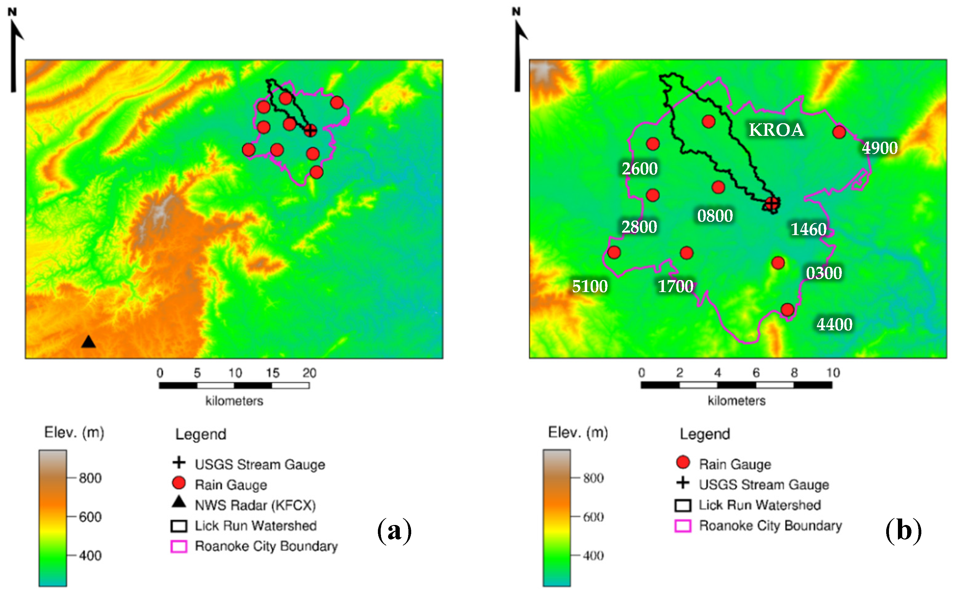
This study examines the Lick Run watershed (~19.4 km2), a tributary of the Roanoke River located in Roanoke, Virginia, U.S. (Figure 1). The watershed is approximately 35% impervious and subject to a variety of land uses [27]. Located in a mountain valley, the Roanoke-metropolitan area has a history of frequent flooding, resulting in property damage and sometimes death. Much of the basin is served by the city’s municipal separate storm sewer system (MS4). In the study area, the average distance between rain gauges is ~6.5 km, and the gauge density in the Lick Run basin is 1 gauge per 9.7 km2. A USGS stream gauge provides high accuracy, near real-time measurements of discharge at the basin’s outlet every five minutes.
2.2. QPE Datasets
Multiple agencies operate platforms with both real-time access to and long-term archives of rain gauge and other hydrometeorological data. Two of the most commonly-used networks in the U.S. are the National Water Information Service (NWIS) operated by the United States Geological Survey (USGS) and the Automated Surface Observation System (ASOS) operated jointly by the National Weather Service (NWS), the Department of Defense (DOD), and the Federal Aviation Administration (FAA). In Roanoke, Virginia, the USGS recently installed a network of nine rain gauges that provide fairly good coverage of the metropolitan area. These gauges became operational at the beginning of March 2018. The ASOS gauge (ID: KROA) located at the Roanoke airport has an archive going back to 1948. Full gauge identifiers and corresponding abbreviations are shown in Table A1. Gauge data were used to create three of the four QPE datasets: rainfall fields derived by kriging 5-min incremental depths measured at all 10 rain gauges, MFB-corrected 5-min incremental depths, and a basin-uniform estimate based on the measured 5-min depth at the KROA gauge. Level III instantaneous precipitation rates from the KFCX radar near Roanoke were used to create two of the four QPE datasets: uncorrected 5-min incremental depths and MFB-corrected 5-min depths.
2.3. QPE Processing
Among gauge-based estimates, there is a variety of methods for spatial interpolation between gauges. Two such methods—ordinary kriging and inverse distance weighting—have generally been shown to yield the most accurate rainfall estimates [28,29]. Kriging is a sophisticated method of spatial interpolation and generally performs well in areas where orographic effects on rainfall are present. Kriging involves creation of a variogram, or the relationship between distance and variance between points in a topological dataset, which is then used to estimate values between points.
Mean field bias (MFB) correction is perhaps the most common and easiest method for bias correction of radar rainfall data. MFB correction involves calculation of the ratio of average rainfall depth measured by selected gauges to the average depth determined by radar at the gauge location(s) (Equation (1)).
where:
- mean field bias
- precipitation depth at gauge i measured by the rain gauge (mm)
- precipitation depth at gauge i measured by uncorrected radar (mm)
- number of gauges
The MFB ratio can be calculated on any time scale (e.g., 1 day, 1 h, 5-min), using incremental depth measurements of the selected time scale. Once calculated, the ratios are applied to the entire uncorrected radar rainfall field at each time step (Equation (2)).
where:
- corrected radar rainfall depth field at time t (mm)
- uncorrected radar rainfall depth field at time t (mm)
- MFB ratio at time t
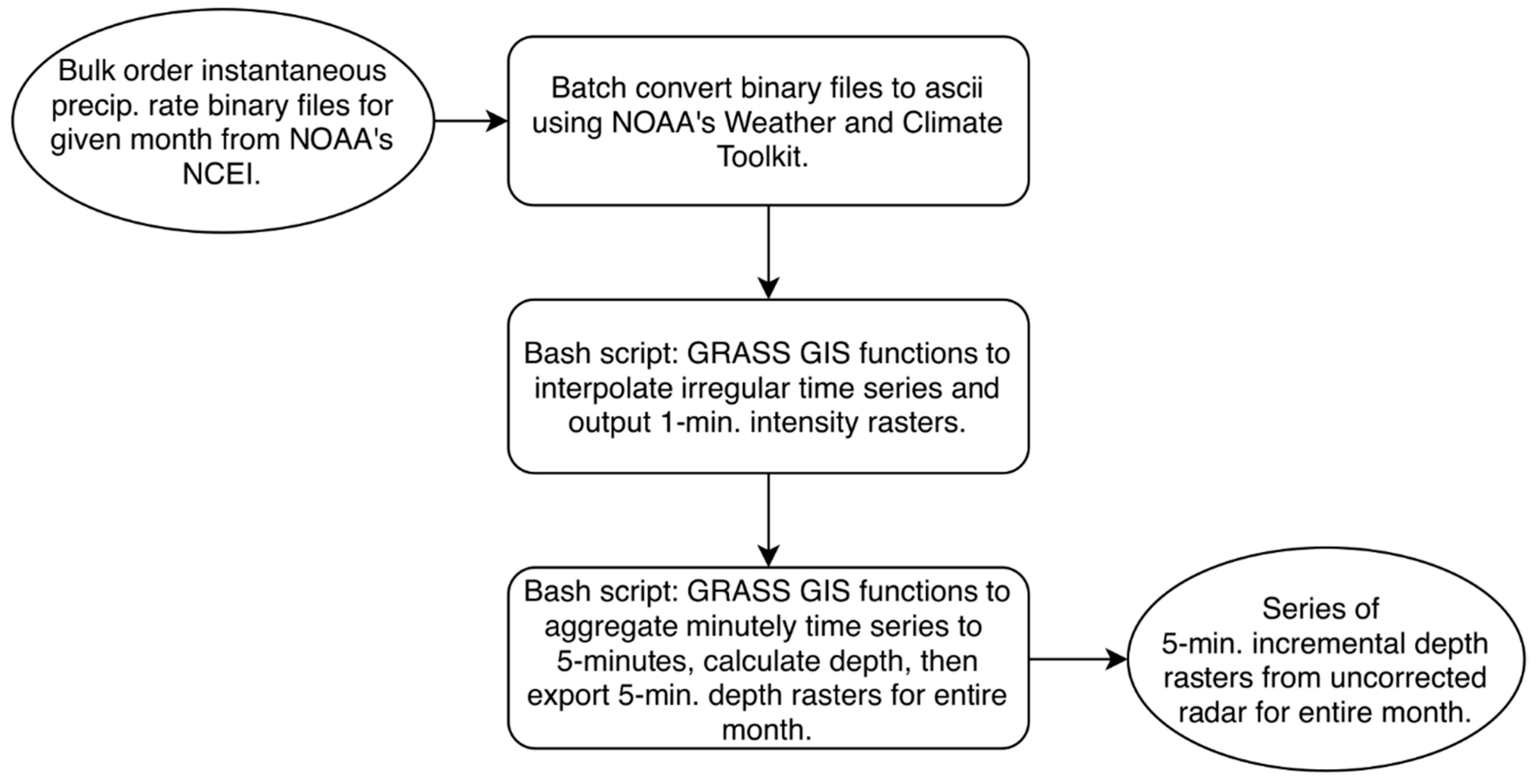
For this study, the mean field bias correction process involved correction of the Level III NEXRAD data using the 10 rain gauges in the study area. First, using Linux bash scripting and GRASS GIS 7.4 [30], the irregular time series of Level III instantaneous intensity raster grids were interpolated to a 1-min resolution. These 1-min intensity rasters were then used to calculate 5-min depth rasters, resulting in the uncorrected radar QPE (Figure 2).
Gauge precipitation data from NWIS and ASOS were retrieved and processed in R [31] to create a corresponding time series of 5-min incremental depths (Figure 3, Figure 4 and Figure 5). Over the 6-month study period, each NWIS gauge was typically missing slightly less than two days of data in total or ~1% of the entire period (Table A2). For each NWIS gauge, R was used to create a placeholder data frame with a 5-min time step that covered the entire study period. A separate data frame that held the downloaded NWIS gauge data and had missing data periods was joined to the placeholder data frame; any null values (missing data) in the resulting data frame were replaced with zero values. Missing data were not observed for the KROA gauge. However, since the KROA gauge had an irregular time series (typically a 5-min resolution, but not consistently), the incremental depths were temporally interpolated to a 1-min resolution, then aggregated to a 5-min resolution. Any missing data periods would be filled during the interpolation process. Similarly, since the Level III DPR radar data also had an irregular time series, any missing data periods would be filled during the temporal interpolation process.
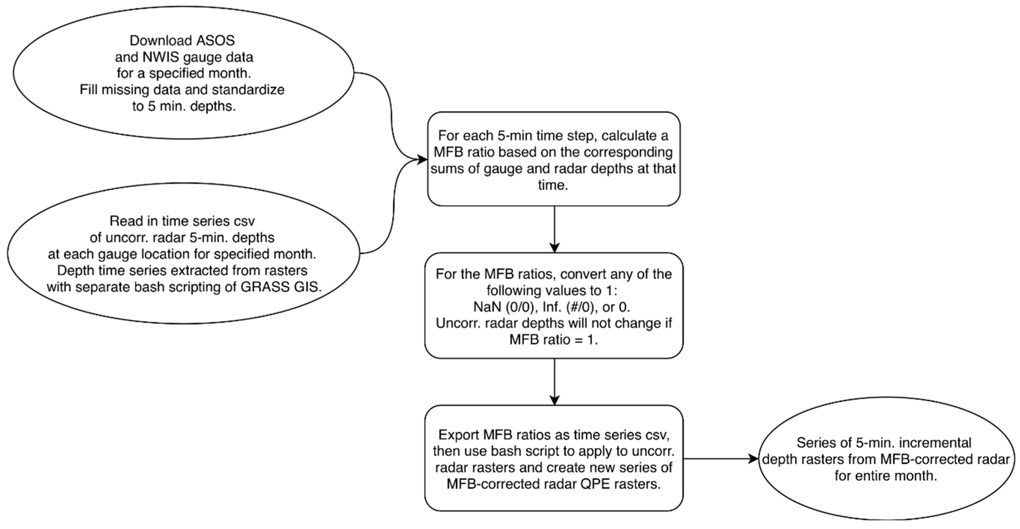
For MFB correction, a sample of the uncorrected radar (uncorr.) estimated precipitation depth was taken every five minutes at each gauge location for the study period. MFB ratios were calculated every five minutes from the sampled radar depths and gauge depths. MFB ratios of infinity (Inf.), “not a number” (NaN), or 0 (resulting from #/0, 0/0, or 0/#, respectively) were replaced with 1. The MFB ratios were then applied to the archive of 5-min, uncorrected radar rainfall fields, creating a new set of corrected rainfall fields (Figure 3). A final bash script was used to re-project the rasters spatially to the Hydrologic Rainfall Analysis Project (HRAP) projection [32] and convert the ASCII radar grids to XMRG files prior to model input. XMRG is a binary file format commonly used by NWS and required for RDHM input [33].
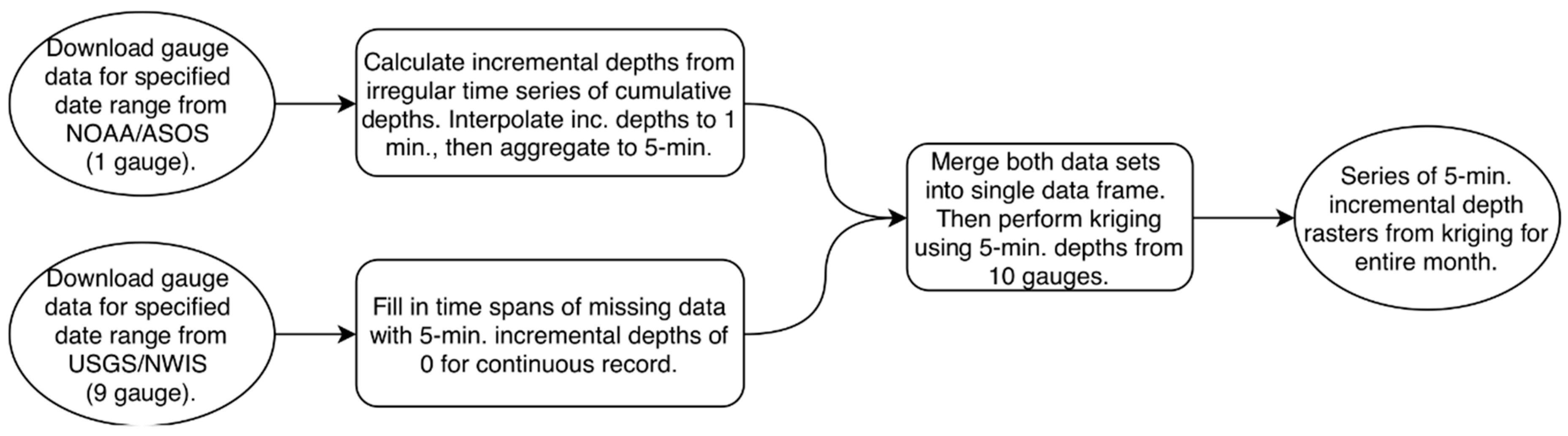
The 5-min incremental (inc.) gauge data were spatially interpolated by kriging using the autoKrige function in the automap R library [34]. autoKrige automatically determines which model to use for variogram fitting (e.g., spherical, Gaussian, exponential) based on the given point data, then uses the resulting variogram to perform kriging. The resulting rainfall fields were then reprojected to HRAP and converted to XMRG files (Figure 4).
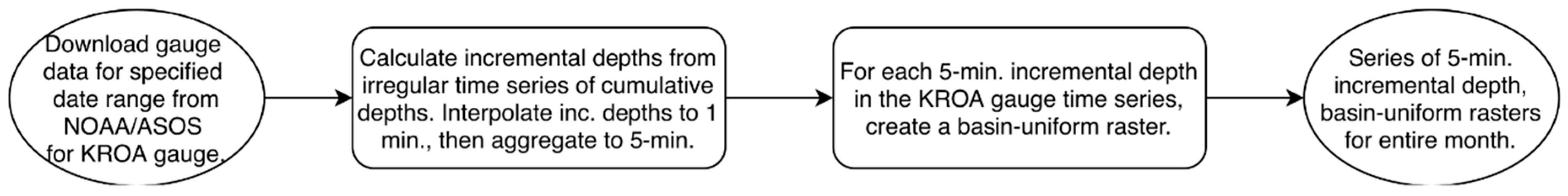
Creation of the single-gauge, uniform-basin QPE simply involved using the 5-min incremental depths from the KROA gauge time series to create a series of rasters populated with the gauge depth at each time step (Figure 5).
All of the QPE products were created at a resolution of 600 m to match the native resolution of the original Level III radar data, but were later re-sampled to 300 m before RDHM input to match the model resolution. In total, an archive of high-resolution data was created for the four QPE products (kriging, MFB corrected radar, uncorrected radar, and single gauge) spanning from 1 May 2018–31 October 2018, a period during which approximately two-thirds of the total annual precipitation occurred.
2.4. Research Distributed Hydrologic Model
The National Weather Service (NWS) Hydrology Laboratory previously developed a distributed H&H model called the Research Distributed Hydrologic Model (RDHM), which is one of the models used for hydrologic forecasting in various NWS River Forecasting Centers (RFCs). Principal model components include Sacramento-Soil Moisture Accounting (SAC-SMA), rutpix overland and channel routing (kinematic wave), and SNOW-17 for snow operations. RDHM comes with a set of a priori SAC-SMA parameters that have been developed for the entire conterminous United States (CONUS) and were derived using soil and land cover data from the Soil Survey Geographic Database (SSURGO) and National Land Cover Dataset (NLCD), respectively. Similarly, a CONUS-wide set of rutpix parameters is provided based on elevation data originally at a 400-m resolution [26]. However, the parameters, forcings, and resolution are typically derived and operated at a coarse scale, most commonly a 1 HRAP grid (nominally ~4 km). Model initialization is generally recommended and typically involves a 1-year or more warm-up simulation to determine initial model states for the study period. Calibration is also recommended, but is not possible in ungauged watersheds. The a priori parameters are therefore a useful tool for modeling in ungauged watersheds and aid in the calibration process for gauged watersheds [35].
For this study, a warm up simulation was run from 1 January 2017–31 December 2018 using precipitation and 2-m air temperature data from NASA’s Land Data Assimilation Systems (NLDAS). NLDAS provides real-time and historic land surface states, surface water fluxes, and energy fluxes at an hourly, 1/8-degree resolution. NLDAS variables originate from station-, remote-, and model-based data. The NLDAS precipitation data used in this study were derived from parameter-elevation regressions on independent slopes model (PRISM) adjusted daily gauge measurements resampled to an hourly scale using NEXRAD Stage II radar data. Most of the atmospheric variables in NLDAS, 2-m air temperature included, come from the North American Regional Reanalysis (NARR) [36]. From this historical simulation, the model states (e.g., channel depth, flow rate, soil water content, etc.) at the beginning of each month were used as the initial states for each monthly simulation (May–November 2018) forced with the high-resolution QPE datasets. RDHM was operated at a 1/16 HRAP grid resolution (approximately 300 m) due to the small size of the watershed and was run uncalibrated to avoid introducing bias towards one of the QPE methods. Simulated discharge at the basin’s outlet from each of the precipitation forcings was compared to observed discharge measured by the USGS stream gauge.
Although gridded estimates of other hydrologic variables were generated from the RDHM simulations, including soil moisture, surface/subsurface flow, soil temperature, etc., these variables were not evaluated. This is due to the lack of observed data at the needed spatiotemporal resolution for meaningful comparisons. Furthermore, the study’s emphasis was on hydrologic prediction for flood monitoring in small urban watersheds, not a detailed evaluation of the RDHM.
3. Results
3.1. QPE Products
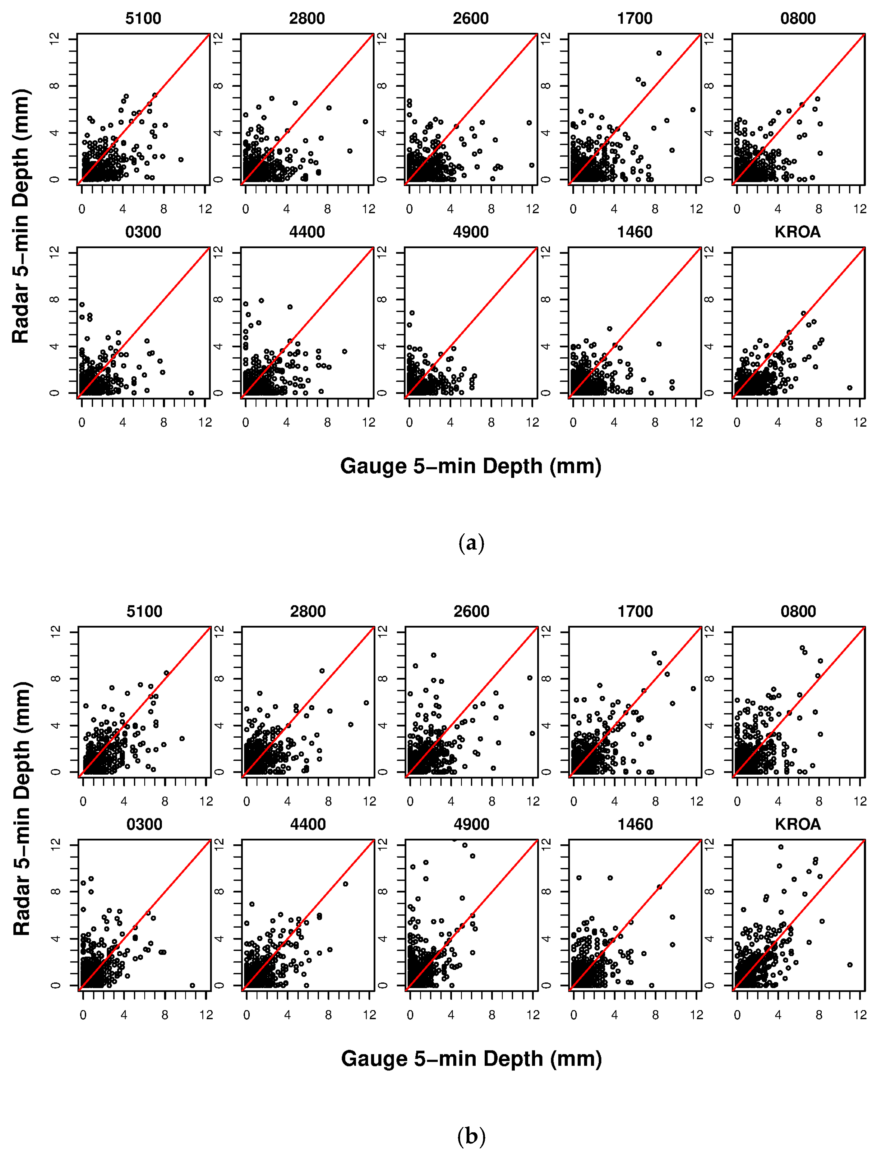
Multiple QPE products were generated at a 5-min, 600-m resolution for model input, including: uncorrected Level III radar data, MFB-corrected Level III radar data, kriged rain gauge data (10 gauges), and a watershed uniform depth based on measurements at the KROA rain gauge. Figure 6 shows a comparison of gauge and radar 5-min incremental depths before (a) and after (b) MFB correction. MFB correction appears to result in overestimation for the upper range of corrected radar rainfall depths (Figure 6b), resulting in overestimation of predicted discharge for simulations forced with MFB-corrected radar data.
From the 5-min incremental depths, cumulative depths were calculated over the study period for gauge, uncorrected radar, and MFB corrected radar QPEs at each gauge location (Figure 7).
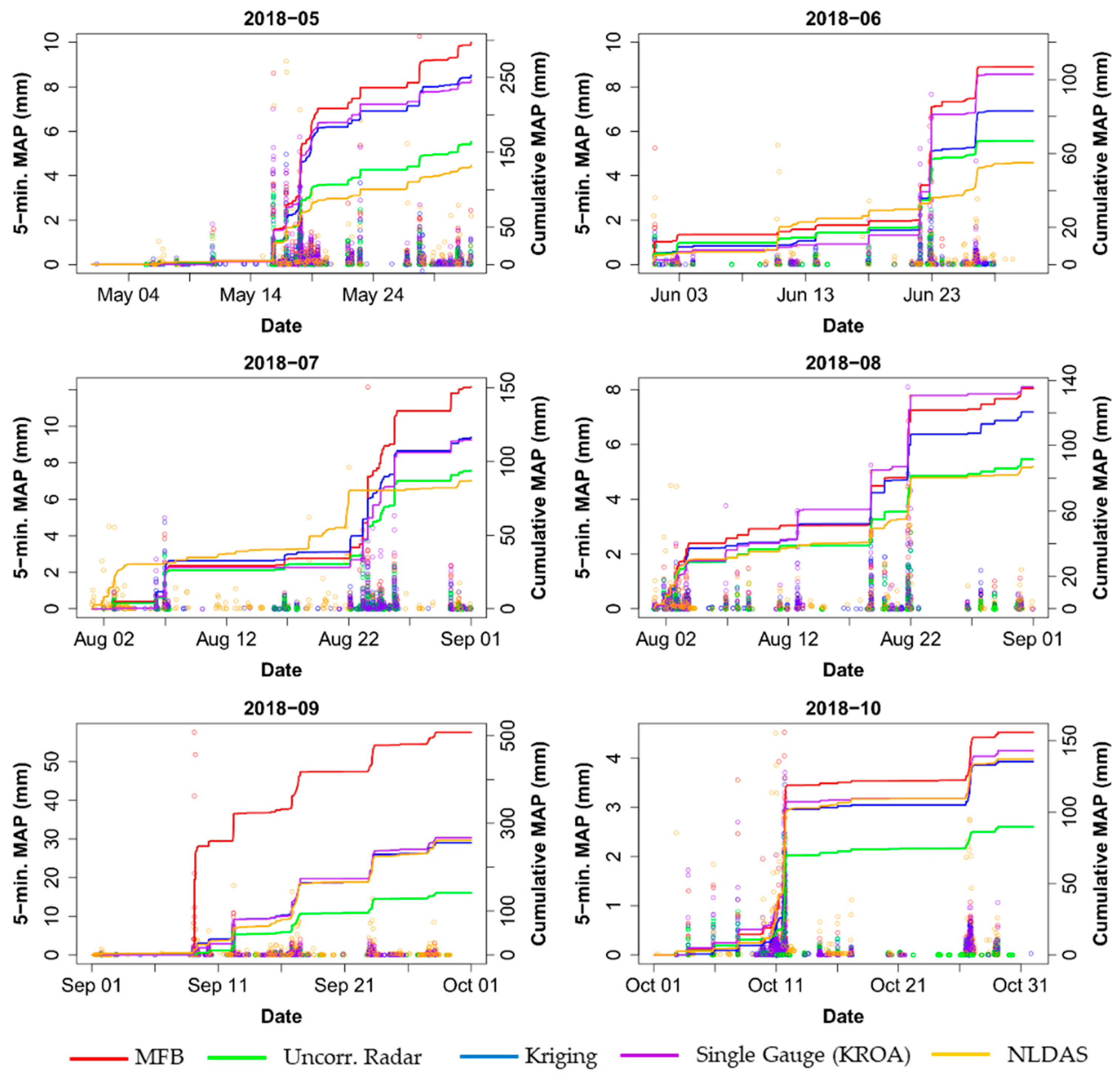
Mean areal precipitation (MAP) over the Lick Run basin was calculated by RDHM during each simulation along with the discharge time series. From the incremental MAP, the cumulative MAP was calculated for each month (Figure 8).
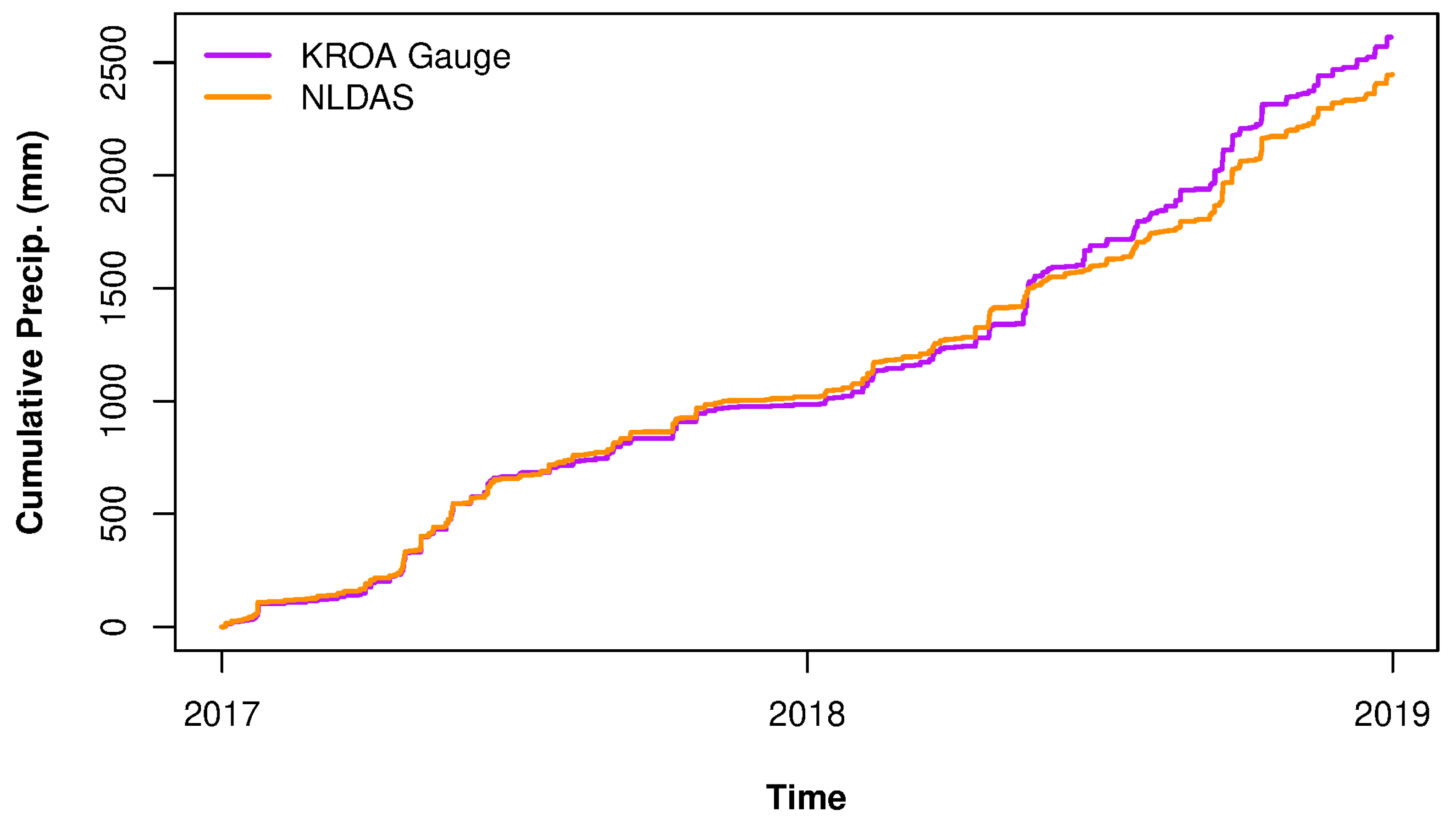
In order to evaluate discharge overprediction by certain high-resolution QPE methods (e.g., MFB correction and kriging), the cumulative MAP from NLDAS and the KROA gauge between the beginning of 2017 and the end of 2018 was calculated and compared (Figure 9). The cumulative MAP from KROA and NLDAS was 2612 mm and 2447 mm, respectively; a difference of 165 mm.
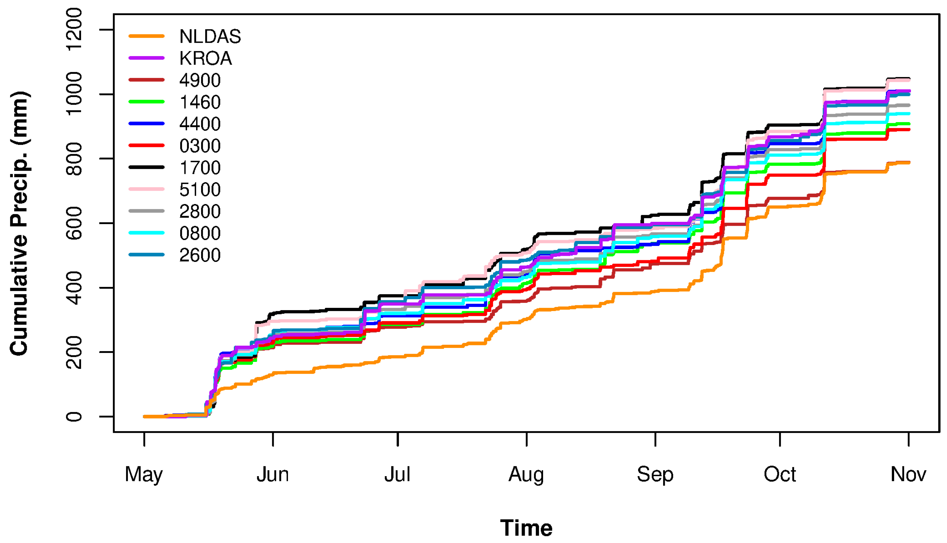
For the six-month study period in 2018, cumulative precipitation between NLDAS and each gauge in the network was calculated and compared (Figure 10). NLDAS had the lowest cumulative depths over the study period and appeared to underpredict for larger storm events. Note that the final difference in cumulative precipitation between the KROA gauge and NLDAS is different in Figure 9 and Figure 10. This was due to the different time frames over which cumulative precipitation was calculated and was exaggerated due to differing y-axis scales.
3.2. Model Results
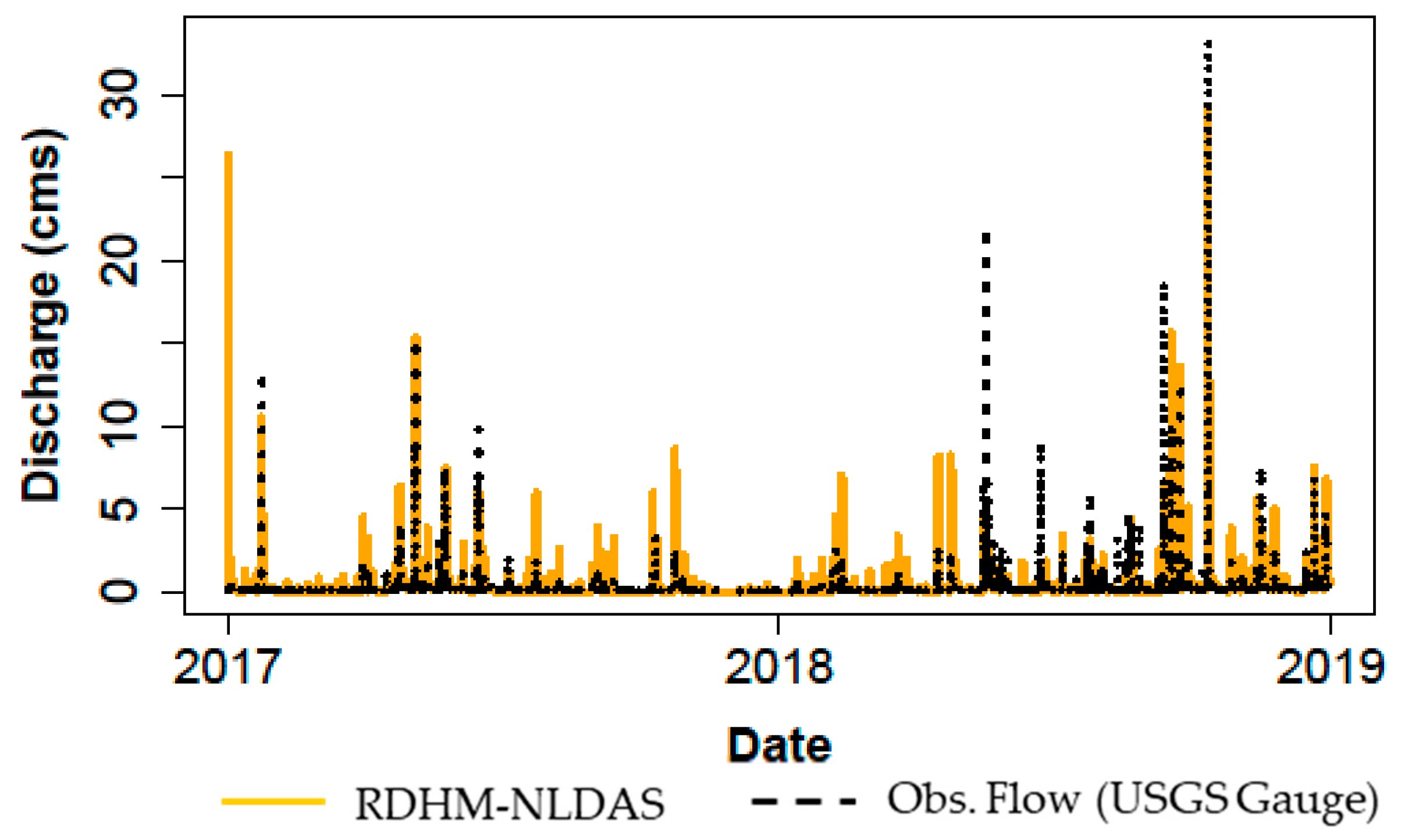
From the uncalibrated historical simulation, a time series of predicted discharge at the basin outlet was generated by RDHM, then compared with USGS stream gauge measurements at the same location (Figure 11).
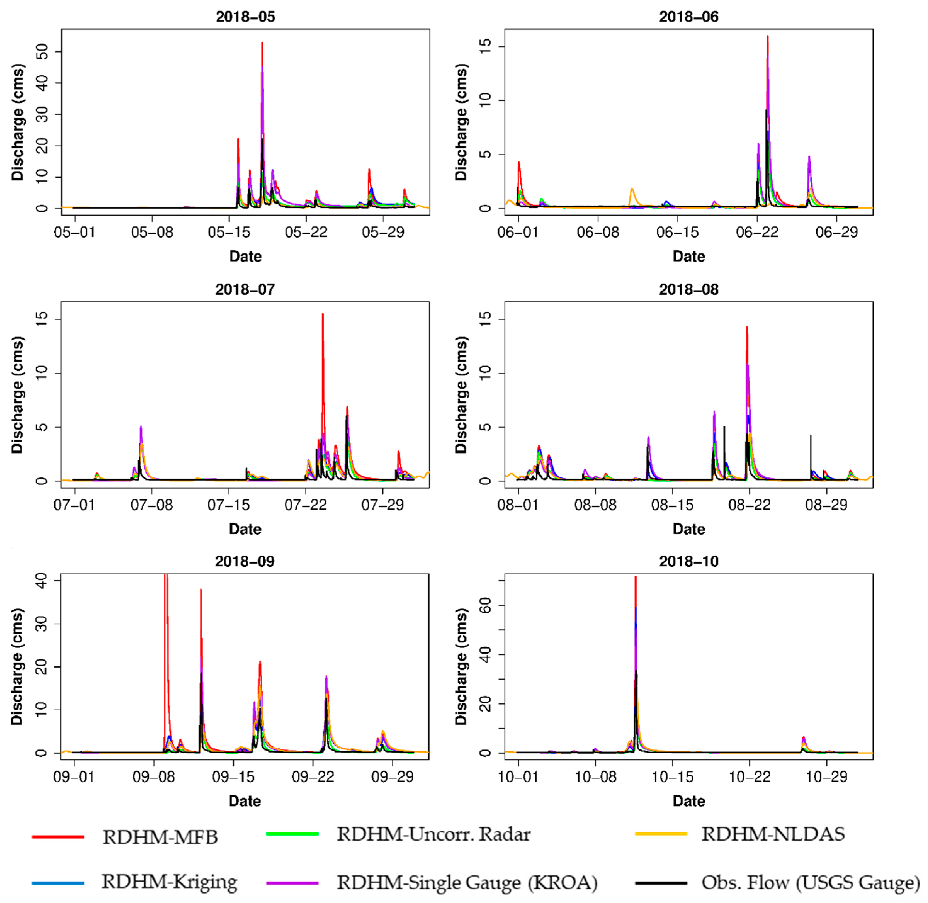
The saved model states from this historical simulation were used as warm start values for the monthly simulations forced with each of the four high-resolution QPEs (Figure 12).
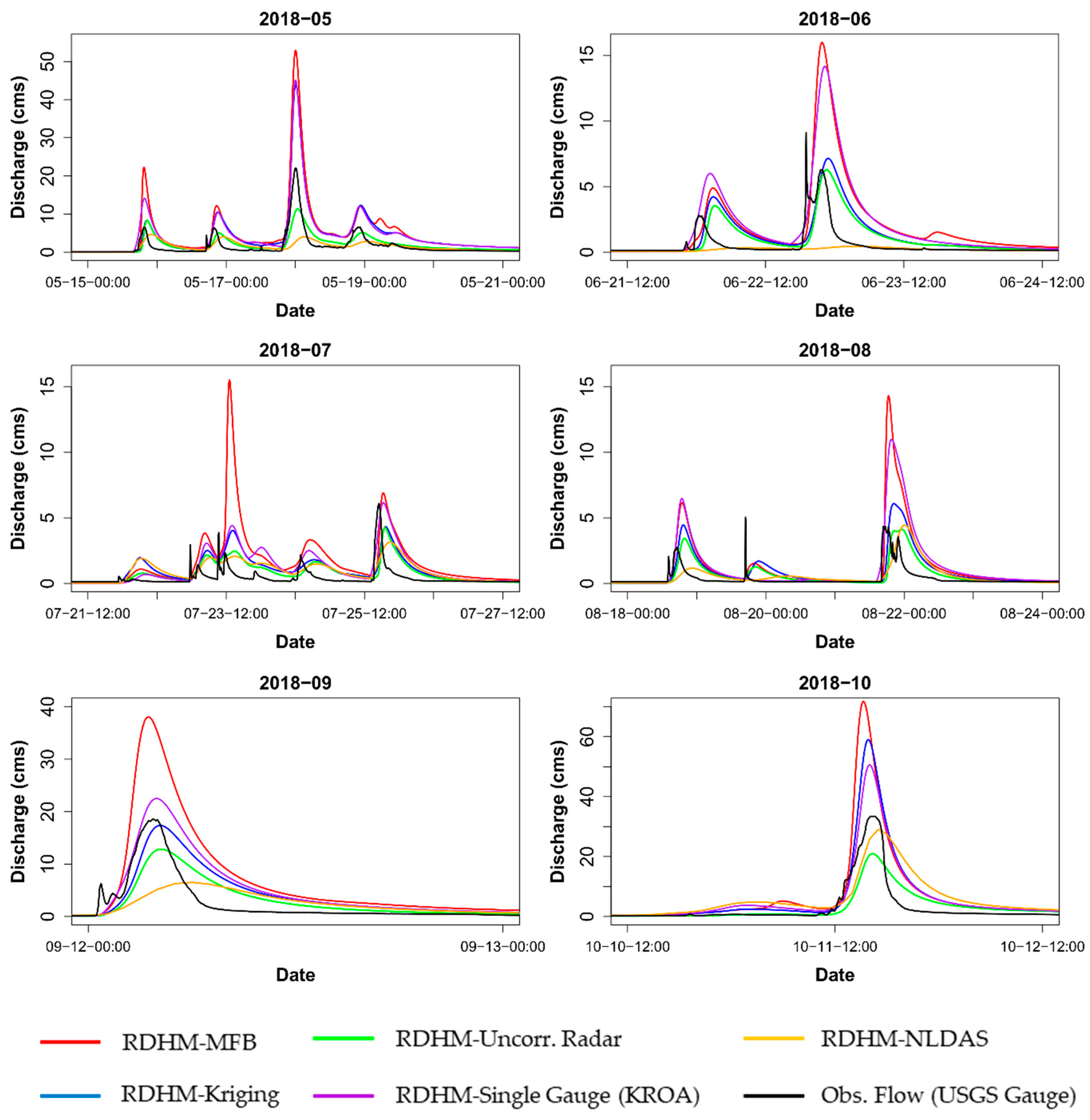
Figure 13 shows the largest flow events from each month of the high-resolution simulations.
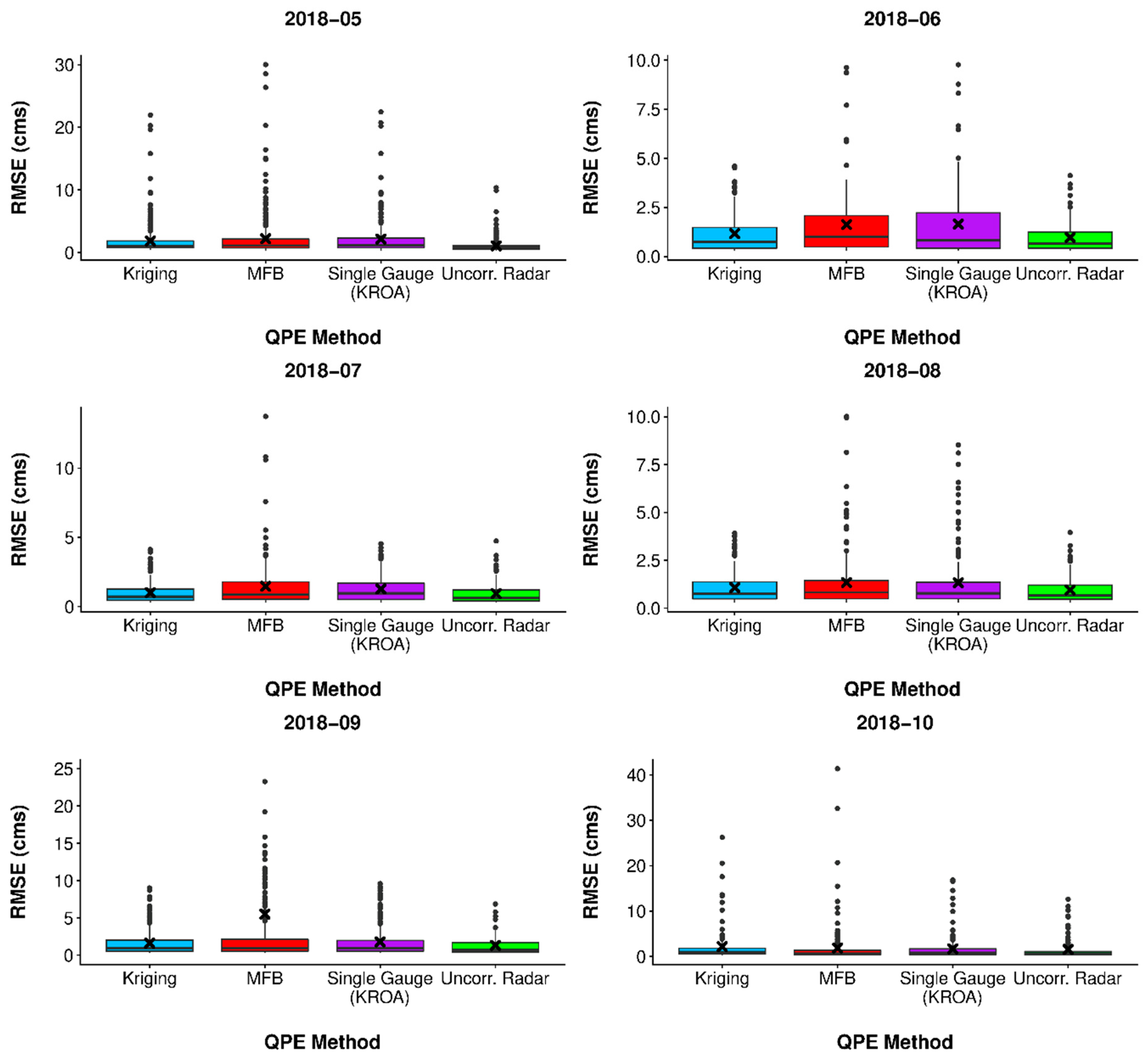
Since the monthly simulations were conducted on a continuous basis, the root mean squared error (RMSE) was calculated hourly rather than on an event basis. Similarly, RMSE values calculated during baseflow periods were removed. Here, baseflow was defined as anything less than 0.3 cubic meters per second (cms), and any hourly RMSE values less than 0.3 cms were removed. Figure 14 shows the hourly RMSE values for each QPE forcing by month.
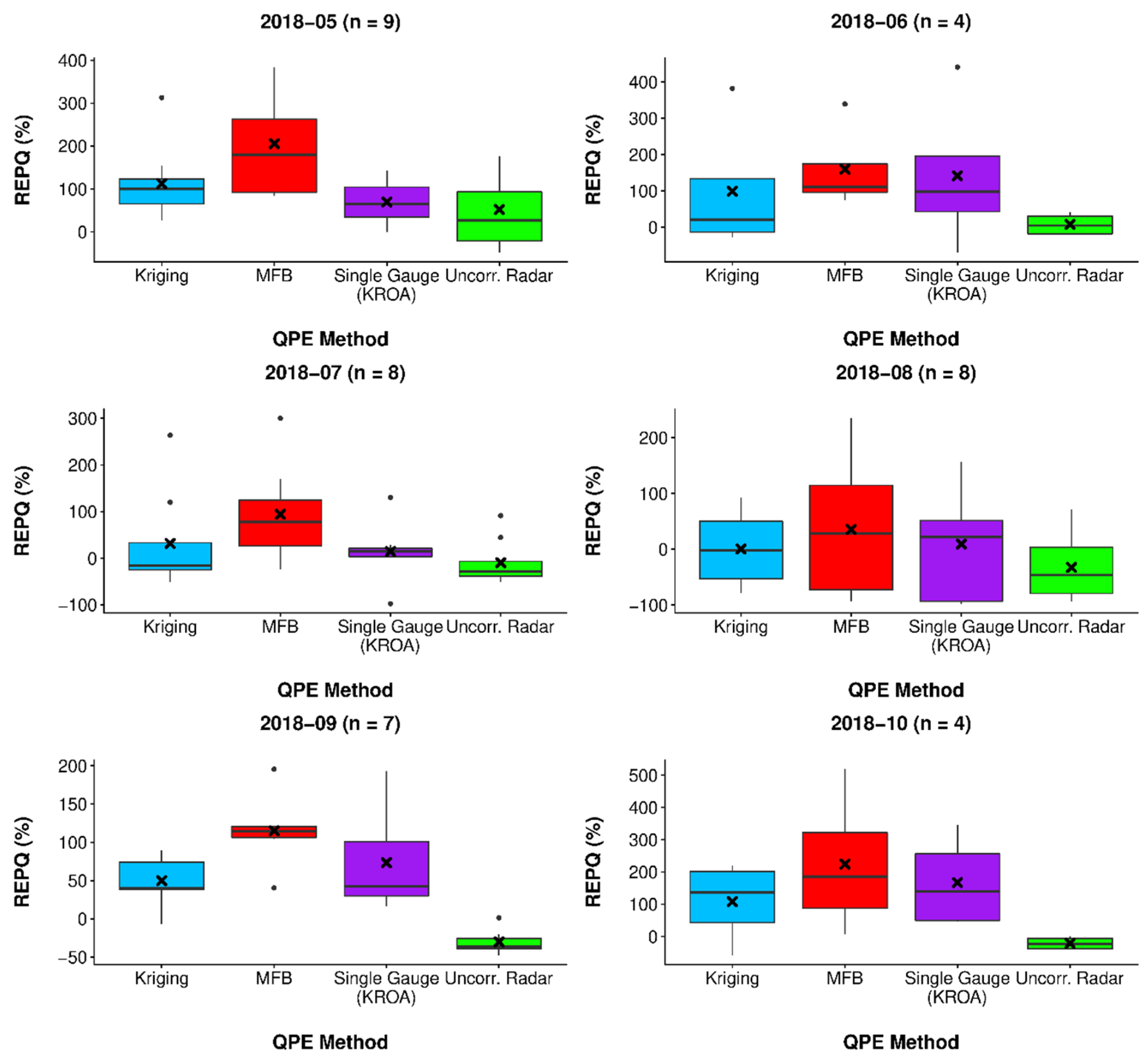
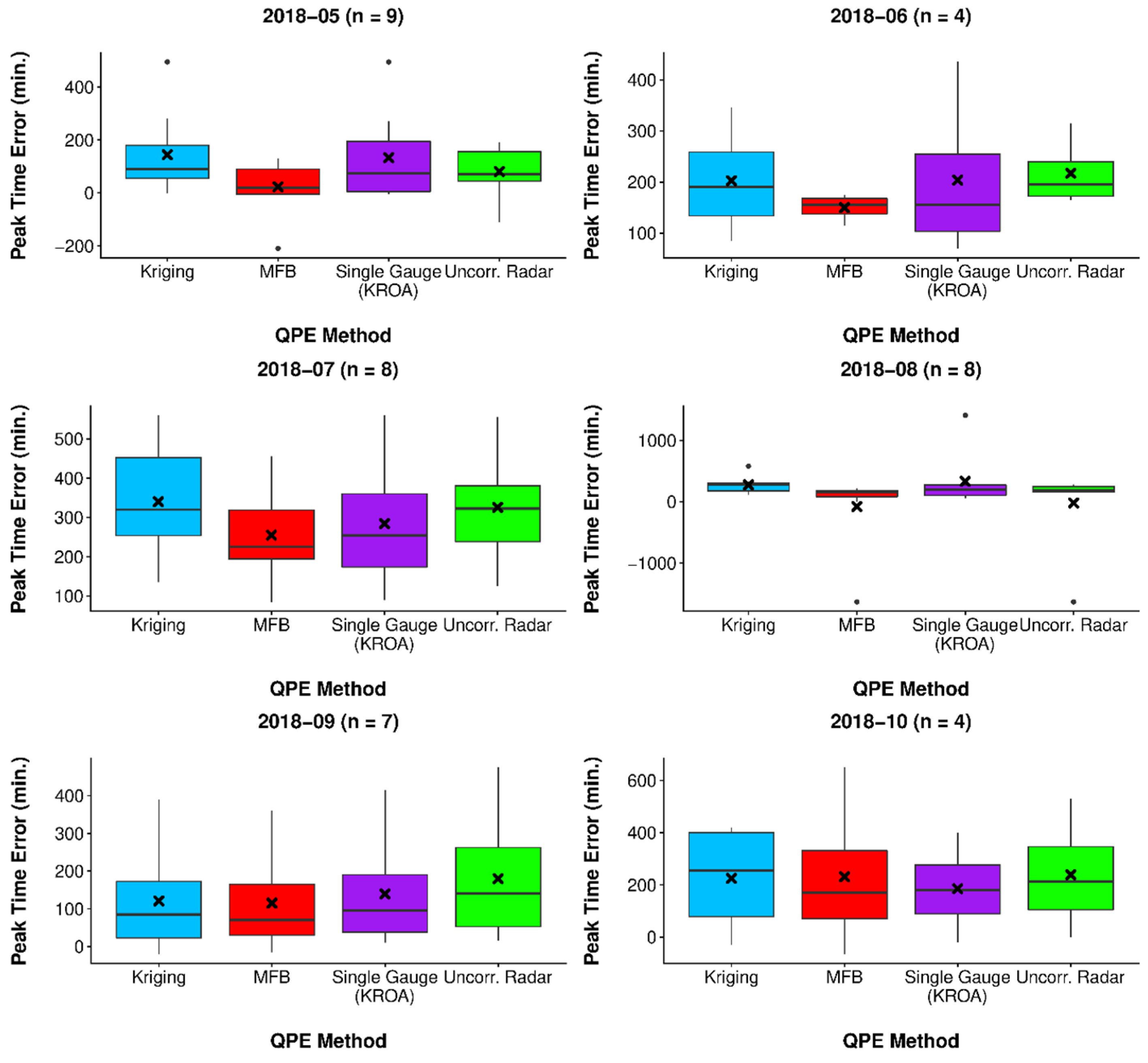
Relative error in peak flow (REPQ) was analyzed by QPE forcing for each month by extracting the peaks for any flow event that surpassed 1 cms (Figure 15). The peak time error (PTE) for these events was also summarized (Figure 16). The number of flow events analyzed each month (n) ranged from 4–9.
Forty (40) flow events above 1 cms occurred between 1 May 2018 and 1 November 2018. A summary of RMSE, REPQ, and PTE is shown in Table 1.
4. Discussion
The RDHM simulations yielded interesting and counterintuitive results: the uncorrected radar QPE forcing resulted in the most accurate discharge predictions, rather than the more sophisticated methods of kriging and MFB correction. Regarding predicted discharge magnitude, the simulations forced with uncorrected radar data had the lowest error as measured by hourly RMSE and peak flow relative error. The kriging and single-gauge QPE forcings resulted in moderately worse and relatively similar performance statistics; while the MFB-corrected radar QPE led to significantly worse results, caused by severe and consistent overprediction. In terms of peak timing, the MFB forcing performed moderately better than the remaining QPE methods, all of which had similar aggregate results.
As expected, the uncorrected radar systematically underpredicted. Less expected was the overprediction of the three other QPE forcings (MFB, kriging, single gauge). There are several possible explanations for the overestimation of the three QPE forcings: model parameterization, QPE methodology, and/or model initialization.
Here, model parameterization refers to the a priori SAC-SMA and rutpix routing parameters based on soil, land cover, and elevation data. Potentially, the resolution of the datasets from which the parameters were derived and/or the resolution of the resulting parameter grids (one HRAP grid resolution) was too coarse for small, urban watersheds. Alternatively, mechanisms in the parameter derivation process led to parameters which caused overestimated discharge predictions. One or both of these rationales would explain the performance statistics of the uncorrected radar: even though radar data that have not been gauge corrected are well known to unpredict precipitation, discharge overestimation attributed to RDHM parameterization may increase the predicted flow such that the uncorrected radar forcing had the highest skill. Re-derivation of model parameters using higher resolution data and/or producing higher resolution parameter grids may mitigate this overestimation.
Besides model parameterization, another potential source of overestimation is the QPE methodology used to create the various precipitation forcings. Potentially, even a gauge density of ~6.5 km is too coarse for small, urban watersheds. Similarly, single-gauge coverage for a ~19.4 km2 watershed appears to be inadequate. Both of these possibilities would support prior studies’ recommendations of QPE resolution on the order of 1 km [20,21,22,23].
There are several potential sources of error for the MFB-corrected QPE. One possibility is random error associated with the MFB correction process. Much of the systematic bias was removed during the MFB process, but significant random error persisted, likely due to the small time scale (5-min) of the correction process (Figure 6). This supports prior findings [20,37] that a longer time scale is needed for MFB correction to remove random errors, but the time scale cannot be so long such that the drop size distribution (DSD) changes. Changes in DSD are a particular concern for short, intense convective storms common during summer months, where storm durations are likely to be sub-hourly and DSD can change over the course of several minutes. Further, while the MFB process provided relatively good correction of the radar data at each gauge location (Figure 7), precipitation overprediction may have resulted from spatial variability in field bias between gauges. This suggests that even at small spatial scales, using the mean of the field bias does not provide adequate correction, necessitating a spatially-varied correction method. One example of this occurred in early September 2018: gauge and radar depths inside the watershed were zero or negligible, but moderate, and trace depths for gauge and radar estimates, respectively, at gauge location(s) outside the watershed resulted in very high MFB ratios, such that the MAP inside the basin was erroneously and highly inflated. This phenomenon can be seen in the several high incremental MFB MAP values during September 2018 in Figure 8 and the resulting impact on predicted discharge, as well as cumulative MAP. This also suggests that an outlier threshold is required for MFB correction.
A third possible source of overestimation may be the saved model states from the historical simulation that were used as warm start values for the monthly simulations. The coarse resolution of the NLDAS forcings (13.5-km, 1-h) may not be adequate for estimating model states (e.g., soil moisture) in small, urban watersheds. Similarly, a finer model resolution (e.g., 30 m instead of 300 m) may improve performance at the cost of increased model run time.
Generally, the MAP from the MFB QPE was consistently higher than the remaining QPE methods and except for one or two exceptions was relatively close to the MAP from the kriging and single-gauge QPEs. Conversely, the MAP from the uncorrected radar was consistently and significantly the lowest of the four high-resolution QPEs. For three of six months, NLDAS had the lowest cumulative MAP, but for the other three months, it had cumulative MAP similar to the kriging and single-gauge QPEs. The cumulative MAP from NLDAS and the KROA gauge between 1 January 2017 and 1 January 2019 tracked closely, with a final difference of 165 mm. As an operational dataset, NLDAS is a reliable QPE on hourly and daily time scales, which seems to confirm both the accuracy of the KROA gauge (Figure 9) and the overprediction of the MFB-corrected QPE. However, it does appear that NLDAS underpredicts as storm total precipitation depth increases (e.g., first rainfall event in Figure 10).
Several other findings regarding QPE temporal resolution, gauge density, and model calibration can be posited from the study. Although overall cumulative MAP between NLDAS and several of the high-resolution QPEs was similar, consistent underprediction of discharge when forced with NLDAS suggests that hourly precipitation inputs are inadequate for modeling small, urban watersheds, a finding echoed by prior research [20,21,22,23]. Similar results from the kriging and single-gauge QPEs indicate that, for the gauge density and basin size of this study (one gauge per 9.7 km2 and 19.4 km2, respectively), a single-gauge QPE (using a gauge inside the watershed) can provide results on-par with estimates from kriging. While these two QPE products at the given density were not optimal for RDHM, better performance may be achieved with other models. Calibration would improve model skill; however, calibration would necessarily bias model results towards the QPE forcing used in calibration, making comparisons between different QPE forcings tenuous.
The RDHM was not calibrated, so fast response hydrograph features were not captured well (e.g., Figure 13, second flow event in the 2018-06 series). Additionally, the model does not have the capability to model storm sewer infrastructure and does not account for detailed variations in channel cross-section geometry. However, with better parameterization, calibration, and possibly a higher model resolution, RDHM has the potential to predict peaks and volume skillfully, even in small, urban watersheds. The relatively good performance of the uncorrected radar QPE with RDHM makes this pairing an attractive option for high-resolution discharge simulations in small, gauged or ungauged watersheds; especially considering that both the Level III dataset and the RDHM parameters have coverage for the entire CONUS.
5. Conclusions
Overall, this study examined various QPE methods for continuous, distributed hydrological modeling in a small urban watershed using an operational H&H model. Of the four high-resolution precipitation forcings used, the uncorrected Level III radar QPE resulted in the most accurate discharge predictions from RDHM. This suggests that when paired with RDHM, the Level III dataset has the potential for use in hydrologic modeling of small, urban watersheds, even without bias correction. Model calibration is recommended.
Future studies that use RDHM in small urban watersheds should compare various parameter and model resolutions, as well as uncalibrated versus calibrated simulations. Similarly, the effect of outlier removal on MFB QPE simulation skill should be examined. Finally, more advanced bias correction algorithms, such as those used in the Multi-Radar Multi-Sensor (MRMS) system [38], are needed at finer spatial and temporal resolutions.
Author Contributions
D.W. contributed to experimentation, analysis, writing, and editing. T.E.A.I. contributed to contributed to experimentation, analysis, and revisions. R.D. contributed to project administration, funding acquisition, and revisions.
Funding
This research received no external funding.
Conflicts of Interest
The authors declare no conflict of interest.
Appendix A
Table A1 shows the full rain gauge identifier (ID) for each of the abbreviated IDs used in various graphics.

Table A1.
Full and abbreviated rain gauge IDs.
| Full ID | Abbreviated ID |
|---|---|
| 371840079534900 | 4900 |
| 205551460 | 1460 |
| 371339079554400 | 4400 |
| 371459079560300 | 0300 |
| 371518079591700 | 1700 |
| 371520080015100 | 5100 |
| 371657080002800 | 2800 |
| 371709079580800 | 0800 |
| 371824080002600 | 2600 |
| KROA | KROA |
Table A2 shows the missing data periods for each of the NWIS gauges.
Table A2.
Missing data periods by gauge ID.
| Gauge ID | # of Missing 5-min Periods | Total Missing Time (hours) | Missing Observations as % of Total Observations |
|---|---|---|---|
| 0205551460 | 565 | 47.08 | 1.07% |
| 371339079554400 | 558 | 46.50 | 1.05% |
| 371459079560300 | 161 | 13.42 | 0.30% |
| 371518079591700 | 570 | 47.50 | 1.08% |
| 371520080015100 | 560 | 46.67 | 1.06% |
| 371657080002800 | 562 | 46.83 | 1.06% |
| 371709079580800 | 559 | 46.58 | 1.05% |
| 371824080002600 | 558 | 46.50 | 1.05% |
| 371840079534900 | 559 | 46.58 | 1.05% |
References
- Fonstad, M.A.; Dietrich, J.T.; Courville, B.C.; Jensen, J.L.; Carbonneau, P.E. Topographic structure from motion: A new development in photogrammetric measurement. Earth Surf. Process. Landf. 2013, 38, 421–430. [Google Scholar] [CrossRef]
- Mayer, H. Automatic Object Extraction from Aerial Imagery—A Survey Focusing on Buildings. Comput. Vis. Image Underst. 1999, 74, 138–149. [Google Scholar] [CrossRef]
- Tokarczyk, P.; Leitao, J.P.; Rieckermann, J.; Schindler, K.; Blumensaat, F. High-quality observation of surface imperviousness for urban runoff modelling using UAV imagery. Hydrol. Earth Syst. Sci. 2015, 19, 4215–4228. [Google Scholar] [CrossRef] [Green Version]
- Gironás, J.; Niemann, J.D.; Roesner, L.A.; Rodriguez, F.; Andrieu, H. Evaluation of methods for representing urban terrain in stormwater modeling. J. Hydrol. Eng. 2010, 15, 1–14. [Google Scholar] [CrossRef]
- Smith, B.K.; Smith, J.A.; Baeck, M.L.; Villarini, G.; Wright, D.B. Spectrum of storm event hydrologic response in urban watersheds. Water Resour. Res. 2013, 49, 2649–2663. [Google Scholar] [CrossRef]
- Cristiano, E.; ten Veldhius, M.-C.; van de Giesen, N. Spatial and temporal variability of rainfall and their effects on hydrological response in urban areas—A review. Hydrol. Earth Syst. Sci. 2017, 21, 3859–3878. [Google Scholar] [CrossRef]
- Wang, L.P.; Ochoa-Rodríguez, S.; Van Assel, J.; Pina, R.D.; Pessemier, M.; Kroll, S.; Willems, P.; Onof, C. Enhancement of radar rainfall estimates for urban hydrology through optical flow temporal interpolation and Bayesian gauge-based adjustment. J. Hydrol. 2015, 531, 408–426. [Google Scholar] [CrossRef] [Green Version]
- Daniels, E.E.; Lenderink, G.; Hutjes, R.W.A.; Holtslag, A.A.M. Observed urban effects on precipitation along the Dutch West coast. Int. J. Climatol. 2016, 36, 2111–2119. [Google Scholar] [CrossRef]
- Freitag, B.M.; Nair, U.S.; Niyogi, D. Urban Modification of Convection and Rainfall in Complex Terrain. Geophys. Res. Lett. 2018, 45, 2507–2515. [Google Scholar] [CrossRef]
- National Academies of Sciences, Engineering, and Medicine. Framing the Challenge of Urban Flooding in the United States; National Academies Press: Washington, DC, USA, 2019. [Google Scholar]
- Yoon, S.S.; Lee, B. Effects of using high-density rain gauge networks and weather radar data on urban hydrological analyses. Water 2017, 9, 931. [Google Scholar] [CrossRef]
- Krajewski, W.F.; Ciach, G.J.; Habib, E. An analysis of small-scale rainfall variability in different climatic regimes. Hydrol. Sci. J. 2003, 48, 151–162. [Google Scholar] [CrossRef] [Green Version]
- Ogden, F.L.; Sharif, H.O.; Senarath, S.U.S.; Smith, J.A.; Baeck, M.L.; Richardson, J.R. Hydrologic analysis of the Fort Collins, Colorado, flash flood of 1997. J. Hydrol. 2000, 228, 82–100. [Google Scholar] [CrossRef]
- James, W.P.; Robinson, C.G.; Bell, J.F. Radar-Assisted Real-Time Flood Forecasting. J. Water Resour. Plan. Manag. 1993, 119, 32–44. [Google Scholar] [CrossRef]
- Pessoa, M.L.; Bras, R.L.; Williams, E.R. Use of Weather Radar for Flood Forecasting in the Sieve River Basin: A Sensitivity Analysis. J. Appl. Meteorol. 1993, 32, 462–475. [Google Scholar] [CrossRef] [Green Version]
- Sun, X.; Mein, R.G.; Keenan, T.D.; Elliott, J.F. Flood estimation using radar and raingauge data. J. Hydrol. 2000, 239, 4–18. [Google Scholar] [CrossRef]
- Kim, B.S.; Kim, B.K.; Kim, H.S. Flood simulation using the gauge-adjusted radar rainfall and physics-based distributed hydrologic model. Hydrol. Process. 2008, 22, 4400–4414. [Google Scholar]
- Looper, J.P.; Vieux, B.E. An assessment of distributed flash flood forecasting accuracy using radar and rain gauge input for a physics-based distributed hydrologic model. J. Hydrol. 2012, 412, 114–132. [Google Scholar] [CrossRef]
- Seo, B.-C.; Krajewski, W.F.; Quintero, F.; ElSaadani, M.; Goska, R.; Cunha, L.K.; Dolan, B.; Wolff, D.B.; Smith, J.A.; Rutledge, S.A.; et al. Comprehensive Evaluation of the IFloodS Radar Rainfall Products for Hydrologic Applications. J. Hydrometeorol. 2018, 19, 1793–1813. [Google Scholar] [CrossRef]
- Thorndahl, S.; Einfalt, T.; Willems, P.; Ellerbæk Nielsen, J.; Ten Veldhuis, M.C.; Arnbjerg-Nielsen, K.; Rasmussen, M.R.; Molnar, P. Weather radar rainfall data in urban hydrology. Hydrol. Earth Syst. Sci. 2017, 21, 1359–1380. [Google Scholar] [CrossRef] [Green Version]
- Ochoa-Rodriguez, S.; Wang, L.P.; Gires, A.; Pina, R.D.; Reinoso-Rondinel, R.; Bruni, G.; Ichiba, A.; Gaitan, S.; Cristiano, E.; Van Assel, J.; et al. Impact of spatial and temporal resolution of rainfall inputs on urban hydrodynamic modelling outputs: A multi-catchment investigation. J. Hydrol. 2015, 531, 389–407. [Google Scholar] [CrossRef]
- Berne, A.; Delrieu, G.; Creutin, J.D.; Obled, C. Temporal and spatial resolution of rainfall measurements required for urban hydrology. J. Hydrol. 2004, 299, 166–179. [Google Scholar] [CrossRef]
- Schilling, W. Rainfall data for urban hydrology: What do we need? Atmos. Res. 1991, 27, 5–21. [Google Scholar] [CrossRef]
- Wang, L.P.; Ochoa-Rodriguez, S.; Onof, C.; Willems, P. Singularity-sensitive gauge-based radar rainfall adjustment methods for urban hydrological applications. Hydrol. Earth Syst. Sci. 2015, 12, 1855–1900. [Google Scholar] [CrossRef]
- Wang, L.P.; Ochoa-Rodríguez, S.; Simões, N.E.; Onof, C.; Maksimović, Č. Radar-raingauge data combination techniques: A revision and analysis of their suitability for urban hydrology. Water Sci. Technol. 2013, 68, 737–747. [Google Scholar] [CrossRef] [PubMed]
- Hydrology Laboratory-Research Distributed Hydrologic Model (HL-RDHM) User Manual V. 3.0.0. Available online: https://www.cbrfc.noaa.gov/present/rdhm/RDHM_3_0_0_User_Manual.pdf (accessed on 27 June 2019).
- Dymond, R.L.; Aguilar, M.F.; Bender, P.; Hodges, C.C. Lick Run Watershed Master Plan; Virginia Tech: Blacksburg, VA, USA, 2017. [Google Scholar]
- Chen, D.; Ou, T.; Gong, L.; Xu, C.Y.; Li, W.; Ho, C.H.; Qian, W. Spatial interpolation of daily precipitation in China: 1951-2005. Adv. Atmos. Sci. 2010, 27, 1221–1232. [Google Scholar] [CrossRef]
- Shope, C.L.; Maharjan, G.R. Modeling spatiotemporal precipitation: Effects of density, interpolation, and land use distribution. Adv. Meteorol. 2015, 2015, 1–16. [Google Scholar] [CrossRef]
- Geographic Resources Analysis Support System (GRASS) Software; GRASS Development Team: Bonn, Germany, 2018.
- R: A Language and Environment for Statistical Computing; R Core Team: Vienna, Austria, 2018.
- Fulton, R. WSR-88D Polar-to-HRAP Mapping; Hydrologic Research Laboratory Office of Hydrology National Weather Service: Silver Spring, MD, USA, 1998.
- National Weather Service. The XMRG File Format and Sample Codes to Read XMRG Files. Available online: https://www.nws.noaa.gov/ohd/hrl/dmip/2/xmrgformat.html (accessed on 15 April 2019).
- Hiemstra, P.H.; Pebesma, E.J.; Twenhöfel, C.J.W.; Heuvelink, G.B.M. Real-time automatic interpolation of ambient gamma dose rates from the Dutch radioactivity monitoring network. Comput. Geosci. 2009, 35, 1711–1721. [Google Scholar] [CrossRef]
- Zhang, Z.; Koren, V.; Reed, S.; Smith, M.; Zhang, Y.; Moreda, F.; Cosgrove, B. SAC-SMA a priori parameter differences and their impact on distributed hydrologic model simulations. J. Hydrol. 2012, 420, 216–227. [Google Scholar] [CrossRef]
- Xia, Y.; Mitchell, K.; Ek, M.; Sheffield, J.; Cosgrove, B.; Wood, E.; Luo, L.; Alonge, C.; Wei, H.; Meng, J.; et al. Continental-scale water and energy flux analysis and validation for the North American Land Data Assimilation System project phase 2 (NLDAS-2): 1. Intercomparison and application of model products. J. Geophys. Res. Atmos. 2012, 117. [Google Scholar] [CrossRef]
- Krajewski, W.F.; Smith, J.A. Radar hydrology: Rainfall estimation. Adv. Water Resour. 2002, 25, 1387–1394. [Google Scholar] [CrossRef]
- Zhang, J.; Howard, K.; Langston, C.; Kaney, B.; Qi, Y.; Tang, L.; Grams, H.; Wang, Y.; Cockcks, S.; Martinaitis, S.; et al. Multi-Radar Multi-Sensor (MRMS) quantitative precipitation estimation: Initial operating capabilities. Bull. Am. Meteorol. Soc. 2016, 97, 621–638. [Google Scholar] [CrossRef]
Figure 1.
(a) Regional view of study area, including DEM, Lick Run watershed, KFCX radar site, rain gauges, and stream gauge (co-located with one rain gauge at the basin outlet). (b) Large-scale view of the study area. The last four digits of the gauge ID are shown for USGS gauges. National Weather Service (NWS) gauge marked by Automated Surface Observation System (ASOS) ID.

Figure 2.
Algorithm for the creation of uncorrected, 5-min incremental radar depth QPE.

Figure 3.
Algorithm for creation of mean field bias (MFB)-corrected radar QPE.

Figure 4.
Algorithm for the creation of kriged QPE.

Figure 5.
Algorithm for the creation of single-gauge, uniform-basin QPE.

Figure 6.
Five-minute incremental depths at each gauge location for the 6-month study period, as indicated by gauge ID. (a) Uncorrected radar vs. gauge. (b) Corrected radar vs. gauge (several outliers not shown).
Figure 6.
Five-minute incremental depths at each gauge location for the 6-month study period, as indicated by gauge ID. (a) Uncorrected radar vs. gauge. (b) Corrected radar vs. gauge (several outliers not shown).

Figure 7.
Cumulative precipitation depths over 6-months for gauge, uncorrected radar, and MFB corrected radar at each rain gauge location.
Figure 7.
Cumulative precipitation depths over 6-months for gauge, uncorrected radar, and MFB corrected radar at each rain gauge location.

Figure 8.
Incremental and cumulative mean areal precipitation (MAP) over the Lick Run basin by month for each QPE method. NLDAS, NASA’s Land Data Assimilation Systems
Figure 8.
Incremental and cumulative mean areal precipitation (MAP) over the Lick Run basin by month for each QPE method. NLDAS, NASA’s Land Data Assimilation Systems

Figure 9.
Cumulative mean areal precipitation (MAP) over the Lick Run basin for 2017 and 2018 as measured by NLDAS and the KROA gauge.
Figure 9.
Cumulative mean areal precipitation (MAP) over the Lick Run basin for 2017 and 2018 as measured by NLDAS and the KROA gauge.

Figure 10.
Cumulative precipitation comparison between NLDAS and gauge network for the six-month study period in 2018.
Figure 10.
Cumulative precipitation comparison between NLDAS and gauge network for the six-month study period in 2018.

Figure 11.
Historical simulation predicted flow compared to measured discharge (January 2017–31 December 2018).
Figure 11.
Historical simulation predicted flow compared to measured discharge (January 2017–31 December 2018).

Figure 12.
High-resolution (5-min, ~300 m) simulation predicted flow compared to measured discharge by month.
Figure 12.
High-resolution (5-min, ~300 m) simulation predicted flow compared to measured discharge by month.

Figure 13.
High-resolution (5-min, ~300 m) simulation predicted flow compared to measured discharge for the biggest flow events each month.
Figure 13.
High-resolution (5-min, ~300 m) simulation predicted flow compared to measured discharge for the biggest flow events each month.

Figure 14.
Hourly RMSE for each QPE method by month. RMSE values less than baseflow (0.3 cms) were removed.
Figure 14.
Hourly RMSE for each QPE method by month. RMSE values less than baseflow (0.3 cms) were removed.

Figure 15.
Relative error in peak flow (REPQ) by QPE method for n events each month.

Figure 16.
Error in peak flow timing by QPE method for n events each month.

Table 1.
Predicted discharge skill summary by QPE forcing.
| Metric | QPE | ||||
|---|---|---|---|---|---|
| MFB | Kriging | Single Gauge | Uncorr. Radar | ||
| Hourly RMSE (cms) | Mean | 2.69 | 1.54 | 1.71 | 1.10 |
| Median | 0.94 | 0.95 | 0.94 | 0.70 | |
| Minimum | 0.3 | 0.3 | 0.3 | 0.30 | |
| Maximum | 368 | 26.3 | 22.5 | 12.6 | |
| REPQ (%) | Mean | 131 | 61.2 | 64.1 | −3.4 |
| Median | 110 | 45.5 | 40.9 | −21.4 | |
| Minimum | −92.7 | −78.3 | −97.6 | −93.2 | |
| Maximum | 519 | 382 | 441 | 176 | |
| PTE (hours) | Mean | 1.65 | 3.66 | 3.61 | 2.61 |
| Median | 2.08 | 3.08 | 2.75 | 3 | |
| Minimum | −27.3 | −0.5 | −0.33 | −27.3 | |
| Maximum | 10.8 | 9.67 | 23.5 | 9.25 | |
© 2019 by the authors. Licensee MDPI, Basel, Switzerland. This article is an open access article distributed under the terms and conditions of the Creative Commons Attribution (CC BY) license (http://creativecommons.org/licenses/by/4.0/).
Share and Cite
MDPI and ACS Style
Woodson, D.; Adams, T.E., III; Dymond, R. Precipitation Estimation Methods in Continuous, Distributed Urban Hydrologic Modeling. Water 2019, 11, 1340. https://doi.org/10.3390/w11071340
AMA Style
Woodson D, Adams TE III, Dymond R. Precipitation Estimation Methods in Continuous, Distributed Urban Hydrologic Modeling. Water. 2019; 11(7):1340. https://doi.org/10.3390/w11071340
Chicago/Turabian StyleWoodson, David, Thomas E. Adams, III, and Randel Dymond. 2019. "Precipitation Estimation Methods in Continuous, Distributed Urban Hydrologic Modeling" Water 11, no. 7: 1340. https://doi.org/10.3390/w11071340
Note that from the first issue of 2016, this journal uses article numbers instead of page numbers. See further details here.