Algal Morphological Identification in Watersheds for Drinking Water Supply Using Neural Architecture Search for Convolutional Neural Network

Abstract

An excessive increase in algae often has various undesirable effects on drinking water supply systems, thus proper management is necessary. Algal monitoring and classification is one of the fundamental steps in the management of algal blooms. Conventional microscopic methods have been most widely used for algal classification, but such approaches are time-consuming and labor-intensive. Thus, the development of alternative methods for rapid, but reliable algal classification is essential where an advanced machine learning technique, known as deep learning, is considered to provide a possible approach for rapid algal classification. In recent years, one of the deep learning techniques, namely the convolutional neural network (CNN), has been increasingly used for image classification in various fields, including algal classification. However, previous studies on algal classification have used CNNs that were arbitrarily chosen, and did not explore possible CNNs fitting algal image data. In this paper, neural architecture search (NAS), an automatic approach for the design of artificial neural networks (ANN), is used to find a best CNN model for the classification of eight algal genera in watersheds experiencing algal blooms, including three cyanobacteria (Microcystis sp., Oscillatoria sp., and Anabaena sp.), three diatoms (Fragilaria sp., Synedra sp., and two green algae (Staurastrum sp. and Pediastrum sp.). The developed CNN model effectively classified the algal genus with an F1-score of 0.95 for the eight genera. The results indicate that the CNN models developed from NAS can outperform conventional CNN development approaches, and would be an effective tool for rapid operational responses to algal bloom events. In addition, we introduce a generic framework that provides a guideline for the development of the machine learning models for algal image analysis. Finally, we present the experimental results from the real-world environments using the framework and NAS.

1. Introduction

The overgrowth of algae, known as algal blooms, has been a continuous global issue in the management of freshwater systems for several decades. It is affected by various physical factors (e.g., temperature and sunlight) [1,2,3,4] and other natural or anthropogenic factors (e.g., nutrient input, seasonal changes in water flow, and climate change) [5,6,7]. Particularly, the excessive growth of harmful algal species, such as cyanobacteria (e.g., Microcystis sp. and Oscillatoria sp.), often causes undesirable effects on drinking water quality due to algal toxins and an unfavorable odor or taste, while overgrowth of diatoms such as Synedra sp. causes clogging of filtration systems in drinking water utilities [3,8,9,10]. Various physical, chemical, and biological methods (e.g., algaecides, nano-materials such as TiO₂, barley straw, and ultrasonication) [11,12,13,14] and the reduction of nutrients in water bodies by utilizing a wetland or a natural predator of algae, such as Daphnia, [15] have proven effective for the control of algal blooms. While the control and mitigation of algal blooms in freshwater systems is important for safe drinking water supply, proper monitoring of the occurrence and physiological status of the algal bloom is imperative for developing effective water resource management strategies [16]. Aerial monitoring from multi-spectral or hyper-spectral images obtained from aircrafts, drones or satellites is known to provide an effective approach for identifying algal bloom events over a wide area [17,18,19]. However, direct and continuous monitoring is essential for rapid and effective operational responses in water management districts and utilities for processing drinking water against undesired algal bloom events. Although visual investigation using a microscope is one of the most conventional and widely accepted methods for algal species identification, this method is time-consuming and requires considerable labor. Furthermore, the results may be subjective and can be affected by an experimenter’s proficiency. Thus, the development of a novel technique is urgent for a rapid and un-biased identification of algal status in bloom events.

A digital imaging flow cytometer and microscope (FlowCAM) is a representative technique that has previously been widely used for the identification and classification of zooplankton [20], and its use has been extended to other microbiological classification, including phytoplankton [21,22,23]. Generally, FlowCAM identifies the morphological characteristics of algal cells and classifies algae based on measured morphological parameters, such as the shape, length, width, and area [22,24]. However, there exist many poorly characterized algal species that remain taxonomically ill-defined or conceptually debated [25] and more efficient observation techniques using relatively bigger data are required for effective monitoring of algal blooms in natural systems. Recently, various machine learning techniques (e.g., artificial neural networks, support vector machine, and random forest) have been applied extensively in data management of water resources for the analysis and prediction of water quality or water flow in freshwater systems [26,27,28,29,30,31]. 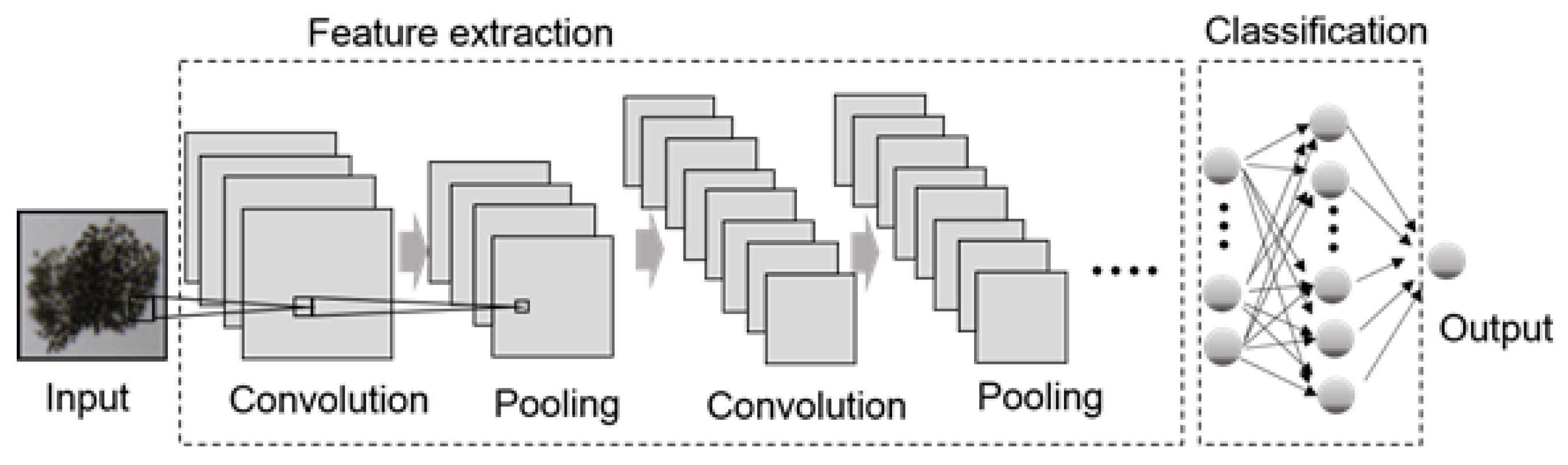More recently, deep learning has been considered as one of the most promising machine learning techniques for image identification and analysis [32,33,34]. Particularly, the convolutional neural network (CNN) is one of the deep neural networks that has been widely applied in image identification and analysis due to its ability to extract and represent high-level abstractions in data sets [33,35,36,37].

For algae image classification, only a few studies were reported in monitoring of algal blooms using CNNs [25,33,38]. For example, Medina et al. [33] applied CNN for algal detection in underwater pipelines which accumulate sand and algae on their surface, hiding damages. They used two classes of algae and non-algae (e.g., sand) and classified the non-algae group with more than 99% accuracy. More recently, Lakshmi and Sivakumar [38] used a CNN model for the classification of Chlorella with 91.82% accuracy. However, the study used CNN architectures that were arbitrarily chosen by researcher’s experience, and did not explore possible CNN architectures which may better fit algal image data.

In this paper, a neural architecture search (NAS), an automatic approach for the design of artificial neural networks (ANN), is used to automatically examine possible CNN architectures and yield a more accurate CNN architecture for algal classification. Ordinary machine learning of ANN is a technique to find weight parameters that fit data, whereas NAS is a technique to find best structural elements (e.g., convolution layer and pooling layer) of ANN. A diverse set of solutions have been developed for NAS [39,40,41]. A recent review paper introduces various techniques for NAS [42]. Such techniques include grid search, random search, evolutionary algorithms, reinforcement learning, and Bayesian optimization. Grid search explores the best parameters among parameter spaces that were manually selected at regular intervals or grids, whereas random search uses random selection for the parameter spaces. Evolutionary algorithms [43] are widely used for any optimization problems to find a best solution. For ANN, comprehensive research [44,45,46,47] of NAS using the evolutionary algorithms have been conducted. Another adaptable method, reinforcement learning [48], has recently taken over from the evolutionary algorithms. Zoph and Le [39] used a controller that constructs candidate architectures of ANN and is updated according to the performance score (e.g., accuracy (see Equation (3) in Section 3.3)) of the previously selected candidate architectures. The controller is another machine learning model in the framework of the reinforcement learning approaches. Zoph and Le [39] used recurrent neural networks [49] as the controller model to estimate the candidate architectures. Baker et al. [50] applied reinforcement learning to CNN models for image classification. One of the most popular approaches for parameter optimization under unknown functions is Bayesian optimization. Recently, Jin et al. [41] introduced NAS for CNN models using Bayesian optimization. In this paper, we use the Bayesian optimization based NAS from Jin et al. [41] and introduce it in Section 2.3.

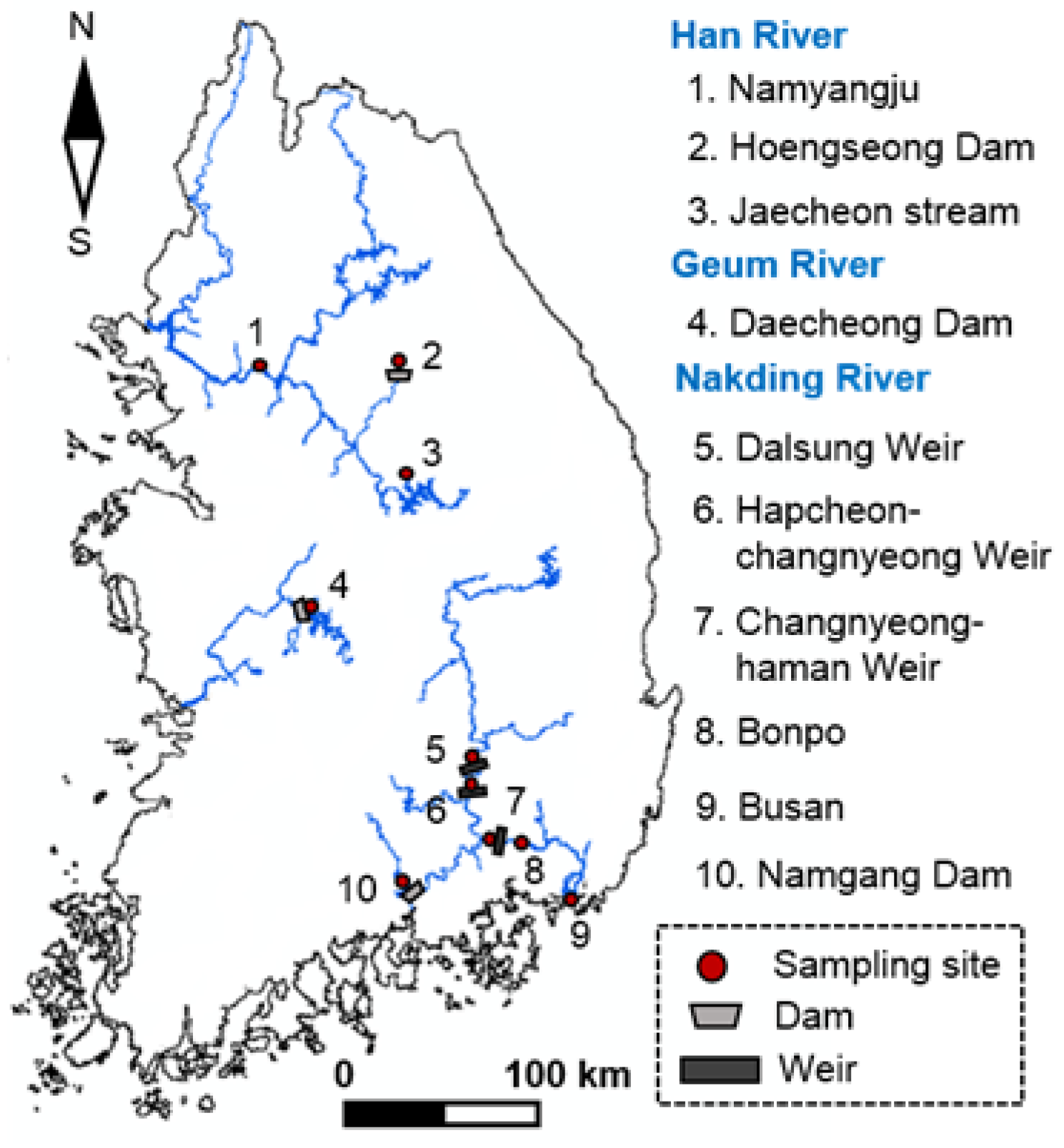
Along with this NAS approach, we introduce a framework which contains three steps (acquisition, preprocessing, and analysis) in order to support the algae image classification based on NAS. In addition, we conduct an experiment in the real-world environment to evaluate the proposed method in this paper. 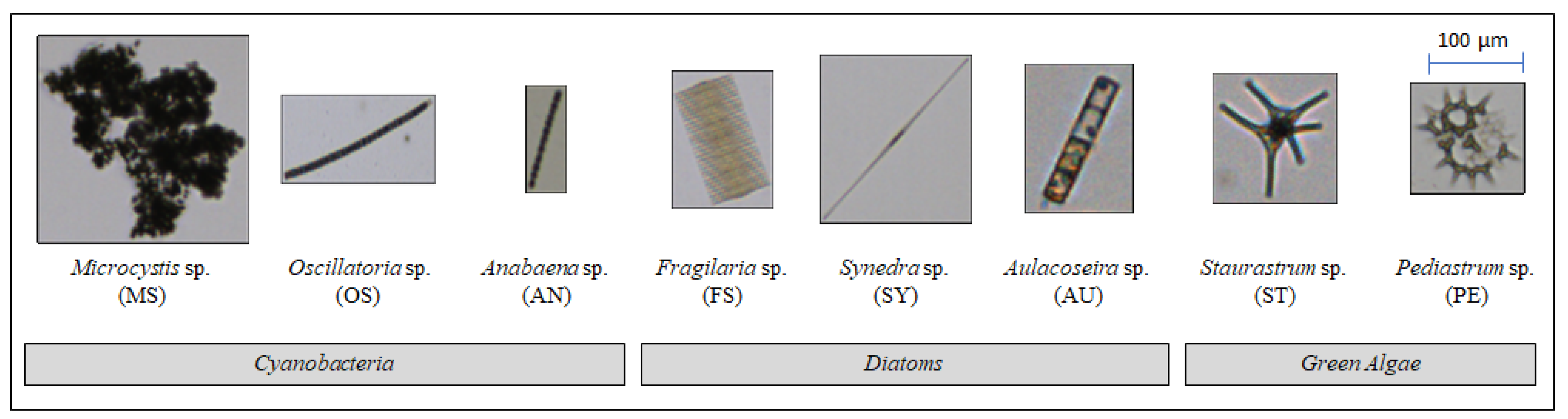First, several tens of thousands of algal images are collected using FlowCAM from various natural water bodies that store run-off during the summer flooding season and provide water supply for domestic, agricultural, and industrial purposes [51]. Then, a CNN model is constructed by NAS and is used to identify eight major algal genera including Microcystis sp., and Oscillatoria sp. found in harmful algal blooms (HABs) events in the major rivers in South Korea. The applicability of the model is verified from two model simulation (experiment) scenarios; (1) using original images only, (2) using augmented images by rotation or mirroring for training and validation. For testing the developed model, original images are used.

In this paper, our contributions are threefold: (i) introducing the neural architecture search approach for algal classification, (ii) suggesting the algal image analysis framework using of machine learning, and (iii) presenting the experimental results from the real-world environments.

2. Background

2.1. CNN Model

A CNN model is composed of input, hidden, and output layers, where the hidden layers are composited with convolution, pooling, and fully-connected layers [33,37,52,53]. Theoretical backgrounds and detailed information regarding CNN can be found elsewhere [36,37,38]. In general, the deep learning for CNN consists of two processes: feature extraction and classification (Figure 1).

In the feature extraction process, the image data is represented as a matrix consisting of M × N, and the image characteristics (or features) are extracted in the convolution and pooling layers (Figure 2). CNN is characterized by the convolution layer, which performs as a filter sliding over the image data and produces filtered data. The convolution layer contains various types of filters (e.g., a vertical edge filter and a horizontal edge filter), which filter out features from the image data. Then, the features are taken as the outputs of the convolution layer. For example, in Figure 2a, the input image data in the matrix form of $7\times 7$ is filtered out using a $3\times 3$ matrix filter. The filter slides over the input data as shown in Figure 2a and an output value in the output matrix is mapped by the Hadamard product (or the entrywise product) [54], followed by adding up the results to obtain the output value. Equation (1) shows an illustrative convolution mapping.

$$O[u,v]=\sum _{m=0}^{M-1}\sum _{n=0}^{N-1}I[u+m,v+n]F[m,n],$$

(1)

where, (1) O, I, and F are the matrices output, input, and filter, respectively, (2) u and v denote the row and column index of O, (3) m and n denote the row and column index of F, and (4) M and N denote the number of rows and columns of F, respectively. After the convolution process, the filtered data can be computed by an activation function to apply the non-linearity, so that the model can reflect non-linear aspects of the data. The outputs from the convolution layer can be inputs to a pooling layer. In the pooling layer, the size of an input is reduced by a pooling rule (e.g., max and average), so that the time of machine learning can be reduced and significant features can be detected among noise (i.e., to develop more robust model). The pooling rule is a simple function that maps a portion of the input data to a value of the output data. For example, a max pooling rule maps from a set of input data {[3, 2], [2, 1, 7]} to a set of output data {[3], [7]}. Figure 2b shows an illustrative example of the max pooling rule in CNN. In Step 1, the max value of seven is selected and mapped to the output matrix. A pair of convolution and pooling processes is repeated several times in the CNN model. Illustrative examples of image outputs in the feature extraction process using microscopic algal images are shown in Figure 3. An overfitting problem often occurs when a trained CNN model fits training data but not test data. A dropout process is then applied to avoid the overfitting problem, in which nodes or units in the network are randomly dropped and trained, so that the trained model can be more generalized [55].

In the classification process, the fully-connected layer is a multi-layer neural network [56] in which all input nodes are connected to all hidden nodes, and the hidden nodes are connected to all output nodes. The output nodes in the fully-connected layers are used to represent classification results (e.g., 85% probability of Microcystis sp. and 15% probability of Fragilaria sp.)

2.2. CNN Architecture for Algal Image Classification

In this subsection, an illustrative example of a CNN architecture for algal image classification is introduced. Note that the example CNN architecture will be used in Section 3 as the name of Manual Model 1. The CNN architecture is composed of four pairs of convolution-pooling layers. The first convolution layer filters the input image with a $150\times 150$ pixel size using 32 filters, and the number of filters in the second, third, and fourth convolution layers are 64, 128, and 128, respectively. The filter sizes are the same for the four convolution layers, as $3\times 3$, and a rectified linear unit activation function, ReLU (Equation (2)), is applied, which overcomes the vanishing gradient problem in conventional artificial neural network and allows faster machine learning [57].

$$f\left(x\right)=\left\{\begin{array}{cc}0\hfill & x<0\hfill \\ x\hfill & x\ge 0\hfill \end{array}\right.$$

(2)

The overall schematic diagram of the CNN architecture is illustrated in Figure 4. The strides (specifying the strides of the convolution along the vertical and horizontal direction at each calculation step) in the convolution layer are defined as $1\times 1$; thus, the model computes the input data by sliding one step aside at a time horizontally and vertically, as indicated in the diagram in Figure 2a. In each pooling layer, the spatial dimension of input image was reduced by a $2\times 2$ filter. After the feature extraction process, the dropout with the probability of 50% is applied to avoid overfitting. The number of nodes (input pixel size) for the classification layer is 6272 ($7\times 7\times 128$) and the final output size is five, as the model is developed for eight different algal genera. The classification is processed by a softmax function, a normalized exponential function which reports each output in the range between 0 and 1, and all the output is added up to one [58].

2.3. Bayesian Optimization Based Neural Architecture Search

Bayesian optimization based Neural Architecture Search (BO-NAS) is a Neural Architecture Search that automatically searches the best architecture of artificial neural networks (ANN) using Bayesian optimization. Bayesian optimization can be used to estimate a black box function, F, in which its expressions and derivatives are unknown. To do that, Bayesian optimization uses two processes: (1) Exploitation and (2) Exploration. Exploitation is a process for modeling an objective function (i.e., the probable black box function) and Exploration is a process for deciding the next investigating point.

In the assumption of the multivariate Gaussian distribution for the black box function, Gaussian process (GP) can be applied in the Exploitation process. Equation (3) shows the Gaussian process [59].

$$P\left(F\left(x\right)\right|D,x)=N(\mu \left(x\right),{\sigma }^2\left(x\right)),$$

(3)

where D denotes observed data $\{x_{1:n},F\left(x_{1:n}\right)\}$, x denotes an independent value for $F(.)$, $\mu (.)$ denotes a mean function of x, and ${\sigma }^2(.)$ denotes a variance function of x. These $\mu (.)$ and ${\sigma }^2(.)$ are shown in Equations (4) and (5), respectively.

$$\mu \left(x\right)={\mathbf{k}}^T{\mathbf{K}}^{-1}F\left(x_{1:n}\right)$$

(4)

and

$${\sigma }^2\left(x\right)=\mathbf{k}(x,x)-{\mathbf{k}}^T{\mathbf{K}}^{-1}\mathbf{k},$$

(5)

where $\mathbf{k}=[k(x,x_1),k(x,x_2),\dots ,k(x,x_n)]$ denotes a set of kernel functions $k(.,.)$ and $\mathbf{K}$ denotes a kernel matrix as shown in Equation (6).

$$\mathbf{K}=\left[\begin{array}{ccc}k(x_1,x_1)& \dots & k(x_1,x_n)\\ \dots & \dots & \dots \\ k(x_n,x_1)& \dots & k(x_n,x_n)\end{array}\right]$$

(6)

In GP, the kernel function performs the important role of representing the black box function [59]. For the GP model, BO-NAS from [41] introduces a specialized kernel function in Equation (7).

$$k(N_a,N_b)=e^{-{\rho }^2\left(d(N_a,N_b)\right)},$$

(7)

where function $d(.,.)$ denotes the distance of two neural networks $N_a$ and $N_b$, and $\rho$ denotes a mapping function between the distance in the original metric space and the distance in the new space [41].

The process of BO-NAS consists of three iterative steps (Update, Generate, and Observe) as shown in Figure 5. In the beginning, default ANN architectures are given to the process. The ANN architectures are trained and validated using training and validation data, respectively. In the step Update, the architectures and the accuracy scores from the validation are used to construct a Gaussian process model (Equation (3)), the generalization of the Gaussian probability distribution [59]. In the step Generate, using the Gaussian process model, potential architectures with its estimated score are generated and an ANN architecture with the highest estimated-score is chosen. Then, the best ANN architecture is trained and validated in the step Observe. These three steps continue until a predefined running time (e.g., 2 h). After this, the best ANN architecture in the history of the ANN architectures is selected as a final output.

3. Framework of Machine Learning Analysis for Algae Images

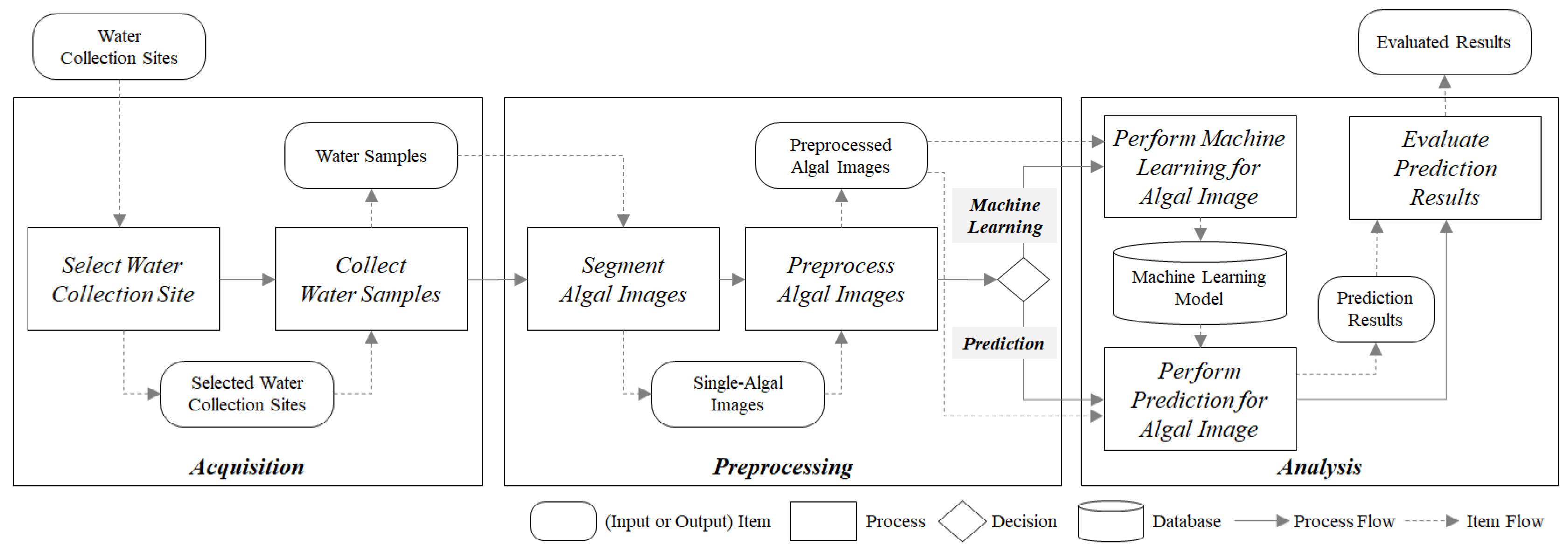
Developing classification models (e.g., CNN models) can be greatly facilitated by the use of a generic framework, which provides a guideline for the development of the classification models and especially focuses on analysis of algal images. In this section, we introduce a framework of machine learning analysis for algal images (Figure 6). The framework consists of three main processes: (1) acquisition, (2) preprocessing, and (3) analysis. The inputs of the framework are the water collecting sites (e.g., the stream or reservoir), and the outputs of the framework are the evaluated results from the algal image analysis.

3.1. Acquisition

The acquisition step defines water collection sites and performs the collection of water samples. In this step, one should define purposes of the algal image analysis (e.g., algal image classification, harmful algae detection, and algal quantity analysis). Then, one should select major places where the target algae inhabit. This step outputs water samples by means of water collection techniques (e.g., [60,61]).

3.2. Preprocessing

The preprocessing step aims at generating proper image data for analysis (i.e., machine learning and prediction) in the next step. The water samples from the acquisition step are captured as image data. Then, the image data are segmented according to the purpose of analysis. These sub-steps can be automated by using FlowCAM, which includes image capturing and segmentation capability. The preprocessing step contains image transformation (e.g., augmentation). Image data augmentation is the process of generating more data from the original data. In deep learning, a large dataset is crucial for model generalization, fitting well on unseen data. For image data augmentation, it is possible to apply several data transformation techniques (e.g., mirroring, rotating, scaling, and adding noise) to the original data.

3.3. Analysis

The analysis step consists of three sub-steps: (1) perform machine learning, (2) perform prediction, and (3) evaluate prediction results. In the sub-step “perform machine learning”, machine learning models (e.g., random forests [62], Gaussian naive Bayes [63], and support vector machine [64]) are developed. Note that in this paper, we focus on the CNN model, a state-of-the-art deep learning model for image classification. To measure the performance of such analysis models, performance metrics are required. We introduce some performance metrics for classification.

As a classification performance metrics, the accuracy Acc of Equation (3), the sum of correct classification divided by the total number of classifications, can be used.

$$Acc=\frac{Thenumberofcorrectclassification}{Thetotalnumberofclassification}=\frac{{\sum }_{i=1}^N{x}_{ij}}{{\sum }_{i=1}^N{\sum }_{j=1}^N{x}_{ij}},$$

(8)

where N denotes the number of class and $x_{ij}$ denotes the total number of the case in which values of i-th prediction and j-th observation are identical. Except the accuracy score Acc, we can use precision (Equation (4)), recall (Equation (5)), and F1-score (Equation (6)). These metrics can be easily calculated by using the following four indicators (TP, FP, FN and TN).

• True positive (TP): the amount of the observed positive values which were correctly predicted,
• False positive (FP): the amount of the observed positive values which were wrongly predicted,
• False negative (FN): the amount of the observed negative values which were wrongly predicted,
• True negative (TN): the amount of the observed negative values which were correctly predicted.

These four indicators can be used to define the equations of Precision and Recall as shown.

$$\mathrm{Precision}=\frac{\mathrm{TP}}{\mathrm{TP}+\mathrm{FP}}$$

(9)

$$\mathrm{Recall}=\frac{\mathrm{TP}}{\mathrm{TP}+\mathrm{FN}}.$$

(10)

Precision is commonly used to measure the influence of false positives, while Recall is used to measure the influence of false negatives. F1-score is defined as the weighted average of Precision and Recall.

$$\mathrm{F}1-\mathrm{score}=\frac{2\times (\mathrm{Precision}\times \mathrm{Recall})}{\mathrm{Precision}+\mathrm{Recall}}.$$

(11)

Precision, Recall, and F1-score have a score of one when the prediction is perfect. For the total prediction failure, they yield a score of zero.

After the sub-step Perform Machine Learning, the learned machine learning models are stored in a database. The database is activated to output the learned machine learning models, when inputting the request of prediction and input data in the sub-step Perform Prediction. Then, prediction results (e.g., classification results) are output from the sub-step Perform Prediction and evaluated using the purposes of the algal image analysis defined in the step Acquisition.

4. Experiment in the Real-World Environments

In 2015, Korea Water Resources Corporation (K-water) conducted a project regarding algal species identification to support direct and continuous monitoring in water management districts and utilities for processing drinking water. In this project, a novel approach combining the CNN and NAS technologies were used to identify harmful algae where input algal images data were collected using a FlowCAM. Thus, the novel technique can support a rapid and unbiased identification of algal status in bloom events. Our experiment follows the framework of machine learning analysis for algae images introduced in Section 3.

4.1. Acquisition

4.1.1. Select Water Sample Collection Sites

Ten sites in natural rivers or reservoirs were selected for water sample collection (Figure 7). These sites were located in the three major rivers (Han River, Geum River, and Nakding River) of South Korea, where algal bloom events occurr frequently.

4.1.2. Water Sample Collection

For four years between 2015 and 2018, water samples were arbitrarily collected in the ten sites we chose (Figure 7 and

Table 1. Sampling sites in South Korea for the convolutional neural network (CNN) model development.

Watershed	Site	Collected Algal Genus
Han River	Namyangju, Gyeonggi-do (Site 1)	FS, OS, PE, AU, ST
	Hoengseong Dam (Site 2)	SY
	Jaecheon Stream (Site 3)	OS, AN
Geum River	Daecheong Dam (Site 4)	MS
Nakdong River	Dalsung Weir (Site 5)	MS
	Hapcheon-changnyeong Weir (Site 6)	MS
	Changnyeong-haman Weir (Site 7)	MS
	Bonpo, Gyeongsangnam-do (Site 8)	SY
	Busan (Site 9)	MS
	Namgang Dam (Site 10)	FS

) when algal bloom occurred.

4.2. Preprocessing

4.2.1. Segment Algal Images

To segment algal images, a FlowCAM (Flow Cytometer and Microscope, Fluid Imaging Technologies, Yarmouth, ME, USA), ×40 microscope with a commercial particle image analyzer, was used. A total of 1922 photographic morphological images of eight different algal genera were detected from the water samples using the FlowCAM (

Table 2. The number of images for each algal species captured by the FlowCAM.

MS	OS	AN	FS	SY	AU	ST	PE
360	270	120	360	360	50	42	360

). The eight algal genera included three cyanobacteria (Microcystis sp. (MS), Oscillatoria sp. (OS), and Anabaena sp. (AN)), three diatoms (Fragilaria sp. (FS), Synedra sp. (SY), and Aulacoseira sp. (AU)), and two green algae (Staurastrum sp. (ST) and Pediastrum sp. (PE)) as shown in Figure 8. Microcystis sp., Oscillatoria sp. and Anabaena sp. as common cyanobacterial species were selected as they are typically observed in freshwater HABs. These three species release toxins that have adverse effects on drinking water quality. Synedra sp. was selected as it causes clogging problems in the filtering system of drinking water treatment plants.

4.2.2. Preprocess Algal Images

In this step, we transformed the algal images for the image analysis. Some algal images from the FlowCAM contained border lines that can affect the analysis. So, the border lines were trimmed. The various formats of the images, then, were converted to one image format (PNG (Portable Network Graphics)).

For the image analysis, two groups of data were used: (1) the original image data and (2) the augmented image data, so that we could compare the effects of data augmentation and would be able to improve the model accuracy. Also, for CNN machine learning, the images data were classified into three categories (training, validation, and test). The details of the data settings are as follows.

• Original data 1158 (60%), 382 (20%), and 382 (20%) original images were used for the training, the validation, and the test, respectively.
• Augmented data 5790 and 1910 images augmented from the original images by mirroring, rotating, and top-down flipping were used for the training and the validation, respectively. The 382 original images were used for the test.

4.2.3. Perform Machine Learning for Algal Image

Three machine learning experiments were conducted for each data group (original and augmented). For each experiment, a different CNN architecture was used. The two architectures were manually developed as in the previous research [25], while the last architecture was generated from NAS. The details of the architecture settings are as follows.

• Experiment 1 (manual model 1): one CNN model was manually developed by trial and error. The model was developed from scratch and was used in Experiment 1.
• Experiment 2 (manual model 2): one CNN model was also manually developed by trial and error. The model was developed based on the popular model (LeNet [65]) and was used in Experiment 2.
• Experiment 3 (NAS model): two CNN models, simply called NAS models, were developed by using neural architecture search in Section 2.3. NAS model 1 used the original data, while NAS model 2 used the augmented data.

Each experiment required parameter settings to perform machine learning.

Table 3. Machine learning parameter settings for CNN.

Experiment	Learning Rate	Max Epochs	Running Time
Manual Model 1	0.001	12	-
Manual Model 2	0.001	12	-
NAS Model 1	0.001	12	1 h
NAS Model 2	0.001	12	1 h

shows the machine learning parameter settings that we used for the experiments.

The experiments were run on a 3.40 GHz Intel Core i7-3770 processor. For NAS, the total searching time was 1 hour. The validation data proportion, denoting the proportion of the validation data from the training data, was 0.05. The maximum number of epochs to train the CNN architectures was 12. The training would stop when this number was reached. The learning rate of the training was 0.001.

Table 4. The architectures used for the experiments.

Layers	Manual Model 1	Manual Model 2	NAS Model 1	NAS Model 2
Convolution	4	4	6	3
Pooling	4	2	5	3
Fully Connected	2	2	4	2

shows the layer information of the architectures used for the experiments. Manual 1 and 2 denote the architectures in Experiment 1 and 2, respectively. NAS 1 denotes the architecture found by neural architecture search using the original data, while NAS 2 means the architecture from the augmented data.

4.2.4. Perform Prediction for Algal Image

In this step, the trained CNN model in Section 4.2.3 was used to predict the class of an algal image. For this, the test data prepared in Section 4.2.2 were used.

4.2.5. Evaluate Prediction Results

In this paper, the three-performance metrics precision (Equation (4)), recall (Equation (5)), and F1-score (Equation (6)) were used to show the performance of the algal image classification.

Table 5. Manual model 1 (the original data).

Type	F1-score	Precision	Recall	#
AN	0	0	0	24
AU	0	0	0	10
FS	0.9	0.83	0.99	72
MS	1	1	1	72
OS	0.7	0.56	0.92	52
PE	0.92	1	0.85	72
ST	0.46	0.6	0.38	8
SY	1	1	1	72
Avg.	0.6225	0.6238	0.6425	47.75

,

Table 6. Manual model 2 (the original data).

Type	F1-score	Precision	Recall	#
AN	0.57	0.47	0.71	24
AU	0.18	1	0.1	10
FS	0.96	1	0.92	72
MS	1	1	1	72
OS	0.81	0.8	0.83	52
PE	0.99	0.99	1	72
ST	0.75	0.75	0.75	8
SY	1	1	1	72
Avg.	0.7825	0.8763	0.7888	47.75

,

Table 7. Neural architecture search (NAS) model 1 (the original data).

Type	F1-score	Precision	Recall	#
AN	0.86	1	0.75	24
AU	0.95	0.91	1	10
FS	0.98	0.96	1	72
MS	1	1	1	72
OS	0.95	0.9	1	52
PE	0.98	1	0.96	72
ST	0.93	1	0.88	8
SY	1	1	1	72
Avg.	0.9563	0.9713	0.9488	47.75

,

Table 8. Manual model 1 (the augmented data).

Type	F1-score	Precision	Recall	#
AN	0.57	0.56	0.58	24
AU	0.13	0.2	0.1	10
FS	0.82	0.91	0.74	72
MS	1	1	1	72
OS	0.82	0.69	1	52
PE	0.96	1	0.92	72
ST	0.67	0.71	0.62	8
SY	0.99	0.97	1	72
Avg.	0.745	0.755	0.745	47.75

,

Table 9. Manual model 2 (the augmented data).

Type	F1-score	Precision	Recall	#
AN	0.26	0.57	0.17	24
AU	0.8	0.8	0.8	10
FS	0.97	0.97	0.97	72
MS	1	1	1	72
OS	0.85	0.73	1	52
PE	0.99	1	0.97	72
ST	0.88	0.88	0.88	8
SY	1	1	1	72
Avg.	0.8438	0.8688	0.8488	47.75

and

Table 10. NAS model 2 (the augmented data).

Type	F1-score	Precision	Recall	#
AN	0.94	0.96	0.92	24
AU	0.82	1	0.7	10
FS	0.94	0.98	0.9	72
MS	1	1	1	72
OS	0.93	0.88	0.98	52
PE	0.98	0.97	0.99	72
ST	0.84	0.73	1	8
SY	1	1	1	72
Avg.	0.9313	0.94	0.9363	47.75

show the experiment results of the classification using the four CNN architectures (manual model 1, manual model 2, NAS model 1, and NAS model 2). For example, Table 5 shows the classification results using the manual model 1 and the original data. In this case, the average precision and the average recalls were 0.6238 and 0.6425, respectively. As another example, Table 10 shows the classification results using the NAS model 2 and the augmented data (the average precision: 0.94 and the average recall: 0.9363).

All F1-Score results are summarized in

Table 11. F1-Scores.

Data	Manual Model 1	Manual Model 2	NAS Models 1 and 2
Original	0.6225	0.7825	0.9563
Augmented	0.745	0.8438	0.9313

. Generally, we noticed that the results from the augmented data outperformed the result of using only original data in the case of manual model 1 and manual model 2. This indicates that the image augmentation partially helps the performance of image classification. However, the image augmentation did not always lead to higher performance results, since in some cases unobservable images could be generated by augmentation, thus hindering proper classification. Through several repeated experiments, we confirmed that the NAS model 1 using only the original data performed better than the NAS model 2 using the augmented data.

The F1-Scores from the experiment using neural architecture search were fairly higher than the results by using only the manual modeling approach. Consequently, neural architecture search always led to higher performance.

Figure 9 shows six confusion matrices for each CNN model evaluation (corresponding to Table 5, Table 6, Table 7, Table 8, Table 9 and Table 10), where the the X axis denotes the predicted class using the trained CNN model, the Y axis denotes the observed class in the test data, and each numbered cell denotes the total number of the case in which the predicted class and the observed class are identical. When looking at the visualization of these confusion matrices, we can clearly notice which algal species was misclassified. The manually developed CNN models especially misclassified the three algal species (Anabaena sp., Aulacoseira sp., and Oscillatoria sp.) with similar linear shapes.

5. Discussion for the Algal Image Classification

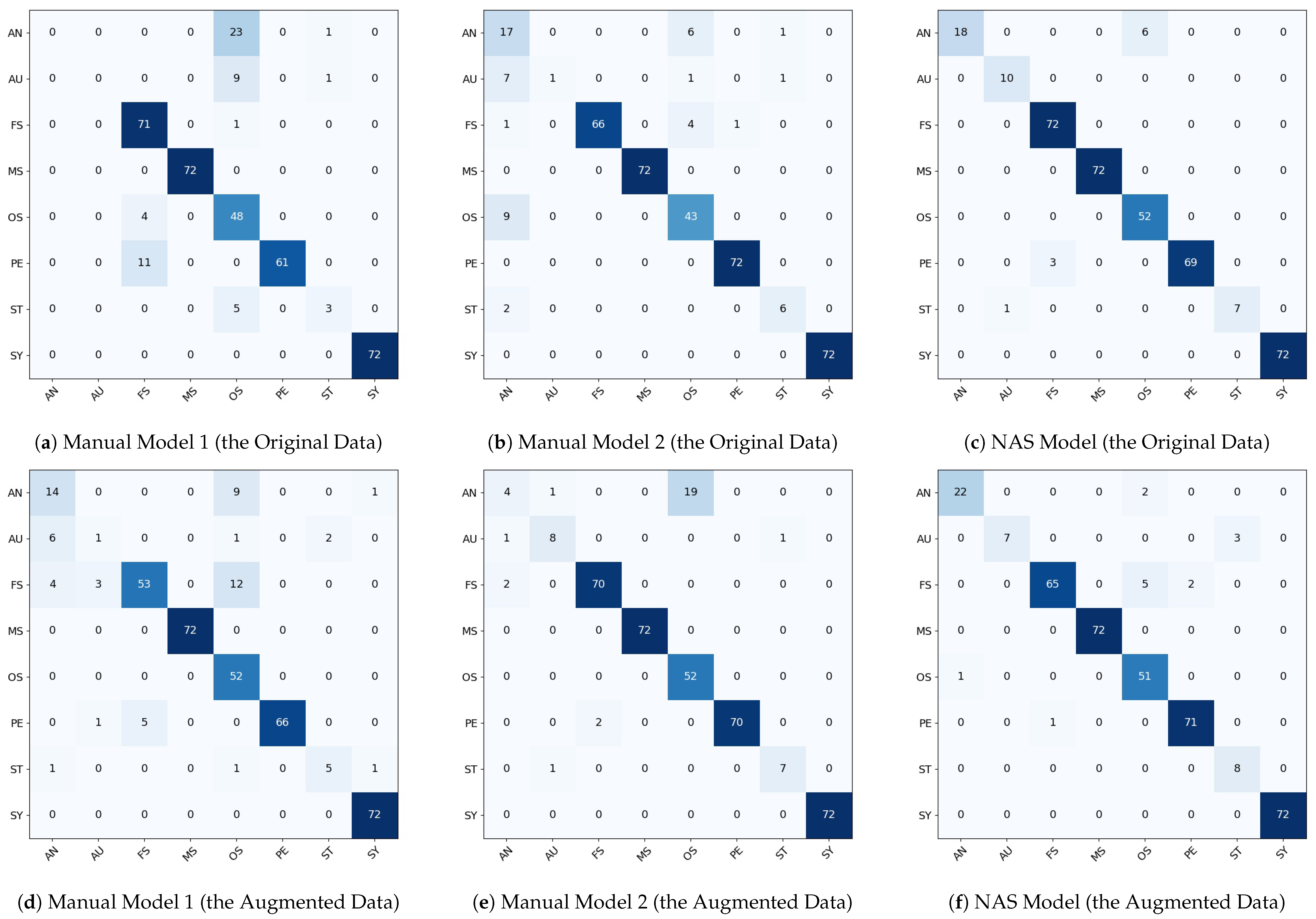
In this study, four CNN models were developed for the classification of representative algal genera of HABs from algal images obtained using FlowCAM. The NAS models developed in this paper classified the eight algal genera effectively in comparison to the manually developed models.

The results verified the applicability of the NAS technology for the analysis of algal cells at the genus level. The average F1-Score for the NAS model 1 was 0.9563 to classify the eight algal classes. This result indicated that the NAS technology can outperform the conventional CNN modeling approach. Also, the developed CNN model may be further optimized depending on the algal image library, which is used for the classification, as we can see the performance improvement of using the augmented data.

In this paper, we focused on algal image classification based on the NAS technology and its framework to lead and guide one to efficient research and applications. However, there are several future research topics. First, the CNN model developed in this study classified eight algal genera commonly found in HABs events, with no interference effect from the additional images which were not included in our model library. CNN models can misclassify images which are not included in the model library, thus reducing the reliability of the CNN model. For this, we can consider an image library platform for algal species. Obviously, the CNN model applicability can be improved by increasing the number of microscopic algal images with different algal species. Secondly, in the current development of the CNN model, there was no consideration of microalgal colonies. However, for example, a Microcystis sp. colony typically consists of hundreds to thousands of individual algal cells. Counting individual algal cells in a colony is important to determine the physiological status of the algal bloom in freshwater systems, and is included in guidelines for general algal management [66,67]. To the best of our knowledge, no studies have been reported for developing automated algal cell counts. It seems that recent deep learning techniques may provide a possible approach. For example, one of the recent deep-learning techniques, U-net, is used for the segmentation of images and has been applied in the medical field [68,69,70]. This may provide a possible solution for individual cell counting in the Microcystis sp. colonies. As this method is still in the early stages of research, further studies are suggested to extend the possible application of deep learning techniques as a novel method for algal bloom monitoring.

6. Conclusions

In this paper, our research showed that the well-defined CNN model generated from the neural architecture search technology can be an alternative technique to replace conventional manual CNN modeling methods for algal classification for HABs monitoring in watersheds. In practice, the presented approach can rapidly and accurately classify algal species for the effective management of drinking water treatment processes. The presented models classified the eight algal genera with up to the F1-score of 0.95, thereby suggesting the possible applicability of CNN and NAS for algal classification in practice. It was expected that this new procedure using the CNN model would provide a rapid and reliable algal classification method, and also enable real-time monitoring and early warning of HABs in their watersheds. In addition, we introduced the novel framework of machine learning analysis for algal images to guide researchers and data analysts. The framework was applied to the real-world situations in South Korea. Further extension on developing algal image libraries with more algal species in various field sites would improve the applicability of the model in real-world simulations and is left for future research.

References

1. Dauta, A.; Devaux, J.; Piquemal, F.; Boumnich, L. Growth rate of four freshwater algae in relation to light and temperature. Hydrobiologia 1990, 207, 221–226. [Google Scholar] [CrossRef]
2. Paerl, H.W.; Huisman, J. Blooms like it hot. Science 2008, 320, 57–58. [Google Scholar] [CrossRef] [PubMed]
3. Paerl, H.W.; Otten, T.G. Harmful cyanobacterial blooms: causes, consequences, and controls. Microb. Ecol. 2013, 65, 995–1010. [Google Scholar] [CrossRef] [PubMed]
4. Robarts, R.D.; Zohary, T. Temperature effects on photosynthetic capacity, respiration, and growth rates of bloom-forming cyanobacteria. N. Z. J. Mar. Freshw. Res. 1987, 21, 391–399. [Google Scholar] [CrossRef]
5. Cao, J.; Chu, Z.; Du, Y.; Hou, Z.; Wang, S. Phytoplankton dynamics and their relationship with environmental variables of Lake Poyang. Hydrol. Res. 2016, 47, 249–260. [Google Scholar] [CrossRef] [Green Version]
6. Dove, A.; Chapra, S.C. Long-term trends of nutrients and trophic response variables for the Great Lakes. Limnol. Oceanogr. 2015, 60, 696–721. [Google Scholar] [CrossRef]
7. Zhang, C.; Lai, S.; Gao, X.; Xu, L. Potential impacts of climate change on water quality in a shallow reservoir in China. Environ. Sci. Pollut. Res. 2015, 22, 14971–14982. [Google Scholar] [CrossRef]
8. Dittmann, E.; Wiegand, C. Cyanobacterial toxins–occurrence, biosynthesis and impact on human affairs. Mol. Nutr. Food Res. 2006, 50, 7–17. [Google Scholar] [CrossRef]
9. Shen, Q.; Zhu, J.; Cheng, L.; Zhang, J.; Zhang, Z.; Xu, X. Enhanced algae removal by drinking water treatment of chlorination coupled with coagulation. Desalination 2011, 271, 236–240. [Google Scholar] [CrossRef]
10. World Health Organization. Guidelines for Drinking-Water Quality; World Health Organization: Geneva, Switzerland, 2004; Volume 1. [Google Scholar]
11. Jančula, D.; Maršálek, B. Critical review of actually available chemical compounds for prevention and management of cyanobacterial blooms. Chemosphere 2011, 85, 1415–1422. [Google Scholar] [CrossRef]
12. Li, F.; Liang, Z.; Zheng, X.; Zhao, W.; Wu, M.; Wang, Z. Toxicity of nano-TiO2 on algae and the site of reactive oxygen species production. Aquat. Toxicol. 2015, 158, 1–13. [Google Scholar] [CrossRef] [PubMed]
13. Park, J.; Church, J.; Son, Y.; Kim, K.T.; Lee, W.H. Recent advances in ultrasonic treatment: challenges and field applications for controlling harmful algal blooms (HABs). Ultrason. Sonochem. 2017, 38, 326–334. [Google Scholar] [CrossRef] [PubMed]
14. Purcell, D.; Parsons, S.A.; Jefferson, B.; Holden, S.; Campbell, A.; Wallen, A.; Chipps, M.; Holden, B.; Ellingham, A. Experiences of algal bloom control using green solutions barley straw and ultrasound, an industry perspective. Water Environ.J. 2013, 27, 148–156. [Google Scholar] [CrossRef]
15. Boylan, J.D.; Morris, J.E. Limited effects of barley straw on algae and zooplankton in a midwestern pond. Lake Reserv. Manag. 2003, 19, 265–271. [Google Scholar] [CrossRef]
16. Zamyadi, A.; Choo, F.; Newcombe, G.; Stuetz, R.; Henderson, R.K. A review of monitoring technologies for real-time management of cyanobacteria: Recent advances and future direction. TrAC Trends Anal. Chem. 2016, 85, 83–96. [Google Scholar] [CrossRef]
17. Goldberg, S.J.; Kirby, J.T.; Licht, S.C. Applications of Aerial Multi-Spectral Imagery for Algal Bloom Monitoring in Rhode Island; SURFO Technical Report No. 16-01; Graduate School of Oceanography: Narragansett, RI, USA, 2016; p. 28. [Google Scholar]
18. Kudela, R.M.; Palacios, S.L.; Austerberry, D.C.; Accorsi, E.K.; Guild, L.S.; Torres-Perez, J. Application of hyperspectral remote sensing to cyanobacterial blooms in inland waters. Remote Sens. Environ. 2015, 167, 196–205. [Google Scholar] [CrossRef] [Green Version]
19. Lekki, J.; Anderson, R.; Avouris, D.; Becker, R.; Churnside, J.; Cline, M.; Demers, J.; Leshkevich, G.; Liou, L.; Luvall, J.; et al. Airborne Hyperspectral Sensing of Monitoring Harmful Algal Blooms in the Great Lakes Region: System Calibration and Validation; NASA: Washington, DC, USA, 2017.
20. Le Bourg, B.; Cornet-Barthaux, V.; Pagano, M.; Blanchot, J. FlowCAM as a tool for studying small (80–1000 μm) metazooplankton communities. J. Plankton Res. 2015, 37, 666–670. [Google Scholar] [CrossRef]
21. Álvarez, E.; Moyano, M.; López-Urrutia, Á.; Nogueira, E.; Scharek, R. Routine determination of plankton community composition and size structure: A comparison between FlowCAM and light microscopy. J. Plankton Res. 2013, 36, 170–184. [Google Scholar] [CrossRef]
22. Poulton, N.J. FlowCam: Quantification and classification of phytoplankton by imaging flow cytometry. In Imaging Flow Cytometry; Springer: Berlin, Gremany, 2016; pp. 237–247. [Google Scholar]
23. Romero-Martínez, L.; van Slooten, C.; Nebot, E.; Acevedo-Merino, A.; Peperzak, L. Assessment of imaging-in-flow system (FlowCAM) for systematic ballast water management. Sci. Total Environ. 2017, 603, 550–561. [Google Scholar] [CrossRef]
24. Dashkova, V.; Malashenkov, D.; Poulton, N.; Vorobjev, I.; Barteneva, N.S. Imaging flow cytometry for phytoplankton analysis. Methods 2017, 112, 188–200. [Google Scholar] [CrossRef]
25. Li, X.; Liao, R.; Zhou, J.; Leung, P.T.; Yan, M.; Ma, H. Classification of morphologically similar algae and cyanobacteria using Mueller matrix imaging and convolutional neural networks. Appl. Opt. 2017, 56, 6520–6530. [Google Scholar] [CrossRef] [PubMed]
26. Bhattacharya, B.; Price, R.; Solomatine, D. Machine learning approach to modeling sediment transport. J. Hydraul. Eng. 2007, 133, 440–450. [Google Scholar] [CrossRef]
27. Dawson, C.; Wilby, R. Hydrological modelling using artificial neural networks. Prog. Phys. Geogr. 2001, 25, 80–108. [Google Scholar] [CrossRef]
28. Huang, J.; Gao, J.; Zhang, Y. Combination of artificial neural network and clustering techniques for predicting phytoplankton biomass of Lake Poyang, China. Limnology 2015, 16, 179–191. [Google Scholar] [CrossRef]
29. Maier, H.R.; Jain, A.; Dandy, G.C.; Sudheer, K.P. Methods used for the development of neural networks for the prediction of water resource variables in river systems: current status and future directions. Environ. Model. Softw. 2010, 25, 891–909. [Google Scholar] [CrossRef]
30. Singh, B.; Sihag, P.; Singh, K. Modelling of impact of water quality on infiltration rate of soil by random forest regression. Model. Earth Syst. Environ. 2017, 3, 999–1004. [Google Scholar] [CrossRef]
31. Support vector machines in water quality management. Anal. Chim. Acta 2011, 703, 152–162. [CrossRef] [PubMed]
32. Chapelais-Baron, M.; Goubet, I.; Péteri, R.; de Fatima Pereira, M.; Mignot, T.; Jabveneau, A.; Rosenfeld, E. Colony analysis and deep learning uncover 5-hydroxyindole as an inhibitor of gliding motility and iridescence in Cellulophaga lytica. Microbiology 2018, 164, 308–321. [Google Scholar] [CrossRef] [PubMed]
33. Medina, E.; Petraglia, M.R.; Gomes, J.G.R.; Petraglia, A. Comparison of CNN and MLP classifiers for algae detection in underwater pipelines. In Proceedings of the 2017 Seventh IEEE International Conference on Image Processing Theory, Tools and Applications (IPTA), Montreal, QC, Canada, 28 Novemner–1 December 2017; pp. 1–6. [Google Scholar]
34. Salman, A.; Jalal, A.; Shafait, F.; Mian, A.; Shortis, M.; Seager, J.; Harvey, E. Fish species classification in unconstrained underwater environments based on deep learning. Limnol. Oceanogr. Methods 2016, 14, 570–585. [Google Scholar] [CrossRef] [Green Version]
35. Cireşan, D.; Meier, U.; Schmidhuber, J. Multi-column deep neural networks for image classification. arXiv 2012. Available online: https://arxiv.org/abs/1202.2745 (accessed on 27 June 2019).
36. Krizhevsky, A.; Sutskever, I.; Hinton, G.E. Imagenet classification with deep convolutional neural networks. In Advances in Neural Information Processing Systems; MIT Press: Cambridge, MA, USA, 2012; pp. 1097–1105. [Google Scholar]
37. Zeiler, M.D.; Fergus, R. Visualizing and Understanding Convolutional Networks. In Computer Vision–ECCV 2014; Fleet, D., Pajdla, T., Schiele, B., Tuytelaars, T., Eds.; Springer International Publishing: Cham, Switzerland, 2014; pp. 818–833. [Google Scholar] [Green Version]
38. Lakshmi, S.; Sivakumar, R. Chlorella Algae Image Analysis Using Artificial Neural Network and Deep Learning. In Biologically Rationalized Computing Techniques For Image Processing Applications; Springer: Berlin, Germany, 2018; pp. 215–248. [Google Scholar]
39. Zoph, B.; Le, Q.V. Neural architecture search with reinforcement learning. arXiv 2016, arXiv:1611.01578. [Google Scholar]
40. Zoph, B.; Vasudevan, V.; Shlens, J.; Le, Q.V. Learning transferable architectures for scalable image recognition. In Proceedings of the IEEE Conference on Computer Vision and Pattern Recognition, Salt Lake City, UT, USA, 18–22 June 2018; pp. 8697–8710. [Google Scholar]
41. Jin, H.; Song, Q.; Hu, X. Efficient neural architecture search with network morphism. arXiv 2018. Available online: https://arxiv.org/abs/1806.10282 (accessed on 27 June 2019).
42. Elsken, T.; Metzen, J.H.; Hutter, F. Neural architecture search: A survey. J. Mach. Learn. Res. 2019, 20, 1–21. [Google Scholar]
43. Holland, J.H. Adaptation in Natural and Artificial Systems: An Introductory Analysis with Applications to Biology, Control, and Artificial Intelligence; MIT Press: Cambridge, MA, USA, 1992. [Google Scholar]
44. Stanley, K.O.; Miikkulainen, R. Evolving neural networks through augmenting topologies. Evol. Comput. 2002, 10, 99–127. [Google Scholar] [CrossRef] [PubMed]
45. Floreano, D.; Dürr, P.; Mattiussi, C. Neuroevolution: from architectures to learning. Evol. Intell. 2008, 1, 47–62. [Google Scholar] [CrossRef]
46. Stanley, K.O.; D’Ambrosio, D.B.; Gauci, J. A hypercube-based encoding for evolving large-scale neural networks. Artif. Life 2009, 15, 185–212. [Google Scholar] [CrossRef] [PubMed]
47. Stanley, K.O.; Clune, J.; Lehman, J.; Miikkulainen, R. Designing neural networks through neuroevolution. Nat. Mach. Intell. 2019, 1, 24–35. [Google Scholar] [CrossRef]
48. Kaelbling, L.P.; Littman, M.L.; Moore, A.W. Reinforcement learning: A survey. J. Artif. Intell. Res. 1996, 4, 237–285. [Google Scholar] [CrossRef]
49. Hopfield, J.J. Neural networks and physical systems with emergent collective computational abilities. Proc. Natl. Acad. Sci. USA 1982, 79, 2554–2558. [Google Scholar] [CrossRef] [PubMed]
50. Baker, B.; Gupta, O.; Naik, N.; Raskar, R. Designing neural network architectures using reinforcement learning. arXiv 2016. Available online: https://arxiv.org/abs/1611.02167 (accessed on 27 June 2019).
51. Park, J.; Wang, D.; Lee, W.H. Evaluation of weir construction on water quality related to algal blooms in the Nakdong River. Environ. Earth Sci. 2018, 77, 408. [Google Scholar] [CrossRef]
52. Kalchbrenner, N.; Grefenstette, E.; Blunsom, P. A convolutional neural network for modelling sentences. In Proceedings of the 52nd Annual Meeting of the Association for Computational Linguistics, Baltimore, MD, USA, 23–25 June 2014; pp. 655–665. [Google Scholar]
53. Oquab, M.; Bottou, L.; Laptev, I.; Sivic, J. Learning and transferring mid-level image representations using convolutional neural networks. In Proceedings of the IEEE Conference on Computer Vision and Pattern Recognition, Columbus, OH, USA, 24–27 June 2014; pp. 1717–1724. [Google Scholar]
54. Horn, R.A. The hadamard product. Proc. Symp. Appl. Math 1990, 40, 87–169. [Google Scholar]
55. Srivastava, N.; Hinton, G.; Krizhevsky, A.; Sutskever, I.; Salakhutdinov, R. Dropout: A Simple Way to Prevent Neural Networks from Overfitting. J. Mach. Learn. Res. 2014, 15, 1929–1958. [Google Scholar]
56. Haykin, S. Neural Networks: A Comprehensive Foundation; Prentice Hall PTR: Upper Saddle River, NJ, USA, 1994. [Google Scholar]
57. Nair, V.; Hinton, G.E. Rectified linear units improve restricted boltzmann machines. In Proceedings of the 27th International Conference on Machine Learning (ICML-10), Haifa, Israel, 21–24 June 2010; pp. 807–814. [Google Scholar]
58. Bishop, C.M. Pattern Recognition and Machine Learning; Springer: Berlin, Germany, 2006. [Google Scholar]
59. Rasmussen, C.E. Gaussian Processes in Machine Learning; Summer School on Machine Learning; Springer: Berlin, Germany, 2003; pp. 63–71. [Google Scholar]
60. Madrid, Y.; Zayas, Z.P. Water sampling: Traditional methods and new approaches in water sampling strategy. TrAC Trends Anal. Chem. 2007, 26, 293–299. [Google Scholar] [CrossRef]
61. S liwka Kaszyńska, M.; Kot-Wasik, A.; Namieśnik, J. Preservation and Storage of Water Samples; Taylor & Francis: London, UK, 2003. [Google Scholar]
62. Breiman, L. Random forests. Mach. Learn. 2001, 45, 5–32. [Google Scholar] [CrossRef]
63. John, G.H.; Langley, P. Estimating continuous distributions in Bayesian classifiers. In Proceedings of the Eleventh Conference on Uncertainty in Artificial Intelligence, Montreal, QU, Canada, 18–20 August 1995; Morgan Kaufmann Publishers Inc.: Burlington, MA, USA, 1995; pp. 338–345. [Google Scholar]
64. Suykens, J.A.; Vandewalle, J. Least squares support vector machine classifiers. Neural Process. Lett. 1999, 9, 293–300. [Google Scholar] [CrossRef]
65. LeCun, Y.; Bottou, L.; Bengio, Y.; Haffner, P. Gradient-based learning applied to document recognition. Proc. IEEE 1998, 86, 2278–2324. [Google Scholar] [CrossRef] [Green Version]
66. Bartram, J.; Chorus, I. Toxic Cyanobacteria in Water: A Guide to Their Public Health Consequences, Monitoring and Management; CRC Press: Boca Raton, FL, USA, 1999. [Google Scholar]
67. National Health and Medical Research Council AG. Guidelines for Managing Risks in Recreational Water; National Health and Medical Research Council AG, Ed.; Australian Government: Canberra, Australia, 2008.
68. Milletari, F.; Navab, N.; Ahmadi, S.A. V-net: Fully convolutional neural networks for volumetric medical image segmentation. In Proceedings of the 2016 IEEE Fourth International Conference on 3D Vision (3DV), Stanford, CA, USA, 25–28 October 2016; pp. 565–571. [Google Scholar]
69. Norman, B.; Pedoia, V.; Majumdar, S. Use of 2D U-Net convolutional neural networks for automated cartilage and meniscus segmentation of knee MR imaging data to determine relaxometry and morphometry. Radiology 2018, 288, 177–185. [Google Scholar] [CrossRef]
70. Ronneberger, O.; Fischer, P.; Brox, T. U-net: Convolutional networks for biomedical image segmentation. In International Conference on Medical Image Computing and Computer-Assisted Intervention; Springer: Berlin, Germany, 2015; pp. 234–241. [Google Scholar]
Figure 1. An illustrative example of a convolutional neural network (CNN) architecture.
Water 11 01338 g001
Figure 2. A schematic of convolution and pooling processes in CNN: (a) convolution process and (b) max pooling process.
Water 11 01338 g002
Figure 3. Examples of image outputs in the feature extraction process.
Water 11 01338 g003
Figure 4. A schematic of a CNN architecture (manual model 1) used in Section 3.
Water 11 01338 g004
Figure 5. Illustrative Example of Bayesian Optimization Process for NAS.
Water 11 01338 g005
Figure 6. Framework of machine learning analysis for algae image.
Water 11 01338 g006
Figure 7. Algal species sampling sites in South Korea for CNN model development.
Water 11 01338 g007
Figure 8. Algal images used for a CNN model development.
Water 11 01338 g008
Figure 9. Confusion matrices for each CNN model evaluation.
Water 11 01338 g009