Optimal Selection and Monitoring of Nodes Aimed at Supporting Leakages Identification in WDS
by
 , and
, and
Maurizio Righetti
1, 
Carlos Maximiliano Giorgio Bort
2,
Michele Bottazzi
2,
Andrea Menapace
1,* and
Ariele Zanfei
1 1
Faculty of Science and Technology, Free University of Bozen-Bolzano, Piazza Università 5, 39100 Bolzano, Italy
2
Department of Civil, Environmental and Mechanical Engineering, University of Trento, via Mesiano 77, 38123 Trento, Italy
*
Author to whom correspondence should be addressed.
Water 2019, 11(3), 629; https://doi.org/10.3390/w11030629
Submission received: 29 January 2019
/
Revised: 4 March 2019
/
Accepted: 21 March 2019
/
Published: 26 March 2019
(This article belongs to the Section Urban Water Management)
Abstract
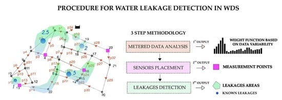
:Many efforts have been made in recent decades to formulate strategies for improving the efficiency of water distribution systems (WDS), led by the socio-demographic evolution of modern society and the climate change scenario. The improvement of WDS management is a complex task that can be addressed by providing services to maximize revenues while ensuring that the quality standards required by national and international regulations are upheld. These two objectives can be fulfilled by utilizing optimized techniques for the operational and maintenance strategies of WDS. This paper proposes a methodology for assisting engineers in identifying water leakages in WDS, thus providing an effective procedure for ensuring high level hydraulic network functionality. The proposed approach is based on an inverse analysis of measured flow rates and pressure data, and consists of three steps: The analysis of measurements to select the most suitable period for leakage identification, the localization of the best measurement points based on a correlation analysis, and leakage identification with a hybrid optimization that combines the exploration capability of the differential evolution algorithm with the rapid convergence of particle swarm optimization. The proposed procedure is validated on a reference hydraulic network, known as the Apulian network.
1. Introduction
The maximization of the efficiency of water distribution systems (WDS) is a topic that is receiving increasing attention from research and industrial institutions due to continuous demographic growth and a worsening of the water crisis [1]. The improvement of WDS has been a challenging task due to a lack of structured and consistent measurement data [2]. However, these systems have been updated recently with advanced data logging systems and intelligent management strategies [3,4,5]. Such actions are aimed not only at increasing the economic profits of water-related services, but also at improving the quality of the service in line with national and international standards. One of the tricky challenges in the management of WDS at the moment is the minimization of water leakages, which represents not only a mass, energy and economical loss, but is also one of the main factors of water contamination [6,7].
Different definitions exist for leakage in water distribution systems. One of the most frequently used defines leakage as the quantity of water which escapes from the pipe network by means other than through a controlled action [8]. Leakages are typically classified into two different categories: Background leakages and bursts. The former are due to water escaping through inadequate joints or cracks, for example, while bursts (i.e., main breaks) represent structural pipe failures [9]. Leaks can also exist in reservoirs and tanks. Leakages in distribution systems can be caused by several factors, such as bad pipe connections, pipe corrosion, and mechanical damage caused by excessive pipe load (e.g., by traffic on the road above, or by a third party working on the system). Other common factors that influence leakages are ground movement, high system pressure, damage due to excavation, pipe age, winter temperature, pipe defects, ground conditions and poor quality of workmanship [8].
The detection of water leakages has usually been undertaken through extensive and expensive on-field operations. Due to the increasing availability of WDS meter data, several efforts have been made to support on-field operation with ex-ante analysis in recent years, and several works have been published on leakage detection and isolation methods for water distribution networks, such as transient-based leak detection methods [10].
Another set of methods is based on inverse transient analysis [11,12,13,14]. The principal concept of this methodology is the analysis of pressure data collected during the occurrence of transitory events by means of the minimization of the difference between the observed and calculated parameters [15].
Pudar and Liggett [16] formulated leak detection as an inverse problem using pressure measurements and defining a sensitivity matrix. This approach, which is used by Pérez et al. [17,18], is based on pressure measurements and leak sensitivity analysis. Leakage localization methods are coupled with hydraulic models to detect leaks and to narrow the area sought. The latter aspect allows focusing investigations into on-site optimal exploration in the areas characterized by a consistent number of leaks.
District audits are labor-intensive and expensive, since they are performed at night. Nowadays, the trend is to install permanent flow meters in the network and connect them telemetrically to a supervisory control and data acquisition (SCADA) system. District audits help identify areas of the network that have excessive leakage but no specific information about the exact location of the leaks is given. It is therefore crucial to know which points of the network are the most representative in order to install the sensor. The selection of the optimal meters positioning, e.g., pressure meters [18,19,20], is addressed in several papers concerning principally the detection of contamination in water distribution networks [21].
The searches for water leaks in WDS, as is generally the case in WDS optimization issues, are mainly based on evolutionary algorithms (EAs) and other metaheuristic techniques. The development and application of these algorithms has been a crucial research field for over the last twenty years, and these techniques are widely used in many different applications, as reported by Maier et al. [22].
In this paper we propose a methodology able to identify water leaks in WDS to support operational engineers and technicians in the preliminary phases of the localization of water leakages.
As first, hours when the WDS was less perturbed were identified and the optimal place to insert a sensor was evaluated through a correlation analysis. Afterwards, the leakages were localized by using a hybrid optimization technique based on differential evolution algorithms and particle swarm optimization. All the analyses were carried out on the Apulian network.
This paper is organized as follows: Introduction of the methodology for both sensor placement and leakages detection, summary of the results, and presentation of conclusions.
2. Methodology
The goal of this study is to localize the position of an imposed leakage in a well-known network through an inverse analysis, taking into account the flow rate delivery by the reservoir, and pressures measured at specific points in the network.
To do this, a hybrid evolutive algorithm [23] was used to localize and identify the magnitude of the leakages into WDS. This algorithm combines the large exploration capability of differential evolution (DE) and the fast convergence of particle swarm optimization (PSO), so it is called “differential evolutive particle swarm optimization” (DEPSO).
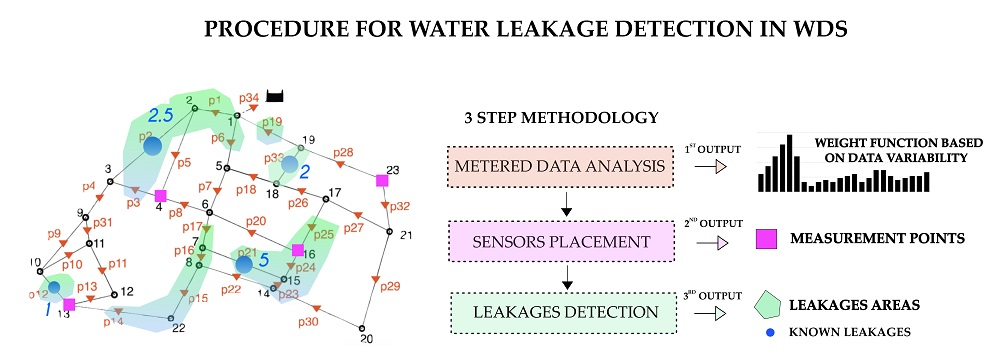
The proposed methodology was tested and validated on the Apulian network [24] which is a synthetic network consisting of 34 pipes, 23 users, and 1 reservoir (Figure 1).
Each user node was suitable for the insertion of a flow meter while emitter nodes were placed in the middle of each pipe of the network in order to evaluate pipe leakages. The location and the amount of fictitious leakages are shown in Figure 1 through the large circles and the corresponding value, which were chosen according to Debiasi et al. [25]. In order to minimize error in the inverse analysis and to make this analysis consistent with a real case study, the hours in which the WDS presented a minor perturbation were identified (i.e., when the system had a maximum sensitivity to losses), and the best location for placing a sensor was investigated.
2.1. Characterization of the Demand Pattern
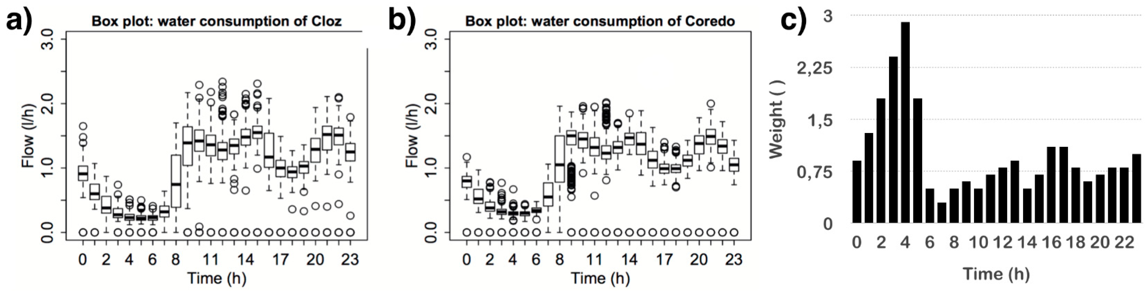
The real data of water consumptions in two small municipalities in the Trentino-Alto Adige region of Italy were analyzed. We were then able to build the demand pattern of the Apulian network by analyzing the data measured in real cases. In fact, the hourly pattern used in the Apulian network was the average of the two municipalities’ demand behavior, and the resulting weight function was adopted for leak detection.
Figure 2a,b show the statistics of hourly consumptions recorded during a year of measurements. The demand and pressure of the two networks were analyzed to identify the more suitable hours for the inverse analysis of leak detection. The hours characterized by a high variability of water demand were not sufficiently stable or representative of the global behavior of the WDS, so low importance was associated to such hours, which were usually daytime hours. On the contrary, higher weights were assigned to the night time hours, which were characterized by limited variability. Figure 2c shows the weight associated to each hour, calculated as the inverse of the correspondent water demand variance.
2.2. Measurement Points Identification
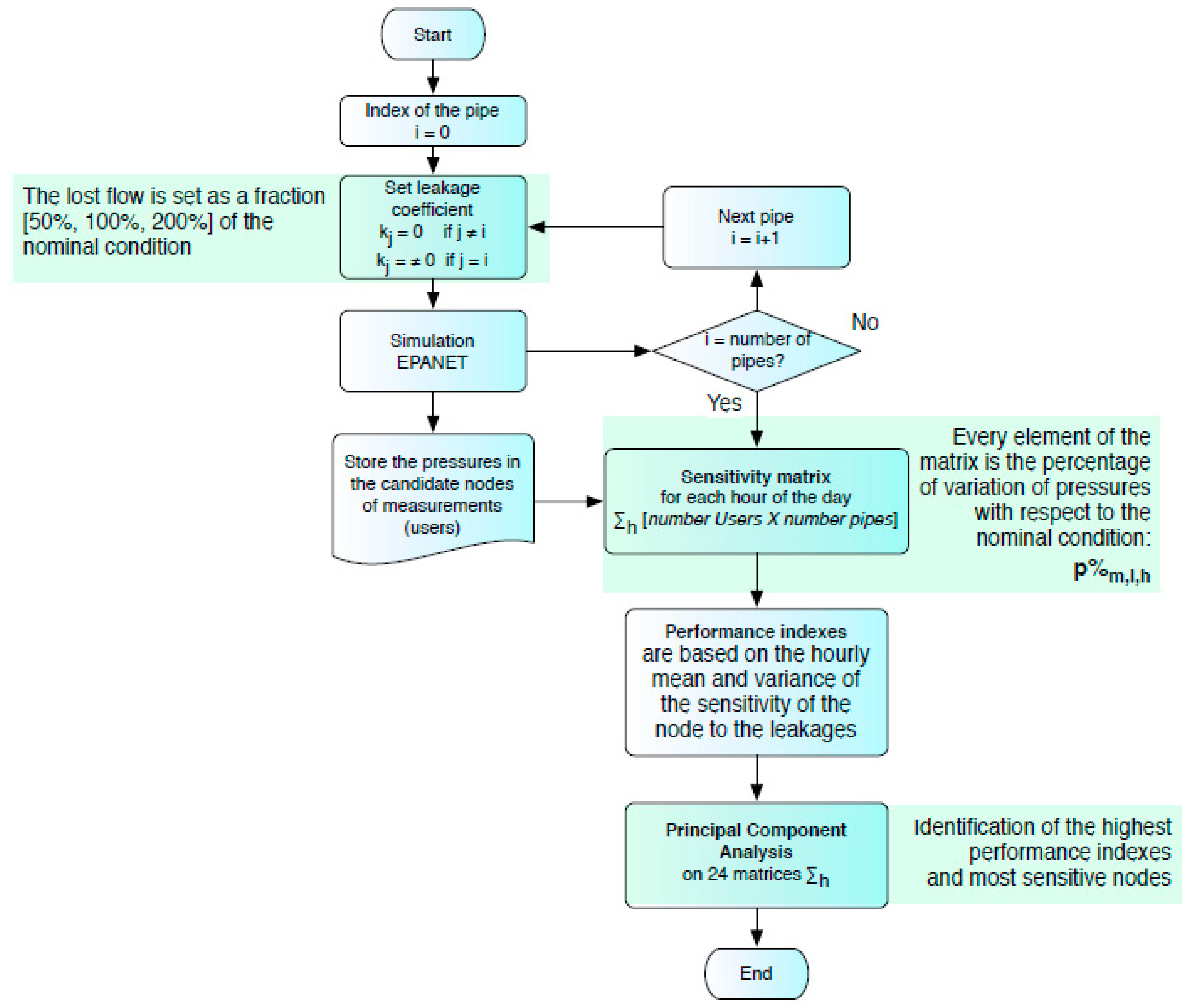
Since the number of sensors that can be displaced in a real network is limited, it is important to place them in optimal locations. In this study, during the identification of the best measurement points, it is assumed that only four pressure sensors are usable in the WDS. The challenge was to select the four measurement nodes (users) that both maximize the sensitivity of the pressure meters with respect to the leakages, and provide uncorrelated measurements. These two requirements were fulfilled by a sensitivity analysis and a subsequent correlation analysis of the WDS. To this aim, the procedure followed the approach developed by Bort et al. [19], as shown in the algorithm scheme in Figure 3.
This methodology was based on two stages. The first analysis related to the sensitivity analysis of the user nodes at leakages. A sensitivity matrix was calculated for each hour of the day, by placing a known leakage into one pipe and recording the pressure measured on every user node. The leaking flow was set as a ratio of the nominal flow (where no leakages are placed into the network). Three ratios were tested: 0.5, 1, and 2, in order to consider the effect of the leakage magnitude. The emitter coefficient was calculated from the imposed leaking flow as follows:
where is the pressure, and is the pressure exponent set to 0.5. The sensitivity matrix relative to the -th hour is called and it has as many rows as the number of user nodes (i.e., 23), and as many columns as the number of pipe nodes (i.e., 34). Each element of the 24 sensitivity matrices was called , and this represents the percentage of variation of the pressure at the measurement node with respect to the nominal case when a leakage was placed into the pipe and the measurement was carried out at hour .
Suitable performance indexes are defined on each element of the matrix in order to reduce the dimensions of the 24 matrices to four values for user nodes [19]. The four indexes are as follows:
1. The mean of the mean percentage pressure variations across different positions of the leaking pipe . These quantities are calculated as:
2. The variance of across the day:
3. The mean across the whole day of , that is defined as the variance of across the different position of the leakages:
4. The variance across the whole day of :
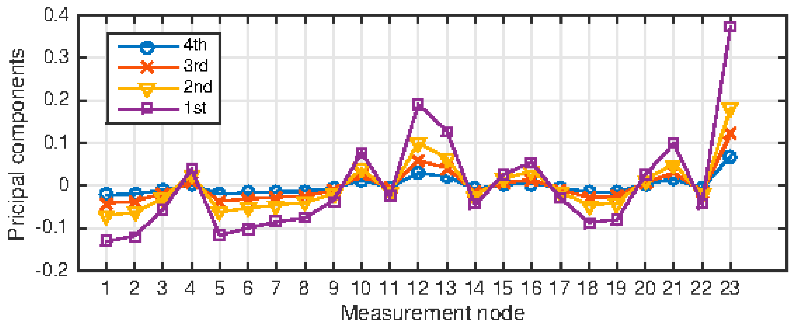
Once the four features were calculated, a principal component analysis (PCA) was carried out in order to extract the most sensitive from between -nodes. Figure 4 shows the principal component analysis carried out on the sensitivity study results.
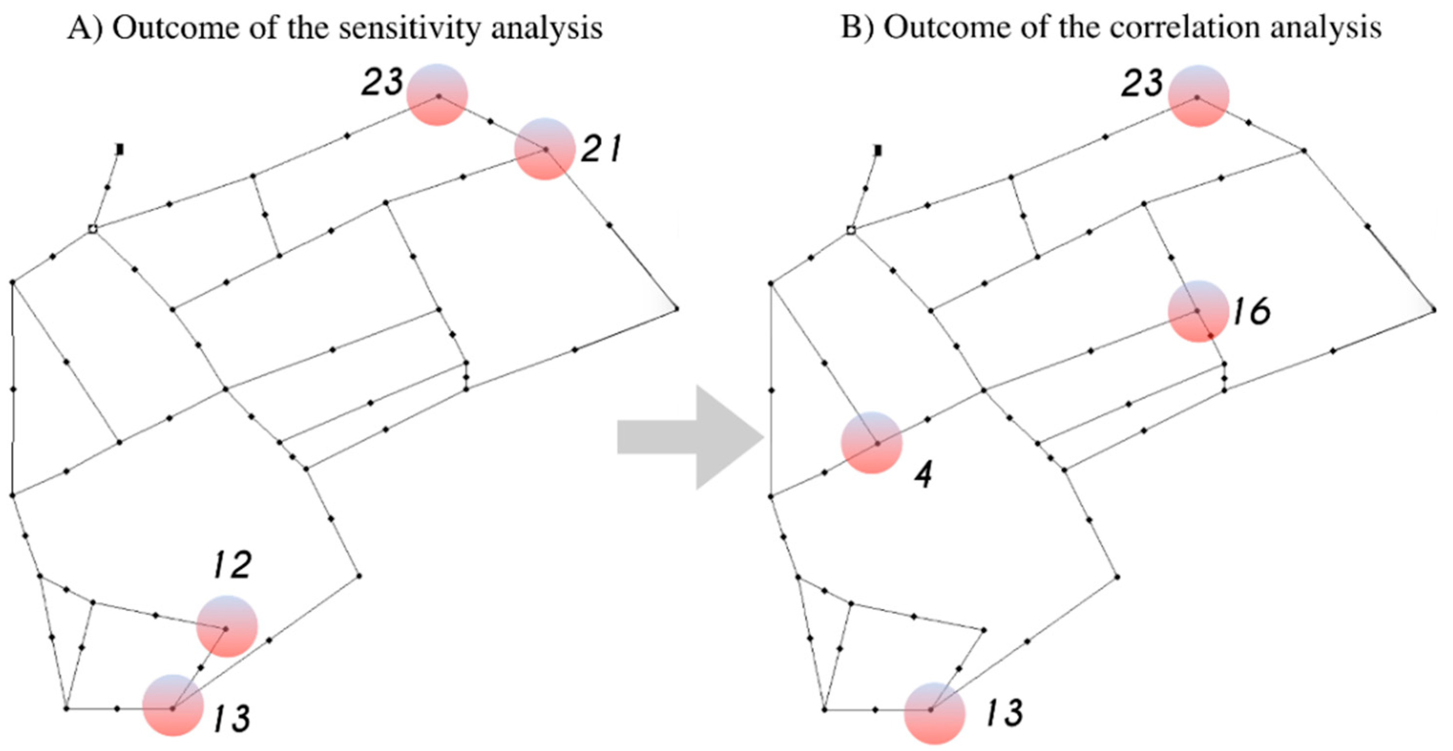
By definition of the calculated features, only the positive principal components were associated to a decreasing in the measurement pressure due to a leaking pipe. For such a reason, the negative values of principal components were neglected and rounded to zero. The four most sensitive measurement nodes found from this analysis were numbers 23, 12, 13, and 21. Figure 5A shows that these sensitive nodes are close to each other, therefore, redundant information was used for the inverse analysis if the pressure sensors were placed on the most sensitive nodes.
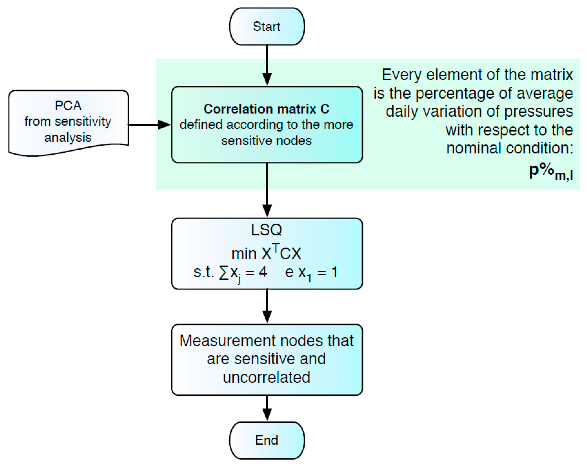
The second stage aimed to overcome this limitation through a correlation analysis, following the scheme in Figure 6. The percentage variations of the measured pressure with respect to the non-leaking cases were averaged across the hours of the day, thus obtaining a matrix P whose elements were the daily average of percentage of the pressure variations. According to the considerations made from the previous PCA analysis, all the rows of associated to nodes with negative principal components were neglected. Therefore, the matrix is reduced to a dimension . The correlation matrix was defined as:
The most uncorrelated points were obtained by solving a least square optimisation (LSQ), that was defined as:
where is a vector with 9 elements, in which the -th element is associated to the candidate measurement node with the -th 1st PCA component. The following constraints were associated with the target function:
• The -th element of was close to 1 if it was uncorrelated from other nodes (it will host a pressure sensor), 0 otherwise:
• The node 23, that is the most sensitive measurement node, was always taken as a measurement node:
The outcome of this analysis was the four nodes 23, 16, 13, and 4, which were not only sensible to the position of leakages in the network, but also uncorrelated from each other. The position of these four measurement nodes is shown in Figure 5B.
2.3. Leakage Detection
The inverse analysis for the leak detection was formulated as an optimization problem. The emitter coefficients of all pipes nodes were calibrated until the pressures of the four selected measurement nodes and the flow rate supplied by the reservoir simulated by the widely used hydraulic simulator EPANET [26] matched the pressures and flow rate measured. The latter is the theoretical Apulian network in which four leakages were imposed according to Figure 1. The formulation of the optimization problem is shown by the following equation:
where is the vector of emitter coefficient, are the hourly weights calculated from step 1 (Figure 2c), is the pressure simulated at the -th measurement node and recorded at -th hour (note the dependency of the pressure from the value of the emitter coefficients ), is the simulated water flow leaving the reservoir relative to the -th hour, while and are the reference pressure at measurement nodes and flow rate respectively. Note that it is assumed that only four nodes in the network were leaking since the pressure was measured on only four nodes, otherwise the optimisation problem would be ill-conditioned.
Three constraints are applied to the target function. Sources of uncertainty on the moder of the hydraulic network were taken into account by accepting that the global emitter could vary up to 10%:
Each emitter coefficient was constrained to be positive, but limited to a maximum value. The upper limit was set by assuming that in the worst case the total leakage of the network was concentrated in one node. Such a condition corresponds to a maximum emitter coefficient :
The complete target function is obtained by combining Equation (12) with Equations (13)–(15):
The optimization algorithm used for minimizing the target function in Equation (16) was the differential evolution particle swarm (DEPSO), which is a hybrid evolutive algorithm in which a population (i.e., a group) of individuals (i.e., candidate set of emitter coefficients) is evolved until the target function is minimized. Each population had 50 individuals, and each individual was a set of 8 variables. The first four elements of an individual defined the number of the four leaking nodes (the number of leaking nodes matches the number of nodes in which pressure was measured in order to avoid ill-conditioned problems), while the remaining four elements defined the emitter coefficient of each leakage.
The individuals of the first population were generated by randomly sampling the emitter coefficients from a uniform distribution. The evolution then proceeded by alternating an iteration with the differential evolution (DE) [27] with an iteration with the particle swarm optimization (PSO). At the k-th iteration step, each individual of the population was updated with the best population , which was the population grouping of the best individuals calculated during the whole optimization process. The values of the target functions relative to the elements in are stored into .
Then, the mutation operation was performed according to a random scheme. Three array of indexes , , and were randomly generated from a uniform distribution, and with as many elements as individuals in the population (that in this study is 66). The population was given by:
where the scaling factor is equal to 0.6 (this value has been chosen after a manual calibration).
The cross-over operation was applied to with a probability of 60%. For each -th individual in , a vector was produced of 8 randomly generated numbers sampled from a uniform distribution defined in the interval . The indexes corresponding to the elements of identify which elements of were replaced with the correspondent elements of the individual and .
At the end of the cross-over step, a new population was obtained and the target function was evaluated for each individual of . The DE step ended by creating a population assembled by merging the best individuals of and .
At this point it was applied a PSO step to , according to the algorithm proposed in Clerc & Kennedy [28]. It is defined a constriction factor :
where is the social acceleration coefficient and is the cognitive acceleration coefficient. The values of the two parameters were selected as suggested in the literature [29] and by assuring that .
Then the velocities of each -th individual in were updated:
is the best individual in the population, while and represent uniform random numbers between 0 and 1. The velocities were used to update the current population:
The target function was evaluated for each individual in , and the relative values of the target function were stored in . The optimisation was stopped if the difference between the maximum and minimum values in was less than , or after iterations. Otherwise, the next iteration was performed starting again from step 1.
3. Results
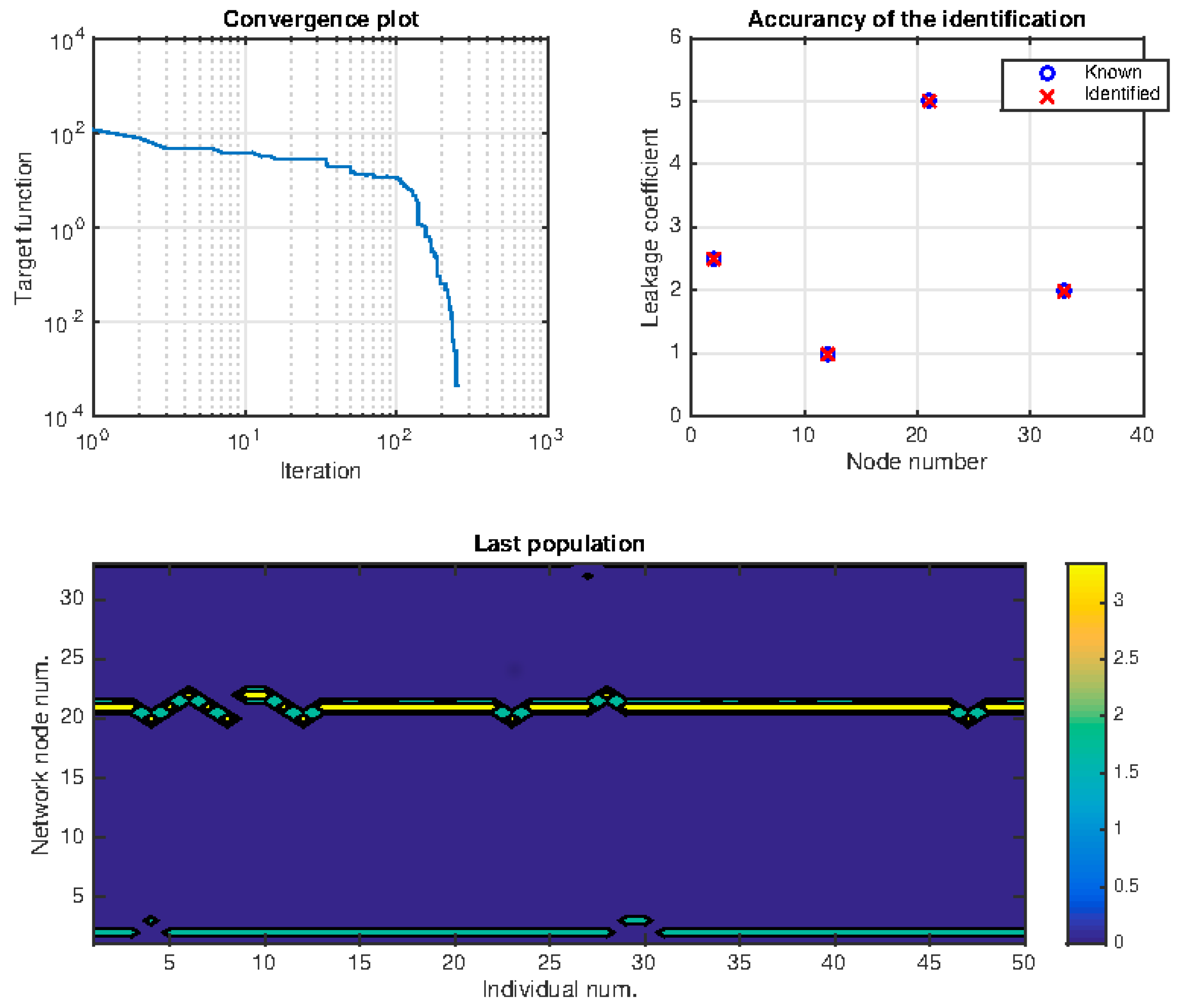
In order to take into account the intrinsic stochasticity of evolutive algorithms, the identification was performed 10 times. The best result of the 10 identifications is shown in Figure 7. On the top left the convergence plot is shown on a logarithmic scale. Convergence was reached after 253 iterations. The best set of emitter coefficients is shown on the top right and it is compared to the a-priori imposed leakages. It is possible to observe how the identified leakages match not only their position, but also their nominal values.
Emitter coefficients across the best population are shown in the lower panel: The abscissa shows the individuals, and the ordinate shows the number of leaking pipes, while color is associated with the magnitude of the emitter coefficient. This colored diagram shows the stability of the identified solution: Horizontal streams of colors indicate that a given pipe number was recognized as leaking for multiple individuals in the population. Due to the intrinsic stochasticity behind the DEPSO optimization algorithm, emitter coefficients, that were more frequent across the individuals of the population, were more likely be closer to the exact solution.
The performance of the proposed methodology was strongly dependent on the initial guest provided to the DEPSO algorithm. In order to achieve a robust identification, increasing the number of identification trials while reducing the number of iterations was recommended. By doing this, the exploration of a large space of the optimization domain was guaranteed.
4. Conclusions
A methodology suitable for supporting technicians and engineers in locating and quantifying leakages in a water distribution system has been proposed. The suggested methodology was based on three innovative concepts: A statistical analysis of water consumption, a sensitive and correlation analysis, and an inverse identification through a hybrid evolutive optimization algorithm.
The statistical study of water consumption trends during a one-year period allowed us to determine the hours of the day that were characterized by more repeatable consumption patterns, which could therefore provide accurate measurements. Such an approach extends the applicability of the proposed procedure to a wide category of WDS, even characterized by intermittent water consumptions. The sensitivity and correlation analyses of the hydraulic network suggested which the optimal nodes of the network were, and where to install pressure sensors, suitable for the health monitoring of the WDS. Finally, the inverse identification attempted to reconstruct the set of emitter coefficients (i.e., leakages) that generated the measured pressures.
The proposed approach was validated by a theoretical network that is characterized by the complete knowledge of topological and hydraulic properties.
The network was monitored by four pressure sensors which were strategically located, and the leakages were estimated to be half way along four pipes. The result of the inverse optimization shows that with a reduced number of pressure sensors it is possible to estimate the position of the leakages on a restricted subset of pipes in the network. Due to the stochasticity of evolutive algorithms, multiple identifications had to be run in order to achieve a robust solution. However, each identification needed to be run for a low number of iterations since the initial guest appeared to be the major factor in finding the global optimum. It had to be mentioned, moreover, that the procedure was carried out on a low-power personal computer, and this could have been overcome by exploiting parallelized implementations of the DEPSO algorithm to be executed on distributed processors, such as on graphical processing units (GPU).
Finally, it should be mentioned that one of the advantages of the proposed approach is that it is scalable. Large WDSs can be sectioned into smaller WDS if the boundary conditions are set properly (e.g., by monitoring the nodes at the frontier of the sub-WDS with pressure and flow sensors).
Author Contributions
Conceptualization, M.R., A.M., A.Z., C.M.G.B. and M.B.; Methodology, M.R., A.M., A.Z., C.M.G.B. and M.B.; Software, C.M.G.B. and M.B.; Writing—Original Draft Preparation, A.M., C.M.G.B. and M.B.; Writing—Review & Editing, A.M., A.Z., and M.B.; Supervision, M.R.; Funding Acquisition, M.R.
Funding
This research was funded by the EFRE-FESR project: “Thermo Fluid Dynamics, infrastructures for applied research” (ERDF 2014-2020, CUP: I52F16000850005) and by the Research project “AI-ALPEN: Supply of drinking water in alpine regions”, (third call for Research projects founded by Autonomy Provence of Bozen/Bolzano-Italy, CUP: B26J16000300003).
Conflicts of Interest
The authors declare no conflicts of interest.
References
- Jakob, M.; Steckel, J.C. Implications of climate change mitigation for sustainable development. Environ. Res. Lett. 2016, 11, 104010. [Google Scholar] [CrossRef] [Green Version]
- Gargano, R.; Tricarico, C.; Granata, F.; Santopietro, S.; de Marinis, G. Probabilistic models for the peak residential water demand. Water 2017, 9, 417. [Google Scholar] [CrossRef]
- Di Nardo, A.; di Natale, M.; Giudicianni, C.; Santonastaso, G.F.; Tzatchkov, V.; Varela, J.M.R. Economic and energy criteria for district meter areas design of water distribution networks. Water 2017, 9, 463. [Google Scholar] [CrossRef]
- Carravetta, A.; Del Giudice, G.; Fecarotta, O.; Ramos, H.M. Pump as turbine (PAT) design in water distribution network by system effectiveness. Water 2013, 5, 1211–1225. [Google Scholar] [CrossRef]
- Brentan, B.; Meirelles, G.; Luvizotto, E.; Izquierdo, J. Joint Operation of Pressure-Reducing Valves and Pumps for Improving the Efficiency of Water Distribution Systems. J. Water Resour. Plan. Manag. 2018, 144, 04018055. [Google Scholar] [CrossRef]
- Abd Rahman, N.; Muhammad, N.S.; Wan Mohtar, W.H.M. Evolution of research on water leakage control strategies: Where are we now? Urban Water J. 2018, 15, 812–826. [Google Scholar] [CrossRef]
- Federici, E.; Meniconi, S.; Ceci, E.; Mazzetti, E.; Casagrande, C.; Montalbani, E.; Businelli, S.; Mariani, T.; Mugnaioli, P.; Cenci, G.; et al. Legionella survey in the plumbing system of a sparse academic campus: A case study at the University of Perugia. Water 2017, 9, 662. [Google Scholar] [CrossRef]
- Puust, R.; Kapelan, Z.; Savic, D.A.; Koppel, T. A review of methods for leakage management in pipe networks. Urban Water J. 2010, 7, 25–45. [Google Scholar] [CrossRef]
- O’Day, D.K. Organization and analyzing leak and break data for making main replacement decisions. J. Am. Water Work. Assoc. 1982, 74, 588–594. [Google Scholar] [CrossRef]
- Colombo, A.F.; Lee, P.; Karney, B.W. A selective literature review of transient-based leak detection methods. J. Hydro-Environ. Res. 2009, 2, 212–227. [Google Scholar] [CrossRef]
- Ferrante, M.; Brunone, B. Pipe system diagnosis and leak detection by unsteady-state tests. 1. Harmonic analysis. Adv. Water Resour. 2003, 26, 95–105. [Google Scholar] [CrossRef]
- Ferrante, M.; Brunone, B. Pipe system diagnosis and leak detection by unsteady-state tests. 2. Wavelet analysis. Adv. Water Resour. 2003, 26, 107–116. [Google Scholar] [CrossRef]
- Soares, A.K.; Covas, D.I.C.; Reis, L.F.R. Leak detection by inverse transient analysis in an experimental PVC pipe system. J. Hydroinform. 2011, 13, 153–166. [Google Scholar] [CrossRef]
- Covas, D.; Ramos, H. Hydraulic transients used for leakage detection in water distribution systems. In Proceedings of the 4th International Conferene on Water Pipeline Systems, York, UK, 28–30 March 2001. [Google Scholar]
- Perez, R.; Sanz, G.; Puig, V.; Quevedo, J.; Escofet, M.A.C.; Nejjari, F.; Meseguer, J.; Cembrano, G.; Tur, J.M.M.; Sarrate, R. Leak localization in water networks: A model-based methodology using pressure sensors applied to a real network in Barcelona [applications of control]. IEEE Control Syst. 2014, 34, 24–36. [Google Scholar]
- Pudar, R.S.; Liggett, J.A. Leaks in pipe networks. J. Hydraul. Eng. 1992, 118, 1031–1046. [Google Scholar] [CrossRef]
- Pérez, R.; Puig, V.; Pascual, J.; Peralta, A.; Landeros, E.; Jordanas, L. Pressure sensor distribution for leak detection in Barcelona water distribution network. Water Sci. Technol. Water Supply 2009, 9, 715–721. [Google Scholar] [CrossRef]
- Pérez, R.; Puig, V.; Pascual, J.; Quevedo, J.; Landeros, E.; Peralta, A. Methodology for leakage isolation using pressure sensitivity analysis in water distribution networks. Control Eng. Pract. 2011, 19, 1157–1167. [Google Scholar] [CrossRef] [Green Version]
- Bort, C.M.G.; Righetti, M.; Bertola, P. Methodology for Leakage Isolation Using Pressure Sensitivity and Correlation Analysis in Water Distribution Systems. Procedia Eng. 2014, 89, 1561–1568. [Google Scholar] [CrossRef] [Green Version]
- Lima, G.M.; Brentan, B.M.; Manzi, D.; Luvizotto, E. Metamodel for nodal pressure estimation at near real-time in water distribution systems using artificial neural networks. J. Hydroinform. 2018, 20, 486–496. [Google Scholar] [CrossRef]
- Rathi, S.; Gupta, R. Sensor Placement Methods for Contamination Detection in Water Distribution Networks: A Review. Procedia Eng. 2014, 89, 181–188. [Google Scholar] [CrossRef] [Green Version]
- Maier, H.R.; Kapelan, Z.; Kasprzyk, J.; Kollat, J.; Matott, L.S.; Cunha, M.C.; Dandy, G.C.; Gibbs, M.S.; Keedwell, E.; Marchi, A.; et al. Evolutionary algorithms and other metaheuristics in water resources: Current status, research challenges and future directions. Environ. Model. Softw. 2014, 62, 271–299. [Google Scholar] [CrossRef] [Green Version]
- Zhang, W.-J.; Xie, X.-F. DEPSO: Hybrid particle swarm with differential evolution operator. In Proceedings of the 2003 IEEE International Conference on Systems, Man and Cybernetics, Washington, DC, USA, 5–8 October 2003; Volume 4, pp. 3816–3821. [Google Scholar]
- Giustolisi, O.; Savic, D.; Kapelan, Z. Pressure-Driven Demand and Leakage Simulation for Water Distribution Networks. J. Hydraul. Eng. 2008, 134, 626–635. [Google Scholar] [CrossRef] [Green Version]
- Debiasi, S.; Bort, C.M.G.; Bosoni, A.; Bertola, P.; Righetti, M. Influence of Hourly Water Consumption in Model Calibration for Leakage Detection in a WDS. Procedia Eng. 2014, 70, 467–476. [Google Scholar] [CrossRef] [Green Version]
- Rossman, L.A. EPANET 2: Users Manual; U.S. Environmental Protection Agency: Washington, DC, USA, 2000.
- Das, S.; Abraham, A.; Chakraborty, U.K.; Konar, A. Differential Evolution Using a Neighborhood-Based Mutation Operator. Trans. Evol. Comput. 2009, 13, 529–553. [Google Scholar] [CrossRef]
- Clerc, M.; Kennedy, J. The particle swarm—Explosion, stability, and convergence in a multidimensional complex space. IEEE Trans. Evol. Comput. 2002, 6, 58–73. [Google Scholar] [CrossRef]
- Schutte, J.F.; Groenwold, A.A. A Study of Global Optimization Using Particle Swarms. J. Glob. Optim. 2005, 31, 93–108. [Google Scholar] [CrossRef] [Green Version]
Figure 1.
Apulian network layout with the leaking nodes and the correspondent emitter coefficients highlight in red.
Figure 1.
Apulian network layout with the leaking nodes and the correspondent emitter coefficients highlight in red.

Figure 2.
Box plots of hourly water consumptions (l/h) of the two Italian municipalities: Cloz (a) and Coredo (b). Weights (adimensional) are used for the definition of the target function (c).
Figure 2.
Box plots of hourly water consumptions (l/h) of the two Italian municipalities: Cloz (a) and Coredo (b). Weights (adimensional) are used for the definition of the target function (c).

Figure 3.
Algorithm scheme of the sensitivity analysis.

Figure 4.
Principal components calculated for each measurement node.

Figure 5.
Results of the sensitivity (A) and correlation (B) analysis.

Figure 6.
Algorithm scheme of the correlation analysis.

Figure 7.
Convergence plot of the differential evolutive particle swarm optimization (DEPSO)-based optimization (top left panel), identified emitter coefficients and reference values of known leakages (top right panel), values of emitter coefficients across the last population (lower panel).
Figure 7.
Convergence plot of the differential evolutive particle swarm optimization (DEPSO)-based optimization (top left panel), identified emitter coefficients and reference values of known leakages (top right panel), values of emitter coefficients across the last population (lower panel).

© 2019 by the authors. Licensee MDPI, Basel, Switzerland. This article is an open access article distributed under the terms and conditions of the Creative Commons Attribution (CC BY) license (http://creativecommons.org/licenses/by/4.0/).
Share and Cite
MDPI and ACS Style
Righetti, M.; Bort, C.M.G.; Bottazzi, M.; Menapace, A.; Zanfei, A. Optimal Selection and Monitoring of Nodes Aimed at Supporting Leakages Identification in WDS. Water 2019, 11, 629. https://doi.org/10.3390/w11030629
AMA Style
Righetti M, Bort CMG, Bottazzi M, Menapace A, Zanfei A. Optimal Selection and Monitoring of Nodes Aimed at Supporting Leakages Identification in WDS. Water. 2019; 11(3):629. https://doi.org/10.3390/w11030629
Chicago/Turabian StyleRighetti, Maurizio, Carlos Maximiliano Giorgio Bort, Michele Bottazzi, Andrea Menapace, and Ariele Zanfei. 2019. "Optimal Selection and Monitoring of Nodes Aimed at Supporting Leakages Identification in WDS" Water 11, no. 3: 629. https://doi.org/10.3390/w11030629
Note that from the first issue of 2016, this journal uses article numbers instead of page numbers. See further details here.