A Comparison of Continuous and Event-Based Rainfall–Runoff (RR) Modelling Using EPA-SWMM

School of Natural and Built Environments, University of South Australia, Mawson Lakes 5095, Australia
*
Author to whom correspondence should be addressed.
Water 2019, 11(3), 611; https://doi.org/10.3390/w11030611
Submission received: 11 December 2018
/
Revised: 18 March 2019
/
Accepted: 21 March 2019
/
Published: 24 March 2019
(This article belongs to the Special Issue Catchment Modelling)
Abstract
:This study investigates the comparative performance of event-based and continuous simulation modelling of a stormwater management model (EPA-SWMM) in calculating total runoff hydrographs and direct runoff hydrographs. Myponga upstream and Scott Creek catchments in South Australia were selected as the case study catchments and model performance was assessed using a total of 36 streamflow events from the period of 2001 to 2004. Goodness-of-fit of the EPA-SWMM models developed using automatic calibration were assessed using eight goodness-of-fit measures including Nash–Sutcliff efficiency (NSE), NSE of daily high flows (ANSE), Kling–Gupta efficiency (KGE), etc. The results of this study suggest that event-based modelling of EPA-SWMM outperforms the continuous simulation approach in producing both total runoff hydrograph (TRH) and direct runoff hydrograph (DRH).
1. Introduction
Rainfall–runoff (RR) models are important tools for planning, design and management of water resource systems. These models are used in a wide range of hydrological applications ranging from the estimation of catchment runoff to analyzing the impact of land-use change on runoff [1]. The methods of synthesizing the rainfall–runoff process in these models differ from one model to another, consequently a variety of model classifications exist. According to Brocca et al. [2], RR models can be classified based on their spatial structure (lumped versus semi-distributed or distributed), time representation (continuous time versus event-based) or process description (physically meaningful versus data-driven). Daniel et al. [3] adopted four different classifications for RR models based on: (i) parameter specification (deterministic or stochastic); (ii) the nature of the basic algorithms (empirical, conceptual or physically-based); (iii) spatial representation (lumped, semi-distributed or distributed); and (iv) the temporal representation (event-based or continuous time). Similar classifications can be found in Elga et al. [4], Singh [5] and Wheater et al. [6]. Of the available models, spatial and temporal representations are the most commonly adopted model types [7,8], while event-based (EB) and continuous simulation (CS) models are the most recognized category within the temporal domain [4,5]. In EB modelling, the rainfall–runoff process in a catchment is simulated for a single rainfall or streamflow event with durations ranging from several hours to several days. Whereas in CS modelling the rainfall–runoff process is simulated for a long time period ranging from a couple of months to several years, including both dry and wet seasons. Generally, in EB modelling, only the infiltration process is modelled in order to account for losses, while in CS modelling, the evapotranspiration loss is also accounted for [9].
CS and EB models both have advantages and limitations. One major advantage of CS modelling is that it is capable of accounting for antecedent conditions such as initial soil-moisture status, stream and reservoir level, water table depth, etc. [10,11]. In contrast, EB models are unable to account for antecedent conditions, instead values are subjectively assigned by the user and then calibrated using an observed hydrograph [12,13]. The great disadvantage of CS modelling is that it requires a long period of hydrological observations making its application challenging in case of a limited data availability [14,15]. EB modelling offers more flexibility in this case as it does not require a long period of hydrological data [14,16].
Catchment urbanization, land-use and land-cover are some dominant factors affecting the performance of RR modelling [1,14,15,17]. Hydrological processes can greatly alter due to land use change and therefore runoff generation process in a rural catchment is different to that of an urban catchment. [14,15,16,17]. In rural catchments, runoff patterns and paths on the soil surface evolve from natural conditions such as topography and land use, whereas in urbanized catchments, flow paths are mainly predefined by the sewer and stormwater management system and hence the runoff is not obstructed by any significant retention process [14,15,18]. Hydrographs generated from urban catchments are more likely to have spikey shapes because during a storm event runoff reaches a peak quickly by following the sewerage path and falls quickly, once rainfall ceases [1,15]. On the other hand, streamflow hydrographs generated in rural catchments are more likely to have gentle shapes, with streamflows peaking relatively slowly during a storm event and falling gradually over a long period after the storm is over [15,17]. Generally, rural catchments are dominated by pervious surfaces with a wide range of vegetation cover and hence, are subject to more substantial runoff losses and flow peaks are delayed [1,14,16,17]. On the other hand, urban catchments are dominated by impervious areas that are directly connected to the sewerage or stormwater systems, thereby resulting in a quick peak during a storm event. Therefore, depending on the catchment condition, there is a clear distinction between hydrographs generated by urban and rural catchments, consequently the performance of EB and CS models can vary from one catchment to another.
Many researchers have found that an EB approach performed better than the CS approach for their case study catchments. For example, Chu et al. [8] compared continuous and EB approaches on Mona Lake Watershed in West Michigan and obtained a better fit using an EB model. Similarly, De Silva et al. [19] studied the hydrology of the Kelani River basin in Sri Lanka and found that the EB model performed better when simulating extreme events. Sampath et al. [20] used continuous and EB approaches to predict streamflow hydrographs from Tittawella tank catchment in Sri Lanka and found that the EB model performed better over the relatively short study period. Azmat et al. [21] studied a high-altitude watershed using continuous and EB modelling and found the EB model was more accurate. In contrast, Cunderlik and Simonovic [22] found that CS was able to produce more reliable hydrographs. In the recent review of ARR 2016 (Australian rainfall–runoff) [16], CS model is reported to have limited ability to represent rural catchment behavior, which contrasts with other researchers including Brocca et al. [2], Boughton and Droop [23], Paquet et al. [24], who have successfully used the CS approach to estimate design floods and carry out real time flood forecasting. Furthermore, Kemp and Hewa [25] have recently found that EB modelling performed by RORB (run-off routing burroughs) [12], as recommended by ARR 2016, was unable to produce reliable flood quantiles at more frequent events. Therefore, it is both timely and important to explore the ability of EB and CS modelling approaches to accurately estimate runoff hydrographs and design floods resulting from more frequent events. The focus of the above cited studies has been to assess the performance of EB and CS modelling in reproducing the observed streamflow hydrograph (also known as total runoff hydrograph), while the current study considered both total runoff hydrograph (TRH) as well as direct runoff hydrograph (DRH).
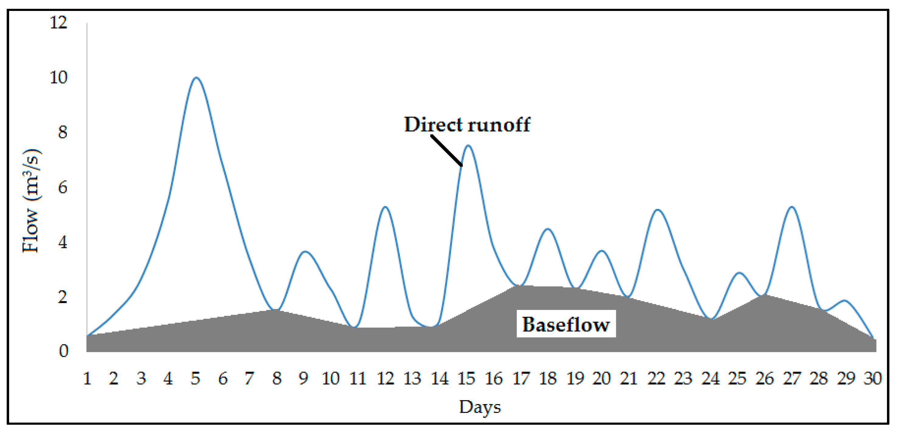
The DRH is the hydrograph that remains after removing baseflow from the TRH. Baseflow represents the usual day to day flow that appears in a stream because of groundwater seepage. The separation of baseflow from the total hydrograph is an inexact science because the direct runoff and baseflow are distinct processes and are partially interrelated [26,27,28]. However, various graphical and filtering techniques have been developed to perform baseflow separation (see Section 2.5 for details) [28,29,30,31,32,33]. The study of DRHs is important in order to understand the influence of the various hydrological processes that govern flow generation from a catchment [26] and because the timing, duration and magnitude of groundwater flows is quite distinct from that of direct runoff [27], understanding these distinct processes is the key to identifying the likely hydrologic response characteristics of a catchment [34].
Nowadays, several computer-based RR modelling tools have been developed that frequently used in hydrological studies across worldwide. Among them, RORB [12], WBNM (watershed bounded network model) [35], RAFTS (runoff analysis and flow training simulation) [36] and ILSAX [37] are EB modelling tools commonly used in Australia. In contrast, some RR modelling tools have been developed that can conduct both EB and CS modelling. Examples of widely used such modelling tools include: HEC-HMS (RR model developed by US Army Corp of Engineers-Hydrologic Engineering Centre) [38], PRMS (precipitation-runoff modelling system developed by U.S. Geological Survey) [39], EPA-SWMM (storm water management model developed by the Environmental Protection Agency, USA) [11,40,41,42,43], AWBM (Australian water balance model) [44], XP-SWMM (storm water management model developed by XP Software Inc.).
While each modelling tool has its own strengths and weaknesses, EPA-SWMM is a catchment scale model capable of simulating single events as well as continuous time series, water quality, storage and treatment, in both urban and rural catchments [11,41]. This model is available in the public domain and has been successfully applied across a wide range of geographical areas [10,45,46,47] and because of its high potentiality, this model is widely adopted in Australian context for hydrological studies [15,48,49]. For instance, Wella-Hewage [15] used the EPA-SWMM model to assess the performance of water-sensitive urban design (WSUD) systems for greenfield catchments in South Australia. Choi and Ball [48] used the EPA-SWMM model to study the runoff characteristics of Centennial Park catchments in Sydney in order to develop a more efficient parameter estimation methodology for urban catchments. Chowdhury et al. [49] also used the EPA-SWMM model to run a series of stormwater harvesting and urbanization scenarios on a number of catchments located in southeast Queensland. Hence, it is evident that EPA-SWMM can be used in a wide range of hydrological applications and therefore, it is a suitable modelling tool for assessing the performance of EB and CS modelling.
The aim of this study is to explore the ability of EB and CS modelling approaches to accurately estimate runoff hydrographs and design floods resulting from more frequent events in semi-rural catchments in a semi-arid environment. More specifically the study explores the ability of the models to accurately reproduce both the TRH and the DRH. The outcomes of this study will act as a decision-making tool in areas including but not limited to: (i) the understanding of the hydrologic response of these types of catchments; (ii) design flood estimation; and (iii) further planning and development. Considering the capabilities of EPA-SWMM, its publicly availability and wider acceptance in Australian context, this modelling tool will be adopted for this investigation.
This paper presents the details of the investigation and its outcome in the following order: (i) a description of the study catchments; (ii) EPA-SEMM model architecture; (iii) data used in the study; (iv) model setup, calibration and validation procedure; (v) results and discussion; and (vi) summary of the findings, modelling assumptions, limitations and conclusions.
2. Materials and Methods
2.1. Study Area
For this study, several South Australian catchments were initially considered and finally two catchments: Myponga upstream and Scott Creek were selected as case study catchments based on the fact that rain gauges are located in close proximity to these catchments and data for these gauges are readily available. Besides, these catchments have been frequently used in hydrological, hydrogeological and climate change studies. For instance, the Myponga upstream catchment has been used for hydrological studies by Wella-Hewage [15], Akhter and Hewa [17] and climate change studies by Jones et al. [50]. Similarly, Scott Creek catchment has been used for hydrogeological studies by Banks et al. [51], Bestland et al. [52] and climate change studies by Ward et al. [53]. Moreover, these catchments have distinctive hydrogeological characteristics and therefore RR modelling performance can vary markedly [15,51,54].
The Myponga upstream catchment is located about 50 km south of the city of Adelaide. The whole catchment covers an area of 122 km2 while upstream and downstream areas covering 73 km2 and 49 km2, respectively [15,55]. The Myponga River is the major watercourse in the catchment, originating on the south-eastern side of the catchment and flowing into the Myponga Reservoir [56]. It is a highly seasonal river, yielding approximately 7,500,000 m3/year (MDF = 0.24 m3/s) [55]. Some of the tributaries of Myponga River are intermittent, completely drying up during dry periods. The terrain pattern in the catchment is made up of steep hills along the western boundary and rolling terrain on the eastern side of the Myponga River. The mid-section of the catchment comprises mostly rolling terrain with some low-lying marshy areas along the banks of the Myponga River [15,55]. The aquifer in the region is made up of Permian Sands, Tertiary Limestone and Quaternary sediments [54]. The Tertiary Limestone is the most productive aquifer in the catchment with high yields and low salinity [15,54]. A variety of soil categories exists in the catchment, but loamy soil dominates. The average daily temperature in the catchment varies from 13 °C to 27 °C in summer and 4 °C to 12 °C in winter [57]. Rainfall in the area is winter dominated. The mean annual rainfall and evaporation in the catchment is approximately 820 mm/year and 1100 mm/year, respectively [57].
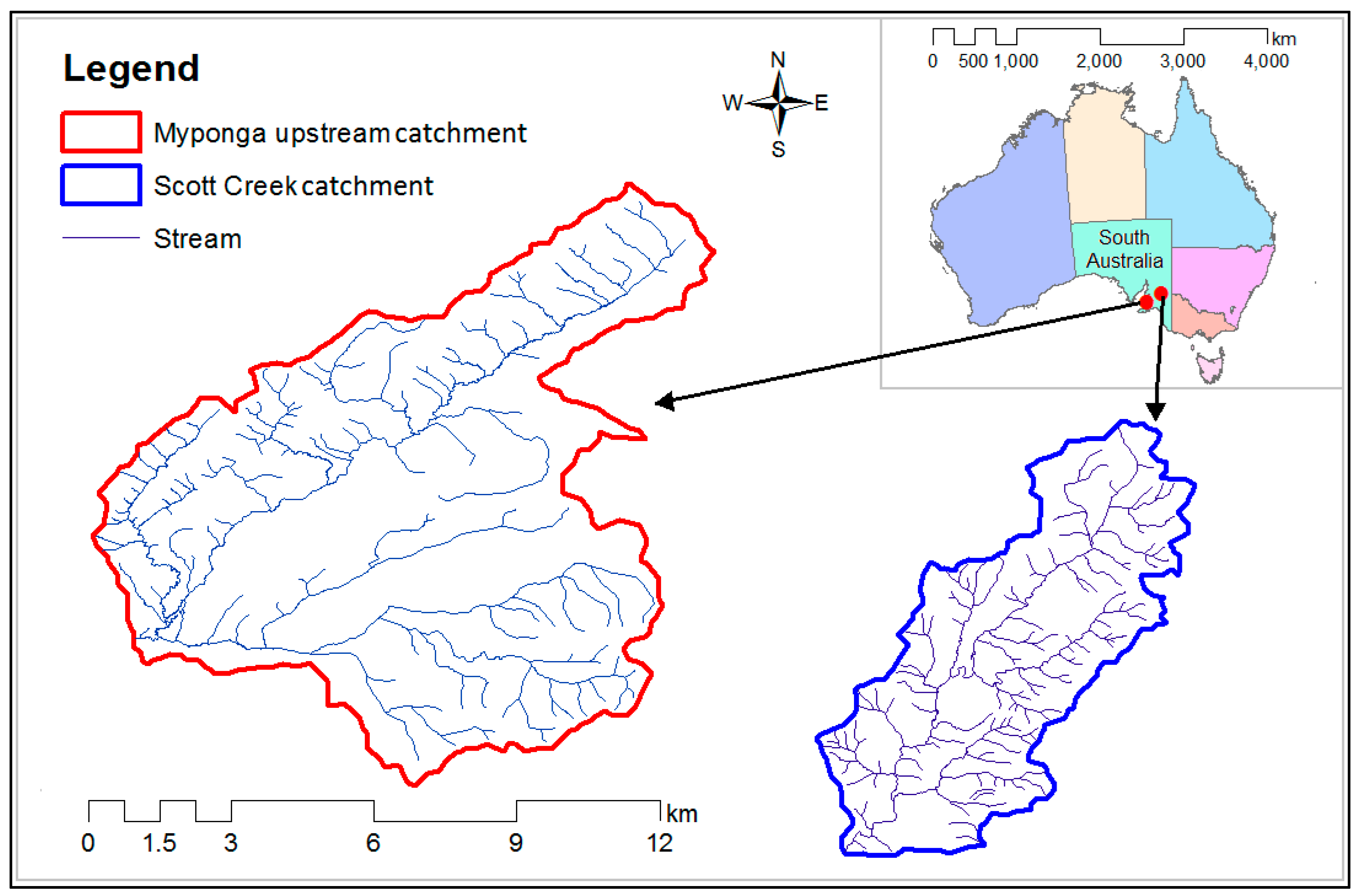
Scott Creek is a subcatchment of the Onkaparinga catchment located about 17 km southeast of Adelaide. The catchment spreads over an area of 26.6 km2. The runoff from Scott Creek is highly seasonal, being concentrated in the winter and spring seasons. The mean annual streamflow measured at the Scott Bottom gauging station, is 3,710,000 m3/year (MDF = 0.12 m3/s) [15]. The topography of the catchment varies from steep slopes to mild rolling terrain [52]. A range of soil categories exists in the catchment. The northern and eastern sides of the catchment comprise loamy sand soils while north western and southern parts are mostly characterised by loam. About 51% catchment land consist loamy sand, 31% loam and 15% sandy loam [15,50]. The aquifer in the region is characterised by fractured rock aquifers which are overlain by a thin soil layer [51]. Groundwater plays a vital role in streamflow generation from the Scott Creek catchment [58]. The climate of the catchment is typically temperate with cool moist winters and warm dry summers. The average daily temperatures ranging from 14 °C to 27 °C in summer and 8 °C to 14 °C in winter [57]. The mean annual rainfall and evaporation in the catchment is 992 mm/year and 1200 mm/year respectively [57]. A location map of the Myponga upstream and Scott Creek catchment is shown in Figure 1.
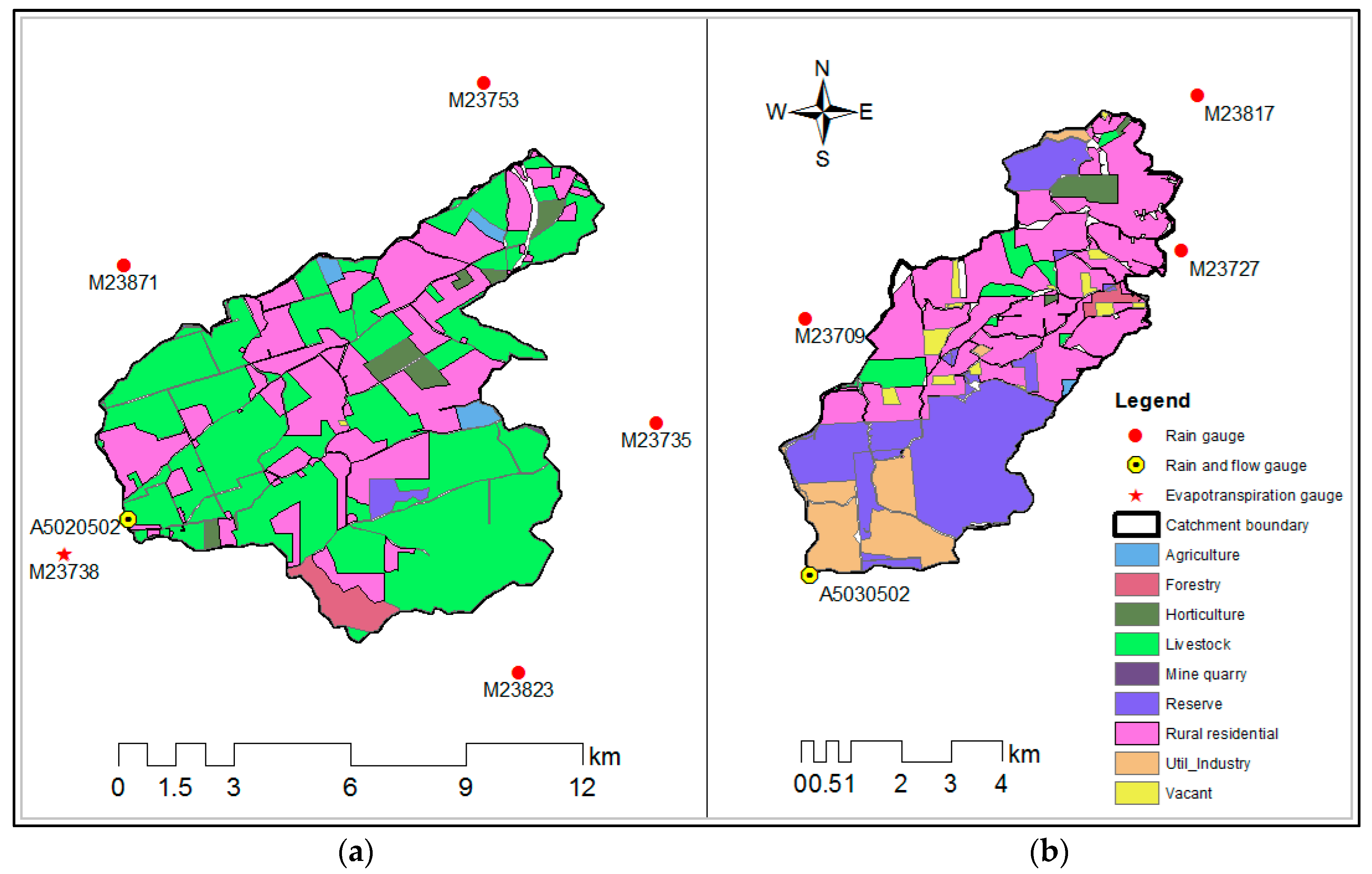
Land-use distributions for Myponga upstream and Scott Creek catchment are shown in Figure 2a,b. As can be seen in Figure 2, majority of the land at the Myponga upstream covers by livestock which includes broad scale grazing for cattle and sheep. According to Wella-Hewage [15], approximately 75% of the catchment area is used for grazing, 16% covered by native vegetation, 7% covered by native forest and 2.4% used for horticulture. On the other hand, grazing is the major land-use of Scott Creek catchment, covering almost 50% of the catchment area, while natural vegetation covers 48% of catchment area. Natural vegetation exists mostly on the steep slopes of the catchment. The remaining land-uses includes 0.5% plantation forest and 0.8% urban areas [15].
2.2. EPA-SWMM Model Description
The EPA-SWMM model was first developed in 1971 (SWMM1) and since then it has undergone four major upgrades: SWMM2; SWMM3; SWMM4; and SWMM5. The current version (SWMM5) has many attractive features including an integrated graphical environment to do the modelling task in a more convenient way. It also offers several post-analysis options such as displaying simulation result using graphs and tables, showing drainage area maps, scatter plots, profile plots, etc. Under version 5, the model has several releases. This study used release 5.1.011 to perform the analysis.
EPA-SWMM is a conceptual RR model that can be used for urban and rural, EB as well as CS modelling. The model is capable of accounting spatial variability of catchment properties by dividing the catchment into a collection of smaller, homogeneous subcatchments. It consists of four groups of algorithms to describe the hydrological processes of a catchment. These are: (i) surface runoff algorithms; (ii) loss algorithms; (iii) conveyance algorithms; and (iv) groundwater flow algorithms [11,40,41]. Surface runoff algorithms are used to generate surface runoff hydrographs from subcatchments. The model uses nonlinear reservoir routing techniques to compute surface runoff from each subcatchment [40]. Loss algorithms are used to estimate stormwater losses in a subcatchment due to infiltration and evaporation. Evaporation/evapotranspiration losses are modelled as losses from three different levels. These are: (i) surface; (ii) unsaturated zone; and (iii) saturated zone [11,40]. Infiltration losses are calculated using one of the three methods, viz. Horton method, Green–Ampt method or the Soil Conservation Service (SCS) Curve Number method [41]. The Horton method assumes infiltration rate to be maximum at the beginning of a storm and is decreasing exponentially with time and reach to a minimum constant or equilibrium rate when the soil gets fully saturated [11,40]. The Green–Ampt method describes the infiltration process as a balance between the changing water content of the soil over time and the change in hydraulic conductivity and diffusivity through the depth of the soil profile. The SCS curve number method is an empirical method based on the classification of several parameters describing the direct runoff and soil types for different areas across the United States. This method considers the runoff as a function of the total precipitation, the potential maximum storage retention and the initial abstraction.
The subsurface flow algorithms controls infiltration of water to the aquifer and groundwater flow [11,40,41]. Aquifers are represented in the model by two zones: unsaturated or upper zone and saturated or lower zone [40,42]. The upper zone receives water from the subcatchment through infiltration. The flow from the unsaturated zone to the saturated zone is controlled via infiltration parameters which depend on the moisture content of the upper zone. Water in the saturated zone is routed as lateral inflow to the stream and percolation into deep groundwater. Conveyance algorithms are used to route water through a conduit link. Flow within a conduit link is routed using one of the three routing methods, viz. steady flow routing, kinematic wave routing or dynamic wave routing [41,43]. Steady flow routing assumes flow is uniform and steady within each computational time step and hence does not account for channel storage, backwater effect, entrance/exit losses etc. Kinematic wave routing assumes energy slope equals the bed slope and each conduit is able to accommodate flows up to a maximum flow level and the excess water is stored in the upstream node and routed when capacity is available. Dynamic wave routing uses the one-dimensional Saint-Venant flow equation, coupled with a one-dimensional continuity equation and full momentum equation. This method is capable of accounting channel storage, backwater effects and entrance/exit losses [11,15,40,41,42,43]. The continuity equation is applied at each node of the conveyance system while the momentum equation is applied along the conduit links.
2.3. Data
Rainfall–runoff modelling with EPA-SWMM requires rainfall and evaporation data as input to the model. There are several gauging stations in and around the Myponga upstream and Scott Creek catchments those are managed by the Bureau of Meteorology (BOM) and Department for Environment and Water (DEW). Some of these gauging stations record data on daily time-scale while others on sub-daily scale. Available data for these gauging stations were collected from BOM and DEW. These data were assessed for quality and only a few gauges were found to have continuous record on daily scale and selected for the modelling tasks. The selected gauging stations for both catchments are shown in Figure 2. Other data, including SRTM (shuttle radar topographic mission) derived one-arc-second (~30m) gridded digital elevation model (DEM) data, geological cross-section data of the catchments, soil category data and land-use data were collected from the Geoscience Australia and South Australian Government’s Spatial and Geographic Information System (GIS) databases.
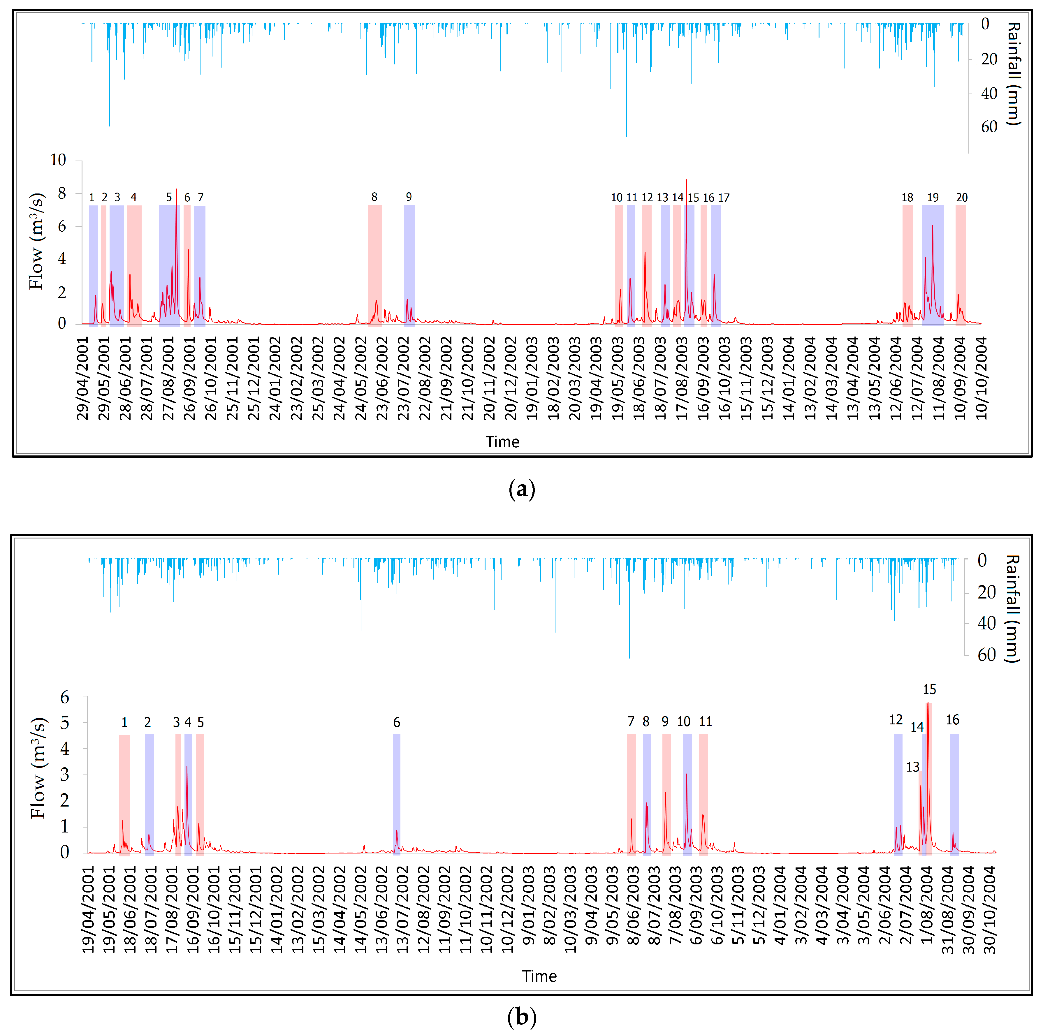
Though the collected time series data of the selected gauging stations spans over several years, the complete series could not be used because of: (i) missing records; and (ii) data from all selected gauges’ do not coincide with each other for several reasons including shifting gauges and instrument malfunction. Finally, records from year 2000 to 2007 was found to be the longest continuous record which was graded as good quality by the agency and therefore selected for the study. These time series data were divided into three parts; the year 2000 was allocated to be the continuous RR modelling warm up period [15,59], while the periods from 2001 to 2004 and from 2005 to 2007 were chosen to be the model calibration and validation periods respectively in the EPA-SWMM modelling. The ratio of 70:30 was applied in allocating data series for model calibration and validation periods. A warm-up period is allocated for a continuous RR model before the actual calibration is performed to enable the model parameters to adjust to the current hydrological conditions. This period may less for wet catchments (ratio of evaporation over precipitation <0.90) and high for dry catchments [59]. According to Rahman et al. [59], a wet catchment requires less time (~55 days) as warm up in comparison to that of dry catchment (~298 days). From the calibration period (2001–2004), events that produce peak flow above a threshold value, which was fivefold higher than the mean annual flow were extracted for the EB model calibration. As the peak flow of the selected events are with Annual Exceedance Probability (AEP) greater than 0.5, these events are considered as more frequent events in the context of flood frequency studies. Finally, a total of 20 streamflow events at the Myponga upstream catchment and 16 at Scott Creek catchment were selected, as indicated in Figure 3a,b. The selected events covered a wide range of peak flow levels ranging from 1.2 m3/s to 8.8 m3/s at the Myponga upstream and 0.7 m3/s to 5.7 m3/s at Scott Creek catchment.
Even though the collected time series data was graded as good quality by the agency, they were further checked for errors. Bonnin et al. [60] suggested that for good quality data checks, it is important to ensure: (i) check for extreme values above threshold; (ii) a real-data-check of values among others; (iii) dataset trend analysis; and (iv) a study of cross correlation between the gauges. Data were checked for outliers, normality and homogeneity by using parametric and nonparametric tests [61,62]. Outliers were defined by values over M + 3SD (M is the mean and SD is standard deviation) and compared with values from other gauging stations. If similar record exists in other gauging stations, they were not treated as outliers otherwise replaced by either mean value or M + 3SD as appropriate compared to the other gauging stations. Kolmogorov–Smirnov and Shapiro–Wilk’s test of normality was done on the datasets and found that none of these gauges’ data were normally distributed. However, the standard normal homogeneity test (SNHT) indicated that there was no significant difference between variances of different rain gauge’s data for both catchments at 0.05% significance level. Besides, correlation analysis indicated that significant correlation exists within all rain gauges’ data at both catchments. As shown in Figure 4a,b, trend analysis suggests that despite the fluctuations in annual rainfall and annual streamflow, a general trend of decrease in rainfall was consistent with the trend of decrease in streamflow at both catchments.
2.4. Catchment Delineation and Model Setup
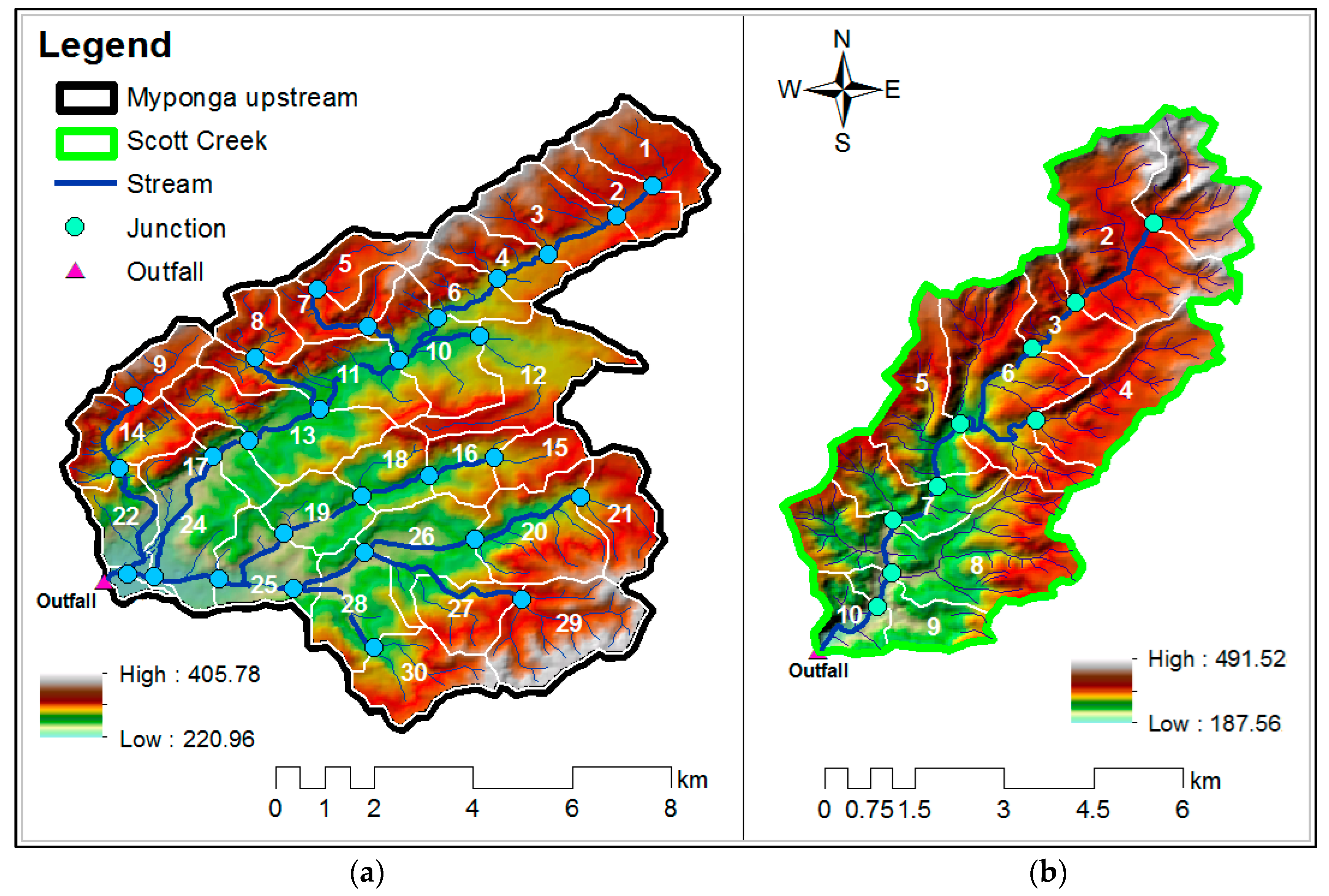
Catchment processes are highly variable at both spatial and temporal scales [63]. To account for spatial variability, the Myponga upstream and Scott Creek catchments were subdivided into thirty and ten subcatchments, respectively, by using ArcMap software and 1-arc-second DEM data. Spatial analyst tools in ArcMap offers a range of functions to perform the catchment delineation. First a depressionless DEM layer is created to avoid any internal drainage within the catchment. This layer is then used to create flow direction and flow accumulation layers in ArcMap where it shows flow accumulations in streams, classify these streams based on flow accumulations and displays the classification with the help of color ramp. On the streams, several pour points to be identified where significant variation in flow accumulation occurs, roughly indicating on how many subcatchments to be created. There are no specific rules on the number of subcatchments required for modelling but the RORB model manual suggests that between 5 and 20 subcatchments are enough to allow for spatial variation of terrain, rainfall and losses [12]. Hence, by interpreting the flow accumulation layer in ArcMap, it was apparent that thirty subcatchments for Myponga upstream and ten for Scott Creek catchment were reasonable and pour points were inserted accordingly. The flow direction layer, flow accumulation layer and pour points layer were then processed through a few more functions in ArcMap and finally created the delineated watershed. In the EPA-SWMM model, water from every part of a subcatchment is flowing towards a common node and from that node, it is then routed to the next node through a conduit link between the nodes. Figure 5a,b presents the delineated subcatchments and main flow paths for the Myponga upstream and Scott Creek catchments.
After the subcatchment delineation, some model parameters such as width and slope of a subcatchment, conduit length and junction invert elevation were extracted using GIS and DEM data. Percentage of impervious and pervious areas were estimated by interpreting the land-use map. Manning’s roughness for impervious and pervious areas for each subcatchment was assigned via estimation using aerial photographs of the catchment. The initial values of depression storage parameters were assigned within the values recommended in the EPA-SWMM manual for various land-use types [40,41]. Though EPA-SWMM model allows to model irregular channel cross-sections, field observations suggested that stream cross-sections of the Myponga upstream and Scott Creek catchments can be simplified into trapezoidal geometry. Therefore, conduit sizing was estimated by assuming trapezoidal cross-section and depth of conduit was estimated as 3 m. Besides, some previous studies at the Myponga upstream and Scott Creek used trapezoidal cross-section in model setup and obtained a reasonable modelling performance [15,17]. Conduit roughness was initially assigned a value of 0.10 as per the recommended values in the EPA-SWMM manual [41,42]. The EPA-SWMM manual suggests that the depth of junction invert should be at or below the channel invert [40,42]. Hence, the depth of junction invert was assigned an arbitrary value of 4 m to keep it below the channel invert of 3 m. For infiltration modelling, the Horton infiltration method was selected because of its superiority over other infiltration methods such as Green–Ampt method, or SCS curve number method. Horton’s method is widely adopted in infiltration modelling as it can best represent the infiltration capacity curve [15,64]. The initial values of the Horton’s infiltration parameters were assigned by interpreting the hydrological soil group map and using the recommended values provided by Akan [18].
Aquifer bottom elevation was obtained from the geological cross-section map of the catchments. Initial aquifer water table depths for each subcatchment was estimated as equal to the junction invert elevation. Other aquifer properties such as field capacity, wilting point, and hydraulic conductivity for the identified soil categories in the catchments were obtained from the EPA-SWMM manual [40,41]. The initial soil moisture content in the aquifer was assigned an arbitrary value between the field capacity and the wilting point of the subsoil. Conductivity slope and seepage were assigned arbitrary values within the range specified in the EPA-SWMM manual [40,42]. Tension slope was initially assigned as EPA-SWMM default value and the initial value of the upper evaporation fraction was assigned an arbitrary value. The elevation of the ground surface level was set at a level 4 m higher than the node invert elevation. As the groundwater flow equation in the EPA-SWMM model is a user defined power function [11,41], initial values of the groundwater flow coefficient and exponent were assigned default values.
As shown in Figure 2, rainfall data were available from five rain gauges at the Myponga upstream and four gauges at the Scott Creek catchment. In order to identify which station’s rainfall data is most relevant to a given subcatchment, the contributing area for each gauging station was determined using the Thiessen-polygon method. This method is widely used not only in Australian context but also around the world. Some of the previous studies at the Myponga upstream and Scott Creek catchment were done using this method [15,17]. Consequently, subcatchments within a gauging station’s Thiessen-polygon boundary were assigned rainfall from that gauging station. Unlike rain gauge stations, evaporation gauges are sparsely located and therefore all subcatchments were assigned evaporation data from the closest evaporation gauge station.
The EPA-SWMM model was set up at daily time step because no suitable sub-daily time series data was available during the study period. For the flow routing option, the dynamic wave routing method was selected as it is theoretically the most accurate routing method, capable to simulate non-uniform, unsteady flow conditions. The routing time step in EPA-SWMM was set to 60 s. Although routing time steps with lower resolution (e.g., 30 s) can provide comparatively more reliable results, it requires a longer model run time and hence not preferable for automatic calibration where model needs to run several times during parameter optimization. The EPA-SWMM model allows to assign different time step values to compute surface runoff for different seasons of the year based on initial hydrological catchment conditions. Therefore, for dry periods, a time step of 10 min and for wet periods, a time step of 5 min were assigned to compute surface runoff. As year 2000 was considered as warmup period [59] for CS modelling, no events were selected from that year for EB modelling
2.5. Model Calibration, Validation, Parameter Sensitivity and Goodness-Of-Fit Tests
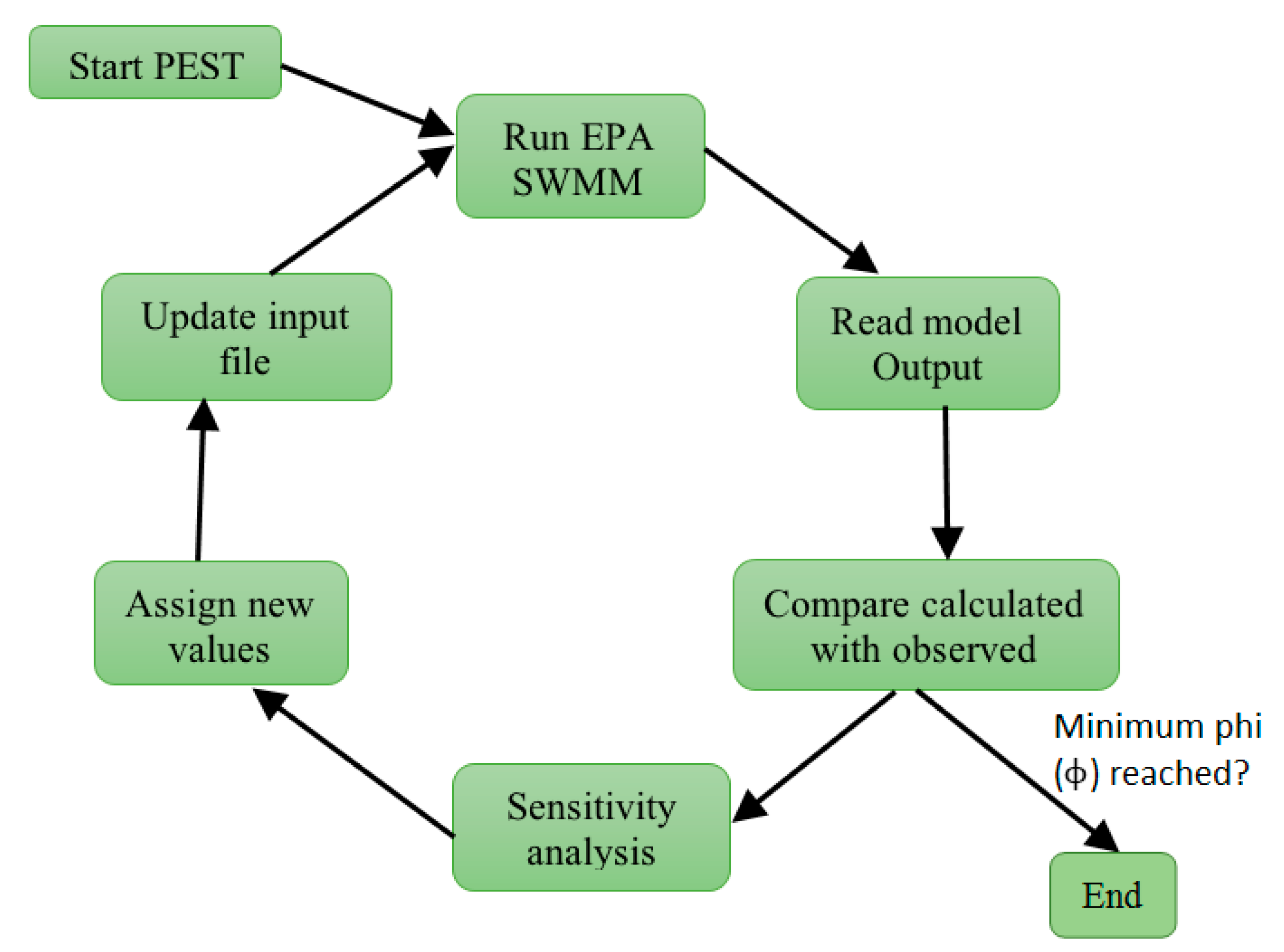
Both EB and CS models were calibrated using the automatic calibration method. A nonlinear parameter optimization tool, PEST (Parameter ESTimation) was integrated into EPA-SWMM to perform the optimization. In starting the process, PEST necessitates setting up three files: (i) PEST instruction file; (ii) PEST template file; and (iii) PEST control file [65]. The instruction file tells PEST how to read result from the EPA-SWMM modelling output file. For each model run during the optimization process, the PEST engine writes new values of the selected calibration parameters to the EPA-SWMM model input file using a template file. The PEST control file contains calibration data, initial values and upper and lower boundaries of the calibration parameters.
As shown in Figure 6, during the automatic calibration process, the PEST engine takes control of the EPA-SWMM model and performs a number of model runs within the assigned parameters boundary until a termination criterion is reached and the optimized values are identified. The termination criteria used in PEST are: (i) convergence of adjustable parameters to their optimal values (parameter convergence); (ii) insignificant relative parameter change over the successive iterations (function convergence); (iii) insignificant objective function reduction over successive iterations; and (iv) exceedance of the upper limit of the number of optimization iterations. The objective function used in PEST is given by Equation (1) [65].
where B is a vector comprising the parameters value being estimated, n refers to the number of total observations, and are the observed and simulated flow ordinates in ith observation and is the weight of ith observation.
Though several parameters were defined in the EPA-SWMM modelling, all of them do not need to be calibrated because some of them are insensitive as compared to the others and changing their values during optimization do not make any significant difference in the model output [15,40,65]. Therefore, the most appropriate set of parameters to calibrate was identified based on parameters sensitivity. Parameters that were extracted from GIS or taken from other available information were locked in the model and excluded from calibration. During the optimization process, at each model run, PEST slightly changes the parameter values from the previous run and observe its effect on the objective function. By comparing the objective function between two successive iterations, it computes parameters sensitivity which is recorded in the PEST sensitivity file. The calibration parameters sensitivities were investigated using the PEST sensitivity file and most sensitive parameters were identified within the first couple of runs. Finally, the calibration was carried out using these sensitive parameters while insensitive parameters were fixed at physically-sensible values. The parameters those identified as the most sensitive parameters during the sensitivity analysis are shown in Table 1. It was noticed from the sensitivity analysis in PEST that the most sensitive parameters are same in both CS and EB modelling but the level of sensitivity was different.
To assess the validity of the calibrated model, a model validation process was followed. CS model was validated within the period from 2005 to 2007. During the validation process, the model was run using rainfall and evaporation data for that period without changing the values of the model parameters obtained through the model calibration. In contrast, for the EB model validation, average model parameter which were calculated using the values of the calibrated events (20 events for Myponga catchment and 16 events for Scott Creek catchment) were adopted. Since the events used in the EB model calibration were from the wet part of the year, validation events were purposely selected from the wet period. Therefore, it was expected that by averaging the parameters would generally reflect the initial catchment conditions and the validation would be reasonable.
The performances of CS and EB modelling were evaluated by applying a total of 8 goodness-of-fit tests listed in Table 2. Among these goodness-of-fit tests, the Nash–Sutcliffe Efficiency (NSE) is widely used in comparable hydrological studies [9,15,17,47,66,67,68,69]. However, according to Jain and Sudheer [67], single values of NSE estimated using full series can be higher for poor models or lower for good models. In order to overcome this problem, NSE was calculated separately for wet seasons (ANSE) as well as for dry seasons (NSE of low flows), in addition NSE for the full series [15,66,70]. Moreover, Gupta et al. [71] reported that NSE is highly sensitive to large runoff volume and may not be linearly linked with model performance. To rectify this issue, they introduced a new goodness-of-fit measure called Kling-Gupta efficiency (KGE) that define the modelling performance in terms of three statistical components: the linear correlation, the bias and the variability of flow. This method has been widely adopted in recent studies including Saber and Yilmaz [69], Massari et al. [70], Kling et al. [72], Camici et al. [73], Dick et al. [74], Thirel et al. [75], etc. In addition to NSE and KGE, coefficient of determination (R2) [17,66,69,76], RSR which is defined as the ratio of root mean square error (RMSE) to the standard deviation of the observed series [77,78,79], absolute volume error [15,47,80,81] and absolute error in peak flow rate [47,80] were also used to assess the modelling performance.
Using these goodness-of-fit measures, the performance of both models was evaluated under two different scenarios: (i) performance in reproducing the observed streamflow hydrograph (total runoff hydrograph, TRH); and (ii) performance in reproducing the direct runoff hydrograph, DRH. In the first scenario, model performance was evaluated during the calibration period since the calibration was done to match with the observed streamflow hydrograph. To assess the models’ performance under the second scenario, baseflow was removed from the observed and the simulated time series before the goodness-of-fit tests were conducted. A variety of baseflow separation techniques are available in the literature [29,30,31,32,33]. The common separation method to calculate the baseflow from the time series records can be performed either by: graphically or by filtering. The graphical methods are generally employed to plot the baseflow component of the flood hydrograph [31,33]. They attempt to identify points on the hydrograph where baseflow intersect the rising and falling limbs of the quick response. In this way, they delimit the entire baseflow hydrograph. Among these graphical methods, it is possible to highlight three approaches: the constant discharge; the constant slope method; and concave method [32]. The filtering separation methods on the other hand use data filtering procedure to separate the baseflow component of streamflow time series [29,30]. They are designed to generate a baseflow hydrograph for a long-term period of observations. The aim of this approach is the generation of an objective, repeatable and easily automated index known as the baseflow index, which is a long-term ratio of baseflow to total streamflow. This study utilized a baseflow separation tool, “BFI+” [31] that uses graphical local minimum method proposed by Sloto and Crouse [33]. The local minimum method searches the minimum flow record within a time interval and assume it as the baseflow component. The interval is defined as days before the day being considered to days after the day being considered, where ; A being the watershed area in square miles [28]. This point is then connected by straight lines to adjacent local minima. The baseflow for each day between these points is estimated by linear interpolation. This method is illustrated in Figure 7.
Finally, to assess the overall modelling performance, a statistical framework for interpreting hydrological model performance developed by Ritter and Muñoz-Carpena [76] was adopted. Similar classification can be found in the literature [47,68,77] that assesses the goodness-of-fit into four different performance classes as shown in Table 3.
3. Results
3.1. Parameter Sensitivity
During the optimization process, it was observed that for CS modelling, groundwater parameters, unsaturated zone moisture content, channel roughness and seepage were the most sensitive parameters, while depression storage and Manning’s roughness for pervious area were comparatively less sensitive. For EB modelling, unsaturated zone moisture content and channel roughness showed high sensitivity, while surface runoff parameters and groundwater parameters showed comparatively less sensitivity. The sensitivity analysis in PEST suggested that for CS modelling, optimization is mainly governed by the groundwater parameters, unsaturated zone moisture content, channel roughness and seepage characteristics, whereas for EB modelling, the optimization process is mainly driven by the unsaturated zone moisture content and channel roughness.
3.2. Model Performance during Calibration and Validation
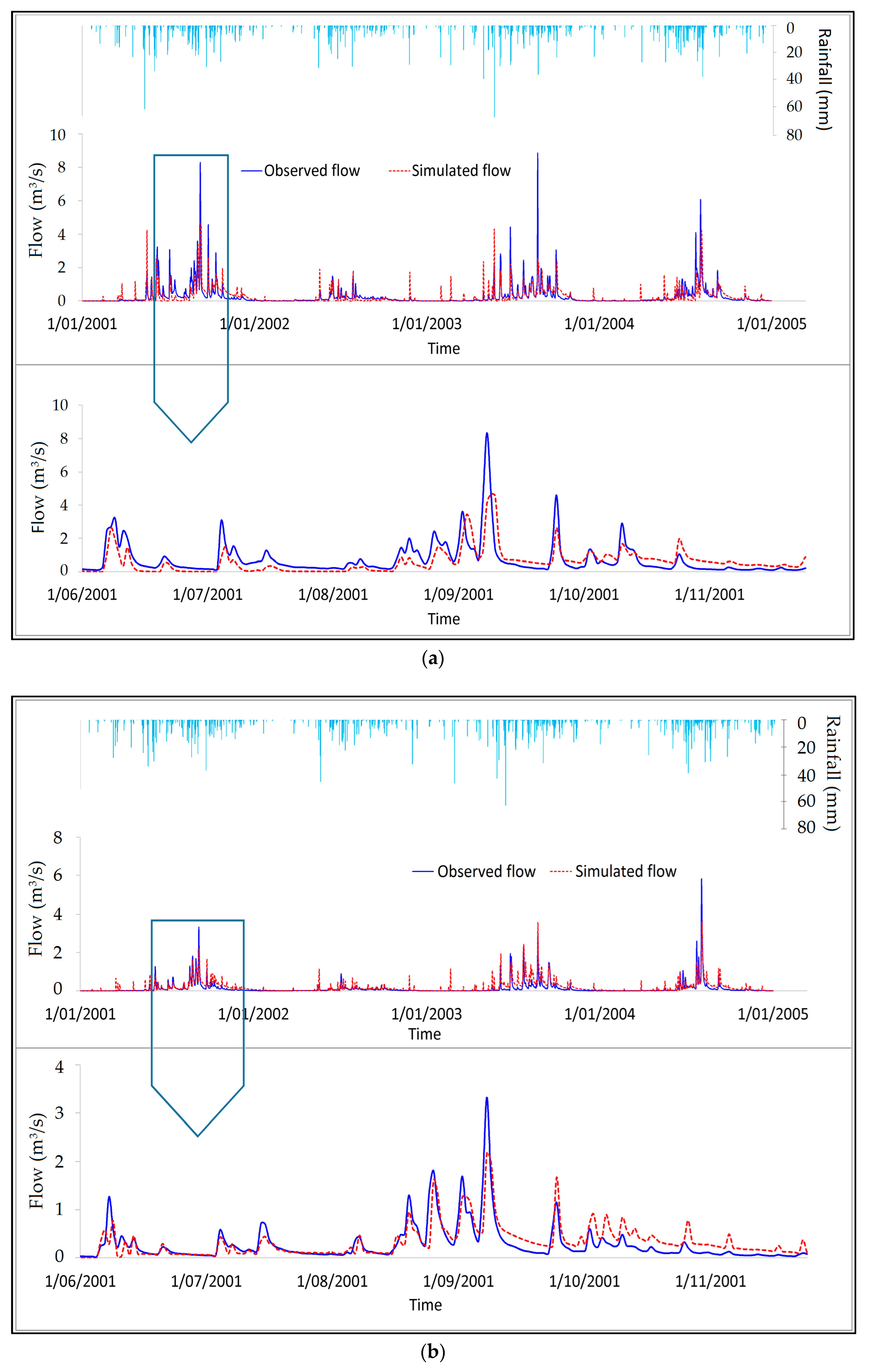
After the model optimization was completed, the EPA-SWMM model was then run with the optimized parameters. Figure 8a,b compare the observed and the simulated (CS modelling) time series against the rainfall time series at the two study catchments. Visual comparison indicates that the trend in the simulated series resembles the observed series reasonably well. However, it is apparent that, simulations of the extreme events were not highly successful.
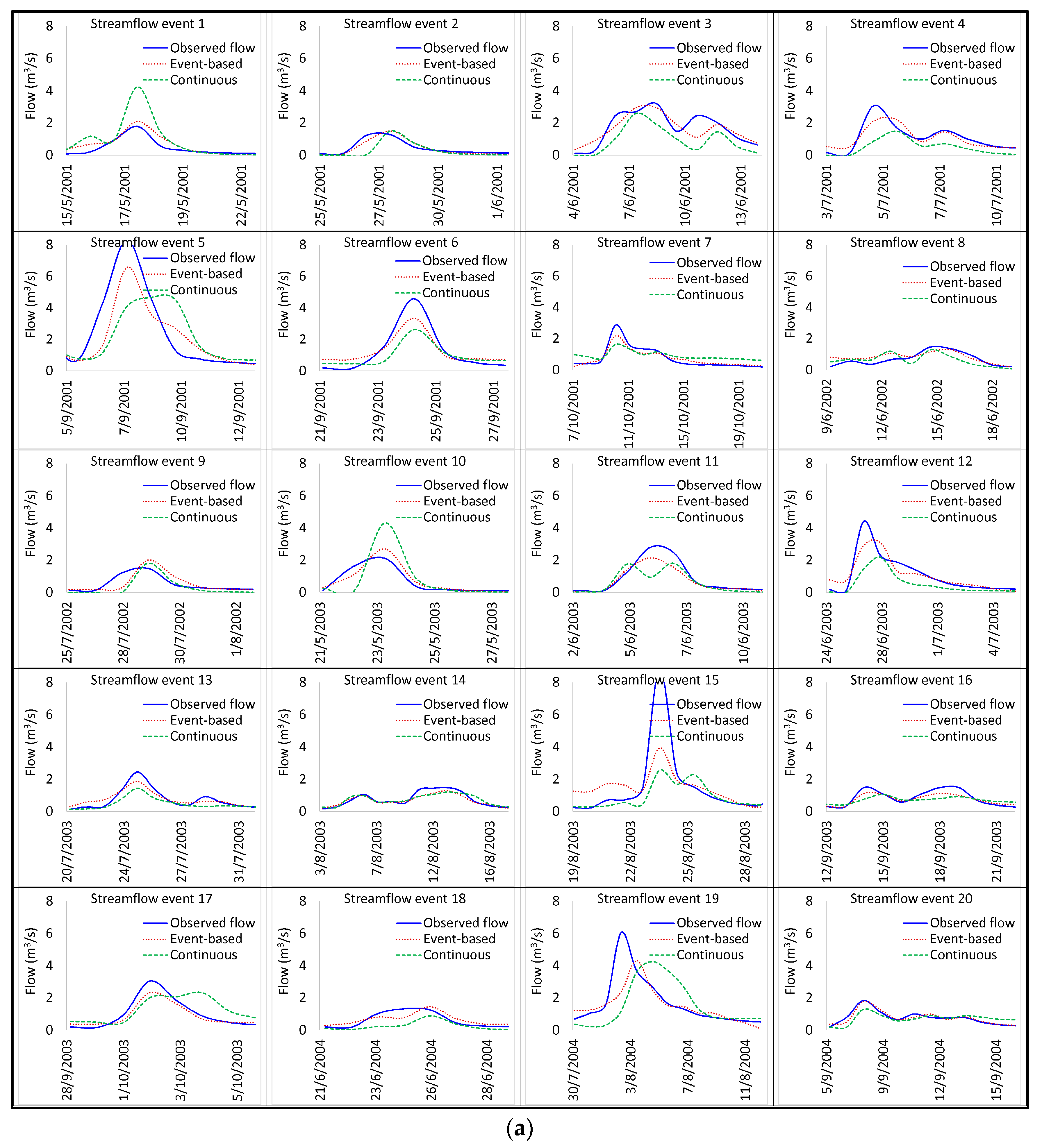
The EB model was calibrated individually for the selected events at two case study catchments. Figure 9a,b compare the simulated hydrographs by the EB model and the CS method against the observed hydrographs at the Myponga upstream and Scott Creek catchments respectively while the goodness-of-fit values for these events are presented in Table A1, Table A2, Table A3 and Table A4 in Appendix A. It is apparent that, for most of the events, the simulated hydrographs by the EB model resemble the observed hydrographs more closely. Also note that simulated hydrographs for Events 1 and 8 by the two models for Scott Creek are matching each other but not reflecting the observed hydrograph. This could be due to errors in the observed rainfall data. This issue was further evident through the values of the performance indices given in Table A3 and Table A4 in Appendix A. Therefore, in calculating average results, (e.g., Table 4), these two events will be excluded.
Performance of the EB and CS modelling are compared here using the goodness-of-fit measures listed in Table 2 and the assessment framework shown in Table 3. As noted in Table 2, when the scores for either NSE (NSE, ANSE and NSE for low flows) or KGE or R2 is higher than that of the other model type, it is said to be outperforming. The opposite will apply with RSR, absolute volume error and error in peak flow criteria. At the Myponga upstream catchment, the average scores of the NSE for full period (NSE), NSE for wet season (ANSE), NSE for low flow season and KGE were estimated as 0.50, 0.56, −0.015 and 0.68, respectively. This indicates that, overall, the model is capable of simulating daily flow series or daily high flow series with a reasonable level of accuracy but incapable of simulating low flow series. Based on the framework of statistical interpretation developed by Ritter and Muñoz-Carpea [76] and Singh et al. [77], the performance level of the CS model calibration can be regarded as “satisfactory”. On the other hand, in EB modelling, the average scores of NSE, ANSE, NSE of low flows and KGE were 0.75, 0.76, 0.65 and 0.73 respectively, indicating that the performance level was “good”.
In terms of coefficient of determination (R2), EB model (R2 = 0.82) outperformed the CS model (R2 = 0.51). RSR value, that is determined by dividing RMSE by the standard deviation of the observed flow series was 0.46 for event based-modelling and 0.64 for CS modelling, which further confirms that EB model performs better than the CS model at the Myponga upstream catchment. Mean daily flow of the observed and the simulated series by CS modelling during the calibration period were 0.27 m3/s and 0.25 m3/s, respectively, with an overall 9% of absolute volume error. EB modelling shows slightly better performance in simulating observed hydrograph by having only an 8% of absolute volume error. Average percentage error in peak flow rate of 22% and 48% also indicate that EB modelling is better than CS modelling in achieving peak flow objective. Overall, the performance of the EB modelling can be accepted as “good” category and it outperforms the CS modelling at the Myponga upstream.
CS modelling at Scott Creek catchment, achieved goodness-of-fit scores of 0.54, 0.71, 0.68 and 0.38 for NSE, ANSE, NSE of low flows, and KGE respectively. A comparatively high value of ANSE indicates that the model has a high capability of simulating high flows. Based on NSE and ANSE, model performance is at “satisfactory” level (NSE, ANSE > 0.50) although KGE value does not fall within the same category. Performance of the EB model was also found to be at “satisfactory” level by having scores of 0.56, 0.57, 0.51 and 0.63 for NSE, ANSE, NSE of low flows and KGE respectively. The R2 was 0.75 which also ensured a good agreement between the observed and the simulated flow than that achieved from CS modelling (R2 = 0.61). Absolute volume error and error in peak flow estimation in EB modelling were 17% and 25% with compared to 48% and 37% in CS modelling. Consequently, though the performance of both models were rated at “satisfactory” level, these measures confirm that the EB model outperformed the CS model at Scott Creek during the calibration period.
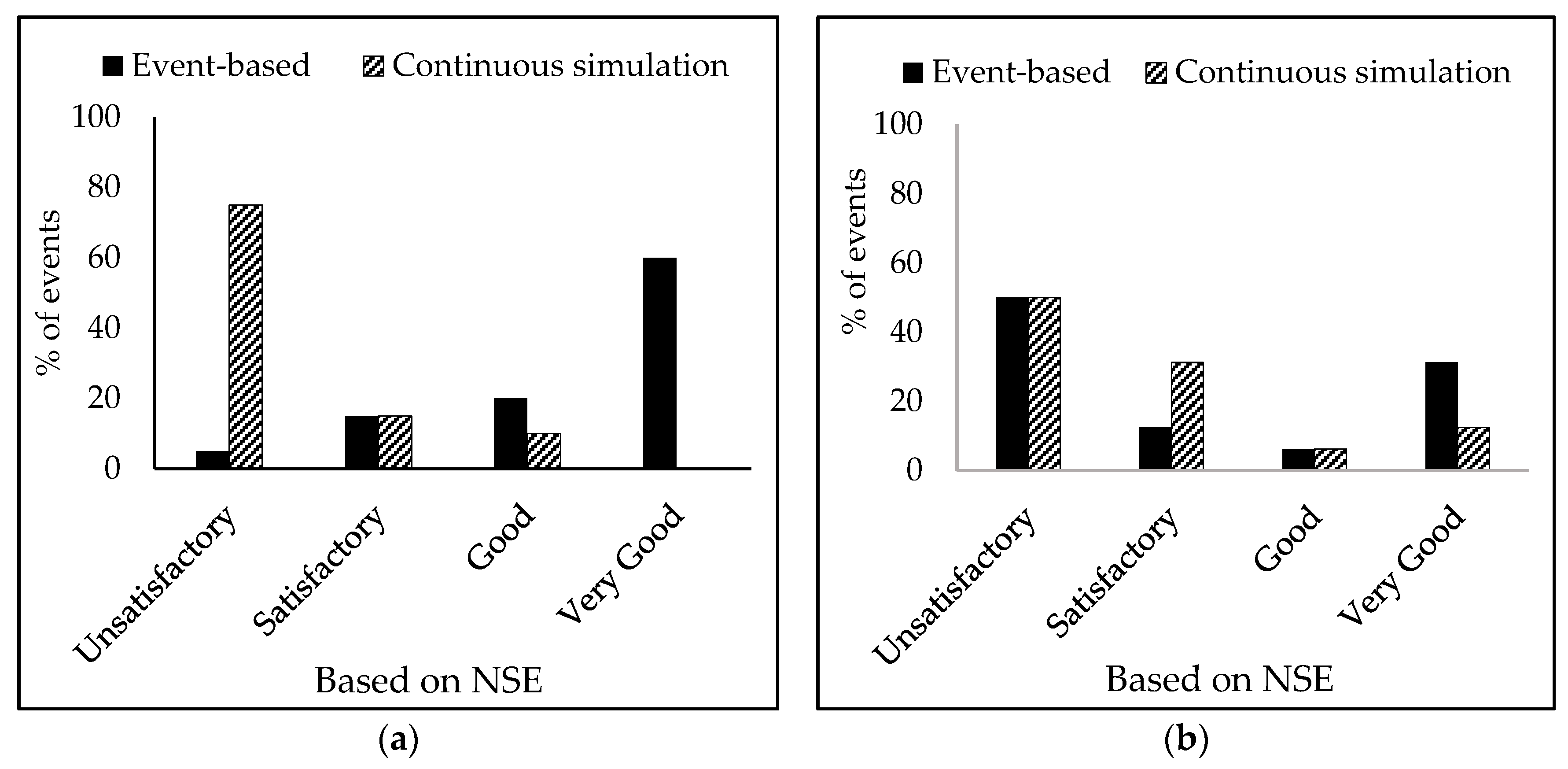
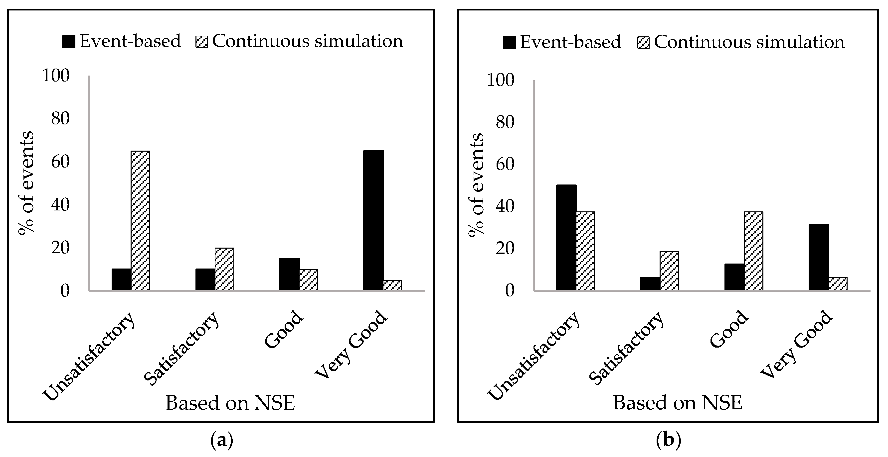
As the model goodness-of-fit scores vary from one event to another, recommending one grade (“satisfactory” or “good”) to a whole catchment based on an average score can be misleading. Hence, it was decided to examine the performance grade distribution over the events. For example, Figure 10a,b present NSE data for the Myponga upstream and Scott Creek respectively. It is clearly observed from Figure 10a, that while CS model was unsatisfactory for over 70% of the events, EB model was giving top level performance for over 60% of the events at the Myponga catchment. Also observed from Figure 10b, is that 50% of the time both models were not satisfactory while for the majority of the remaining events, EB model was outperforming (having “very good” grade for over 30% of the time) than CS model. These observations suggest that based on performance measured in terms of NSE, EB model outperform the CS model at both the case study catchments.
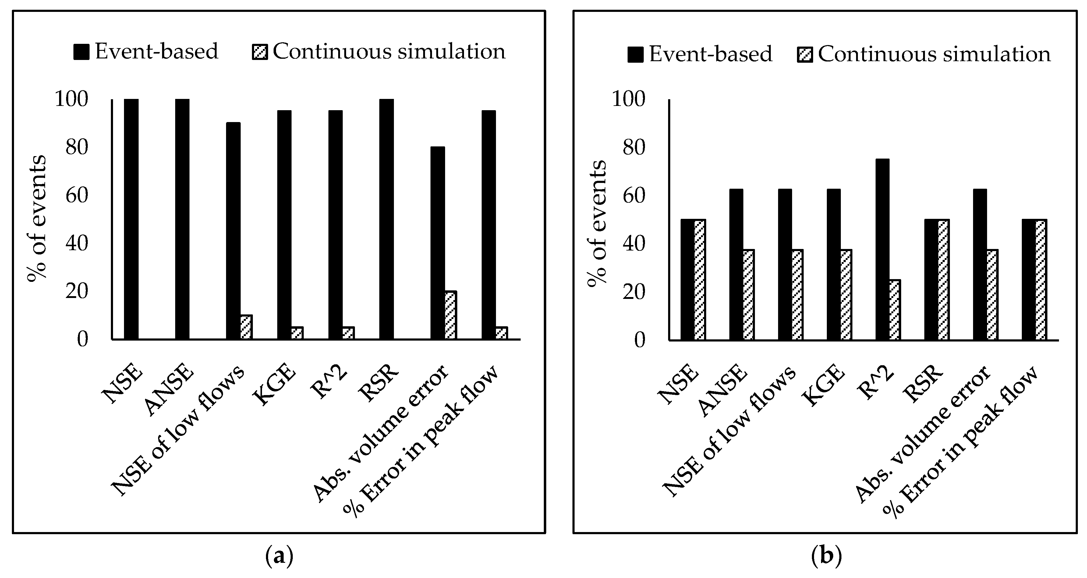
Figure 11 shows percentage of events that each model type outperformed the other in terms of any given goodness-of-fit measures.
Further, as observed in Figure 11a,b, the EB model outperformed the CS model in terms of all selected goodness-of-fit criteria at the Myponga upstream catchment and 6 out of 8 criteria at Scott Creek catchment. More importantly, it is noted that EB model was better performing at greater proportion of the events (95%) at the Myponga while it equally performed as CS model at Scott Creek in achieving peak flow target.
Outcome of the CS model during the validation period at the study catchments are presented in Figure 12a,b. It is observed from Figure 12 that the resemblance of the predicted flow to the observed flow is poorer than that was observed during the calibration period (Figure 8) at both the catchments.
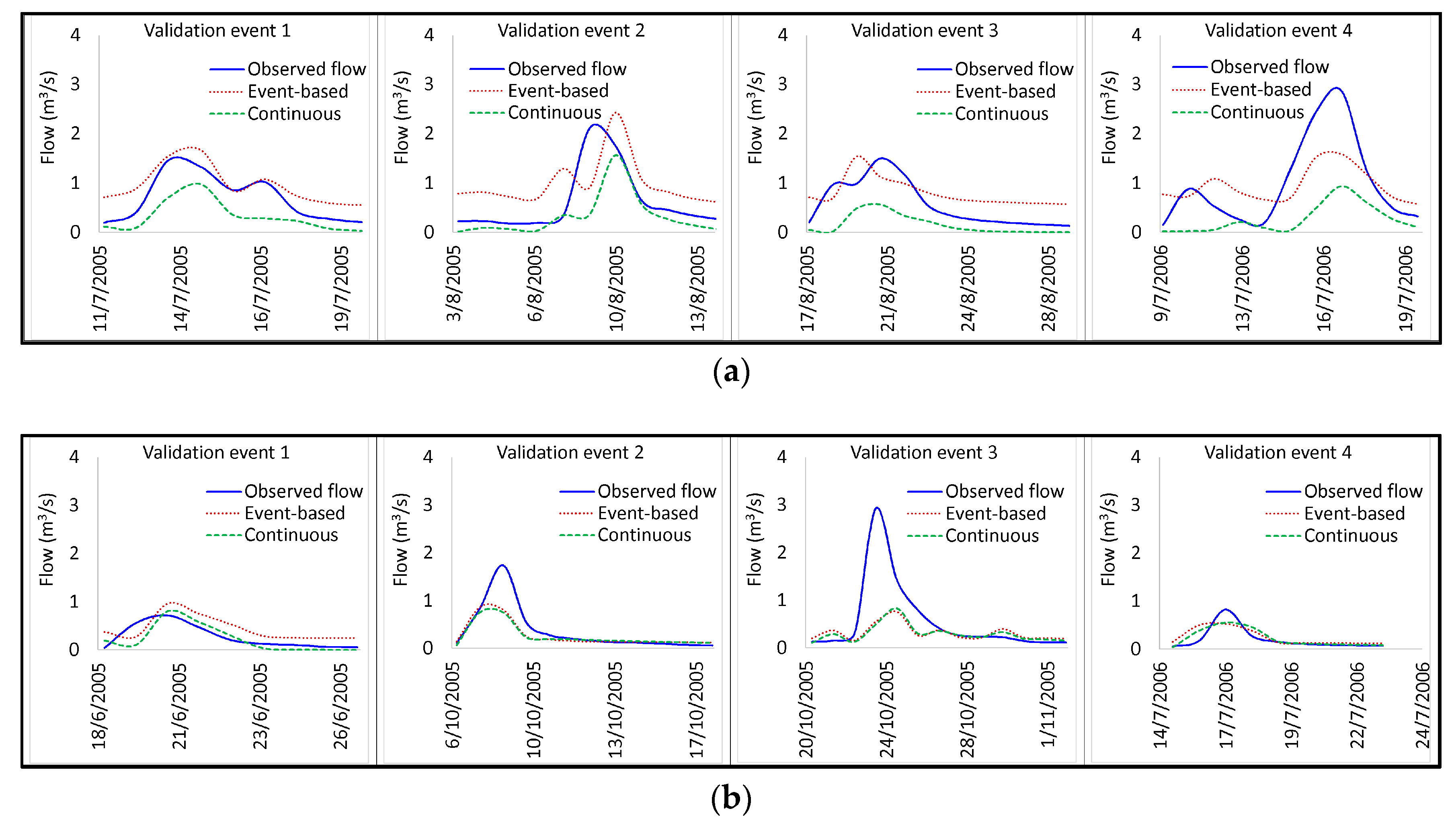
As noted earlier, EB model validation was done by using the mean parameter values. Four streamflow events were extracted from the validation period to evaluate the validity of the calibrated model. Three out of four extracted events were from the year 2005 because year 2006 was comparatively dry and only one event with a reasonable peak was available for model validation. Figure 13a,b present how the simulated hydrographs by the two methods compare against the observed hydrographs at the Myponga upstream and Scott Creek catchments respectively. It is noted from Figure 13a that the simulated hydrographs by the EB model resemble the observed hydrographs more closely than that of the CS model. In contrast, at Scott Creek catchment, simulated hydrographs of both EB and CS models resemble each other well and follow the trend of the observed hydrographs but both models underestimate the peak flow and the flow volume in 3 out of the 4 events.
Table 5 presents average goodness-of-fit scores of the two models at the study catchments during the validation period. As can be seen from the Table 5, at the Myponga upstream catchment, average values of goodness-of-fit measures; NSE, ANSE, NSE of low flows and KGE for CS modelling were 0.40, 0.47, −0.54 and 0.39 respectively while respective values of the EB modelling were 0.32, 0.48, 0.10 and 0.29. Consequently, performance of the both models are at “unsatisfactory” level during the validation period. On the other hand, at Scott Creek catchment, based on average scores of NSE, ANSE and KGE, the performance of the EB model can be rated as “unsatisfactory” while that of the CS model can be accepted as “satisfactory”. The R2 and RSR values also support these claims. Absolute volume error resulting from the two models were reasonably high at the Myponga while CS model at Scott Creek was surprisingly achieving good volume balance (2% of absolute volume error).
Poor model performance during validation may be due to several reasons including poor data quality, overfitting the model during calibration and spatial and temporal variations in catchment characteristics between the calibration and validation periods. Further, the goodness-of-fit scores estimated during the validation period cannot be taken as reliable as the calculation was based on only 4 events. However, considering the observations made in Figure 12, a good agreement between the rainfall hyetograph and simulated flow hydrograph at both catchments suggests that, the validation of the CS model can be considered as acceptable.
3.3. Model Performance in Reproducing Direct Runoff Hydrograph (DRH)
As stated before, EB and CS modelling performances were assessed under two different scenarios: (i) the performance in reproducing TRHs; and (ii) the performance in reproducing DRHs. Results of the scenario 1, were presented in Figure 9. As observed in Figure 9 and discussed in Section 3.2, at both Myponga upstream and Scott Creek catchments, simulated total hydrographs of the EB modelling showed relatively better agreement with the observed hydrographs than that of the CS modelling. Further, EB model performance was rated as “good” at the Myponga upstream and “satisfactory” at Scott Creek based on average scores of goodness-of-fit measures; NSE, ANSE and KGE. On the other hand, CS modelling showed a lower performance, i.e., “satisfactory” at Scott Creek and “unsatisfactory” at the Myponga upstream catchment.
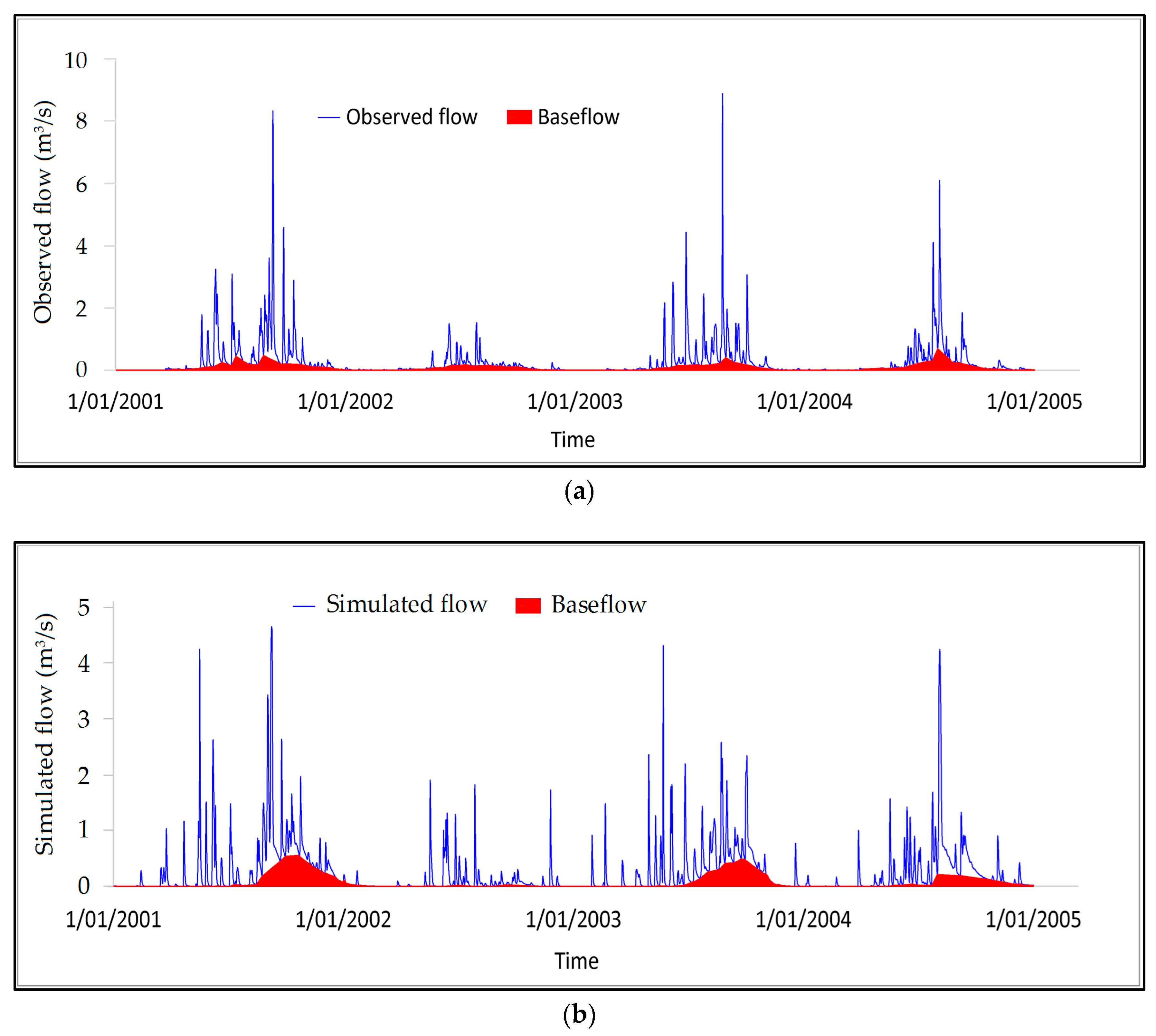
In the second scenario, that is performance in reproducing DRHs was assessed. To obtain DRH, baseflow was first separated from the observed and the simulated hydrographs following the procedure described in Section 2.5. The baseflow separation of the observed time series and CS modelling time series at the Myponga upstream are presented in Figure 14a,b. It is apparent from Figure 14 that baseflow component of the simulated time series is relatively higher than that of the observed time series. Therefore, it is vital to understand how two modelling methods perform in predicting DRHs.
Table 6 compares the average scores of the 8 selected goodness-of-fit criteria in reproducing DRHs by the two modelling methods at the two case study catchments. The individual scores of each event are presented in Appendix A, Table A5, Table A6, Table A7 and Table A8. The average scores of NSE, ANSE, NSE of low flows and KGE for EB modelling at the Myponga upstream were 0.75, 0.73, 0.86 and 0.74 respectively whereas respective scores for CS modelling were 0.26, 0.20, 0.55 and 0.45. These values clearly classify the performance of the EB model into a “good” level while that of the CS into a “unsatisfactory” level. This results further confirms by having the R2 of 0.82 and 0.59 and, RSR of 0.46 and 0.78 for the EB modelling and CS modelling respectively. Smaller values of the absolute volume error and the absolute error in peak flow rate by the EB model as compared to the values of the CS model also support the above claim, that is, in reproducing DRHs at the Myponga upstream catchment, EB model is better than CS model.
Following the same framework with the average scores of model performance measures, both the EB and CS modelling performance in estimating DRHs at Scott Creek can be classified as “satisfactory”. Scores of R2, RSR, absolute volume error and error in peak flow rate further confirm that two models perform equally. Thus, for the second scenario, it is apparent from the average scores of the goodness-of-fit measures that EB model performs slightly better at the Myponga upstream catchment while performance of the EB and CS models at Scott Creek catchment was nearly the same. Further, detailed analyses of the performance scores as presented in Figure 15 and Figure 16 clearly indicate that percentage of the events where EB model outperformed was considerably higher than that by the CS model in reproducing DRHs at the Myponga catchment and that the classification as “good” is a reasonable assessment of the performance level. Similarly, at Scott Creek catchment, there’s no great difference in performance in the two methods and both can be accepted as satisfactory.
4. Discussion
4.1. Summary and Outcome of the Study
Stormwater management model, EPA-SWMM was used to study the performance of EB and CS modelling at the Myponga upstream and Scott Creek catchment. While setting up the model, some parameter values were obtained from GIS and DEM, some using the recommended values in the EPA-SWMM manual and the others were assumed either realistic or default values.
Model calibrations were conducted using rainfall, evapotranspiration and observed runoff time series from 2001 to 2004. While the complete time series during the calibration period was reproduced by CS method, several events (20 at the Myponga upstream catchment and 16 at Scott Creek catchment) were reproduced through EB modeling. In order to compare results of the two methods, corresponding events from the simulated time series by the CS model was also extracted. Following the calibration, these models were validated and modelling performance in reproducing both TRHs and DRHs were assessed.
Performances of the EB modelling and CS modelling were assessed using a total of 8 goodness-of-fit measure. The scores of each goodness-of-fit criterion was averaged, and a single score was defined for each catchment for using the framework proposed by Ritter and Muñoz-Carpena [76] to classify performance levels. The four levels of performance are: (i) very good (NSE, ANSE, KGE > 0.75); (ii) good (0.65 < NSE, ANSE, KGE < 0.75); (iii) satisfactory (0.50 < NSE, ANSE, KGE < 0.65); and (iv) unsatisfactory (NSE, ANSE, KGE < 0.50). The results are summarized in Table 7.
The above observations and remarks made based on the average scores of goodness-of-fit measures were further validated by comparing the percentage events of the two modelling methods that fall into each performance grades (Figure 10 and Figure 15) as well as by comparing the percentage events that each model type outperformed the other in terms of all eight selected goodness-of-fit measures (Figure 11 and Figure 16). Based on the above analysis and observations, it can be summarizing that EB modelling has better capability in estimating both TRH and DRH at the Myponga upstream and Scott Creek catchments. In specific to the selected study catchments, it is suggested to employ EB modelling approach to estimate runoff hydrographs, design flood and further planning and management of these catchments.
4.2. Modelling Errors, Limitations and Future Directions
During the model development, a number of assumptions and simplifications were made to simplify complex hydrological processes which can contribute to have increased errors in the model output. According to Coon and Reddy [83], errors in a hydrological model can arise from various sources including: (i) errors in precipitation and streamflow data; (ii) limitations in model structure; (iii) errors in model calibration; (iv) inaccurate estimation and interpretation of land-use and land-cover data; and (v) changes in land-use during the simulation period.
While developing the model, the precipitation data used were obtained from point-based rainfall gauge stations and then applied uniformly over a specified area around the gauging stations defined by the Thiessen-polygon method. In case of a large Thiessen-polygon boundary, spatial variation of rainfall becomes significant and the actual rainfall in the subcatchments could be significantly different to the rainfall measured at the gauging stations. This may add errors to the model output.
Limitations in model structure can affect the model output and therefore can lead to inaccurate estimation by the model. For instance, during the model setup, infiltration into soil and unsaturated zone moisture content was assumed to be uniform over the entire subcatchment. These assumptions can have a significant impact on soil moisture characteristics. In the EPA-SWMM model, the soil moisture content in the unsaturated zone controls flow from the unsaturated zone to the saturated zone. Therefore, such simplifications can lead to estimation errors. While groundwater flow is a complex process, EPA-SWMM represents the groundwater flow process by a simple groundwater module which considers the total groundwater flow into a stream as a sum of interflow and baseflow. During dry periods, when all the groundwater from catchment discharges into streams, the system becomes empty and EPA-SWMM assumes that there is no input from groundwater and it does not allow water entering to catchment from another groundwater zone.
Another major source of error in RR modelling is the error arise through improper model calibration. While in automatic calibration, either local optimization routine or global optimization routine can be chosen to use, this study used local optimization procedure where parameters were assigned some initial values and a possible range. It has been found that different initial values can affect the objective function, which affects the overall calibration. This is a limitation of local optimization. In contrast, global optimization does not require initial start points, rather all possible start points are considered. Therefore, the use of global optimization may reduce the optimization error, thereby increasing the modelling performance.
In this study, land-use information was obtained from aerial photographs and GIS which can be open to misinterpretation and misclassification. It was assumed that land-use would remain unchanged during the study period. However, this assumption is not realistic and land-use can change with time. For future studies it is recommended to explore possible options that allows to input a variable land-use data in the model during the modelling and the validation period. In fact, it is suggested that a land transformation model be integrated into EPA-SWMM model in order to allow more realistic representation of land-use changes.
There are a range of recommendations that can be made for the future to improve the modelling performance. During the setup of the EPA-SWMM model, daily time step data was used due to the lack of sub-daily data. For future studies, it is recommended to use sub-daily data if possible. While due to the unavailability of concurrent continuous data for the selected gauging stations, this study used only eight years of time series data, future studies should consider longer periods of time series data to come up with a more representative result. Due to the unavailability of the grid-based data, this study was conducted using point-based data, in future studies, it is recommended to use grid-based rainfall data that is more accurate than point-based data. Due to the time limitation, this study was limited to two catchments only, in future, it is recommended to assess modelling performance using more catchments before results can be generalised as RR modelling performance can vary from one catchment to another.
5. Conclusions
This paper presents a comparative study of event-based and continuous simulation rainfall-runoff modelling performances in reproducing total runoff hydrograph and direct runoff hydrograph. Two catchments in South Australia: Myponga upstream and Scott Creek were used as case studies and EPA-SWMM model was used to formulate event-based and continuous simulation models for these catchments. The outcome of this study can be highlighted through the following findings:
- At the case study catchments, event based modelling performs better than continuous simulation modelling in reproducing both total runoff hydrograph and direct runoff hydrograph.
- Event-based and continuous simulation modelling performance can vary from catchment to catchment. For instance, at Myponga upstream, both modelling performances differ greatly whereas at Scott Creek both have nearly equal performances. Therefore, before selecting a RR model, it is recommended to evaluate both modelling performances for any catchment of interest.
- While assessing the suitability of an event-based or continuous simulation model for any specific project, goodness-of-fit tests that are used to assess them should reflect the objectives of the project because the same model can exhibit different level of performance under different goodness-of-fit tests used. In fact, it is recommended to use a combination of goodness-of-fit tests rather than a single test to reach a more robust conclusion.
This study clearly demonstrates the ability of event-based and continuous simulation modelling at Myponga upstream and Scott Creek catchments and confirms that event-based modelling is more appropriate in producing a realistic hydrograph there. Therefore, this approach is recommended for further planning and management of these catchments.
Author Contributions
S.H. completed this research as part of his Master’s thesis under the supervision of G.A.H. The majority of this paper was written by S.H., while technical support and revisions were provided by G.A.H. During the model development and calibration, S.W.-H. provided valuable feedback.
Funding
This research received no external funding.
Acknowledgments
The authors would like to acknowledge the Bureau of Meteorology and the Department for Environment and Water for providing necessary data for the project.
Conflicts of Interest
The authors declare no conflict of interest.
Appendix A

Table A1.
Event-based modelling performances in reproducing TRHs at the Myponga upstream catchment (Figure 9a).
Table A1.
Event-based modelling performances in reproducing TRHs at the Myponga upstream catchment (Figure 9a).
| NSE | ANSE | NSE (Low Flows) | KGE | R2 | RSR | Absolute Volume Error (%) | Error in Peak Flow Rate (%) | |
|---|---|---|---|---|---|---|---|---|
| Event 1 | 0.72 | 0.85 | 0.06 | 0.68 | 0.87 | 0.50 | 30.35 | 16.62 |
| Event 2 | 0.85 | 0.86 | 0.39 | 0.76 | 0.89 | 0.36 | 9.21 | 18.14 |
| Event 3 | 0.71 | 0.67 | 0.72 | 0.78 | 0.72 | 0.51 | 2.80 | 7.81 |
| Event 4 | 0.83 | 0.83 | 0.75 | 0.80 | 0.84 | 0.40 | 0.81 | 28.02 |
| Event 5 | 0.74 | 0.80 | 0.77 | 0.78 | 0.76 | 0.49 | 9.31 | 20.87 |
| Event 6 | 0.83 | 0.85 | 0.59 | 0.60 | 0.98 | 0.38 | 0.85 | 27.24 |
| Event 7 | 0.89 | 0.89 | 0.87 | 0.74 | 0.96 | 0.32 | 3.86 | 24.01 |
| Event 8 | 0.55 | 0.67 | 0.45 | 0.56 | 0.61 | 0.64 | 14.94 | 11.65 |
| Event 9 | 0.30 | 0.28 | 0.60 | 0.68 | 0.54 | 0.78 | 4.38 | 32.91 |
| Event 10 | 0.86 | 0.85 | 0.22 | 0.90 | 0.89 | 0.36 | 6.42 | 26.83 |
| Event 11 | 0.87 | 0.84 | 0.87 | 0.78 | 0.94 | 0.35 | 21.08 | 23.27 |
| Event 12 | 0.79 | 0.80 | 0.66 | 0.79 | 0.80 | 0.44 | 2.51 | 29.31 |
| Event 13 | 0.84 | 0.86 | 0.74 | 0.72 | 0.89 | 0.39 | 1.78 | 24.20 |
| Event 14 | 0.86 | 0.83 | 0.91 | 0.81 | 0.93 | 0.36 | 9.56 | 12.00 |
| Event 15 | 0.57 | 0.59 | 0.58 | 0.49 | 0.73 | 0.64 | 12.02 | 55.52 |
| Event 16 | 0.82 | 0.79 | 0.87 | 0.67 | 0.94 | 0.41 | 6.16 | 24.18 |
| Event 17 | 0.88 | 0.88 | 0.85 | 0.78 | 0.97 | 0.32 | 12.17 | 23.88 |
| Event 18 | 0.67 | 0.65 | 0.66 | 0.64 | 0.69 | 0.54 | 7.03 | 9.12 |
| Event 19 | 0.52 | 0.42 | 0.51 | 0.63 | 0.54 | 0.67 | 11.71 | 28.79 |
| Event 20 | 0.89 | 0.91 | 0.85 | 0.94 | 0.89 | 0.31 | 0.39 | 2.96 |
Table A2.
Continuous simulation modelling performances in reproducing TRHs at the Myponga upstream catchment (Figure 9a).
Table A2.
Continuous simulation modelling performances in reproducing TRHs at the Myponga upstream catchment (Figure 9a).
| NSE | ANSE | NSE (Low Flows) | KGE | R2 | RSR | Absolute Volume Error (%) | Error in Peak Flow Rate (%) | |
|---|---|---|---|---|---|---|---|---|
| Event 1 | −1.83 | −2.01 | −0.12 | 0.02 | 0.86 | 1.60 | 95.68 | 138.02 |
| Event 2 | 0.14 | 0.02 | −3.07 | 0.18 | 0.43 | 0.88 | 35.12 | 18.14 |
| Event 3 | 0.12 | -0.12 | −0.95 | 0.33 | 0.64 | 0.89 | 44.66 | 18.94 |
| Event 4 | −0.02 | 0.03 | −7.87 | 0.02 | 0.64 | 0.99 | 67.25 | 51.43 |
| Event 5 | 0.31 | 0.40 | 0.48 | 0.51 | 0.33 | 0.80 | 8.04 | 44.01 |
| Event 6 | 0.66 | 0.64 | 0.71 | 0.57 | 0.91 | 0.54 | 23.33 | 42.60 |
| Event 7 | 0.53 | 0.62 | 0.27 | 0.29 | 0.89 | 0.66 | 20.73 | 43.06 |
| Event 8 | 0.33 | 0.37 | 0.16 | 0.63 | 0.41 | 0.78 | 9.80 | 11.81 |
| Event 9 | 0.12 | 0.09 | −11.39 | −0.05 | 0.52 | 0.88 | 38.12 | 19.73 |
| Event 10 | −0.49 | −0.72 | −0.54 | 0.40 | 0.58 | 1.16 | 18.17 | 102.41 |
| Event 11 | 0.58 | 0.48 | −0.23 | 0.62 | 0.66 | 0.62 | 32.46 | 34.91 |
| Event 12 | 0.42 | 0.33 | 0.30 | 0.44 | 0.69 | 0.73 | 51.95 | 50.12 |
| Event 13 | 0.60 | 0.59 | 0.71 | 0.61 | 0.92 | 0.61 | 34.56 | 41.34 |
| Event 14 | 0.79 | 0.77 | 0.87 | 0.73 | 0.83 | 0.44 | 2.76 | 17.86 |
| Event 15 | 0.36 | 0.33 | 0.69 | 0.36 | 0.51 | 0.78 | 25.70 | 71.24 |
| Event 16 | 0.45 | 0.39 | 0.52 | 0.36 | 0.65 | 0.71 | 5.93 | 29.02 |
| Event 17 | 0.38 | 0.54 | 0.43 | 0.46 | 0.46 | 0.74 | 23.70 | 24.11 |
| Event 18 | −0.08 | −0.31 | −0.75 | 0.28 | 0.50 | 0.97 | 57.12 | 32.61 |
| Event 19 | −0.14 | −0.19 | −0.23 | 0.37 | 0.14 | 1.03 | 7.31 | 29.81 |
| Event 20 | 0.45 | 0.52 | 0.11 | 0.59 | 0.46 | 0.71 | 5.84 | 29.34 |
Table A3.
Event-based modelling performances in reproducing TRHs at the Scott Creek catchment (Figure 9b).
Table A3.
Event-based modelling performances in reproducing TRHs at the Scott Creek catchment (Figure 9b).
| NSE | ANSE | NSE (Low Flows) | KGE | R2 | RSR | Absolute Volume Error (%) | Error in Peak Flow Rate (%) | |
|---|---|---|---|---|---|---|---|---|
| Event 1 | −0.07 | −0.16 | 0.70 | 0.26 | 0.10 | 0.94 | 1.15 | 29.33 |
| Event 2 | 0.55 | 0.49 | 0.76 | 0.54 | 0.96 | 0.64 | 26.76 | 40.83 |
| Event 3 | 0.47 | 0.47 | 0.52 | 0.41 | 0.57 | 0.69 | 5.28 | 40.84 |
| Event 4 | 0.15 | 0.01 | 0.28 | 0.45 | 0.47 | 0.86 | 33.04 | 39.50 |
| Event 5 | 0.35 | 0.24 | 0.61 | 0.44 | 0.94 | 0.73 | 24.25 | 45.12 |
| Event 6 | 0.63 | 0.74 | 0.40 | 0.49 | 0.69 | 0.59 | 32.91 | 15.18 |
| Event 7 | 0.86 | 0.90 | 0.74 | 0.91 | 0.87 | 0.34 | 4.94 | 1.73 |
| Event 8 | −0.53 | −0.51 | −0.11 | 0.11 | 0.01 | 1.18 | 8.72 | 26.97 |
| Event 9 | 0.37 | 0.34 | 0.31 | 0.25 | 0.56 | 0.76 | 4.37 | 46.76 |
| Event 10 | 0.82 | 0.81 | 0.86 | 0.85 | 0.82 | 0.40 | 6.35 | 29.66 |
| Event 11 | 0.85 | 0.90 | 0.67 | 0.85 | 0.86 | 0.37 | 11.70 | 7.12 |
| Event 12 | 0.84 | 0.81 | 0.90 | 0.78 | 0.96 | 0.38 | 16.85 | 16.41 |
| Event 13 | 0.04 | 0.18 | −1.02 | 0.61 | 0.61 | 0.91 | 29.54 | 38.43 |
| Event 14 | 0.29 | 0.48 | 0.39 | 0.64 | 0.45 | 0.77 | 11.85 | 11.24 |
| Event 15 | 0.72 | 0.65 | 0.93 | 0.78 | 0.75 | 0.51 | 16.34 | 18.72 |
| Event 16 | 0.95 | 0.97 | 0.83 | 0.82 | 0.98 | 0.19 | 13.00 | 4.85 |
Table A4.
Continuous simulation modelling performances in reproducing TRHs at the Scott Creek catchment (Figure 9b).
Table A4.
Continuous simulation modelling performances in reproducing TRHs at the Scott Creek catchment (Figure 9b).
| NSE | ANSE | NSE (Low Flows) | KGE | R2 | RSR | Absolute Volume Error (%) | Error in Peak Flow Rate (%) | |
|---|---|---|---|---|---|---|---|---|
| Event 1 | −0.15 | −0.33 | −0.88 | 0.24 | 0.08 | 0.98 | 23.04 | 39.14 |
| Event 2 | 0.55 | 0.48 | 0.77 | 0.60 | 0.86 | 0.63 | 26.82 | 37.98 |
| Event 3 | 0.75 | 0.75 | 0.81 | 0.77 | 0.87 | 0.47 | 18.70 | 26.73 |
| Event 4 | 0.25 | 0.16 | 0.00 | 0.59 | 0.39 | 0.80 | 15.07 | 12.02 |
| Event 5 | 0.58 | 0.58 | 0.68 | 0.71 | 0.59 | 0.59 | 0.45 | 24.86 |
| Event 6 | 0.73 | 0.76 | 0.63 | 0.58 | 0.78 | 0.50 | 8.51 | 34.92 |
| Event 7 | 0.34 | 0.36 | 0.44 | 0.66 | 0.74 | 0.75 | 29.90 | 44.83 |
| Event 8 | −0.65 | −0.71 | −0.77 | −0.01 | 0.00 | 1.23 | 20.72 | 28.52 |
| Event 9 | 0.25 | 0.28 | 0.44 | 0.29 | 0.30 | 0.83 | 23.95 | 23.46 |
| Event 10 | 0.30 | 0.56 | 0.50 | 0.28 | 0.78 | 0.78 | 63.81 | 4.84 |
| Event 11 | 0.64 | 0.79 | 0.41 | 0.57 | 0.81 | 0.57 | 37.40 | 16.74 |
| Event 12 | 0.90 | 0.92 | 0.80 | 0.71 | 0.95 | 0.30 | 9.43 | 8.37 |
| Event 13 | 0.60 | 0.68 | −0.35 | 0.47 | 0.73 | 0.58 | 28.44 | 1.95 |
| Event 14 | 0.43 | 0.41 | 0.38 | 0.60 | 0.55 | 0.69 | 28.27 | 43.93 |
| Event 15 | 0.59 | 0.49 | 0.79 | 0.59 | 0.66 | 0.62 | 15.18 | 36.49 |
| Event 16 | 0.44 | 0.49 | 0.60 | 0.48 | 0.96 | 0.67 | 50.90 | 39.58 |
Table A5.
Event-based modelling performances in reproducing DRHs at the Myponga upstream catchment.
| NSE | ANSE | NSE (Low Flows) | KGE | R2 | RSR | Absolute Volume Error (%) | Error in Peak Flow Rate (%) | |
|---|---|---|---|---|---|---|---|---|
| Event 1 | 0.76 | 0.90 | 0.98 | 0.47 | 0.88 | 0.46 | 47.60 | 15.92 |
| Event 2 | 0.87 | 0.87 | 0.99 | 0.92 | 0.88 | 0.34 | 5.90 | 18.94 |
| Event 3 | 0.69 | 0.65 | 0.96 | 0.80 | 0.71 | 0.53 | 10.96 | 6.15 |
| Event 4 | 0.82 | 0.81 | 0.90 | 0.80 | 0.85 | 0.42 | 17.43 | 37.84 |
| Event 5 | 0.74 | 0.82 | 0.74 | 0.78 | 0.75 | 0.49 | 9.07 | 19.94 |
| Event 6 | 0.82 | 0.81 | 0.38 | 0.70 | 0.97 | 0.39 | 22.79 | 34.22 |
| Event 7 | 0.91 | 0.92 | 0.81 | 0.80 | 0.96 | 0.28 | 4.28 | 23.89 |
| Event 8 | 0.52 | 0.47 | 0.98 | 0.65 | 0.61 | 0.65 | 21.82 | 37.61 |
| Event 9 | 0.31 | 0.28 | 0.98 | 0.70 | 0.53 | 0.77 | 6.00 | 40.26 |
| Event 10 | 0.86 | 0.85 | 1.00 | 0.91 | 0.88 | 0.35 | 5.84 | 27.19 |
| Event 11 | 0.88 | 0.85 | 0.89 | 0.79 | 0.94 | 0.34 | 19.64 | 24.11 |
| Event 12 | 0.76 | 0.75 | 0.99 | 0.75 | 0.80 | 0.47 | 20.92 | 41.31 |
| Event 13 | 0.83 | 0.84 | 0.82 | 0.76 | 0.90 | 0.39 | 12.13 | 30.53 |
| Event 14 | 0.85 | 0.80 | 1.00 | 0.82 | 0.92 | 0.37 | 15.03 | 15.93 |
| Event 15 | 0.54 | 0.52 | 0.76 | 0.46 | 0.85 | 0.66 | 33.92 | 63.27 |
| Event 16 | 0.81 | 0.75 | 0.86 | 0.74 | 0.93 | 0.42 | 21.82 | 31.01 |
| Event 17 | 0.88 | 0.86 | 0.70 | 0.76 | 0.97 | 0.33 | 22.98 | 27.24 |
| Event 18 | 0.68 | 0.61 | 0.41 | 0.72 | 0.68 | 0.53 | 2.60 | 3.54 |
| Event 19 | 0.49 | 0.35 | 1.00 | 0.59 | 0.52 | 0.69 | 25.64 | 37.18 |
| Event 20 | 0.89 | 0.92 | 0.99 | 0.88 | 0.90 | 0.32 | 9.27 | 6.15 |
Table A6.
Continuous simulation modelling performances in reproducing DRHs at the Myponga upstream catchment.
Table A6.
Continuous simulation modelling performances in reproducing DRHs at the Myponga upstream catchment.
| NSE | ANSE | NSE (Low Flows) | KGE | R2 | RSR | Absolute Volume Error (%) | Error in Peak Flow Rate (%) | |
|---|---|---|---|---|---|---|---|---|
| Event 1 | −1.55 | −1.76 | 0.81 | −0.29 | 0.85 | 1.52 | 128.71 | 143.19 |
| Event 2 | 0.22 | 0.08 | 0.92 | 0.51 | 0.39 | 0.84 | 18.71 | 25.03 |
| Event 3 | 0.39 | 0.24 | −0.07 | 0.42 | 0.63 | 0.74 | 41.00 | 9.69 |
| Event 4 | 0.48 | 0.39 | 0.62 | 0.45 | 0.64 | 0.71 | 50.93 | 52.20 |
| Event 5 | 0.24 | 0.40 | 0.65 | 0.47 | 0.28 | 0.84 | 10.53 | 50.41 |
| Event 6 | 0.65 | 0.63 | 0.28 | 0.57 | 0.92 | 0.55 | 36.41 | 45.99 |
| Event 7 | 0.59 | 0.55 | 0.43 | 0.51 | 0.84 | 0.62 | 24.79 | 56.90 |
| Event 8 | 0.20 | 0.16 | 0.46 | 0.48 | 0.37 | 0.85 | 29.15 | 24.29 |
| Event 9 | 0.26 | 0.16 | 0.33 | 0.39 | 0.49 | 0.81 | 21.74 | 33.75 |
| Event 10 | −0.58 | −0.87 | 0.78 | 0.46 | 0.54 | 1.19 | 32.95 | 116.43 |
| Event 11 | 0.58 | 0.46 | 0.97 | 0.65 | 0.62 | 0.62 | 26.65 | 33.88 |
| Event 12 | 0.52 | 0.43 | 0.97 | 0.47 | 0.67 | 0.67 | 49.29 | 51.86 |
| Event 13 | 0.69 | 0.68 | 0.43 | 0.59 | 0.93 | 0.54 | 40.53 | 42.30 |
| Event 14 | 0.75 | 0.70 | 0.86 | 0.76 | 0.79 | 0.49 | 10.65 | 25.10 |
| Event 15 | 0.36 | 0.36 | 0.61 | 0.37 | 0.50 | 0.78 | 37.88 | 72.65 |
| Event 16 | 0.44 | 0.28 | 0.24 | 0.45 | 0.65 | 0.72 | 26.24 | 41.92 |
| Event 17 | 0.43 | 0.59 | 0.30 | 0.52 | 0.45 | 0.71 | 12.52 | 37.77 |
| Event 18 | 0.20 | −0.06 | 0.63 | 0.35 | 0.46 | 0.83 | 53.91 | 29.01 |
| Event 19 | −0.15 | −0.05 | 0.69 | 0.34 | 0.13 | 1.03 | 3.23 | 32.80 |
| Event 20 | 0.59 | 0.69 | 0.11 | 0.59 | 0.61 | 0.61 | 0.37 | 28.73 |
Table A7.
Event-based modelling performances in reproducing DRHs at the Scott Creek catchment.
| NSE | ANSE | NSE (Low Flows) | KGE | R2 | RSR | Absolute Volume Error (%) | Error in Peak Flow Rate (%) | |
|---|---|---|---|---|---|---|---|---|
| Event 1 | −0.15 | −0.24 | −3.83 | 0.21 | 0.06 | 0.98 | 3.82 | 35.96 |
| Event 2 | 0.63 | 0.56 | 0.55 | 0.56 | 0.96 | 0.58 | 39.92 | 47.59 |
| Event 3 | 0.33 | 0.31 | 0.59 | 0.44 | 0.47 | 0.77 | 24.83 | 52.24 |
| Event 4 | 0.25 | 0.08 | 0.25 | 0.44 | 0.51 | 0.80 | 43.22 | 43.26 |
| Event 5 | 0.33 | 0.19 | 0.71 | 0.44 | 0.95 | 0.75 | 36.55 | 53.92 |
| Event 6 | 0.67 | 0.77 | 0.56 | 0.80 | 0.68 | 0.56 | 2.96 | 21.57 |
| Event 7 | 0.84 | 0.87 | 0.89 | 0.67 | 0.87 | 0.37 | 23.85 | 2.24 |
| Event 8 | −0.51 | −0.45 | −0.03 | 0.07 | 0.01 | 1.17 | 1.99 | 31.26 |
| Event 9 | 0.40 | 0.29 | 0.22 | 0.38 | 0.58 | 0.74 | 24.93 | 58.52 |
| Event 10 | 0.82 | 0.81 | −2.83 | 0.84 | 0.83 | 0.40 | 5.57 | 32.50 |
| Event 11 | 0.84 | 0.91 | 0.96 | 0.80 | 0.85 | 0.38 | 15.62 | 5.99 |
| Event 12 | 0.85 | 0.80 | 0.84 | 0.73 | 0.96 | 0.38 | 26.69 | 20.35 |
| Event 13 | 0.11 | 0.23 | 0.07 | 0.56 | 0.62 | 0.87 | 37.84 | 46.51 |
| Event 14 | 0.33 | 0.55 | 0.34 | 0.64 | 0.45 | 0.75 | 10.29 | 17.47 |
| Event 15 | 0.70 | 0.64 | 0.83 | 0.76 | 0.72 | 0.52 | 18.29 | 22.40 |
| Event 16 | 0.95 | 0.97 | 0.28 | 0.68 | 0.98 | 0.21 | 20.34 | 6.39 |
Table A8.
Continuous simulation modelling performances in reproducing DRHs at the Scott Creek catchment.
Table A8.
Continuous simulation modelling performances in reproducing DRHs at the Scott Creek catchment.
| NSE | ANSE | NSE (Low Flows) | KGE | R2 | RSR | Absolute Volume Error (%) | Error in Peak Flow Rate (%) | |
|---|---|---|---|---|---|---|---|---|
| Event 1 | −0.18 | −0.36 | −4.63 | 0.16 | 0.04 | 0.99 | 18.55 | 43.19 |
| Event 2 | 0.69 | 0.62 | 0.66 | 0.63 | 0.88 | 0.53 | 26.10 | 42.00 |
| Event 3 | 0.74 | 0.75 | 0.75 | 0.75 | 0.84 | 0.49 | 22.14 | 28.49 |
| Event 4 | 0.33 | 0.22 | 0.27 | 0.61 | 0.41 | 0.76 | 15.35 | 8.38 |
| Event 5 | 0.58 | 0.59 | 0.67 | 0.68 | 0.58 | 0.59 | 2.17 | 29.92 |
| Event 6 | 0.73 | 0.75 | 0.87 | 0.73 | 0.77 | 0.51 | 21.56 | 38.12 |
| Event 7 | 0.48 | 0.46 | 0.58 | 0.72 | 0.75 | 0.67 | 15.93 | 45.14 |
| Event 8 | −0.53 | −0.52 | −0.28 | 0.03 | 0.00 | 1.18 | 11.70 | 32.02 |
| Event 9 | 0.32 | 0.33 | 0.45 | 0.45 | 0.33 | 0.79 | 6.60 | 30.21 |
| Event 10 | 0.53 | 0.75 | 0.55 | 0.35 | 0.77 | 0.64 | 56.40 | 1.34 |
| Event 11 | 0.73 | 0.85 | 0.60 | 0.68 | 0.81 | 0.50 | 27.71 | 16.31 |
| Event 12 | 0.92 | 0.91 | 0.86 | 0.85 | 0.95 | 0.27 | 5.12 | 13.83 |
| Event 13 | 0.66 | 0.72 | 0.45 | 0.52 | 0.73 | 0.54 | 27.57 | 1.73 |
| Event 14 | 0.46 | 0.46 | 0.36 | 0.58 | 0.55 | 0.67 | 29.87 | 44.50 |
| Event 15 | 0.59 | 0.49 | 0.74 | 0.62 | 0.66 | 0.62 | 26.12 | 40.23 |
| Event 16 | 0.65 | 0.68 | 0.72 | 0.58 | 0.96 | 0.53 | 41.95 | 36.28 |
References
- Dwarakish, G.S.; Ganasri, B.P. Impact of land use change on hydrological systems: A review of current modeling approaches. Cogent Geosci. 2015, 1, 1115691. [Google Scholar] [CrossRef]
- Brocca, L.; Melone, F.; Moramarco, T. Distributed rainfall-runoff modelling for flood frequency estimation and flood forecasting. Hydrol. Process 2011, 25, 2801–2813. [Google Scholar] [CrossRef]
- Daniel, E.B.; Camp, J.V.; LeBoeuf, E.J.; Penrod, J.R.; Dobbins, J.P.; Abkowitz, M.D. Watershed Modeling and its Applications: A State-of-the-Art Review. Open Hydrol. J. 2011, 5, 26–50. [Google Scholar] [CrossRef]
- Elga, S.; Jan, B.; Okke, B. Hydrological modelling of urbanized catchments: A review and future directions. J. Hydrol. 2015, 529, 62–81. [Google Scholar]
- Singh, V.P. Computer Models of Watershed Hydrology; Water Resources Publications: Littleton, CO, USA, 1995; ISBN 978-091-833-491-6. [Google Scholar]
- Wheater, H.S.; Jakeman, A.J.; Bevan, K.J. Progress and directions in rainfall–runoff modelling. In Modelling Change in Environmental Systems; Jakeman, A.J., Beck, M.B., McAleer, M.J., Eds.; John Wiley & Sons: Chichester, UK, 1993; pp. 101–132. [Google Scholar]
- Beven, K.J. Rainfall–runoff modelling: Introduction. In Encyclopedia of Hydrological Sciences; Anderson, M.G., Ed.; John Wiley & Sons: Chichester, UK, 2006; pp. 1857–1867. [Google Scholar]
- Chu, X.; ASCE, A.M.; Steinman, A. Event and continuous modelling with HEC-HMS. J. Irrig. Drain. Eng. 2009, 135, 119–124. [Google Scholar] [CrossRef]
- Kaffas, K.; Hrissanthou, V. Application of a continuous rainfall–runoff model to the basin of Kosynthos River using the hydrologic software HEC-HMS. Glob. NEST J. 2014, 16, 188–203. [Google Scholar]
- Wu, J.Y.; Thompson, J.R.; Kolka, R.K.; Franz, K.J.; Stewart, T.W. Using the Storm Water Management Model to predict urban headwater stream hydrological response to climate and land cover change. Hydrol. Earth Syst. Sci. 2013, 17, 4743–4758. [Google Scholar] [CrossRef]
- Rossman, L.A.; Huber, W.C. Storm Water Management Model Reference Manual Volume I—Hydrology (Revised); U.S. Environmental Protection Agency: Cincinnati, OH, USA, 2016.
- Laurenson, E.M.; Russell, G.M. RORB—Version 4, Runoff Routing Program: User Manual; Dept. of Civil Engineering, Monash University: Melbourne, Australia, 1990. [Google Scholar]
- Green, I.R.A.; Stephenson, D. Criteria for comparison of single event models. Hydrol. Sci. J. 1986, 31, 395–411. [Google Scholar] [CrossRef]
- Gamage, S.H.P.W.; Hewa, G.A.; Beecham, S. Modelling hydrological losses for varying rainfall and moisture conditions in South Australian catchments. J. Hydrol. Reg. Stud. 2015, 4, 1–21. [Google Scholar] [CrossRef]
- Wella-Hewage, S. Methodologies to Assess the Performance of Water Sensitive Urban Design Systems in Greenfield Catchment Development; University of South Australia: Adelaide, Australia, 2013. [Google Scholar]
- Ball, J.; Babister, M.; Nathan, R.; Weeks, W.; Weinmann, P.E.; Retallick, M.; Testoni, I. Australian Rainfall and Runoff: A Guide to Flood Estimation; Commonwealth of Australia (Geoscience Australia): Symonston, ACT, Australia, 2016.
- Akhter, M.S.; Hewa, G.A. The Use of PCSWMM for Assessing the Impacts of Land Use Changes on Hydrological Responses and Performance of WSUD in Managing the Impacts at the Myponga Catchment, South Australia. Water 2016, 8, 511. [Google Scholar] [CrossRef]
- Akan, A.O. Urban Storm Water Hydrology: A Guide to Engineering Calculations; Techonomic Publishing Co. Inc.: Lancaster, PA, USA, 1993; ISBN 978-0877629672. [Google Scholar]
- De Silva, M.M.G.T.; Weerakoon, S.B.; Herath, S. Modelling of Event and Continuous Flow Hydrographs with HEC–HMS: Case Study in the Kelani River Basin, Sri Lanka. J. Hydrol. Eng. 2014, 19, 800–806. [Google Scholar] [CrossRef]
- Sampath, D.S.; Weerakoon, S.B.; Mishra, B.K.; Herath, S. HEC-HMS model for runoff simulation from Tittawella tank catchment. In Proceedings of the 1st Ruhuna International Science & Technology Conference, University of Ruhuna, Matara, Sri Lanka, 22–23 January 2014. [Google Scholar]
- Azmat, M.; Qamar, M.U.; Ahmed, S.; Hussain, E.; Umair, M. Application of HEC-HMS for the event and continuous simulation in high altitude scarcely-gauged catchment under changing climate. Eur. Water 2017, 57, 77–84. [Google Scholar]
- Cunderlik, J.M.; Simonovic, S.P. Hydrological extremes in a southwestern Ontario river basin under future climate conditions. Hydrol. Sci. J. 2005, 50, 631–654. [Google Scholar] [CrossRef]
- Boughton, W.; Droop, O. Continuous simulation for design flood estimation—A review. Environ. Model. Softw. 2003, 18, 309–318. [Google Scholar] [CrossRef]
- Paquet, E.; Garavaglia, F.; Garçon, R.; Gailhard, J. The SCHADEX method: A semi-continuous rainfall–runoff simulation for extreme flood estimation. J. Hydrol. 2013, 495, 23–37. [Google Scholar] [CrossRef]
- Kemp, D.J.; Hewa, G. An investigation into the efficacy of Australian rainfall and runoff 2016 procedures in the mount lofty ranges, South Australia. In Proceedings of the Hydrology and Water Resources Symposium: Water and communities (HWRS 2018), Melbourne, Australia, 3–6 December 2018; pp. 407–428. [Google Scholar]
- Agirre, U.; Goñi, M.; López, J.J.; Gimena, F.N. Application of a unit hydrograph based on subwatershed division and comparison with Nash’s instantaneous unit hydrograph. CATENA 2005, 64, 321–332. [Google Scholar] [CrossRef]
- Berhanu, B.; Seleshi, Y.; Demisse, S.S.; Melesse, A.M. Flow Regime Classification and Hydrological Characterization: A Case Study of Ethiopian Rivers. Water 2015, 7, 3149–3165. [Google Scholar] [CrossRef]
- Linsley, R.K.J.; Kohler, M.A.; Paulhus, J.L. Hydrology for Engineers, 3rd ed.; McGraw-Hill: New York, NY, USA, 1982. [Google Scholar]
- Chapman, T.G. Comment on “Evaluation of automated techniques for base flow and recession analyses” by R. J. Nathan and T. A. McMahon. Water Resour. Res. 1991, 27, 1783–1784. [Google Scholar] [CrossRef]
- Furey, P.R.; Gupta, V.K. A physically based filter for separating base flow from streamflow time series. Water Resour. Res. 2001, 37, 2709–2722. [Google Scholar] [CrossRef]
- Gregor, M. BFI+ 3.0 User’s Manual; Hydro Office Software Package for Water Sciences: Bratislava, Slovakia, 2010. [Google Scholar]
- Linsley, R.K.J.; Kohler, M.A.; Paulhus, J.L. Hydrology for Engineers; McGraw-Hill Book Company Inc.: New York, NY, USA, 1958. [Google Scholar]
- Sloto, R.A.; Crouse, M.Y. HYSEP: A Computer Program for Streamflow Hydrograph Separation and Analysis, Water Resources Investigations Report 96-4040; US Geological Survey: Reston, VA, USA, 1996. [Google Scholar]
- Murphy, R.; Graszkiewicz, Z.; Hill, P.; Neal, B.; Nathan, R. Australian Rainfall and Runoff Revision Project 7: Baseflow for Catchment Simulation; Engineers Australia: Barton, ACT, Australia, 2011. [Google Scholar]
- Boyd, M.J. WBNM: A General Runoff Routing Model: Computer Programs and User Guide; Water Research Laboratory, University of New South Wales: Sydney, Australia, 1987. [Google Scholar]
- XP Software. Xprafts Reference Manual 2009. Available online: http://xpsolutions.com/assets/downloads/xpr-afts/Reference%20Manual_xprafts2009.pdf (accessed on 23 July 2017).
- O’Loughlin, G. The ILSAX Program for Urban Storm Water Drainage and Analysis User’s Manual for Microcomputer; Version 2.13; School of Civil Engineering, University of Technology: Sydney, Australia, 1993. [Google Scholar]
- Fedelman, A.D. Hydrologic Modeling System HEC-HMS: Technical Reference Manual; US Army Corps of Engineers, Hydrologic Engineering Center: Davis, CA, USA, 2000. [Google Scholar]
- Markstrom, S.L.; Regan, R.S.; Hay, L.E.; Viger, R.J.; Webb, R.M.T.; Payn, R.A.; LaFontaine, J.H. PRMS-IV, the Precipitation-Runoff Modeling System; Version 4; U.S. Geological Survey: Reston, VA, USA, 2015.
- Huber, W.C.; Dickinson, R.E. Storm Water Management Model User’s Manual; Version 4.0; U.S. Environmental Protection Agency: Cincinnati, OH, USA, 1988.
- Rossman, L.A. Storm Water Management Model User’s Manual; Version 5.0; U.S. Environmental Protection Agency: Cincinnati, OH, USA, 2010.
- Rossman, L.A. Storm Water Management Model User’s Manual; Version 5.1; U.S. Environmental Protection Agency: Cincinnati, OH, USA, 2015.
- Gironas, J.; Roesner, L.A.; Davis, J. Storm Water Management Model Applications Manual; National Risk Management Research Laboratory Office of Research and Development, U.S. Environmental Protection Agency: Cincinnati, OH, USA, 2009.
- Boughton, W.C. A hydrograph-based model for estimating the water yield of ungauged catchments. In Proceedings of the 1993 Hydrology and Water Resources Symposium, Newcastle, Australia, 30 June–2 July 1993. [Google Scholar]
- Chow, M.F.; Yusop, Z.; Toriman, M.E. Modelling runoff quantity and quality in tropical urban catchments using Storm Water Management Model. Int. J. Environ. Sci. Technol. 2012, 9, 737–748. [Google Scholar] [CrossRef]
- Xing, W.; Li, P.; Cao, S.; Gan, L.; Liu, F.; Zuo, J. Layout effects and optimization of runoff storage and filtration facilities based on SWMM simulation in a demonstration area. Water Sci. Eng. 2016, 9, 115–124. [Google Scholar] [CrossRef]
- Masseroni, D.; Cislaghi, A. Green roof benefits for reducing flood risk at the catchment scale. Environ. Earth Sci. 2016, 75, 579. [Google Scholar] [CrossRef]
- Choi, K.; Ball, J.E. Parameter estimation for urban runoff modelling. Urban Water 2002, 4, 31–41. [Google Scholar] [CrossRef]
- Chowdhury, R.; Gardner, T.; Gardiner, R.; Hartcher, M.; Aryal, S.; Ashbolt, S.; Petrone, K.; Tonks, M.; Ferguson, B.; Maheepala, S.; et al. South East Queensland Catchment Modelling for Stormwater Harvesting Research: Instrumentation and Hydrological Model Calibration and Validation; Urban Water Security Research Alliance Technical Report No. 83; Urban Water Security Research Alliance: Brisbane, QLD, Australia, 2012. [Google Scholar]
- Jones, R.N.; Chiew, F.H.S.; Boughton, W.C.; Zhang, L. Estimating the sensitivity of mean annual runoff to climate change using selected hydrological models. Adv. Water Resour. 2006, 29, 1419–1429. [Google Scholar] [CrossRef]
- Banks, E.W.; Simmons, C.T.; Love, A.J.; Cranswick, R.; Werner, A.D.; Bestland, E.A.; Wood, M.; Wilson, T. Fractured bedrock and saprolite hydrogeologic controls on groundwater/surface-water interaction: A conceptual model (Australia). Hydrogeol. J. 2009, 17, 1969–1989. [Google Scholar] [CrossRef]
- Bestland, E.; Milgate, S.; Chittleborough, D.; Vanleeuwen, J.; Pichler, M.; Soloninka, L. The significance and lag-time of deep through flow: An example from a small, ephemeral catchment with contrasting soil types in the Adelaide Hills, South Australia. Hydrol. Earth Syst. Sci. 2009, 13, 1201–1214. [Google Scholar] [CrossRef]
- Ward, J.D.; Werner, A.D.; Nel, W.P.; Beecham, S. The influence of constrained fossil fuel emissions scenarios on climate and water resource projections. Hydrol. Earth Syst. Sci. 2011, 15, 1879–1893. [Google Scholar] [CrossRef]
- Barnett, S.R.; Rix, R. Southern Fleurieu Groundwater Assessment; Department of Water, Land and Biodiversity Conservation: Adelaide, Australia, 2006. [Google Scholar]
- Deborah, T.; Rixon, S.; Kotz, S. Watercourse Survey and Management Recommendations for the Myponga River Catchment; Environment Protection Agency: Adelaide, Australia, 2000.
- Environment Protection Authority (EPA). Myponga Watercourse Restoration Project Final Report 2000–2007; EPA: Adelaide, Australia, 2008.
- BOM. Climate Statistics for Australian Locations. Bureau of Meteorology. Available online: http://www.bom.gov.au/climate/averages/tables/cw_023738.shtml (accessed on 27 May 2017).
- James-Smith, J.M.; Harrington, G.A. Hydrogeological Investigation of the Mount Lofty Ranges Progress Report 1: Hydrogeology and Drilling Phase 1 for Scott Creek Catchment; Report DWLBC 2002/17; Department of Water, land and Biodiversity Conservation: Adelaide, Australia, 2002.
- Rahman, M.M.; Lu, M. Model Spin-Up Behaviour for Wet and Dry Basins: A Case Study Using the Xinanjiang Model. Water 2015, 7, 4256–4273. [Google Scholar] [CrossRef]
- Bonnin, G.M.; Martin, D.; Lin, B.; Parzybok, T.; Yekta, M.; Riley, D. Precipitation-Frequency Atlas of the United States; NOAA Atlas 14: Silver Spring, MD, USA, 2006. [Google Scholar]
- Javari, M. Trend and Homogeneity Analysis of Precipitation in Iran. Climate 2016, 4, 44. [Google Scholar] [CrossRef]
- Fidel Gonzalez-Rouco, J.; Luis Jimenez, J.; Quesada, V.; Valero, F. Quality Control and Homogeneity of Precipitation Data in the Southwest of Europe. J. Clim. 2001, 14, 964–978. [Google Scholar] [CrossRef]
- Blöschl, G.; Sivapalan, M. Scale issues in hydrological modelling: A review. Hydrol. Process. 1995, 9, 251–290. [Google Scholar] [CrossRef]
- Mishra, S.K.; Tyagi, J.V.; Singh, V.P. Comparison of infiltration models. Hydrol. Process. 2003, 17, 2629–2652. [Google Scholar] [CrossRef]
- Doherty, J. PEST Model-Independent Parameter Estimation User Manual, 5th ed.; Watermark Numerical Computing: Brisbane, Australia, 2004. [Google Scholar]
- Krause, P.; Boyale, D.P.; Base, F. Comparison of different efficiency criteria for hydrological model assessment. Adv. Geosci. 2005, 5, 89–97. [Google Scholar] [CrossRef]
- Jain, S.K.; Sudheer, K.P. Fitting of Hydrologic Models: A Close Look at the Nash—Sutcliffe Index. J. Hydrol. Eng. 2008, 13, 981–986. [Google Scholar] [CrossRef]
- Masseroni, D.; Cislaghi, A.; Camici, S.; Massari, C.; Brocca, L. A reliable rainfall–runoff model for flood forecasting: Review and application to a semi-urbanized watershed at high flood risk in Italy. Hydrol. Res. 2016, 48, 726–740. [Google Scholar] [CrossRef]
- Saber, M.; Yilmaz, K.K. Evaluation and Bias Correction of Satellite-Based Rainfall Estimates for Modelling Flash Floods over the Mediterranean region: Application to Karpuz River Basin, Turkey. Water 2018, 10, 657. [Google Scholar] [CrossRef]
- Massari, C.; Camici, S.; Ciabatta, L.; Brocca, L. Exploiting Satellite-Based Surface Soil Moisture for Flood Forecasting in the Mediterranean Area: State Update Versus Rainfall Correction. Remote Sens. 2018, 10, 292. [Google Scholar] [CrossRef]
- Gupta, H.V.; Kling, H.; Yilmaz, K.K.; Martinez, G.F. Decomposition of the mean squared error and NSE performance criteria: Implications for improving hydrological modelling. J. Hydrol. 2009, 377, 80–91. [Google Scholar] [CrossRef]
- Kling, H.; Fuchs, M.; Paulin, M. Runoff conditions in the upper Danube basin under an ensemble of climate change scenarios. J. Hydrol. 2012, 424–425, 264–277. [Google Scholar] [CrossRef]
- Camici, S.; Ciabatta, L.; Massari, C.; Brocca, L. How reliable are satellite precipitation estimates for driving hydrological models: A verification study over the Mediterranean area. J. Hydrol. 2018, 563, 950–961. [Google Scholar] [CrossRef]
- Dick, J.J.; Tetzlaff, D.; Birkel, C.; Soulsby, C. Modelling landscape controls on dissolved organic carbon sources and fluxes to streams. Biogeochemistry 2015, 122, 361–374. [Google Scholar] [CrossRef]
- Thirel, G.; Andréassian, V.; Perrin, C.; Audouy, J.-N.; Berthet, L.; Edwards, P.; Folton, N.; Furusho, C.; Kuentz, A.; Lerat, J.; et al. Hydrology under change: An evaluation protocol to investigate how hydrological models deal with changing catchments. Hydrol. Sci. J. 2015, 60, 1184–1199. [Google Scholar] [CrossRef]
- Ritter, A.; Muñoz-Carpena, R. Performance evaluation of hydrological models: Statistical significance for reducing subjectivity in goodness-of-fit assessments. J. Hydrol. 2013, 480, 33–45. [Google Scholar] [CrossRef]
- Singh, J.; Knapp, H.V.; Arnold, J.G.; Demissie, M. Hydrologic modelling of the Iroquois River watershed using HSPF and SWAT. J. Am. Water Resour. Assoc. 2007, 41, 343–360. [Google Scholar] [CrossRef]
- Onema, J.M.K.; Taigbenu, A.E.; Ndiritu, J. Classification and flow prediction in a data-scarce watershed of the equatorial Nile region. Hydrol. Earth Syst. Sci. 2012, 16, 1435–1443. [Google Scholar] [CrossRef]
- Golmohammadi, G.; Prasher, S.; Madani, A.; Rudra, R. Evaluating Three Hydrological Distributed Watershed Models: MIKE-SHE, APEX, SWAT. Hydrology 2014, 1, 20–39. [Google Scholar] [CrossRef]
- Walega, A.; Ksiazek, L. Influence of Rainfall Data on the Uncertainty of Flood Simulation. Soil Water Res. 2016, 11, 277–284. [Google Scholar] [CrossRef]
- Merz, R.; Blöschl, G. Regionalisation of catchment model parameters. J. Hydrol. 2004, 287, 95–123. [Google Scholar] [CrossRef]
- Hoffmann, L.; El Idrissi, A.; Pfister, L.; Hingray, B.; Guex, F.; Musy, A.; Humbert, J.; Drogue, G.; Leviander, T. Development of regionalized hydrological models in an area with short hydrological observation series. River Res. Appl. 2004, 20, 243–254. [Google Scholar] [CrossRef]
- Coon, W.F.; Reddy, J.E. Hydrologic and Water-Quality Characterization and Modelling of the Onondaga Lake Basins, Onondaga Country, New York; U.S. Geological Survey: New York, NY, USA, 2008.
Figure 1.
Location and area map of Myponga upstream and Scott Creek catchment.

Figure 2.
Land-use map and selected gauging stations for (a) Myponga upstream catchment; (b) Scott Creek catchment.
Figure 2.
Land-use map and selected gauging stations for (a) Myponga upstream catchment; (b) Scott Creek catchment.

Figure 3.
Selected streamflow events and rainfall hyetograph during the calibration period at (a) Myponga upstream catchment; (b) Scott Creek catchment.
Figure 3.
Selected streamflow events and rainfall hyetograph during the calibration period at (a) Myponga upstream catchment; (b) Scott Creek catchment.

Figure 4.
General trends in rainfall and streamflow within the study period at (a) Myponga upstream catchment; (b) Scott Creek catchment.
Figure 4.
General trends in rainfall and streamflow within the study period at (a) Myponga upstream catchment; (b) Scott Creek catchment.

Figure 5.
Delineated subcatchments and main flow paths for (a) Myponga upstream catchment; (b) Scott Creek catchment.
Figure 5.
Delineated subcatchments and main flow paths for (a) Myponga upstream catchment; (b) Scott Creek catchment.

Figure 6.
Parameter ESTimation (PEST) and EPA-SWMM optimization iteration loop.

Figure 7.
Local minimum method of baseflow separation.

Figure 8.
Comparison of the continuous simulation (CS) modelling hydrograph and the observed hydrograph during the calibration period at (a) Myponga upstream catchment; (b) Scott Creek catchment.
Figure 8.
Comparison of the continuous simulation (CS) modelling hydrograph and the observed hydrograph during the calibration period at (a) Myponga upstream catchment; (b) Scott Creek catchment.

Figure 9.
Comparison of event based (EB) and CS model outputs during the model calibration period (a) Myponga upstream catchment; (b) Scott Creek catchment.
Figure 9.
Comparison of event based (EB) and CS model outputs during the model calibration period (a) Myponga upstream catchment; (b) Scott Creek catchment.


Figure 10.
Model performance based on NSE in reproducing total runoff hydrograph (TRH) (a) Myponga upstream; (b) Scott Creek.
Figure 10.
Model performance based on NSE in reproducing total runoff hydrograph (TRH) (a) Myponga upstream; (b) Scott Creek.

Figure 11.
Percentage of events at which each model type outperformed the other type in terms of the selected model performance criteria (a) Myponga upstream; (b) Scott Creek.
Figure 11.
Percentage of events at which each model type outperformed the other type in terms of the selected model performance criteria (a) Myponga upstream; (b) Scott Creek.

Figure 12.
Comparison of the CS modelling hydrograph and the observed hydrograph during the validation period at (a) Myponga upstream catchment; (b) Scott Creek catchment.
Figure 12.
Comparison of the CS modelling hydrograph and the observed hydrograph during the validation period at (a) Myponga upstream catchment; (b) Scott Creek catchment.

Figure 13.
Comparison of simulated TRHs during the model validation period at (a) Myponga upstream catchment; (b) Scott Creek catchment.
Figure 13.
Comparison of simulated TRHs during the model validation period at (a) Myponga upstream catchment; (b) Scott Creek catchment.

Figure 14.
Baseflow separation at the Myponga upstream catchment from (a) Observed flow time series; (b) CS modelling time series.
Figure 14.
Baseflow separation at the Myponga upstream catchment from (a) Observed flow time series; (b) CS modelling time series.

Figure 15.
Performance measured in terms of NSE in reproducing DRH at (a) Myponga upstream; (b) Scott Creek.
Figure 15.
Performance measured in terms of NSE in reproducing DRH at (a) Myponga upstream; (b) Scott Creek.

Figure 16.
Percentage of events at which each model type outperformed the other type in terms of the selected model performance criteria in reproducing DRH (a) Myponga upstream; (b) Scott Creek.
Figure 16.
Percentage of events at which each model type outperformed the other type in terms of the selected model performance criteria in reproducing DRH (a) Myponga upstream; (b) Scott Creek.

Table 1.
Selected calibration parameters and assigned parameter boundaries.
| Category | Parameter Name | Parameter Space |
|---|---|---|
| Subcatchment | Manning’s roughness for pervious area | 4.0 × 10⁻¹–9.0 × 10⁻¹ |
| Depression storage for pervious area | 5.0 × 100–1.5 × 101 | |
| Channel | Manning’s roughness for conduits | 4.0 × 10⁻²–1.0 × 10⁻¹ |
| Aquifer | Saturated Hydraulic Conductivity (mm/h) | 2.5 × 10⁻¹–1.9 × 10² |
| Conductivity slope (mm/h) | 1.0 × 100–5.0 × 10² | |
| Rate of percolation to deep groundwater (mm/h) | 2.0 × 10⁻⁴–2.0 × 10⁻² | |
| Groundwater | Unsaturated zone moisture content | 1.4 × 10⁻¹–3.8 × 10⁻¹ |
| Groundwater flow coefficients | 1.0 × 10⁻¹⁰–1.0 × 10⁻¹ | |
| Groundwater flow exponents | 5.0 × 10⁻²–5.0 × 100 |
Table 2.
Selected goodness-of-fit measures to assess the modelling performance.
| Goodness-of-Fit Tests | Equation | Interpretation |
|---|---|---|
| NSE | Goodness-of-fit value ranges from −∞ to 1, where 1 means perfect fit and 0 means model validation is as accurate as the observed mean over the observed dataset. Less than 0 means the accuracy of the observed mean over the observed dataset is better than the simulated model. | |
| NSE of daily high flows (ANSE) | ||
| NES of daily low flows | ||
| KGE | ||
| R2 | Value ranging from 0 to 1 where 0 means poorest fit and 1 means best fit. | |
| RSR | Value ranges from 0 to +∞, with 0 means perfect fit. | |
| Absolute volume error | Value ranging from 0 to +∞, where 0 means best fit and greater than zero means the model underestimates or overestimates overall flow volume or peak flow. | |
| Absolute error in peak flow rate | ||
| where n is the total number of data points; and are the ith flow value; and are the mean of the observed and simulated flow; and are the maximum and minimum value in the dataset; and is a small fraction of the interannual mean flow. The term is introduced to avoid the error that may arise during the log transformation of zero data present in the observed and the simulated time series [15,70,82]. In the equation for KGE, r is the linear correlation; β is the bias ratio ; and δ is the variability between simulated and observed flow given by ; CV being the coefficient of variation. | ||
Note: When scores of NSE, ANSE, NSE for low flows and KGE are higher, model performance is better. When scores of RSR, absolute volume error and absolute error in peak flow rate are higher model performance is poorer.
Table 3.
Model’s performance rating in terms of goodness-of-fit scores.
| Performance Rating | Goodness-of-Fit Tests Used in the Rating | |
|---|---|---|
| Very good | NSE, ANSE, KGE > 0.75 | RSR < 0.50 |
| Good | 0.65 < NSE, ANSE, KGE < 0.75 | 0.50 < RSR < 0.60 |
| Satisfactory | 0.50 < NSE, ANSE, KGE < 0.65 | 0.60 < RSR < 0.70 |
| Unsatisfactory | NSE, ANSE, KGE < 0.50 | RSR > 0.70 |
Table 4.
Goodness-of-fit scores of EB and CS modelling at the two study catchments during the calibration period.
Table 4.
Goodness-of-fit scores of EB and CS modelling at the two study catchments during the calibration period.
| Goodness-of-Fit Measure | Myponga Upstream Catchment | Scott Creek Catchment | ||
|---|---|---|---|---|
| Event-Based | Continuous | Event-Based | Continuous | |
| NSE | 0.75 | 0.50 | 0.56 | 0.54 |
| ANSE | 0.76 | 0.56 | 0.57 | 0.71 |
| NSE of low flows | 0.65 | -0.02 | 0.51 | 0.68 |
| KGE | 0.73 | 0.68 | 0.63 | 0.38 |
| Coefficient of determination (R2) | 0.82 | 0.51 | 0.75 | 0.61 |
| RSR | 0.46 | 0.64 | 0.58 | 0.62 |
| Absolute volume error (%) | 8 | 9 | 17 | 48 |
| Absolute error in peak flow rate (%) | 22 | 48 | 25 | 37 |
Note: The scores presented under “event-based” are average values calculated using 20 events at the Myponga upstream catchment and 16 events at Scott Creek catchment.
Table 5.
Goodness-of-fit scores of EB and CS modelling during the validation period.
| Goodness-of-Fit Measures | Myponga Upstream Catchment | Scott Creek Catchment | ||
|---|---|---|---|---|
| Event-Based | Continuous | Event-Based | Continuous | |
| NSE | 0.32 | 0.40 | 0.31 | 0.52 |
| ANSE | 0.48 | 0.47 | 0.36 | 0.60 |
| NSE of low flows | 0.10 | −0.54 | 0.47 | 0.29 |
| KGE | 0.29 | 0.39 | 0.36 | 0.50 |
| Coefficient of determination (R2) | 0.63 | 0.48 | 0.60 | 0.55 |
| RSR | 0.78 | 0.78 | 0.77 | 0.69 |
| Absolute volume error (%) | 37 | 34 | 40 | 2 |
| Absolute error in peak flow rate (%) | 19 | 32 | 48 | 58 |
Table 6.
Performance of EB and CS modelling in reproducing direct runoff hydrograph (DRH) at the Myponga upstream and Scott Creek catchment.
Table 6.
Performance of EB and CS modelling in reproducing direct runoff hydrograph (DRH) at the Myponga upstream and Scott Creek catchment.
| Goodness-of-Fit Measures | Myponga Upstream Catchment | Scott Creek Catchment | ||
|---|---|---|---|---|
| Event-Based | Continuous | Event-Based | Continuous | |
| NSE | 0.75 | 0.26 | 0.57 | 0.60 |
| ANSE | 0.73 | 0.20 | 0.57 | 0.61 |
| NSE of low flows | 0.86 | 0.55 | 0.30 | 0.61 |
| KGE | 0.74 | 0.45 | 0.63 | 0.62 |
| Coefficient of determination (R2) | 0.82 | 0.59 | 0.75 | 0.71 |
| RSR | 0.46 | 0.78 | 0.58 | 0.58 |
| Absolute volume error (%) | 17 | 33 | 24 | 23 |
| Absolute error in peak flow rate (%) | 27 | 48 | 31 | 27 |
Table 7.
Summary of model performance at the two case study catchments.
| Modelling Approach | Level of Performance in Reproducing TRH and DRH | |
|---|---|---|
| Myponga Upstream Catchment | Scott Creek Catchment | |
| Event-based modelling | Good | Satisfactory |
| Continuous simulation modelling | Unsatisfactory | Satisfactory |
© 2019 by the authors. Licensee MDPI, Basel, Switzerland. This article is an open access article distributed under the terms and conditions of the Creative Commons Attribution (CC BY) license (http://creativecommons.org/licenses/by/4.0/).
Share and Cite
MDPI and ACS Style
Hossain, S.; Hewa, G.A.; Wella-Hewage, S. A Comparison of Continuous and Event-Based Rainfall–Runoff (RR) Modelling Using EPA-SWMM. Water 2019, 11, 611. https://doi.org/10.3390/w11030611
AMA Style
Hossain S, Hewa GA, Wella-Hewage S. A Comparison of Continuous and Event-Based Rainfall–Runoff (RR) Modelling Using EPA-SWMM. Water. 2019; 11(3):611. https://doi.org/10.3390/w11030611
Chicago/Turabian StyleHossain, Sharif, Guna Alankarage Hewa, and Subhashini Wella-Hewage. 2019. "A Comparison of Continuous and Event-Based Rainfall–Runoff (RR) Modelling Using EPA-SWMM" Water 11, no. 3: 611. https://doi.org/10.3390/w11030611
Note that from the first issue of 2016, this journal uses article numbers instead of page numbers. See further details here.