Different Approaches to Estimation of Drainage Density and Their Effect on the Erosion Potential Method


University of Rijeka, Faculty of Civil Engineering, Radmile Matejčić 3, 51 000 Rijeka, Croatia
*
Author to whom correspondence should be addressed.
Water 2019, 11(3), 593; https://doi.org/10.3390/w11030593
Submission received: 28 January 2019
/
Revised: 15 March 2019
/
Accepted: 18 March 2019
/
Published: 21 March 2019
(This article belongs to the Special Issue Insights on the Water–Energy–Food Nexus)
Abstract
:This paper analyses the possibilities of improving the precision of, and obtaining better, drainage density (Dd) input data for the Erosion Potential Method (EPM). This method is used for erosion assessments in karst areas that are characterised by torrential watercourses. The analysis is conducted in the Dubračina catchment in Croatia. Four different methodologies are used to derive a Dd map. The approaches use different assumptions and allow different spatial variability. The first two are commonly applied in the EPM. The Dd in the first case scenario corresponds to very low Dd and is homogenous throughout the entire catchment. In the second case, Dd is calculated on the sub-catchment level and varies from very low to medium. The third and fourth case scenarios provide the most spatially variant maps. The output of the third case is the actual Dd based on a topographic map, and the fourth potential Dd is based on a river network map derived from a Lidar digital elevation model. The third and fourth case scenarios provide better spatial variability for the Dd parameter, and both case scenarios are considered appropriate input data for the EPM and an improvement of the accuracy and precision of the EPM.
1. Introduction
One drainage basin attribute of particular importance for this research is drainage density. Drainage density, , is defined as the total length of channels per unit area [1], and it describes the drainage spacing and distribution in a catchment [2]. It can be said that the ratio that defines drainage density also represents the quantity of rivers in the catchment needed to drain the basin [3]. According to Marani et al. [4], drainage density, in practice, is defined by the statistical distribution and correlation structure of the lengths of un-channelled pathways. According to Prabu and Baskaran [5], drainage density is expressed as the distance between the streams and reflects the soil structure in the catchment.
This parameter is not constant over time; it evolves as the drainage system in a catchment evolves [6]. This attribute of a drainage basin provides a useful numerical measure of landscape dissection and runoff potential to hydrologists and geomorphologists.
During recent decades, drainage density has been analysed in relation to many parameters, such as soil erosion and soil erodibility [7], as well as sediment yield [8]. In 1945, Horton [1] defined an un-channelled slope as a “belt of no erosion” with insufficient overland flow strength to induce erosion. Later, Montgomery and Dietrich [9,10], as well as Dietrich et al. [11], confirmed his hypothesis. It is known that bare soils are much more erodible or prone to soil erosion. Catchments with such characteristics have a higher drainage density and greater runoff production, which leads to large flood peaks and volume [12]. In his research, Luoto [13] highlighted the importance of soil erodibility and its effect on drainage density and pointed out the relatively weak effects of other parameters, such as relief and bedrock geology, on drainage density. In addition, catchments with greater drainage density are prone to higher sediment yield values [14]. According to Tucker and Bras [15], a threshold for runoff erosion can influence landscape morphology and drainage density. A detachment-limited model was developed by Horward [16], where the controlling factors defining the relationship between drainage density and mean erosion rate are the dominant hillslope transport processes and the presence or absence of a threshold for runoff erosion. The relationship between drainage density and climatically driven erosional processes indicate that drainage density, as a catchment characteristic, can provide insight into signature processes and landscape history in a catchment. Analyses that compare erosion rates and drainage density can potentially be used to make conclusions about tectonic and geomorphic history [17].
A negative correlation between drainage density and slope angle is found in quickly eroding areas, whereas the correlation between these two parameters is positive in areas prone to slow erosion processes [16]. The relationship between slope angle and drainage density is found to be more directly related to the stages of channelisation, although previous research indicates it is connected to dominant erosion types [18].
According to the review research of Gregory and Walling [8], drainage density is often used (i) in relation to catchment characteristics, such as soil type or shape of the catchment, (ii) as an input or output of the drainage basin system and (iii) in relation to past and future conditions. This parameter has been recognised as one of the most important characteristics of natural terrain and is currently a frequent topic in hydrology and geomorphology.
In many studies, drainage density is often extracted as one of the areal parameters in morphometric analyses [5,19,20,21,22,23]. Drainage morphometry is found to be extremely important in understanding the physical properties of soil in the catchment, the catchment landforms and erosion processes [19].
According to Strahler [24], an important aspect of catchment characteristics can be obtained from quantitative drainage system analysis. Morphometric analysis of the drainage catchment and river network are the foundation to understanding hydrogeological behaviour, climate, and geology and geomorphology in the catchment [20].
Drainage density has been found to correlate with valley density, channel head source area, relief, climate, vegetation, soil and rock properties, and landscape evolution processes [19]. Analysis by Pal and Saha [21] showed a high correlation between drainage density and the following parameters: length of overland flow, number of stream junctions in the basin, and the infiltration coefficient and drainage texture [21]. Low drainage diversity was related to low drainage density.
Weak and impermeable subsurface materials, sparse vegetation and high relief are related to higher drainage density values, while coarse drainage texture is related to low drainage density values. Areas with high drainage density have high runoff, coarse drainage texture and higher erosion potential [24].
Ansari and Yusuf [20] conducted morphometric analysis on three sub-catchments in the Fatehabad Area of the Agra District in Uttar Pradesh. They found that areas with low density have high permeable sub-soil material and dense vegetation cover.
High rainfall is associated with higher runoff and an increase in drainage patterns. Areas with a permeable subsurface and higher infiltration rates result in less runoff and a reduction in drainage patterns [20].
The definitions of drainage and relief are essential for understanding spatial differences within the catchment [21]. Drainage and relief characteristics are often conducted on sub-catchment levels or grid levels [21].
Measuring drainage density is extremely difficult, and it relies on good topographic maps at a detailed scale [17,25]. As an alternative to drainage density, the parameter of potential drainage density is often obtained from a digital elevation model (DEM). The distinction between the two is the fact that the actual drainage density can be measured on site and is based on a real drainage network map. In contrast, the potential drainage density is derived from a DEM and does not take into consideration the loss of surface runoff due to infiltration into the ground. For this reason, the potential drainage density is always higher or equal to the actual drainage density in the analysed area [25].
In recent decades, GIS and remote sensing technologies, along with accessible data from various sources, has enabled more sophisticated image processing and spatial data analysis [26].
According to various researchers [19,20], remote sensing of satellite data is a very effective technique for morphometric analysis at the catchment-scale and is time-saving and fairly accurate. Researchers found this method relevant for catchment determination and river network extraction from digital elevation models (DEMs) [19]. Geographic information systems (GIS), remote sensing, spatial information technologies, and global positioning systems (GPS), either individually or combined, can be used for solving problems related to the planning and management of land, soil and water [19].
Today, digital elevation data are available from various sources: Google Earth Images, advanced spaceborne thermal emission and reflection radiometer (ASTER), Shuttle Radar Topographic Mission (SRTM), and the United States Geological Survey (USGS), among many others. These named databases provide low resolution elevation data, despite some specific analyses for local-scale applications requiring high resolution data. For such analysis, Lidar data, which are based on airborne laser scanning, are appropriate [26].
Ahmadi et al. [26] used four different digital elevation models (ASTER—advanced spaceborne thermal emission and reflection radiometer, SRTM—Shuttle Radar Topographic Mission, digital topography and topographic maps) to define catchment boundaries and river networks. The DEM analysis was conducted in GIS software. The methods applied included sink filling, flow direction and flow accumulation analysis. The final model output was a river network map. The model was verified by combining field surveys and GPS. The authors concluded that the accuracy of the model results depends on the quality of the DEMs. The ASTER DEM had fewer errors and was recommended for future use in hydrology and land use analysis in other research [26].
Rai et al. [19] used remotely sensed satellite data to determine the river catchment and river network extraction from an ASTER DEM. They generated various morphometric parameters, including drainage density, for seven sub-catchments of the Kanhar River catchment in India. For the derivation of river networks, they used various geoprocessing tools within a GIS environment.
An update of the drainage patterns for the Upper Vaigai River sub-catchment in South India was conducted using satellite remote sensing data. A new drainage map was later used as an input for morphometric analysis, which included various different parameters such as drainage density. The analysis combined remote sensing and GIS [5].
In recent years, various different papers reflected upon river network extractions from DEMs [22,27,28,29,30,31,32,33]. They found that the derivation of topographic characteristics and river networks from DEMs using GIS and remote sensing technologies is faster and less subjectable than using traditional methods.
This paper analyses the possibilities to improve the precision and obtain better outputs for the Erosion Potential Method (EPM) by deriving drainage density maps with higher detail and spatial variability. For this purpose, four different approaches are used to derive drainage density maps for the case study: the Dubračina catchment, Croatia. The approaches have different assumptions and allow different spatial variabilities. The first two approaches are commonly applied in the EPM. The third and fourth approaches are used in the EPM for the first time and allow greater detail and precision than the first two approaches. The output of the third case scenario is actual drainage density based on a topographic map, and the output of the fourth approach is potential drainage density and is based on a river network map derived from a Lidar-generated DEM. The results are discussed, and the differences between each drainage density map are compared, as well as the effects on the sediment delivery ratio used in the EPM.
2. Materials and Methods
2.1. Case Study: Dubračina River Catchment
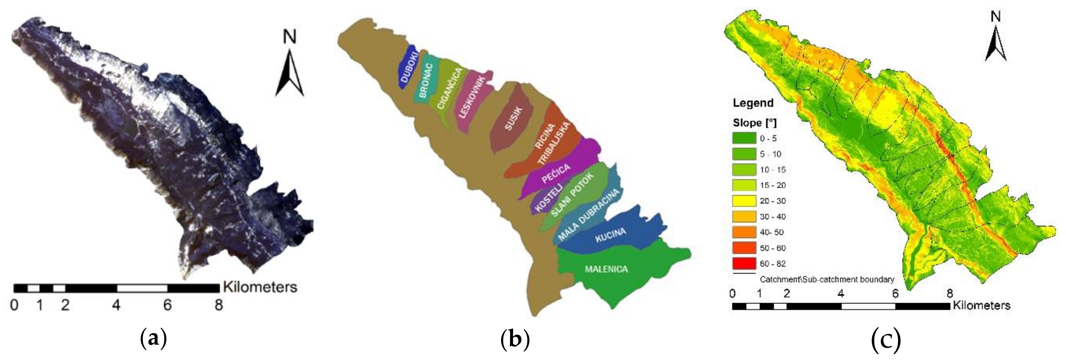
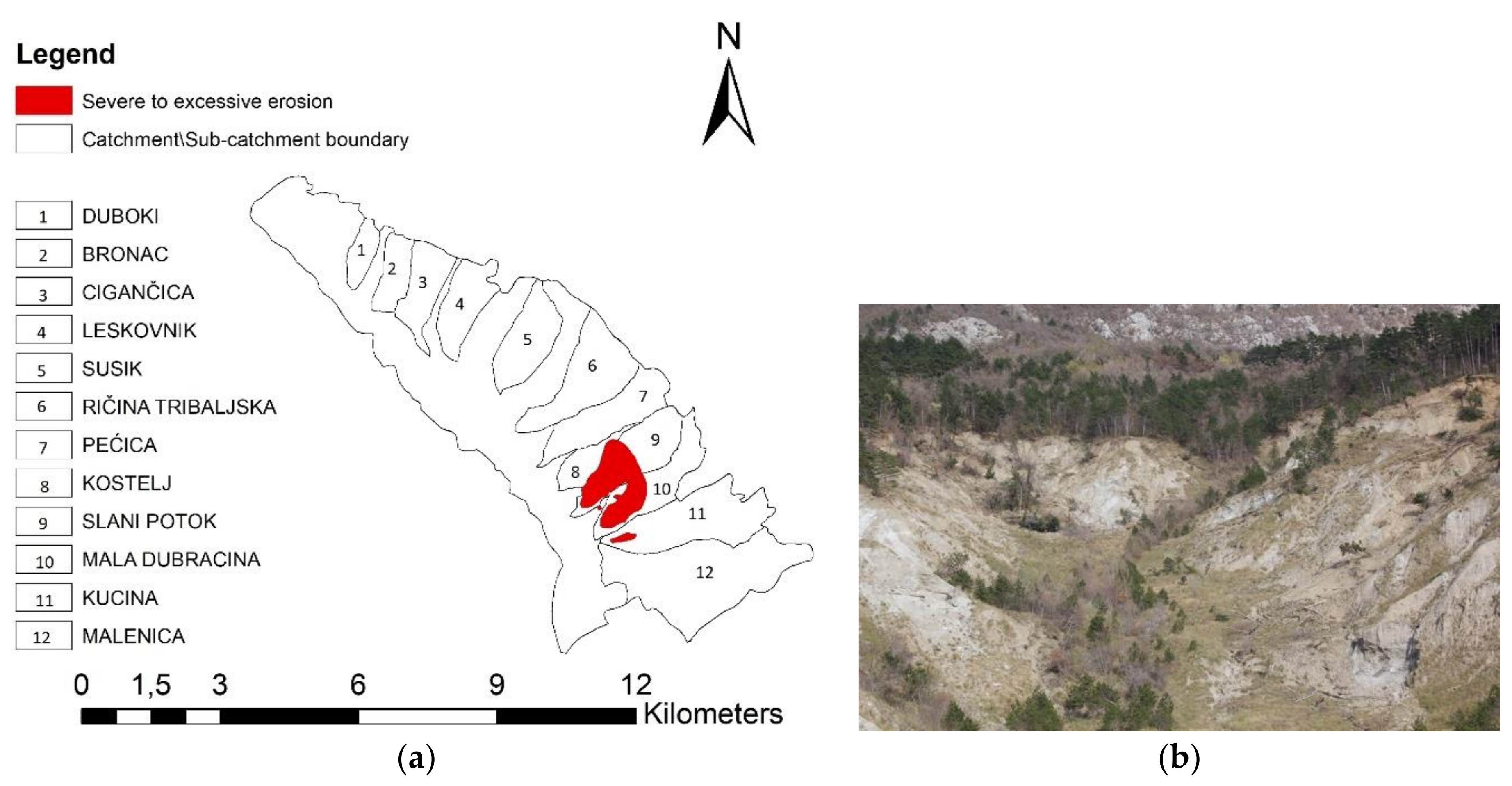
The analysis described in this paper is based on research and data gathered from the Dubračina Catchment area (Figure 1), which is situated in the Vinodol Valley in the County of Primorsko-Goranska, Croatia. The catchment area is 43.5 km2 in size. It has 12 small sub-catchments: Duboki, Bronac, Cigančica, Leskovnik, Sušik, Ričina Tribaljska, Pećica, Kostelj, Slani Potok, Mala Dubračina, Kučina, and Malenica. The catchment area is composed of karst and is characterised by steep slopes, active sediment movement and Flysch. Average annual rainfall is 1298 mm and the average temperature is 15 °C. The highest rainfall occurs during autumn, followed by winter, spring and summer. Through the years, the catchment was affected by erosion processes and multiple local landslides and flash floods. Today, approximately 3 km2 of its area is covered by excessive erosion (Figure 2). The type of erosion that prevails in the area is gully erosion. The most affected sub-catchments are Slani Potok and Mala Dubračina, where some roads and villages are highly endangered by erosion processes.
2.2. River Network
The Dubračina River catchment has 12 tributaries that form 12 small sub-catchments altogether. All tributaries, including the Dubračina River, have torrential characteristics. Most of the tributaries tend to dry out in the summer season but have oscillations in flow from autumn to spring.
For the purpose of deriving drainage density, two river network maps were extracted. The first river network map is based on a topographic map with a scale of 1:25,000 obtained from Spatial Plan of Vinodol Valley [35] dating from 2004. Based on the topographic map, the approximate length of the overall water network, including the Dubračina River, is 41 km (Table 1).
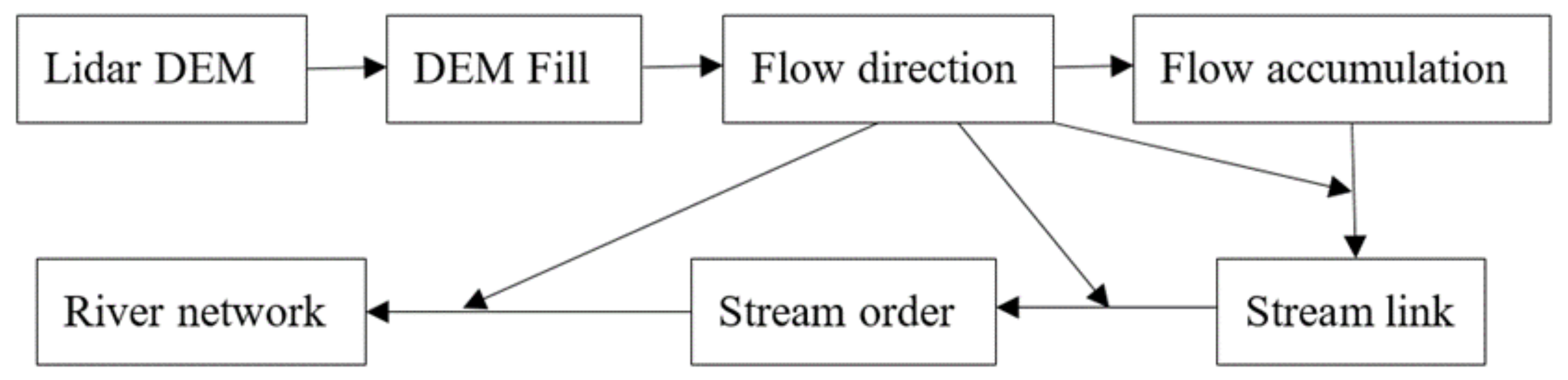
The second river network map was extracted from a Lidar (dated from 2012)-generated DEM with a resolution of 2 × 2 m (Table 2 and Figure 3). The DEM was analysed in GIS software (ArcGIS 10.5.1). The methods used for extracting the river networks consisted of filling sinks in the DEM and determined the flow direction, flow accumulation, stream links and stream order definitions (Figure 4).
A comparison of the two extracted river networks is presented in Figure 2. The overall length of the river network derived from the DEM is approximately 47.32 km, which is 15.4% longer than the river network based on the topographic map. The reason for this is the presence of gully erosion in the catchment. In these types of gullies, temporary surface flow occurs during high-intensity rainfall events. Gully erosion is one of the most erosive types of water erosion present worldwide and leads to land degradation that affects agricultural lands, sedimentation in rivers and lakes, and loss of livelihood and property damage [36].
Topographic map considers the primary and secondary rivers, but not gullies. Overall, the river network pattern derived from the DEM shows a 85% of similarity to the river network based on the topographic map. For this reason, both river networks are considered appropriate for further analysis, including the derivation of drainage density.
2.3. Drainage Density
When deriving drainage density (Equation (1)) for a catchment area, both perennial and intermittent rivers/tributaries need to be taken into consideration. If only perennial streams are included, the drainage density value for catchments with only intermittent streams would be equal to zero. In the case of a flood event, when both perennial and intermittent streams are active, its values would be unrealistic [1]:
where:
- L—Length of the waterway [km],
- N—Number of waterways,
- F—Contributing drainage area [km2].
Higher drainage density values indicate lower infiltration rates and higher surface flow velocity [37]. A high drainage density is often related to a high sediment yield transported through the river network, high flood peaks, steep hills, and a low suitability for agriculture.
Hydrogeological and geomorphological systems often have heterogeneous characteristics that vary with scale from microstructures to continents [13]. Drainage network patterns are no exception, and, consequently, nor is drainage density. The factors that influence drainage basin characteristics vary according to the scale of the input data (e.g., river network maps, digital elevation maps).
According to Gregory and Walling [8], the usefulness of drainage density as a model input parameter is limited by the method used to derive the drainage network, as well as the map and its scale that represents the catchment river network.
The drainage density for the Dubračina catchment was derived four times using different assumptions and spatial variabilities.
In the first case scenario, drainage density for the Dubračina catchment is derived with an assumption that the entire catchment is homogeneous and has no spatial variance in its characteristics, including drainage density. For the calculation, Equation (2) is used:
where lp is the length of the principal waterway, la is the cumulated length of the secondary waterways and F is the catchment area.
The second case scenario takes into consideration the variability of the sub-catchments. In this case, drainage density is calculated using the same equation (Equation (2)) for each sub-catchment separately.
In the third and fourth case scenarios, the drainage density is derived using the methodology proposed by Dobos and Daroussin [25]. They derived a potential drainage density map using ARCGIS software and a drainage network map derived from a DEM (90 m resolution SRTM DEM). They first assigned a value of one to each cell representing a drainage line. Subsequently, the drainage density map was derived as a function of the sums of all cell values that fall within a predefined shaped and sized neighbourhood (circle). The value for each pixel is then defined by moving the neighbourhood window and placing the desired pixel in the middle. Dobos and Daroussin [25] suggested the size and shape of the neighbourhood window to be variable for different case studies, depending on the current situation and user’s need. A minimum window size is needed in order to cover at least one drainage cell, which avoids having empty neighbourhoods and a value of zero for drainage density. In contrast, too large windows leads to a generalisation of the map since smaller windows maintain the physiographic patterns.
For the Dubračina catchment, some modifications to Dobos and Daroussin [25] methodology was made. First, square-shaped neighbourhood windows with a size of 1 × 1 km for a cell size of 1 × 1 m were used instead of a circle defined neighbourhood. A neighbourhood window with a size of 1 × 1 km was chosen to neutralise the value for the area in Equation (1), and thus, the drainage density for each cell is equivalent to the summation of all primary and secondary river lengths within the square window of 1 km2. Second, for the Dubračina catchment, the actual drainage density is calculated based on the river network map with a scale of 1:25,000 obtained from the Spatial Plan of Vinodol County [35]. This contradicts the case presented by Dobos and Daroussin [25], where potential drainage density was calculated based on a DEM-derived river network. For the fourth case scenario, potential drainage density was calculated based on a river network extracted from the Lidar DEM. Obtained Lidar has much better resolution (2 × 2 m) than 90 m SRTM DEM used by Dobos and Daroussin [25].
The categorisation of drainage density parameters used in this research is based on a proposed drainage density categorisation given by Ravi Shankar and Mohan [38] (Table 3).
The derived drainage density was used later as input data for the calculation of the sediment delivery ratio in the EPM intended for the soil erosion assessment in the Dubračina catchment area.
The approach used in both the first and second case scenario for deriving drainage density are continuously used in various case studies related to applications of the EPM [39]. For the purpose of determining the effect of different drainage density scales and derivation approaches on EPM, all four approaches were used and compared in the Results and Discussion section of the paper.
2.4. Erosion Potential Method
The EPM was developed in the 1960s for erosion assessments (Table 4) in the areas characterised by karst terrain and torrential watercourses. The method provides an assessment for the total annual volume of detached soil (Equation (3)), an erosion coefficient (Equation (5)) and actual sediment yield (Equation (7)) [39]. The parameter of drainage density only influences the third model outcome (actual sediment yield) through the sediment delivery ratio. For this reason, further analyses shown in this paper reflect only on the parameter sediment delivery ratio and its relation to estimating drainage density.
where:
- Wa—Total annual volume of detached soil [m3/year]
- T—Temperature coefficient [-]
- Pa—Average annual precipitation [mm]
- Z—Erosion coefficient [-]
- F—Study area [km2]
- T0—Average annual temperature [oC]
- Y—Soil erodibility coefficient [-]
- Xa—Soil protection coefficient [-]
- —Coefficient of type and extent of erosion [-]
- Ja—Average slope of the study area [%]
- ξ—Sediment delivery ratio [-]
- O—Perimeter of the study area [km]
- z—Mean difference in elevation of the study area [km]
- Dd—Drainage density [km/km2]
- lp—Length of the principal waterway [km]
- Gy—Actual sediment yield [m3/year]
3. Results and Discussion
The drainage density value (0.923 km/km2) obtained in the first case scenario corresponds to the very low drainage density class in Ravi Shankar and Mohan’s [38] drainage density classification and is homogenous throughout the entire catchment.
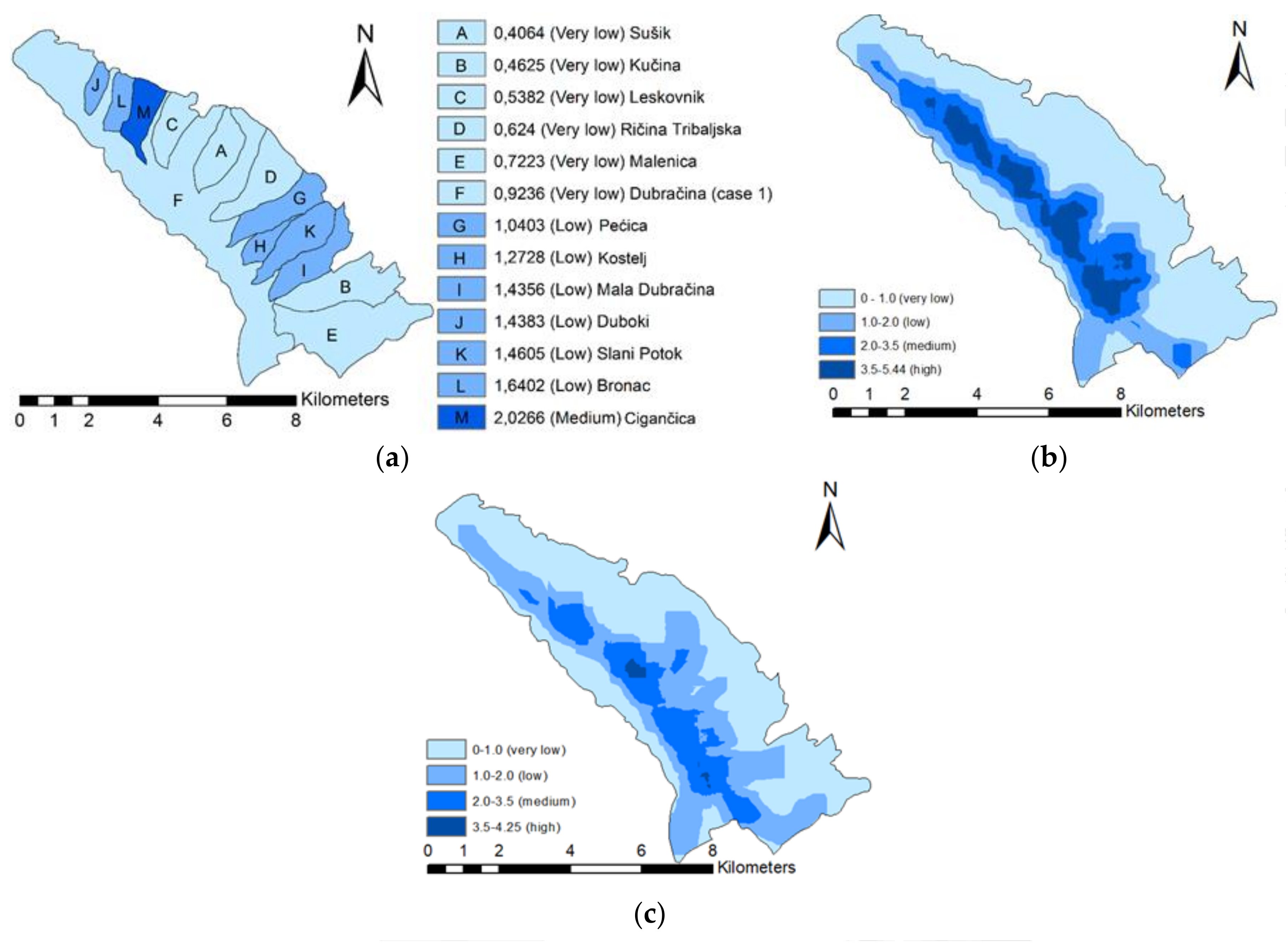
In the second case scenario (Figure 5), using the same classification, five sub-catchments within the Dubračina catchment have very low drainage densities (Sušik, Kučina, Leskovnik, Ričina and Malenica), while the six other sub-catchments have low values (Pećica, Kostelj, Mala Dubračina, Duboki, Slani Potok and Bronac), and only the Cigančica sub-catchment has a medium drainage density. It is known that low values for drainage density can indicate different characteristics, such as higher infiltration rates, lower surface flow velocities and/or lower values of sediment yield transported through river networks, all of which do not necessarily relate to the Slani potok and Mala Dubračina sub-catchments, which are two of the most severely affected sub-catchments by erosion processes (Figure 2).
Differences in spatial variability and drainage density values for the second, third and fourth case scenarios can be seen in Figure 5. Since the first case scenario represents a homogenous drainage density for the entire catchment, and current technological possibilities provide much more detailed and accurate maps, this case is disregarded from further analysis in this paper. Between the three other cases, the third and fourth case scenarios provide the most spatially variant maps and are the most complex maps to derive. In cases three and four, the obtained drainage density maps provide the most realistic spatial variance for this parameter, with lower drainage density values along the edges of the catchment and higher values concentrated along the river and tributary intersections where higher surface velocity, lower infiltration rates and higher values for sediment yield transport are expected. The difference between the third and fourth case scenarios is mainly at the river intersections, where the third case scenario results in higher drainage density values. The basic statistical analysis and comparison between the third and fourth case scenarios are given in Table 4 and Table 5.
Overall, the mean values for drainage density in fourth case scenario are lower for most sub-catchments, with the exception of five (Kostelj, Malenica, Kučina, Ričina Tribaljska and Sušik). For these sub-catchments, the maximum values are lower than in the third case scenario.
The statistical analysis, t-test with 95% confidence (two-tailed test), was conducted with a purpose to define if the difference between drainage density maps (case scenarios II to IV) is significant. The null hypothesis assumes that the two data sets (drainage density maps) are likely to have come from distribution with equal population means. Comparison was made in the pairs II–III, II–IV and III–IV case scenarios. Analysis has shown no significant change between the scenarios (Table 6).
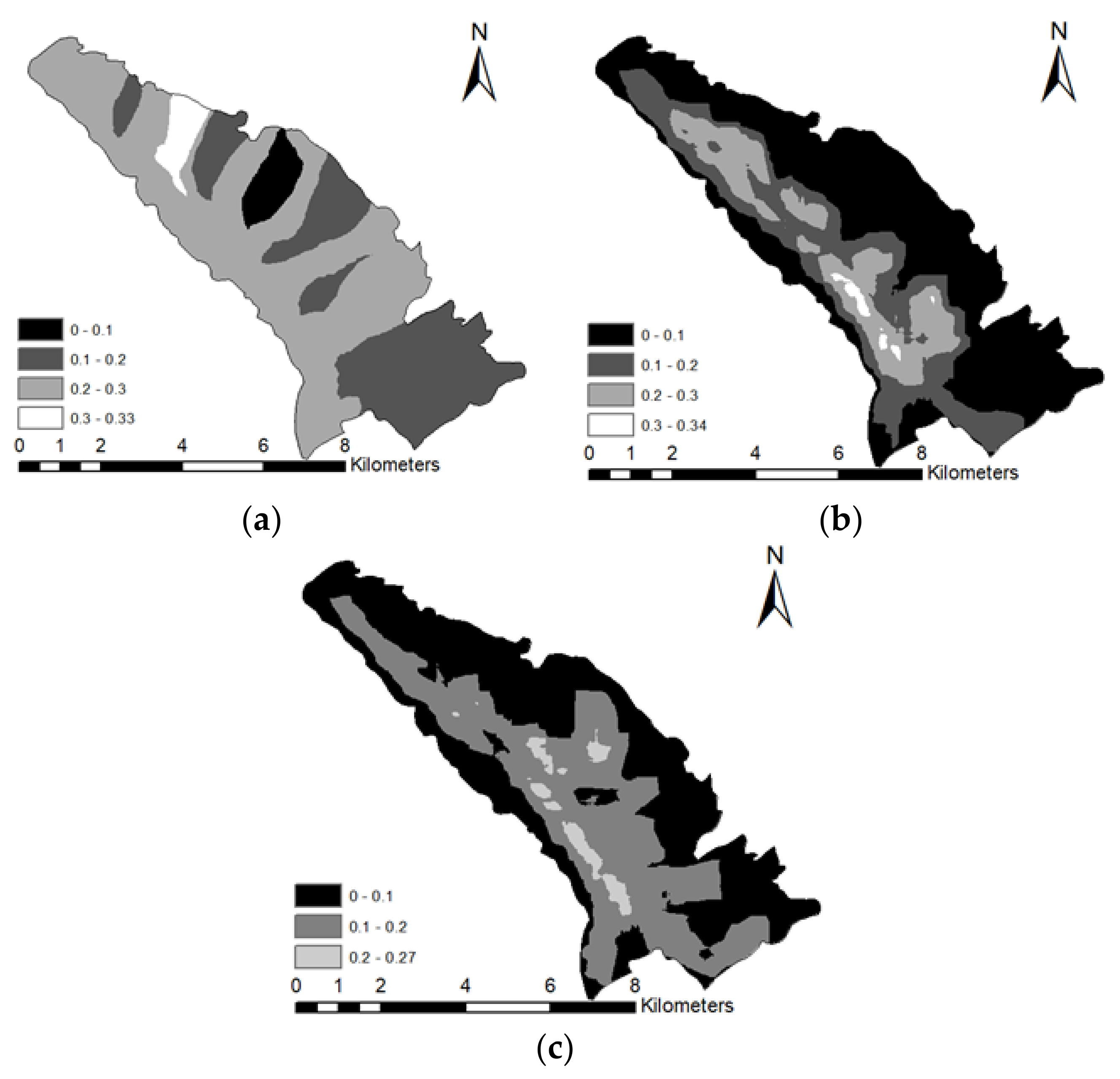
The question is, how do these four different drainage density derivation approaches affect the sediment delivery ratio in EPM? The main model parameter that is dependent on the drainage density parameter is the sediment delivery ratio ξ. This parameter was calculated for three case scenarios (Table 7 and Table 8, Figure 6) using Equation (6) and previously derived drainage maps shown in Figure 5 (case scenario II–IV) as input data.
The range of values for the second and third case scenarios do not differ much, but the spatial variation of the parameter is different, as can be seen in Figure 6, and it follows the same variation pattern as drainage density. Mean values for the fourth case scenario differ somewhat from the third case scenario, but the spatial distribution remains similar. It can be observed that all four case scenarios provide different values, but the third and fourth case scenarios are the most similar in values and spatial distribution. Therefore, the third and fourth case scenarios provide the best spatial variability for the drainage density parameter. This method was used in previous research by Dobos and Daroussin [25] and was approved and defined as an appropriate method for deriving drainage density maps. Thus, both case scenarios are considered appropriate input data for the EPM application in the Dubračina catchment.
The statistical analysis, t-test, was conducted once again, this time for the sediment delivery ratio, using the same assumptions and same pair comparisons (Table 9).
For the pairs II–III and II–IV, a significant change was found between derived datasets. But no significant change was found for the III–IV pair comparison.
4. Conclusions
The first case scenario provided no spatial variability and as such cannot be considered comparable to other case scenarios. Also, due to its homogenous characteristics throughout the catchment, it is considered less reliable and precise. For the derivation of drainage density for the III. and IV. case scenario, some modifications were made to the original methodology proposed by Dobos and Daroussin [25]. In both case scenarios, square neighbourhood windows were used opposite to the circle neighbourhood. In the third case scenario, actual drainage density was calculated using topographic maps as input data. The fourth case scenario used high resolution Lidar data as input data to derive potential drainage density map. However, according to Dobos and Daroussin [25], potential drainage density should always be higher or equal to actual drainage density, which is not the case in our analysis. The reason for that may be found in high resolution input data for the IV. case scenario. The topographic map for the Dubracina catchment is approximately 10 years older than the Lidar data, so some changes in the drainage patterns are expected to occur in this time period. This area, as it was mentioned before, is characterised by gully type of erosion and has intensive rainfall, all of which affects drainage patterns. For future analysis, detailed field observations and measurement should be conducted.
No significant difference was found between drainage density maps but they effect the sediment delivery ratio used in EPM. A significant change in sediment delivery ratio was found between II and III case scenarios and II and IV case scenarios. However, the change between drainage density maps was not considered significant; its effect on EPM parameter (sediment delivery ratio) should not be neglected.
The drainage density map, derived using the Dobos and Daroussin [25] methodology, has provided more realistic model input data with more detailed spatial variance of this parameter. The methods used in the third and fourth case scenarios have been applied for the first time in the EPM in the Dubračina catchment. Until now, drainage density that was used as input data in the EPM had a maximum spatial variability on the sub-catchment level, or was a unique value for the entire catchment. For this reason, the Dobos and Daroussin [25] modified methodology, used to derive drainage density maps for this case study, is considered an improvement in the accuracy and precision of the EPM.
Author Contributions
Conceptualization, N.D.; Data curation, N.D.; Formal analysis, N.D.; Funding acquisition, B.K. and N.O.; Investigation, N.D.; Methodology, N.D.; Project administration, N.D., B.K. and N.O.; Resources, N.D., B.K. and N.O.; Supervision, N.D., B.K. and N.O.; Validation, N.D., B.K. and N.O.; Visualization, N.D. and B.K.; Writing—original draft, N.D.; Writing—review & editing, B.K. and N.O.
Funding
“This research was funded by University of Rijeka, grant number 13.05.1.3.08. and 13.05.1.1.03.” and “The APC was funded by UNIRI-TECHNIC-18-129 and UNIRI-TEHNIC-18-54”.
Acknowledgments
This research was conducted within the University of Rijeka founded projects: Development of New Methodologies in Water and Soil Management in Karstic, Sensitive and Protected Areas (13.05.1.3.08) and Hydrology of water resources and risk identification of flooding and mudflows in the karst areas (13.05.1.1.03), Croatian-Japanese project Risk identification and Land-Use Planning for Disaster Mitigation of Landslides and Floods in Croatia, Implementation of Innovative Methodologies, Approaches and Tools for Sustainable River Basin Management (UNIRI-TEHNIC-18-129) and Water Resources Hydrology and Floods and Mud Flow Risks Identification in the Karstic Areas (UNIRI-TEHNIC-18-).
Conflicts of Interest
The authors declare no conflict of interest.
References
- Horton, R.E. Erosional development of streams and their drainage basins; hydrophysical approach to quantitative morphology. Geol. Soc. Am. Bull. 1945, 56, 275–370. [Google Scholar] [CrossRef]
- Glennon, A.; Groves, C. An examination of perennial stream drainage patterns within the Mammoth Cave watershed, Kentucky. J. Cave Karst Stud. 2002, 64, 82–91. [Google Scholar]
- Gallagher, A.S. Aquatic Habitat Assessment; American Fisheries Society Bethesda: Bethesda, MD, USA, 1999; pp. 25–34. ISBN 1-888569-18-2. [Google Scholar]
- Marani, M.; Belluco, E.; D’Alpaos, A.; Defina, A.; Lanzoni, S.; Rinaldo, A. On the drainage density of tidal networks. Water Resour. Res. 2003, 39. [Google Scholar] [CrossRef]
- Prabu, P.; Baskaran, R. Drainage Morphometry of Upper Vaigai River Sub-basin, Western Ghats, South India Using Remote Sensing and GIS. J. Geol. Soc. India 2013, 82, 519–528. [Google Scholar] [CrossRef]
- Abrahams, A.D. Channel networks: A geomorphological perspective. Water Resour. Res. 1984, 20, 161–188. [Google Scholar] [CrossRef]
- Collins, D.B.G.; Bras, R.L. Climatic and ecological controls of equilibrium drainage density, relief, and channel concavity in dry lands. Water Resour. Res. 2010, 46, W04508. [Google Scholar] [CrossRef]
- Gregory, K.J.; Walling, D.E. The variation of drainage density within a catchment. Hydrol. Sci. J. 1968, 13, 61–68. [Google Scholar] [CrossRef]
- Montgomery, D.R.; Dietrich, W.E. Source areas, drainage density, and channel initiation. Water Resour. Res. 1989, 25, 1907–1918. [Google Scholar] [CrossRef]
- Montgomery, D.R.; Dietrich, W.E. Channel Initiation and the Problem of Landscape Scale. Science 1992, 255, 826–830. [Google Scholar] [CrossRef] [PubMed]
- Dietrich, W.E.; Wilson, C.J.; Montgomery, D.R.; McKean, J. Analysis of Erosion Thresholds, Channel Networks, and Landscape Morphology Using a Digital Terrain Model. J. Geol. 1993, 101, 259–278. [Google Scholar] [CrossRef]
- Pallard, B.; Castellarin, A.; Montanari, A. A look at the links between drainage density and flood statistics. Hydrol. Earth Syst. Sci. 2009, 13, 1019–1029. [Google Scholar] [CrossRef]
- Luoto, M. New insights into factors controlling drainage density in subarctic landscapes. Arc. Antarct. Alpine Res. 2007, 39, 117–126. [Google Scholar] [CrossRef]
- Hadley, R.F.; Schumm, S.A. Sediment Sources and Drainage-Basin Characteristics in Upper Cheyenne River Basin; US Geological Survey: South Dakota, WY, USA, 1961.
- Tucker, G.E.; Bras, R.L. Hillslope processes, drainage density, and landscape morphology. Water Resour. Res. 1998, 34, 2751–2764. [Google Scholar] [CrossRef]
- Howard, A.D. Badland morphology and evolution: Interpretation using a simulation model. Earth Surface Processes Landforms 1997, 22, 211–227. [Google Scholar] [CrossRef]
- Tucker, G.E.; Catani, F.; Rinaldo, A.; Bras, R.L. Statistical analysis of drainage density from digital terrain data. Geomorphology 2001, 36, 187–202. [Google Scholar] [CrossRef]
- Lin, Z.; Oguchi, T. Drainage density, slope angle, and relative basin position in Japanese bare lands from high-resolution DEMs. Geomorphology 2004, 63, 159–173. [Google Scholar] [CrossRef]
- Rai, P.K.; Mohan, K.; Mishra, S.; Ahmad, A.; Mishra, V.N. A GIS-based approach in drainage morphometric analysis of Kanhar River Basin, India. Appl. Water Sci. 2017, 7, 217–232. [Google Scholar] [CrossRef]
- Ansari, Z.R.; Rao, L.A.K.; Yusuf, A. GIS based Morphometric Analysis of Yamuna Drainage Network in parts of Fatehabad Area of Agra District, Uttar Pradesh. J. Geol. Soc. India 2012, 79, 505–514. [Google Scholar] [CrossRef]
- Pal, S.; Saha, T.K. Exploring drainage/relief-scape sub-units in Atreyee river basin of India and Bangladesh. Spat. Inf. Res. 2017, 25, 685–692. [Google Scholar] [CrossRef]
- Asthana, A.K.L.; Gupta, A.K.; Luirei, K.; Bartarya, S.K.; Rai, S.K.; Tiwari, S.K. A Quantitative Analysis of the Ramganga Drainage Basin and Structural Control on Drainage Pattern in the Fault Zones, Uttarakhand. J. Geol. Soc. India 2015, 86, 9–22. [Google Scholar] [CrossRef]
- Sreedevi, P.D.; Sreekanth, P.D.; Khan, H.H.; Ahmed, S. Drainage morphometry and its influence on hydrology in an semi arid region: Using SRTM data and GIS. Environ. Earth Sci. 2013, 70, 839–848. [Google Scholar] [CrossRef]
- Strahler, A.N. Chow’s Handbook of Applied Hydrology; McGraw-Hill: New York, NY, USA, 1964; pp. 439–476. [Google Scholar]
- Dobos, E.; Daroussin, J. Potential drainage density Index (PDD). In An SRTM-Based Procedure to Delineate SOTER Terrain Units on 1:1 and 1:5 Million Scales; Office for Official Publications of the European Communities: Luxemburg, 2005; pp. 40–51. [Google Scholar]
- Ahmadi, H.; Das, A.; Pourtaheri, M.; Komaki, C.B.; Khairy, H. Redefining the watershed line and stream networks via digital resources and topographic map using GIS and remote sensing (case study: The Neka River’s watershed). Nat. Hazards 2014, 72, 711–722. [Google Scholar] [CrossRef]
- Al-Saady, Y.I.; Al-Suhail, Q.A.; Al-Tawash, B.S.; Othman, A.A. Drainage network extraction and morphometric analysis using remote sensing and GIS mapping techniques (Lesser Zab River Basin, Iraq and Iran). Environ. Earth Sci. 2016, 75, 1243. [Google Scholar] [CrossRef]
- Das, S. Geomorphic characteristics of a bedrock river inferred from drainage quantification, longitudinal profile, knickzone identification and concavity analysis: A DEM-based study. Arabian J. Geosci. 2018, 11, 680. [Google Scholar] [CrossRef]
- Gartsman, B.I.; Shekman, E.A. Potential of river network modeling based on GIS technologies and digital elevation model. Russ. Meteorol. Hydrol. 2016, 41, 63–71. [Google Scholar] [CrossRef]
- Kumar, B.; Patra, K.C.; Lakshmi, V. Error in Digital Network and Basin Area Delineation using D8 method: A Case Study in a Sub-basin of the Ganga. J. Geol. Soc. India 2017, 89, 65–70. [Google Scholar] [CrossRef]
- Siddiqui, S.; Castaldini, D.; Mauro, S. DEM-based drainage network analysis using steepness and Hack SL indices to identify areas of differential uplift in Emilia–Romagna Apennines, northern Italy. Arabian J. Geosci. 2017, 10, 1–23. [Google Scholar] [CrossRef]
- Tan, M.L.; Ramli, H.P.; Tam, T.H. Effect of DEM Resolution, Source, Resampling Technique and Area Threshold on SWAT Outputs. Water Resour. Manag. 2018, 32, 4591–4606. [Google Scholar] [CrossRef]
- Tebano, C.; Pasanisi, F.; Grauso, S. QMorphoStream: Processing tools in QGIS environment for the quantitative geomorphic analysis of watersheds and river networks. Earth Sci. Inf. 2017, 10, 257–268. [Google Scholar] [CrossRef]
- Dragičević, N.; Karleuša, B.; Ožanić, N. Improvement of Drainage Density Parameter Estimation within Erosion Potential Method; Multidisciplinary Digital Publishing Institute: Basel, Switzerland, 2018; Volume 2, p. 620. [Google Scholar]
- Spatial Plan of Area of Significance of Vinodol County. Available online: http://www.sn.pgz.hr/default.asp?Link=odluke&id=2414 (accessed on 5 March 2019).
- Nicu, I.C. Is Overgrazing Really Influencing Soil Erosion? Water 2018, 10, 1077. [Google Scholar] [CrossRef]
- Yalcin, A. GIS-based landslide susceptibility mapping using analytical hierarchy process and bivariate statistics in Ardesen (Turkey): Comparisons of results and confirmations. CATENA 2008, 72, 1–12. [Google Scholar] [CrossRef]
- Shankar, M.N.R.; Mohan, G. Assessment of the groundwater potential and quality in Bhatsa and Kalu river basins of Thane district, western Deccan Volcanic Province of India. Environ. Geol. 2006, 49, 990–998. [Google Scholar] [CrossRef]
- Dragičević, N.; Karleuša, B.; Ožanić, N. A review of the Gavrilović method (Erosion Potential Method) application. Građevinar 2016, 68, 715–725. [Google Scholar]
Figure 1.
Case study: (a) Dubračina catchment; (b) sub-catchments [34]; (c) slope in degrees derived from DEM.
Figure 1.
Case study: (a) Dubračina catchment; (b) sub-catchments [34]; (c) slope in degrees derived from DEM.

Figure 2.
Erosion affected areas: (a) map of areas affected by severe to excessive erosion processes; (b) excessive erosion processes on Slani Potok sub-catchment.
Figure 2.
Erosion affected areas: (a) map of areas affected by severe to excessive erosion processes; (b) excessive erosion processes on Slani Potok sub-catchment.

Figure 3.
River network based on different data source: (a) topographic map; (b) Lidar DEM.

Figure 4.
Methods for river network extraction from Lidar generated DEM.

Figure 5.
Drainage density for the Dubračina catchment: (a) Scenario II: sub-catchment; (b) Scenario III: topography map based; (c) Scenario IV: DEM derived river network based.
Figure 5.
Drainage density for the Dubračina catchment: (a) Scenario II: sub-catchment; (b) Scenario III: topography map based; (c) Scenario IV: DEM derived river network based.

Figure 6.
Sediment delivery ratio: (a) Scenario II: sub-catchment; (b) Scenario III: topographic map based; (c) Scenario IV: DEM-derived river network-based.
Figure 6.
Sediment delivery ratio: (a) Scenario II: sub-catchment; (b) Scenario III: topographic map based; (c) Scenario IV: DEM-derived river network-based.


Table 1.
Characteristics of the Dubračina River catchment and its sub-catchments [34].
Table 1.
Characteristics of the Dubračina River catchment and its sub-catchments [34].
| Tributary | Area (km2) | River Length | |
|---|---|---|---|
| [km] | [%] | ||
| Duboki | 0.67 | 0.96 | 2 |
| Bronac | 0.99 | 1.62 | 4 |
| Cigančica | 1.49 | 3.03 | 7 |
| Leskovnik | 1.62 | 0.87 | 2 |
| Susik | 1.93 | 0.78 | 2 |
| Ricina Tribaljska | 2.74 | 1.71 | 4 |
| Pećica | 2.23 | 2.32 | 6 |
| Kostelj | 0.82 | 1.04 | 3 |
| Slani Potok | 2.21 | 3.22 | 8 |
| Mala Dubracina | 2.09 | 3.00 | 7 |
| Kucina | 3.29 | 1.52 | 4 |
| Malenica | 5.54 | 4.00 | 10 |
| Dubracina River | 43.56 | 13.69 | 33 |
| Small unnamed tributaries | 3.23 | 8 | |
| Summarized | 40.99 | 100.00 | |
Table 2.
Data sources and resolutions used for river network extraction.
| Data | Resolution/Scale | Source |
|---|---|---|
| Digital elevation map | 2 m | Lidar data |
| Topographic map | 1:25,000 | Spatial plan of Vinodol Valley |
Table 3.
Categorisation of drainage density given by Ravi Shankar and Mohan [38].
Table 3.
Categorisation of drainage density given by Ravi Shankar and Mohan [38].
| Category | Very Low | Low | Medium | High |
|---|---|---|---|---|
| [km/km2] | <1.0 | 1.0–2.0 | 2.0–3.5 | >3.5 |
Table 4.
Descriptive statistics of drainage density for the Dubračina catchment.
| Drainage Density Based on | Min | Mean | Max | Stdev |
|---|---|---|---|---|
| Topographic map (Case scenario III) | 0 | 1.23 | 5.446 | 1.40 |
| Lidar generated DEM (Case scenario IV) | 0 | 1.02 | 4.253 | 0.908 |
Table 5.
Descriptive statistics of drainage density for the Dubračina sub-catchments.
| Sub-Catchment | Topographic Map—Based (III Case Scenario) | DEM—Based (IV Case Scenario) | ||||||
|---|---|---|---|---|---|---|---|---|
| Min | Mean | Max | Stdev | Min | Mean | Max | Stdev | |
| Duboki | 0 | 1.0 | 3.3 | 1.0 | 0 | 0.3 | 1.8 | 0.5 |
| Bronac | 0 | 1.6 | 4.6 | 1.5 | 0 | 0.5 | 2.2 | 0.6 |
| Cigančica | 0 | 1.7 | 5.0 | 1.7 | 0 | 0.8 | 3.2 | 0.9 |
| Leskovnik | 0 | 0.6 | 4.0 | 1.0 | 0 | 0.5 | 3.1 | 0.8 |
| Sušik | 0 | 0.5 | 4.2 | 1.0 | 0 | 0.7 | 3.5 | 0.8 |
| Ričina Tribaljska | 0 | 0.7 | 4.3 | 1.2 | 0 | 1.1 | 3.1 | 0.8 |
| Slani potok | 0 | 1.4 | 4.6 | 1.5 | 0 | 0.8 | 2.9 | 0.9 |
| Mala Dubračina | 0 | 1.7 | 4.9 | 1.6 | 0 | 0.9 | 3.6 | 1.0 |
| Kučina | 0 | 0.6 | 4.9 | 1.0 | 0 | 0.8 | 3.7 | 0.7 |
| Pećica | 0 | 1.0 | 5.3 | 1.6 | 0 | 0.9 | 3.2 | 0.6 |
| Malenica | 0 | 0.8 | 4.7 | 1.0 | 0 | 1.1 | 3.7 | 0.8 |
| Kostelj | 0.028 | 2.0 | 4.0 | 0.9 | 0.7 | 2.1 | 2.5 | 0.6 |
Table 6.
t-test results for the drainage density maps.
| II–III Case Scenario | II–IV Case Scenario | III–IV Case Scenario |
|---|---|---|
| p-value (0.829) > α (0.05) | p-value (0.304) > α (0.05) | p-value (0.208) > α (0.05) |
Table 7.
Sediment delivery ratio values for cases scenario II to IV for the Dubračina catchment.
| Case Scenario | II. Case (Mean Values) | III. Case (Mean Values) | II. Case (Mean Values) |
|---|---|---|---|
| Sediment delivery ratio | 0.1948 | 0.0091 | 0.0847 |
Table 8.
Descriptive statistics for the sediment delivery ratio for cases II to IV.
| Sub-Catchment | Sediment Delivery Ratio ξ | ||
|---|---|---|---|
| II. Case | III. Case (Mean Values) | IV. Case (Mean Values) | |
| Duboki | 0.1909 | 0.1075 | 0.0349 |
| Bronac | 0.2407 | 0.1268 | 0.0462 |
| Cigančica | 0.3291 | 0.1242 | 0.0582 |
| Leskovnik | 0.1112 | 0.0489 | 0.0418 |
| Sušik | 0.0853 | 0.0447 | 0.0728 |
| Ričina Tribaljska | 0.1379 | 0.0510 | 0.1056 |
| Slani potok | 0.2665 | 0.1118 | 0.0748 |
| Mala Dubračina | 0.2886 | 0.1244 | 0.0672 |
| Kučina | 0.1126 | 0.0462 | 0.0748 |
| Pećica | 0.2204 | 0.0748 | 0.0812 |
| Malenica | 0.1649 | 0.0592 | 0.0930 |
| Kostelj | 0.1903 | 0.1134 | 0.1480 |
Table 9.
t-test results for the sediment delivery ratio maps.
| II–III Case Scenario | II–IV Case Scenario | III–IV Case Scenario |
|---|---|---|
| p-value (0.000187) < α (0.05) | p-value (4.91 × 10⁻⁵) < α (0.05) | p-value (0.412) > α (0.05) |
© 2019 by the authors. Licensee MDPI, Basel, Switzerland. This article is an open access article distributed under the terms and conditions of the Creative Commons Attribution (CC BY) license (http://creativecommons.org/licenses/by/4.0/).
Share and Cite
MDPI and ACS Style
Dragičević, N.; Karleuša, B.; Ožanić, N. Different Approaches to Estimation of Drainage Density and Their Effect on the Erosion Potential Method. Water 2019, 11, 593. https://doi.org/10.3390/w11030593
AMA Style
Dragičević N, Karleuša B, Ožanić N. Different Approaches to Estimation of Drainage Density and Their Effect on the Erosion Potential Method. Water. 2019; 11(3):593. https://doi.org/10.3390/w11030593
Chicago/Turabian StyleDragičević, Nevena, Barbara Karleuša, and Nevenka Ožanić. 2019. "Different Approaches to Estimation of Drainage Density and Their Effect on the Erosion Potential Method" Water 11, no. 3: 593. https://doi.org/10.3390/w11030593
Note that from the first issue of 2016, this journal uses article numbers instead of page numbers. See further details here.