1. Introduction
In the Arctic and sub-Arctic, climate change leads to permafrost thaw, which in turn changes hydrological flow variability [
1,
2] and pathways (stretches and times) of waterborne carbon, nutrient, and pollutant spreading [
3]. Permafrost thaw also relates to thermokarst wetland lake formation and/or drainage (
Figure 1) and associated ecosystem regime shifts [
4]. The right-hand loop in the system diagram for linked permafrost and thermokarst wetland/lake changes shown in
Figure 1 prevails when there is relatively shallow permafrost thaw, leading to thermokarst formation with an increase of wetlands and lakes at the land surface. The left-hand loop in
Figure 1 prevails when permafrost thaw goes deeper, leading to taliks (unfrozen soil zones and conduits) that increase drainage and thereby decrease the prevalence of wetlands and lakes at the surface. The conditions of permafrost thaw and its depth extent, hence, represent a bifurcation point (division into two behavior branches) of vital importance for wetland/lake prevalence and evolution under warming in Arctic/sub-Arctic permafrost regions.
In combination with these effects on thermokarst wetlands and lakes, the thawing of permafrost under warming also presents further challenges to mankind for a variety of reasons. These include climate feedbacks by carbon release into the atmosphere [
5] (also related to wetlands as indicated in
Figure 1), as well as impacts on infrastructure [
6] and ecology [
7]. Permafrost also serves as a natural bank for a variety of organic material, dormant propagules (seeds, eggs, cysts, or spores from plants and invertebrates), and other viable vectors (bacteria, viruses) [
8]. Thawing of permafrost may then lead to re-emergence of these with increased risks to health and wellbeing for animals and humans [
8,
9,
10,
11]. These risks may be further raised by thaw-driven increases of water discharges [
12] and associated loading of dissolved organic matter (DOM) to surface waters [
13], leading to increased selective absorption of ultraviolet radiation by DOM and, thereby, decreased sunlight inactivation of pathogens in these waters [
14].
The permafrost in the northern circumpolar region has been warming in recent decades [
15]. There is now great and urgent need to quantify and predict permafrost evolution under ongoing and future warming conditions, as basis for also assessing the evolution of thermokarst wetlands and lakes, climate feedback, and societal, ecological, and health risks. Permafrost degradation is not expected to diminish in the future; a recent study [
16] concluded that if the climate is stabilized at 2 °C above pre-industrial levels (COP21 climate change target), the global permafrost area may be reduced by over 40% relative to a 1960–1990 baseline, with severe impacts also on thermokarst wetlands-lakes. However, global climate models (e.g., in the Coupled Model Intercomparison Project phase 5 (CMIP5) database) result in a wide range of predictions, reflecting large uncertainty for this evolution under warming [
17,
18].
In addition to large-scale surface warming, local conditions in the landscape, which are not resolved very well by climate models, also influence permafrost thaw [
19,
20,
21,
22], associated wetland-lake evolution, and societal and health risks. Regarding influences on landscape conditions, including the evolution of thermokarst lakes and wetlands, local soil and hydrogeological differences may be essential for the spatial variability of permafrost thaw under the same large-scale surface temperature [
1]. Great spatiotemporal complexity is also suggested for the evolution of permafrost peatlands under warming [
23], and there is ongoing debate about the potential protection of permafrost against thawing by sand layer or dune formation over the frozen ground (desertification) [
24,
25]. Local elevation conditions also influence the permafrost dynamics and, in resolving the permafrost thaw complexity, low elevation and southern sites may be particularly useful as relatively early representatives of forthcoming warming effects.
In general, how large-scale surface warming interacts with local landscape conditions in determining where, and to what degree, permafrost thaws is a key research question for improved understanding of the thawing itself, and for our ability to further assess the evolution of thermokarst wetland-lake ecosystems and related societal and health risks in permafrost regions. This study addresses this question through systematic simulations of different local soil-permafrost formations combined with different large-scale surface warming trends.
2. Materials and Methods
The present simulations were carried out with the numerical tool DarcyTools, representing water flow and heat transport [
26,
27] and associated permafrost formation/degradation [
28,
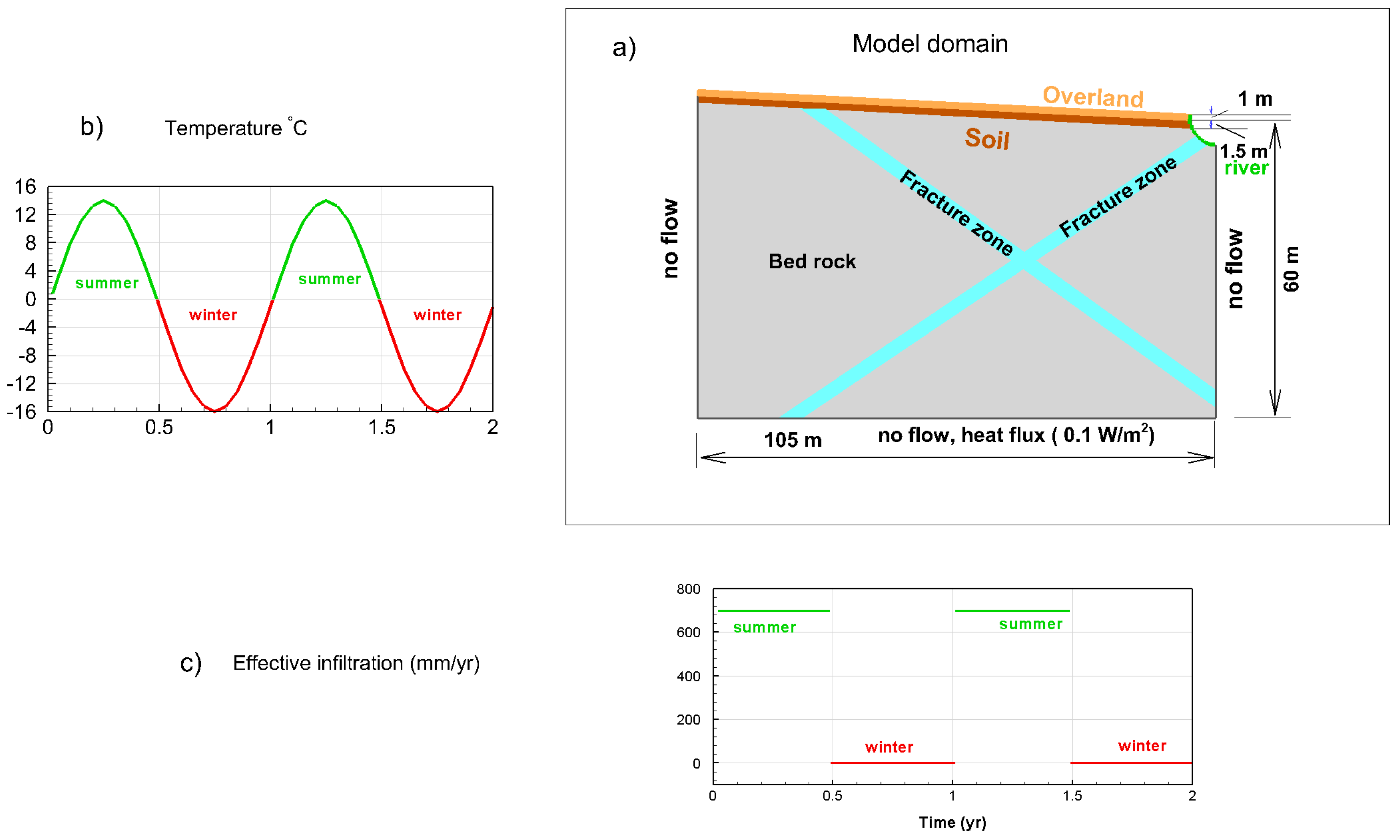
29] in a generic model domain (
Figure 2a). The domain follows previous systematic simulation studies in the literature [
1,
3,
12,
30,
31] of two-dimensional surface/subsurface cross-sections. It has water recharging at the top boundary and discharging into a downgradient river at the right-hand boundary. In general, a river will act to maintain talik-like conditions in its close proximity.
DarcyTools [
26,
27] is a flexible numerical simulation tool, representing time-variable groundwater flow (and groundwater table, thus also representing the time-variable unsaturated zone extent) and heat transport (as well as solute transport, a feature not used in the present study). In DarcyTools simulations, the permafrost dynamics is handled numerically, as described in detail by [
28,
29], and summarized here further below. The combined groundwater flow, heat transport, and phase change functionality in DarcyTools has been verified in a cross-code comparison study [
31]. In
Section 3 (Results) and
Section 4 (Discussion) below in this paper, we also outline how the present simulations using the DarcyTools modelling software capture key field-observed aspects of permafrost conditions in different parts of the high-latitude permafrost region.
DarcyTools handles permafrost, with the method first presented by [
32], by changing the relation between ice and water contents within the available pore space (kinematic porosity), and by assigning low hydraulic conductivity values for soil domain parts with a temperature below a specified threshold (typically 0 °C). Empirical functions represent the relationships of temperature–ice content–hydraulic conductivity [
28,
29]. In the present application, a maximum permafrost reduction factor of 0.05 was used, implying that fully frozen ground will have a hydraulic conductivity that is 5% of its original, unfrozen value. Ground ice, referring to ice existing in amounts exceeding soil porosity in the form of ice lenses and wedges, is not accounted for in DarcyTools. However, other simulations have shown that such ground ice merely may delay permafrost thaw by reducing soil warming without changing the essential thaw outcome [
33]. Also, surface subsidence resulting from permafrost thaw is not accounted for in DarcyTools. Not accounting for these processes is deemed not vital for the scope and comparative purposes of the present generic simulations, as numerous previous simulation studies of permafrost thaw also have not included these types of processes [
1,
3,
12,
34,
35].
In the present simulations, a sinusoidal intra-annual variation of surface temperature (range −16–14 °C in the case with no warming trend,
Figure 2b) and an effective infiltration rate (precipitation minus evapotranspiration,
Figure 2c) were applied at the top boundary of the model domain (
Figure 2a). The applied effective infiltration rate was zero when the temperature was negative, and it was uniform at 700 mm/year at times with positive surface temperature (
Figure 2c). Since half of each year has negative temperatures, the total annual effective infiltration in the simulations was 350 mm/year. This annual average rate implicitly accounts for, and is on average consistent with, the annual average precipitation and evapotranspiration rates of multiple drainage basins across the circum-polar permafrost region [
36]. Specifically, these annual rates are on average around 550 mm/year for precipitation and 200 mm/year for evapotranspiration [
36], thus implying the annual average effective infiltration rate of around the 350 mm/year that we have applied at the surface of the present simulation domain. In these terms, this may be viewed as representative of a lateral plane just below the soil root zone. Remaining domain boundaries were no-flow with regard to water and heat, except for the top of the right-hand boundary where water discharged into a river and the lower boundary where a constant heat flux of 0.1 W/m
2 was applied to represent the geothermal heat transport. The river had a specified pressure; thus, the effective infiltration rate through the top boundary was forced to discharge through the river.
The present simulation study aims to identify and compare key patterns and differences in permafrost prevalence and thaw for different generic types of local soil/rock conditions combined with large-scale surface temperature/warming and hydrological (effective infiltration) conditions. As such, in the simulations we focused on representing overarching, large-scale forcings that are consistent with observed annual and seasonal average hydro-climatic conditions (in terms of surface temperature/warming and effective infiltration) rather than simulating details of these variables, or of any additional conditions and their variability (e.g., snow depth and its degree of insulation, vegetation, and associated effects on evapotranspiration rate and soil organic matter, or peat erosion/accumulation). All these conditions and variabilities are site-specific and highly variable across the permafrost region, and we do not aim here to simulate any particular site situation within this region.
Furthermore, as warming can be expected to be dominant in driving permafrost thaw, we focused the simulations on different temperature trend scenarios rather than also considering other types of large-scale hydro-climatic trends, such as in effective infiltration rate as some combined effect of trends in precipitation and evapotranspiration. Basic seasonal variation in effective infiltration rate was represented in the simulations by the different actual rates applied at the upper domain boundary (zero when temperature was negative, 700 mm/year when temperature was positive;
Figure 2c) to get the observation-consistent annual average rate of 350 mm/year. The overarching working hypothesis underlying these study choices is that such schematic generic simulations of main large-scale warming forcing, combined with different types of local soil/rock conditions, will still be able to capture main patterns and differences in permafrost prevalence and thaw for different local conditions. In obtaining the simulation results, we further compared and tested this hypothesis against corresponding field observation reports; this comparison is done in
Section 3 (Results) and
Section 4 (Discussion).
In general, the modelled formation and thaw of permafrost is temperature-dependent, and groundwater flow through the modelled system depends on both the applied effective infiltration rate and the permafrost conditions that are governed by the developed subsurface temperature field, which in turn depended on both heat convection and advection of heat by the flowing groundwater. Thus, the simulation of water-heat transport and permafrost formation-change is normally fully coupled, except for the sensitivity/robustness test cases considering only heat conduction or only waterborne convection–advection in the present simulations.
The first simulation step with no warming trend at the surface was started from a system free of permafrost, to which we applied the above described repeated intra-annual variation in surface temperature and effective infiltration. In this first simulation step, the driving forces are such that permafrost develops over time from more or less arbitrary initial conditions, with no warming trend at the surface and a repeated annual freezing/thawing cycle. Once a pseudo-steady state with equilibrium average conditions is achieved (i.e., changes in annual average flow between consecutive years are small under the applied constant average surface temperature (achieved well within 100 years of simulation time), we continued simulations with the second phase, applying a warming trend at the surface of either a 1 °C increase or a 2 °C increase linearly over 100 years. The simulations used a time step of 0.02 years, with 20 sweeps (iterations) per time step to ensure convergence.
Spatially, the two-dimensional simulation domain had vertical and horizontal extents of approximately 60 m by 105 m (
Figure 2a). The top surface sloped towards the right-hand top corner of the domain. The domain was divided into separate units consisting of a single or several soil layers, fractured bedrock, and fracture zones beneath the soil layer. An overland flow unit was located on top of the top-most soil layer. The maximum cell size was 1 m × 1 m in the bedrock, and 0.25 m × 0.25 m closer to the top surface. In total, there were about 16,000 cells.
The simulation set-up included representation of the unsaturated zone, implying that the simulated groundwater table fluctuated during the year. Specifically, during the winter period when effective infiltration was zero, the groundwater table dropped and resulted in a smaller hydraulic gradient toward the river. Conversely, during the summer period when effective infiltration was greater than zero, the groundwater table rose, and the hydraulic gradient towards the river increased. The simulation configuration was such in terms of effective infiltration rate, surface slope, and parameterization that the groundwater table never rose above ground surface.
The chosen rock properties were representative of crystalline rock (i.e., the bedrock is fairly tight with low porosity, but fracture zones of higher hydraulic conductivity and porosity intersected the bedrock, as reported in
Table 1). The upper soil layers were chosen to have higher hydraulic conductivity than both the fracture zones and the bedrock, and also higher porosity than the bedrock; in line with the present generic simulations, these values are not site-specific, but chosen to reflect some realistic types of local property differences between some typical geologic materials. Furthermore, the overland layer was given a high enough hydraulic conductivity in the horizontal direction that flow in excess of the physically possible groundwater recharge (determined by the effective infiltration rate) was instead directed laterally towards the river.
Concerning thermal properties, the mineral soil was assigned thermal properties equal to the bedrock, whereas the peat soil was assigned lower thermal conductivity (
Table 1). The fracture zones had properties in between those of the bedrock and the peat soil. Concerning the heat capacity, the order was reversed; the peat soil had the highest value, followed by the fracture zones, and the bedrock. The overland layer was assigned thermal properties equal to peat (
Table 1). Storativity followed a depth trend with a value of 0.1 m
−1 at the surface and a value of 1 × 10
−9 m
−1 at 8 m depth. Below this depth, storativity was held constant at 1 × 10
−9 m
−1. The river and the overland layer were always maintained ice-free by being assigned a constant temperature of 1 °C.
3. Results
A first simulation step without any warming trend (i.e., for average surface temperature of −1 °C;
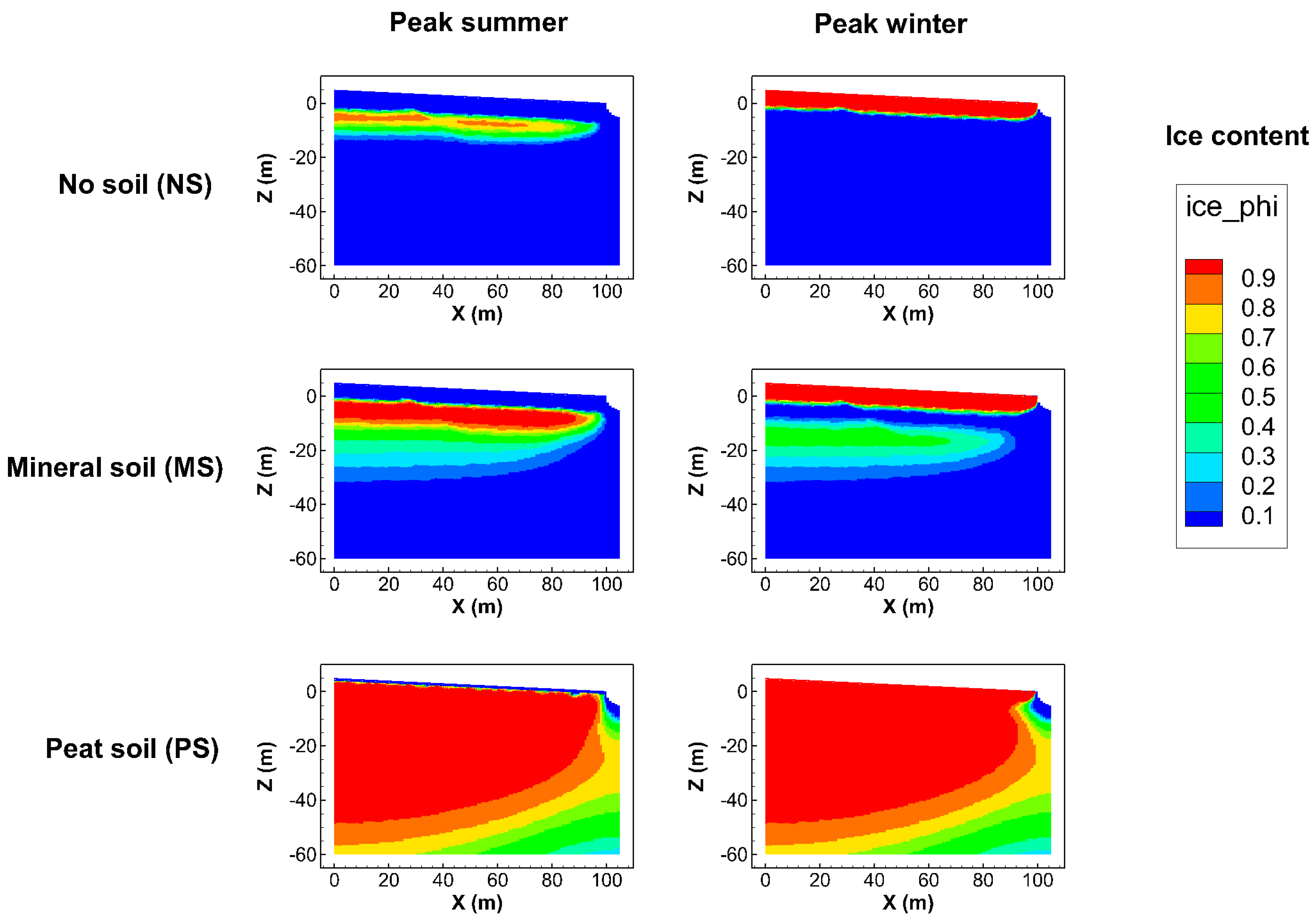
Figure 2b) led to different ice content conditions for different soil permafrost cases (
Table 1), as illustrated in
Figure 3 for the times of peak summer and peak winter (see
Figure 2b,c for the temperature and effective infiltration conditions at these times). This simulation was started without any permafrost in the model domain and was continued until the intra-annual variation was the same from year to year (i.e., until pseudo-steady state conditions were reached) for each soil permafrost case.
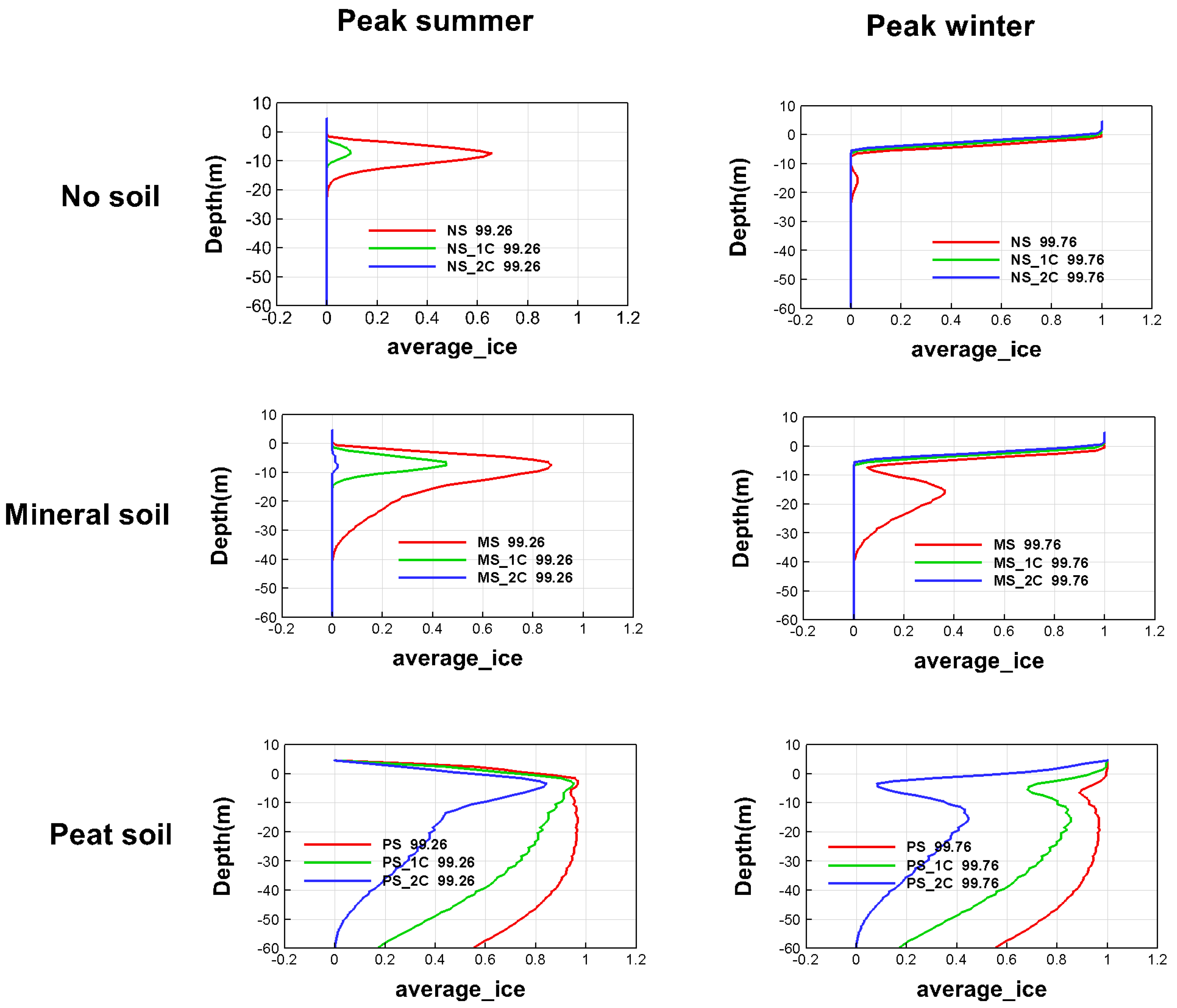
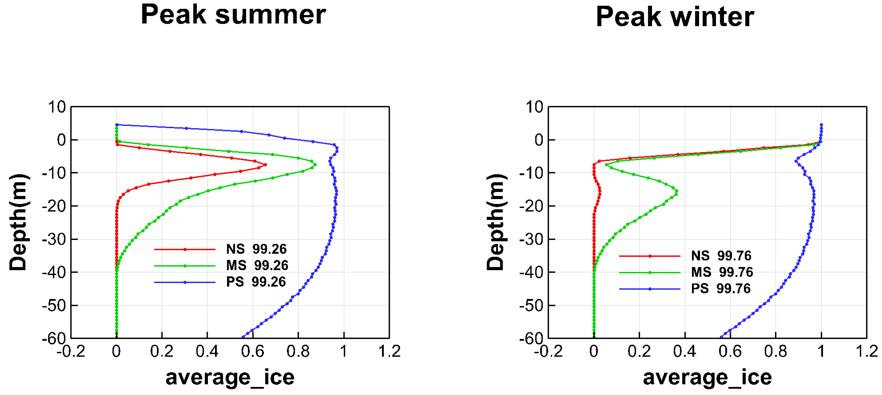
Figure 3 shows widely different ice and permafrost conditions in the subsurface under the same hydro-climatic conditions at surface. In the case with no soil cover on top of the bed rock (NS), only a thin ice zone some few meters under the surface remained as a permafrost layer during peak summer, while the peat soil case (PS) had almost the same, full ice content extending over nearly the whole model domain in peak summer as in peak winter. The mineral soil case (MS) was intermediate in this regard, but it was much more similar to the NS than the PS case. These conditions and main differences among the considered soil-permafrost cases at quasi-steady-state are also illustrated in terms of lateral average ice content as a function of depth, as shown in
Figure A1 of the
Appendix.
The PS case, thus, involves much more subsurface ice and permafrost extending over a greater depth than the mutually more similar MS and NS cases. This result is consistent with the MS and NS cases having the same thermal properties (thermal conductivity and heat capacity), which in turn differ from those in the PS case (
Table 1). These property differences and ice-content results suggest that the process of conductive heat transport, governed by the thermal properties, as the dominant heat transport mechanism in the simulated cases. In further consistency with this implication, the MS and PS cases have the same hydraulic properties (hydraulic conductivity and porosity) but widely different ice-content results, which also suggests the process of convective–advective heat transport, governed by the hydraulic properties, as less important than heat conduction for the ice content prevailing in the simulated cases.
Multiple field observations support the main result featured in these simulations: that permafrost prevalence and extent, for the same large-scale surface temperature conditions (and the same hydrology, in terms of effective infiltration, i.e., precipitation minus evapotranspiration), are strongly linked with local peat occurrence. For example, in continental western Canada, the percentage of localized permafrost in discontinuous permafrost areas has been found to be best explained by the prevalence of peatland cover rather than by the prevailing surface temperature [
20]. Furthermore, also for Canadian discontinuous permafrost conditions, surface temperature has been found not to correlate well with permafrost degradation in peat plateau peatlands [
21]; this further emphasizes that, also in field observations, local soil properties, and particularly so peatland prevalence, control permafrost occurrence rather than the large-scale forcing of surface temperature (or effective infiltration conditions). Furthermore, in China, permafrost occurrence is reported to depend on site-specific local conditions rather than large-scale regional forcings [
22] while, indirectly, field observations in the western Russian arctic also show local land cover conditions, rather than changes in surface temperature, to determine carbon emissions related to thermokarst wetland-lake—and, thus, permafrost (
Figure 1)—conditions [
37]. Finally, a circumpolar field survey also reported that a large non-permafrost portion of the landscape in discontinuous permafrost areas prevails in mineral soils [
38]. In combination, all these field observation reports are consistent with the implications of our generic simulation results.
To further address the key question of this study, how permafrost thaw evolves for different local soil-permafrost conditions under the same surface warming trend, we simulated the ice content evolution in the NS, MS, and PS cases for scenarios of 1 and 2 °C increase in surface temperature over 100 years (i.e., for warming trends of 0.01 and 0.02 °C/year, respectively), with each case simulation starting from its respective quasi-steady-state soil-permafrost condition (
Figure 3). To test the sensitivity/robustness of simulation results and implications for very different thermal and hydraulic assumptions, we also made corresponding simulations, with either just the conductive or just the convective–advective heat transport process being active, under the simulated warming trend in the different soil-permafrost cases.
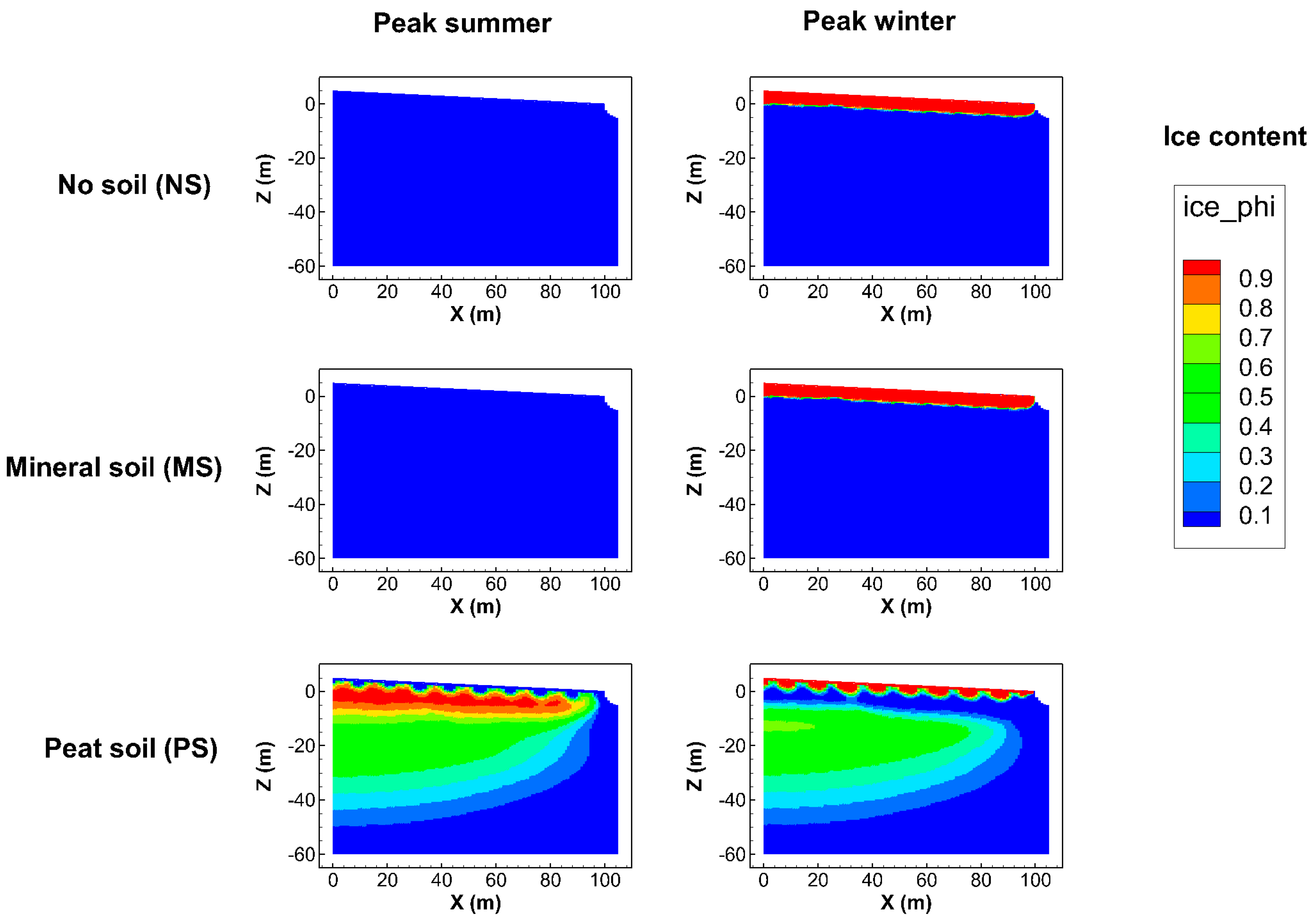
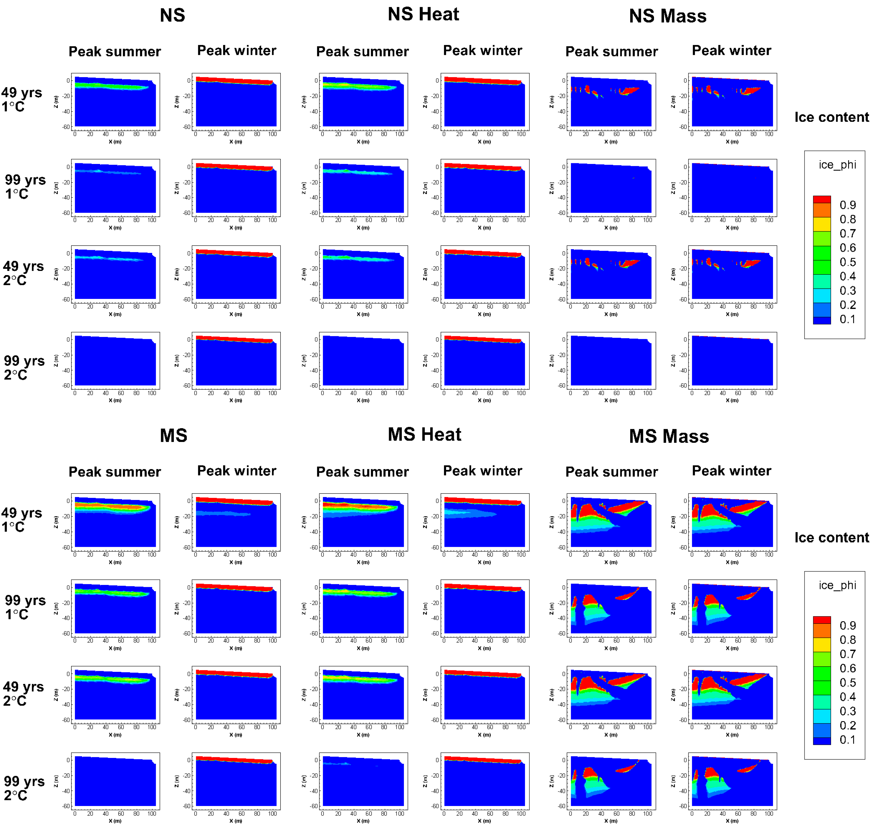
Figure 4 shows the ice content results after 2 °C warming over 100 years (0.02 °C/year);
Figure A2 of the
Appendix shows the corresponding results for the warming trend of 0.01 °C/year. Large differences in subsurface ice content remained after the 2 °C (and the 1 °C) warming (
Figure 4;
Figure A2), as before the warming (
Figure 3). The relatively high ice content still remaining in the PS case after warming is explained by the much greater ice content and depth extent that was there to start with (
Figure 3), along with the higher soil heat capacity and lower soil thermal conductivity compared to the other cases. These properties imply that more heat transport from the surface is needed to increase the subsurface temperature at depth, while this transport by the dominant conduction process is also slower in the PS than in the other cases. Conversely, the relatively small, or zero, ice content remaining after warming in the MS and NS cases is explained by the relatively small ice contents and depth extents that were there to start with (
Figure 3), along with the relatively low soil (or rock for NS) heat capacity and high soil (rock) thermal conductivity in these cases. This property combination implies that less heat transport from the surface is needed to increase the subsurface temperature at depth, while this transport by conduction is also faster in these cases than in the PS case. The lower hydraulic conductivity and porosity in the NS than in the MS case further explain the relatively small difference in remaining ice content after warming between these two cases. Their property differences imply a smaller contribution of waterborne heat advection toward increasing the subsurface temperature and thawing the subsurface ice in the NS than in the MS case.
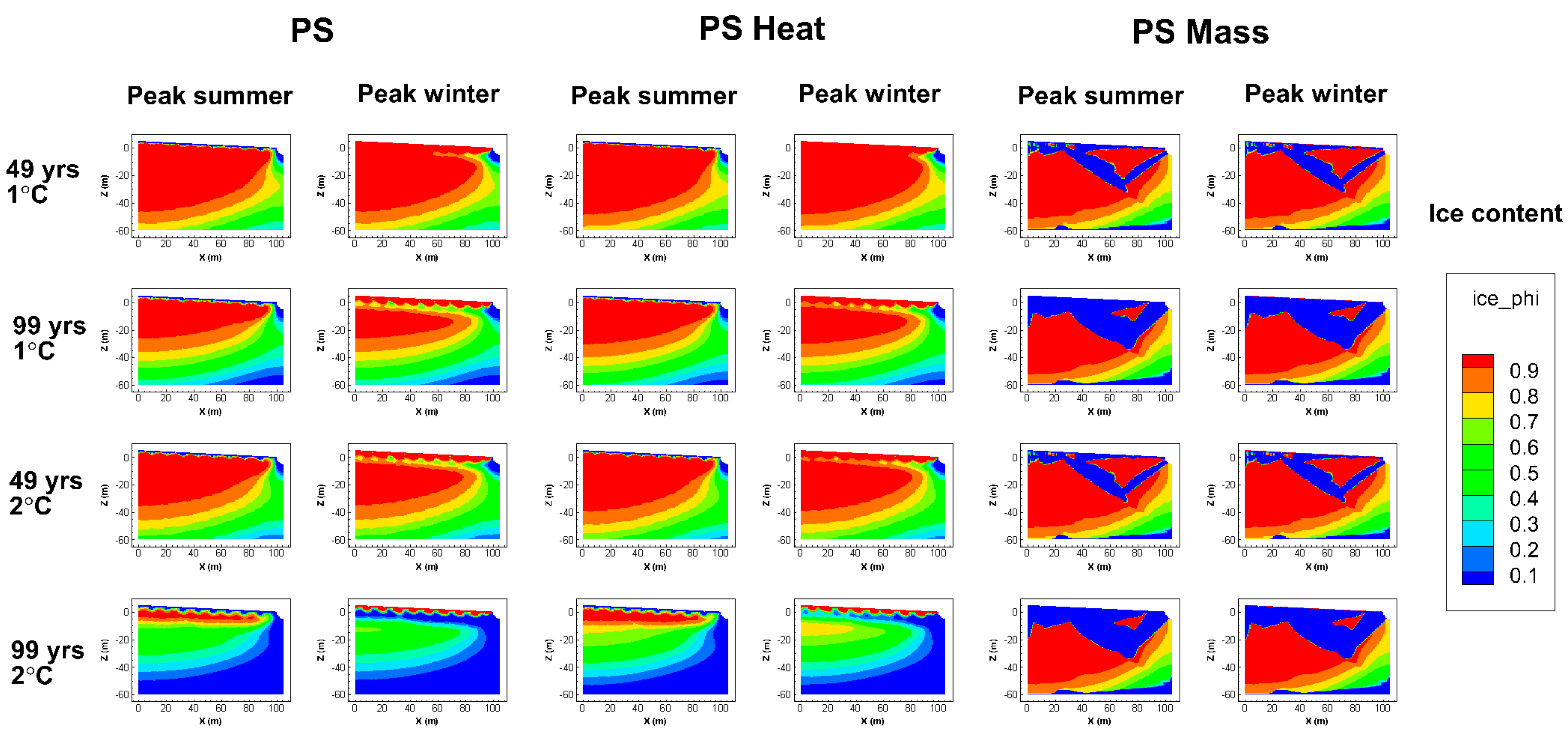
A time lag in the penetration of heat from the surface explain why there is more ice present at the specific time of peak summer than at the time of peak winter in the PS case (
Figure 4 and enlargement of top ten meters in
Figure A3). At peak winter, the top layer is totally frozen, but with a remaining (from summer) unfrozen layer below. As winter progresses from that time, the ice formation moves downwards so that there is still ice present below the surface by the time peak summer arrives, while the ice at the surface is gone due to summer warming until that time. Later during summer, the deeper ice also thaws. When temperatures get colder in the autumn and winter, ice is formed again at the surface. The regular small variations in ice depth near the surface (mostly noticeable in
Figure A3) are numerical effects. Even a minimal disturbance in the numerical solution, amplified by the staircase cell structure in the Cartesian grid that approximates the sloping surface (and sloping layers beneath), initiates some convective heat flow leading to the regular repetitions of small convection cells that are reflected in the small ice depth variations near the surface.
Furthermore, even though the post-warming ice content remains much greater in the PS case than in the MS and NS cases, the PS case also exhibits a greater difference in ice extent between its pre-warming and its post-warming state, which also extends over a much greater depth than in the other cases (
Figure 5). Thus, the same surface warming opens up a greater ice-free subsurface volume at depth in the PS than in the MS and NS cases, through which increased drainage can occur (enhancing the left-hand loop in
Figure 1), and carbon and pathogens can be released and further transported to downgradient surface waters by mobile liquid water. The bedrock below the top soil may not in itself contain much organic material or allow for much waterborne transport. However, commonly occurring fracture zones in the bedrock may both contain such material and convey considerable water flow and material transport; this is why fracture zone occurrence is also considered in the present simulations.
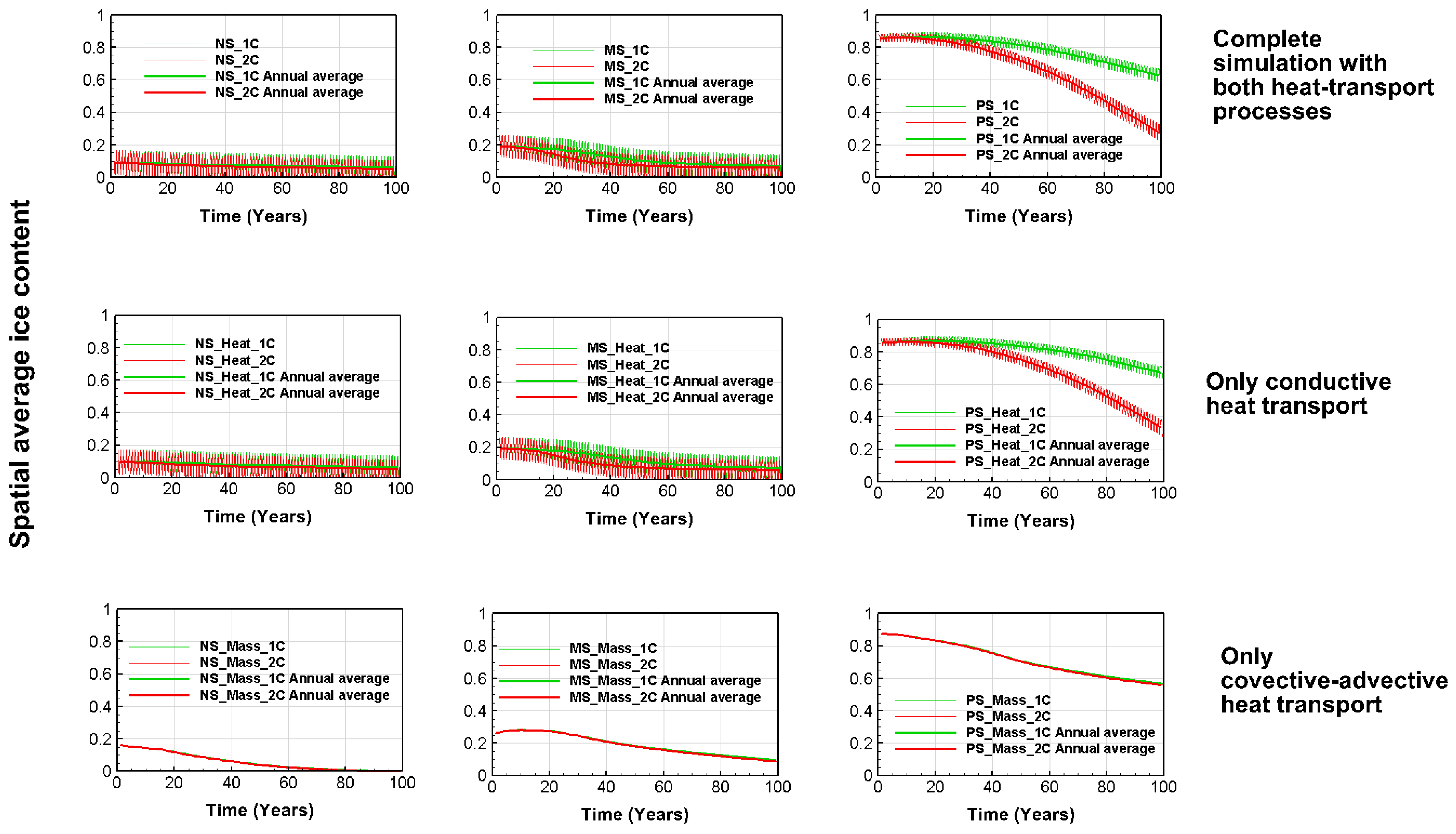
To further test the sensitivity or robustness of these results under different process assumptions, simulations were also performed for only the heat conduction process, or only the heat convection–advection process being active.
Figure 6 shows the resulting evolution over time of ice content averaged over the whole domain and each year;
Figure A4 of the
Appendix shows further results from these simulations. The intra-annual freeze/thaw cycling reflected in short-term fluctuations around the longer-term ice content evolution under warming is only captured if the heat conduction process is active in the simulations. Heat transport by just waterborne convection–advection does not reflect these intra-annual variations, which are smaller relative to annual average ice-content conditions in peatlands than in mineral soils, and largest under no soil conditions. With regard to the long-term evolution of average ice content, the main simulation results are robust, regardless of the considered heat transport process(es) in the simulations. Whether heat is transported from warming at the surface by just conduction, just waterborne convection–advection, or both, the transported heat warms and thaws the subsurface ice such that the resulting average ice content follows a similar overall evolution. This includes relatively small decreases from small initial ice contents and extents over depths in the NS and MS cases, and much greater decrease from much larger initial ice contents and extents over depth in the PS case. In all soil and heat transport cases, the remaining ice content is also similar after 50 years of a 2 °C/100 year warming trend as after 100 years of a 1 °C/100 year warming trend (seen most clearly from
Figure A4 of the
Appendix, by comparing the second and third panel rows for each soil case).
4. Discussion
The presented simulations showed that permafrost formation and thaw, and thereby the associated increase or decrease of thermokarst wetland-lake area in the landscape (
Figure 1), depended strongly on the local soil conditions, and they varied greatly with these for the same large-scale temperature conditions at the land surface. These simulation results are robust and, even though generic, consistent with numerous field findings across the high-latitude permafrost region, as discussed and referred to in the results section [
20,
21,
22,
37,
38]. Specifically, for peatlands (represented by the PS case), the simulations show (as also seen in field observations) much greater ice content and extent over depth than for other soil/rock formations (here, the MS and NS cases), both without and with surface warming trends and regardless of assumptions of dominant heat transport process. In accordance with the field observations cited in the results section, our results are fully consistent with, for example, field reports of permafrost prevailing predominantly in peatlands, and to a much lesser degree in other types of terrain across the southern part of the high-latitude permafrost zone and the lower limit of the mountain permafrost zone [
22,
39]. Moreover, detailed plant macrofossil analysis and radiocarbon dating have shown permafrost occurrence soon after peatland inception and further long-term stability of permafrost in subarctic peat plateaus [
40]. Permafrost mapping in discontinuous permafrost regions has further shown that permafrost distribution is closely related to peatland distribution [
21], with no clear relation found between surface temperature and mean size of frozen landforms or permafrost degradation extent among various peatlands [
20].
The simulations are also robust in revealing that the same surface warming leads to greater subsurface volume thawing at depth in the PS case than in the MS and NS cases. Even though permafrost remains (at a smaller ice-content degree) after warming in the PS case (consistent with the above cited field reports for peatlands), the result of major thawing at depth for peat soils still indicates possible severe consequences of permafrost thaw in such organic soils, as for instance observed in the field with peatlands collapsing into inundated Arctic fens [
23].
As such, our results emphasize greater wetland-related societal and health risks of permafrost thaw in and around peatlands than for other local soil conditions. This assessment also considers that peatlands have among the highest soil organic carbon contents in the northern permafrost region [
38,
41]. The extensive thawing at depth found for peat soil conditions in the present simulations thus indicate possible considerable releases of carbon, various previously frozen pathogens [
8], and DOM, which in turn affects the solar inactivation of pathogens [
14]. Under conditions of thawing permafrost, previous simulation studies have also found the waterborne spreading of organic materials released at depth to the land surface, and its biosphere to be accelerated through activation of new, relatively deep subsurface pathways that were previously frozen or hydrologically isolated by the permafrost [
34].
Consistent with our simulation results and their implications for permafrost thaw in peatlands, a comprehensive review of experimental and observational studies has found permafrost thaw to be one of the main global change impacts on peatlands [
42]. This review also notes that peatland field data are sparse, highly variable, and subject to considerable uncertainties. This highlights the need for process-based model simulation studies, such as the one presented here, for improved understanding, guidance of extended field observations, and scenario analysis of future climate change implications for permafrost thaw dynamics in peatlands, as well as for their thermokarst wetland-lakes and associated societal and health risks.
Cryoturbated mineral soils may also contain high organic carbon contents [
22,
38], for which the present simulation results indicate fast total permafrost degradation under warming. For permafrost thaw at/near the surface, as in the simulated mineral soil case, water infiltration from the surface would increase due to the extended time period within each year with unfrozen, (near-)surface soil, and associated increasing active layer depth. This implies greater groundwater recharge and flow with the potential to carry more thaw-released organic material to downgradient surface waters [
3]. Furthermore, with regard to the debated permafrost protection that may be provided by sand covering (desertification) [
24,
25], the relatively small differences in ice-content results between the simulated MS and NS cases suggest only small such protection effects.
Systematic permafrost simulation studies, like the present one, can improve process-based insights and understanding of similarities, links, and patterns across diverse site-specific data and research findings. The simulation approach used here can also be site-specific and used to guide more detailed and resource-demanding site and regional investigations. The approach can also be adapted to more directly relate to, and provide relevant process-based quantifications for, further site/regional assessments of ecosystems and societal and health risks related to permafrost thaw. Such risks may be closely associated with regime shifts from terrestrial to aquatic wetland ecosystems (right-hand system loop in
Figure 1) or vice versa (left-hand system loop in
Figure 1), with infrastructure failures, DOM and pathogen releases, and feedback to global warming.


