A Novel Approach for Delineation of Homogeneous Rainfall Regions for Water Sensitive Urban Design—A Case Study in Southeast Queensland

Abstract

The delineation of homogeneous regions is primarily based on long-term overall rainfall characteristics and therefore does not necessarily consider the homogeneity of event-based rainfall characteristics. However, event-based rainfall characteristics including antecedent dry days, rainfall intensity, total rainfall and total duration of rainfall events are critical for Water Sensitive Urban Design (WSUD). Accordingly, this study presents a novel approach to objectively identify homogeneous rainfall regions based on event-based rainfall characteristics. This approach uses cluster analysis and Hosking–Wallis heterogeneous tests collectively to test the homogeneity of event-based rainfall characteristics. A case study conducted for southeast Queensland (SEQ), Australia is also presented in this article. This study compares the results of the novel modified approach against results of the conventional approach for the delineation of homogeneous regions. It was evident from the results that the entire SEQ could be treated as a homogeneous rainfall region based on the conventional approach. In contrast, based on the modified approach, the coast and the inland of SEQ were identified as separate homogeneous regions. Further, antecedent dry days and rainfall intensity were recognized as the deciding rainfall characteristics in the delineation of homogeneous rainfall regions.

1. Introduction

The critical features of Water Sensitive Urban Design (WSUD) are estimated by taking historical rainfall records of a representative rainfall station into account. Therefore, selection of an appropriate rainfall station that best represents the characteristics of regional rainfall is important for the design of WSUD. Typically, rainfall stations are selected by identifying potential homogeneous rainfall regions. A homogeneous rainfall region represents a region that has statistically similar rainfall everywhere in the region over a long period of time [1].

There are a range of methods available to identify rainfall homogeneous regions. These methods can be broadly classified into four, namely, geographical convenience, subjective partitioning, objective partitioning and multivariate analysis [1]. Geographical convenience refers to the demarcation of possible homogeneous regions based on administrative boundaries or based on major geographical and physical groupings. This approach is essentially arbitrary and often considered misleading. Subjective partitioning refers to the demarcation of possible homogeneous regions by the inspection of the rainfall characteristics and established prior knowledge about the study area [2]. Objective partitioning involves identifying a group of similar meteorological stations by minimizing a with-in group heterogeneous criterion. Typical heterogeneous criteria used by researchers include with-in group variation of sample coefficients of variation, with-in group variation of sample L-skewness and likelihood-ratio statistics [1,3,4,5]. Multivariate analysis, in particular cluster analysis (CA) and principal component analysis (PCA), are prevalently used across various research studies to group meteorological stations with similar observations [4,6,7,8]. In this regard, a multivariate data matrix that includes critical variables defining the characteristics of the meteorological stations within the study area is used in analysis so that the stations are grouped based on the similarities among them.

Subjective partition approaches are commonly used in identifying the rainfall homogeneous regions in the context of WSUD in Australia. For example, the Brisbane City Council and Moreton Bay Waterways [9] suggest the demarcation of rainfall homogeneous regions for southeast Queensland purely based on the established knowledge of the spatial variation of mean annual rainfall and the number of rain days per year. Similarly, the Northern Territory Department of Planning and Infrastructure [10] recommend single rainfall station data for Darwin, Australia, based on the assumption that the rainfall characteristics across Darwin Region is uniform. There are also instances where the nearest rainfall station has been used to study different aspects of WSUD [11,12,13].

In addition to the inherent subjectiveness in the existing approach, there are also those based on overall rainfall characteristics such as average annual rainfall, average number of wet days per year or average number of dry days per year [9]. However, the delineation of homogeneous rainfall region based on these variables may be misleading for WSUD [11,13]. In the context of WSUD, event-based rainfall characteristics are perceived with more importance than the overall rainfall characteristics. Rainfall event characteristics such as antecedent dry days, rainfall intensity, total rainfall and rainfall duration are critical characteristics of rainfall that are directly related to the stormwater quality and quantity. Stormwater quantity is directly linked to the total rainfall depth, duration and rainfall intensities [13,14,15,16,17]. Stormwater quality is primarily influenced by the pollutant processes, namely, build-up and wash-off. Build up is primarily a function of antecedent dry days [18], and wash-off is a function of rainfall intensity [18,19]. In addition, concentrations of different pollutants are found to be associated with different rainfall characteristics. For example, Wang et al. [20] found that the nitrogen concentration in stormwater runoff is inversely proportional to the rainfall duration. Lee and Bang [21] suggested that the concentration of suspended solids and chemical oxygen demand (COD) are proportional to the rainfall durations. In addition, in the context of climate change, the event-based rainfall characteristics are expected to change in most parts of the world while the average rainfall conditions remain more or less the same.

Therefore, it is critical to incorporate event-based rainfall characteristics in defining the homogeneous regions and thereby selecting the representative rainfall station for the design of WSUD. This paper presents a novel approach to objectively demarcate the rainfall homogeneous regions based on event-based rainfall characteristics.

2. Materials and Methods

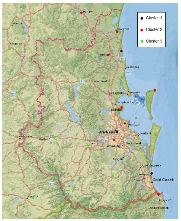
2.1. Study Area

Southeast Queensland was selected as the study area. Southeast Queensland has an extensive meteorological station network with measurements taken in daily, 3 h, 30 min and 1 min (pluviography) formats. For this study, pluviographic rainfall data for 17 stations were collected from the Weather Station Directory of the Bureau of Meteorology (BoM), Australia, for the period between 2011 and 2015 primarily based on the availability of data. The stations used for this analysis and their geographical information are presented in

Table 1. Summary of the selected meteorological stations for analysis.

Serial No.	Station No.	Station	Latitude	Longitude	No. of Events (2011–2015)
1	40004	Amberley AMO	−27.6297	152.7111	265
2	40043	Cape Moreton Lighthouse	−27.0314	153.4661	350
3	40082	University of Queensland	−27.5436	152.3375	274
4	40093	Gympie	−26.1831	152.6414	379
5	40211	Archerfield Airport	−27.5717	153.0078	358
6	40717	Coolangatta	−28.1681	153.5053	501
7	40764	Gold Coast Seaway	−27.939	153.4283	455
8	40842	Brisbane Aero	−27.3917	153.1292	377
9	40861	Sunshine Coast Airport	−26.6006	153.0903	471
10	40908	Tewantin RSL Park	−26.3911	153.0403	426
11	40913	Brisbane	−27.4808	153.0389	380
12	40922	Kingaroy Airport	−26.5737	151.8398	249
c	40958	Redcliffe	−27.2169	153.0922	385
14	40983	Beaudesert Drumley St	−27.9707	152.9898	297
15	40988	Nambour Daff—Hillside	−26.6442	152.9383	506
16	41525	Warwick	−28.2061	152.1003	213
17	41529	Toowoomba Airport	−27.5425	151.9134	275

.

2.2. Event Seperation

Individual events were separated, and variables such as antecedent dry days, maximum rainfall intensity, total rainfall depth and the rainfall duration of each event were determined. These event-based rainfall characteristics are critical rainfall characteristics that influence stormwater quality and quantity. For example, pollutant build-up is primarily influenced by the antecedent dry days [11,13,14,15], while the pollutant wash-off is influenced by the rainfall intensity [11,13] or total rainfall depth [22], which are the two processes that ultimately determine the stormwater quality. In addition, the total rainfall depth and duration of a rainfall event are directly related to the quantity of stormwater generated from a catchment [13,17]. Therefore, a demarcation of homogeneous regions based on the event-based rainfall characteristics such as antecedent dry days, rainfall intensity, total rainfall depth and rainfall duration is more appropriate.

The following criteria were considered in separating individual rainfall events:

• An event was considered independent only if the consecutive event was separated by at least 3 h antecedent duration. Otherwise, those events were treated as a single event. There is no guideline or literature available to suggest an accurate value for minimum antecedent dry period to consider two consecutive events as independent events. Therefore, 3 h was selected as a reasonable value based on previous experience and expert advice.
• An event that constituted less than 1 mm total rainfall for a period greater than 1 h was not considered as a storm event and not considered for the analysis.
• The maximum rainfall intensity (in mm/h) of the events was estimated by calculating the moving total of 1 h rainfall throughout the rainfall duration.
• Any event having data entries of false quality based on quality classifications of BoM was discarded from the study.

2.3. Cluster Analysis

A cluster can be referred to as the formed group of objects with similar attributes in which the objects within the particular clusters are more relatable to each other and are clearly different from any objects from a different cluster. The higher the closeness of objects within the cluster and the higher the difference between different clusters will make the cluster analysis sound and accurate.

Many studies have opted for cluster analysis in identifying homogeneous rainfall regions, e.g., Terassi et al. [23], Lyra et al. [24], Goyal et al. [25] and Oliveira-Junior et al. [26]. However, the approaches and the algorithms used to perform the cluster analysis are inherently different. Among the commonly used cluster analyses, k-means clustering and hierarchical clustering are the most predominantly used clustering approaches [27].

2.3.1. k-Means Clustering

The number of clusters in k-mean clustering is user-defined and referred to as k. Once the k is defined, k number of random centroids are selected, and each object is assigned to the closest centroids to form clusters. The closest centroid is assigned based on the smallest Euclidean distance to the centroids as given by:

$$dist\left(x,c\right)=\sqrt{{{\displaystyle \sum }}_{i=1}^n{\left(x_i-c_i\right)}^2},$$

(1)

where $x=\left(x_1, x_2,x_3,\dots ,x_n\right)$ and $c=\left(c_1, c_2,c_3,\dots ,c_n\right)$ denote the objects and the centroids of the clusters, and $dist\left(x,c\right)$ denotes the Euclidean distance between x and c. Then, the centroids of the clusters are again calculated and used as the new centroids. The objects are then assigned to the closest new centroids. This process is repeated until the centroids remain unchanged.

The quality of the k-means clustering can be expressed by an objective function that can be determined by the proximities of the objects to the cluster centroids. The Sum of Square Error (SSE), also referred to as scatter, is the most common index used to measure the quality of the clustering. SSE calculates the Euclidian distance of each object to their closest centroids, and the computation of SSE can be given by:

$$\mathrm{SSE}={{\displaystyle \sum }}_{i=1}^k{{\displaystyle \sum }}_{xϵc_i}dist{\left(c_i, x\right)}^2,$$

(2)

where c denotes the centroids and x denotes the objects assigned to that particular centroid.

2.3.2. Hierarchical Clustering

Hierarchical clustering initially considers every single object as an individual cluster and successively merges the closest next cluster based on the Euclidean distance, as given in Equation (1), until they form a single cluster. This formation is typically presented in a dendrogram, which displays all sub-clusters and the order in which they merge. The proximity among the clusters is defined by three different approaches, namely, simple link, complete link and group average. Single link defines the proximities of the clusters based on the Euclidean distance between the closest two points of different clusters while the complete link defines the proximities based on the farthest points of different clusters. The group average determines the average pairwise Euclidean distance (for all objects) to measure the proximity of clusters.

2.4. Hosking–Wallis Heterogeneity Test

The Hosking–Wallis heterogeneity test is commonly applied for identifying the homogeneous rainfall regions in regional rainfall frequency analysis [28,29,30]. The Hosking–Wallis heterogeneity test has been opted into this research to objectively test the rainfall homogeneity of a region. This test primarily compares the variations in the L-moment ratios between the meteorological stations of the actual regions and a set of artificially created homogeneous regions (based on the average rainfall characteristics of the region).

In an ideal situation, every station in a homogeneous region should have the same L-moment ratios. However, in practice, the L-moments ratio are different for every meteorological station due to differences in their observations. Nevertheless, they can be reasonably treated as homogeneous if the differences in the L-moment ratios of the meteorological stations are statistically insignificant [1].

Accordingly, the Hosking–Wallis heterogeneity test estimates the degree of heterogeneity of a group of meteorological stations using a set of statistical indexes called H indexes. H indexes compare the between-station dispersion of L-moment ratios for a group of stations with what would be expected for an artificially developed homogeneous region. The artificial homogeneous region is developed by repeated simulations that generate synthetic rainfall data with the same record lengths of the actual meteorological stations based on the regional average L-moments. The regional weighted average of L-CV—t^(R), L-skewness—t₃^(R), and L-kurtosis—t₄^(R) in the Hosking–Wallis heterogeneity test are calculated as:

$$t^R=\frac{{{\displaystyle \sum }}_{j=1}^N{n}_j{t}^j}{{{\displaystyle \sum }}_{j=1}^N{n}_j},$$

(3)

$$t_3{}^R=\frac{{{\displaystyle \sum }}_{j=1}^N{n}_j{t}_3{}^j}{{{\displaystyle \sum }}_{j=1}^N{n}_j},$$

(4)

$$t_4{}^R=\frac{{{\displaystyle \sum }}_{j=1}^N{n}_j{t}_4{}^j}{{{\displaystyle \sum }}_{j=1}^N{n}_j},$$

(5)

where N denotes the number of stations in the region and n_j denotes the record length of station j.

In order to measure the heterogeneity of the meteorological stations, the Hosking–Wallis heterogeneity test suggests three dispersion measures, namely, V₁, V₂ and V₃ based on the L-coefficient of variation, L-coefficient of variation and L-skewness and L-skewness and L-kurtosis, respectively, as given by:

$$V_1={\left\{\frac{{{\displaystyle \sum }}_{j=1}^n{n}_j{\left(t^j-t^R\right)}^2}{{{\displaystyle \sum }}_{j=1}^n{n}_j}\right\}}^{1/2},$$

(6)

$$V_2=\frac{{{\displaystyle \sum }}_{j=1}^n{n}_j {\{{\left(t^j-t^R\right)}^2+{\left(t_3{}^j-t_3{}^R\right)}^2\}}^{1/2} }{{{\displaystyle \sum }}_{j=1}^n{n}_j},$$

(7)

$$V_3=\frac{{{\displaystyle \sum }}_{j=1}^n{n}_j {\left\{{\left(t_3{}^j-t_3{}^R\right)}^2+{\left(t_4{}^j-t_4{}^R\right)}^2\right\}}^{1/2} }{{{\displaystyle \sum }}_{j=1}^n{n}_j} .$$

(8)

In order to simulate the dispersion measurements for the artificial homogeneous region, a four-parameter kappa distribution is fitted to the regional average L-moment ratios (1, t^R, t₃^R and t₄^R) to simulate N_sim realizations of artificial homogeneous regions (with the same record lengths of the actual meteorological stations). The mean μ_v and the standard deviation σ_v of the dispersion measurements of the artificially simulated homogeneous region are calculated. Then, the dispersions of the actual and simulated homogeneous regions are compared using the statistical index H_i (for i = 1, 2 and 3) as given by:

$$H_i=\frac{\left(V_i-{\mathsf{\mu }}_v\right)}{{\sigma }_v} .$$

(9)

Accordingly, three statistical indexes, H₁, H₂ and H₃, are calculated based on the corresponding dispersion measures V₁, V₂ and V₃. The region is declared acceptably homogeneous if H_i < 1, possibly heterogeneous if 1 ≤ H_i < 2 and definitely heterogeneous if H_i ≥ 2 [1].

Furthermore, Hosking et al. [1] suggested that dispersion index H₁ alone can be used to identify homogeneous regions as it has higher discriminatory power than other indexes. However, many studies use all three dispersion indexes or at least the first two dispersion indexes to identify homogeneous regions [31,32]. Therefore, in this study, only the first two indexes, H₁ and H₂, have been used to assess the degree of homogeneity of the region. The dispersion indexes were generated using an R package named ‘homtests’ [32].

3. Results and Discussion

The delineation of homogeneous regions in southeast Queensland was carried out using the conventional approach and the modified approach specifically designed to suit the requirements for WSUD, considering event-based rainfall characteristics.

3.1. Conventional Approach

In the conventional approach, the rainfall data of a set of the selected meteorological stations are tested for homogeneity purely based on the probabilistic characteristics of the continuous rainfall records. The method does not necessarily consider probabilistic characteristics of individual rainfall events.

Firstly, we performed the Hosking–Wallis heterogeneous test for the selected 17 stations in SEQ. The statistical indexes of heterogeneity, H₁ and H₂, were calculated for 500 simulations of realizations using the R-package ‘homtests’ [32]. The results suggested that the entire region could be treated as homogeneous, with H₁ = 0.6483 and H₂ = 0.9142. The codes executed to run the package are provided in Appendix A.

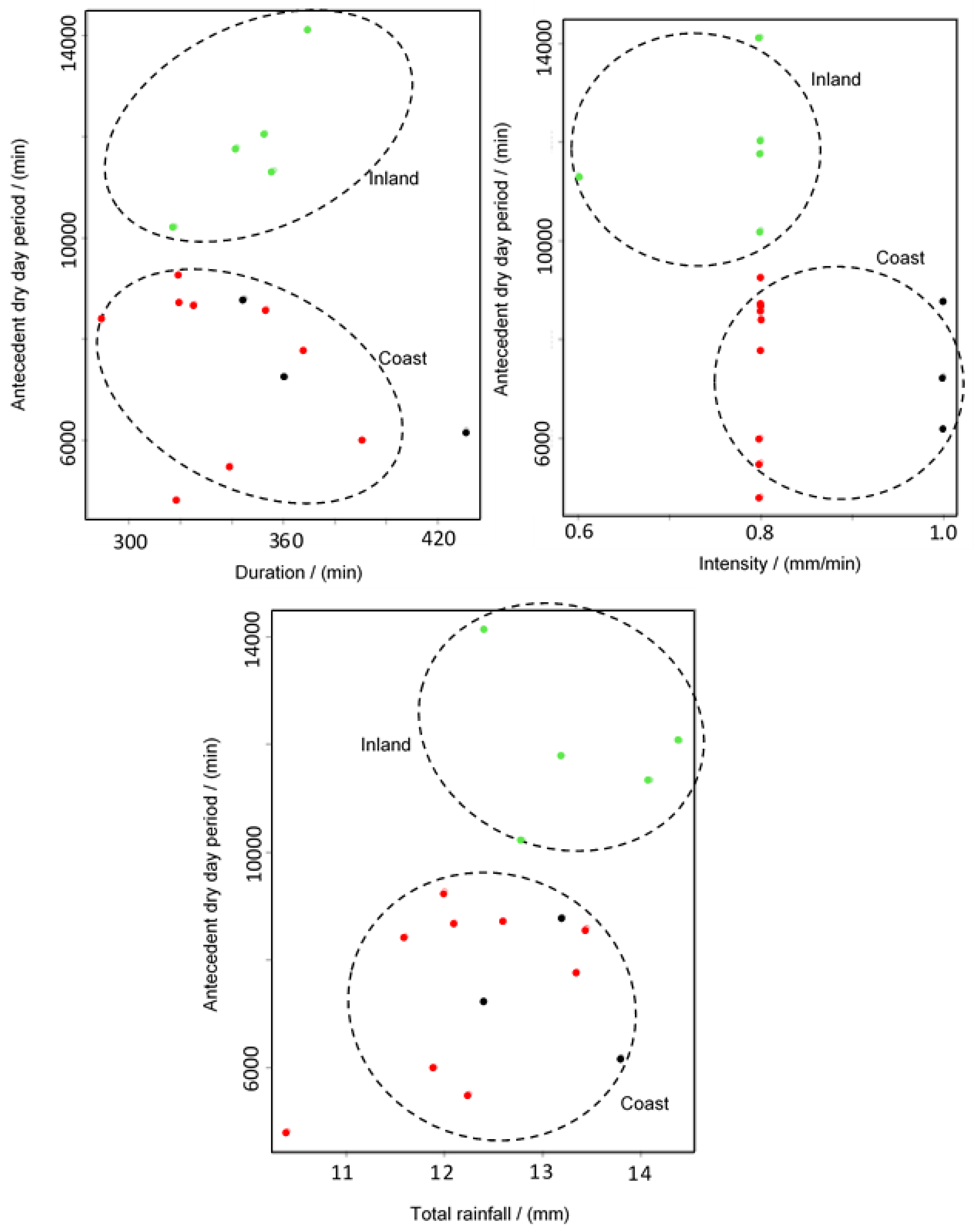
3.2. Modified Approach

Although the overall rainfall characteristics of the entire SEQ were homogeneous, the event-based rainfall characteristics of the region may be different. For example, an event with intense rainfall for a short period of time and an event with less intense rainfall for a longer period of time may result in similar overall (average) rainfall characteristics. However, these events can potentially produce completely different stormwater quality and quantity scenarios. Therefore, it was important to consider the homogeneity of rainfall stations based on event-based rainfall characteristic when selecting the representative meteorological stations for WSUD.

Table 2. Heterogeneous index for southeast Queensland. Results based on the current approach.

Event Characteristics	${\mathit{H}}_1$	${\mathit{H}}_2$	Remarks
Antecedent dry days	3.37	1.16	Heterogeneous
Maximum rainfall intensity	1.95	0.59	Possibly heterogeneous
Total rainfall	0.81	0.32	Homogeneous
Duration	0.25	0.10	Homogeneous

presents the outcomes of the Hosking–Wallis heterogeneity tests performed for individual rainfall characteristics. The results suggest that the study area was potentially heterogeneous based on the H₁ and H₂ values.

Based on the first two dispersion indexes (H₁ and H₂), antecedent dry day showed a higher level of heterogeneity compared to other event-based rainfall characteristics. The maximum rainfall was found to be potentially heterogeneous across SEQ. In contrast, total rainfall and rainfall duration were homogeneous across SEQ. Overall these results suggest that the entire SEQ cannot be considered homogeneous based on all event-based rainfall characteristics. Accordingly, homogeneous regions suggested based on the continuous-rainfall approach may not necessarily be homogeneous based on individual rainfall characteristics. In addition, it was also noticeable that the antecedent dry days and the maximum rainfall intensity showed heterogeneity among the rainfall stations while the total duration and the total rainfall of the events were homogeneous. Therefore, it can be concluded that antecedent dry day periods and maximum rainfall intensity have higher spatial variation and thus should be the deciding rainfall characteristics in the delineation of homogeneous regions.

Accordingly, the next step was to identify all potential homogeneous regions inside SEQ and to assess the degree of homogeneity of the identified potential homogeneous regions (using the Hosking–Wallis heterogeneity test). This step was performed using cluster analysis. Agglomerative hierarchical cluster analysis and k-means cluster analysis were performed using R package ‘stats’ [33]. The parameters used for the analysis included 3rd quartile (Q3) values of antecedent dry days, maximum rainfall intensity, total rainfall and duration of the individual events of each station as given in

Table 3. Third quartile values of antecedent dry days, maximum rainfall intensity, total rainfall and rainfall duration of the selected 17 stations in southeast Queensland.

Serial No.	Station No.	3rd Quartile Values—Q3
		Antecedent Dry Day/(days)	Maximum Intensity/(mm/h)	Total Rainfall/(mm)	Duration (h)
1	40004	6.4	7.1	12.0	5.3
2	40043	5.4	6.7	13.4	6.1
3	40082	8.4	7.6	14.4	5.9
4	40093	6.0	6.0	13.5	5.9
5	40211	5.9	6.8	11.6	4.8
6	40717	3.8	6.4	12.3	5.7
7	40764	5.0	7.0	12.4	6.0
8	40842	6.0	6.6	12.1	5.4
9	40861	4.3	8.2	13.8	7.2
10	40908	3.3	5.9	10.4	5.3
11	40913	6.1	7.4	13.2	5.8
12	40922	9.8	8.2	12.4	6.2
13	40958	6.1	7.3	12.6	5.3
14	40983	7.1	7.6	12.8	5.3
15	40988	4.2	6.2	11.9	6.5
16	41525	7.9	6.6	14.1	5.9
17	41529	8.2	7.8	13.2	5.7

. This was because the average or the median of the rainfall characteristics at the meteorological stations considered were expected to be similar in nature and therefore may not be grouped into discrete clusters. In contrast, selecting a higher quartile value may result in too many unrealistic clusters. Our repeated analysis suggested that the use of the 3rd quartile values provide the most appropriate outcomes. The analysis suggested three potential clusters based on the dendrogram shown in Figure 1. Accordingly, Cluster 1 comprised Stations 9, 7 and 11. Cluster 2 comprised Stations 3, 12, 14, 16 and 17 and Cluster 3 comprised Stations 1, 5, 6, 8, 10, 13 and 15. However, the geographical locations of the meteorological stations of the clusters as presented in Figure 2 suggested that the meteorological stations of Cluster 1 and Cluster 2 were located in close proximity to the SEQ coast and the meteorological stations of Cluster 3 were located inland. Furthermore, Cluster 1 and Cluster 2 stations did not show a clear geographical separation.

Furthermore, scatter plots produced to examine the meteorological stations of the three clusters based on the considered rainfall characteristics are presented in Figure 3. It can be observed from Figure 3 that the rainfall stations of Cluster 3 have clear distinctions between the rainfall stations of Cluster 1 and Cluster 2. In contrast, the rainfall station of Cluster 1 and Cluster 2 showed no clear separations. These results suggest that Cluster 1 and Cluster 2 can be treated as single clusters representing coastal SEQ while Cluster 3 represents inland SEQ. Accordingly, two potential homogeneous regions were identified within the study area, namely, Coastal-SEQ and Inland-SEQ.

The degree of homogeneity of the identified regions of Coastal-SEQ and Inland-SEQ were evaluated by performing the Hosking–Wallis heterogeneity tests using event-based rainfall characteristics. The summary of the results is presented in

Table 4. Dispersion indexes for Hosking–Wallis heterogeneity test for Coastal-southeast Queensland (SEQ) and Inland-SEQ.

Event Characteristics	Coastal-SEQ		Inland-SEQ
	H1	H2	H1	H2
Antecedent dry day periods	−0.20	1.18	−0.35	0.06
Maximum rainfall intensity	0.78	0.97	−0.61	−0.65
Total rainfall	−0.55	0.65	−0.54	−0.10
Duration	0.26	0.32	−1.29	−1.00

. As shown in Table 4, the dispersion indexes H₁ and H₂ were found to be less than one for all the rainfall characteristics for both Coastal-SEQ and Inland-SEQ. Therefore, Coastal-SEQ and Inland-SEQ were identified as two separate homogeneous regions within SEQ based on the event-based rainfall characteristics.

4. Conclusions

The entire southeast Queensland can be treated as a homogeneous region based on the conventional (continuous-rainfall) approach. However, based on individual rainfall characteristics such as antecedent dry days, maximum rainfall intensity, total rainfall and duration of the rainfall events, there were two separate homogeneous regions identified.

This implies that although the characteristics of the continuous rainfall data between stations were statistically similar, the event-based characteristics can have significant differences among stations. Therefore, the conventional approach in delineating rainfall homogeneous regions may be misleading in the context of Water Sensitive Urban Design. The newly proposed approach in this study is technically more robust and provides reliable results.

The outcomes of this study can also be broadly related in any rainfall homogeneous assessment. The most common use of homogeneous testing is regional frequency estimations. Many of the regional frequency analyses are based on the conventional Hosking and Wallis [1] regionalization approach including the revised Intensity-Frequency-Duration (IFD) estimates for Australia [34], where stations were grouped with the assumption that all the stations in the homogeneous regions have a similar probability distribution with a single scaling factor. However, as discussed, the current approach does not check the homogeneity based on individual rainfall characteristics. Therefore, the method adopted in this study can be effectively used in identifying homogeneous regions in the regional frequency analysis especially for studies that depend on the event-based characteristics of rainfall such as Water Sensitive Urban Design.

The newly proposed approach for identifying homogeneous rainfall region is more suitable in studies related to climate change. This is because the common outcomes from studies related to future rainfall trends suggest that although not many changes are expected in the overall rainfall characteristics, the rainfall patterns and characteristics are expected to change significantly in the future. Therefore, it will be more appropriate to apply the approach presented in this study in defining the rainfall homogeneous regions in the context of climate change.

References

1. Hosking, J.; Wallis, J. Regional Frequency Analysis: An Approach Based on L-Moments; Cambridge University Press: Cambridge, UK, 1997. [Google Scholar]
2. Schaefer, M.G. Regional analyses of precipitation annual maxima in Washington State. Water Resour. Res. 1990, 26, 119–131. [Google Scholar] [CrossRef]
3. Pearson, C.P. New Zealand regional flood frequency analysis using L-moments. J. Hydrol. 1991, 30, 53–64. [Google Scholar]
4. Lin, G.F.; Chen, L.H. Identification of homogeneous regions for regional frequency analysis using the self-organizing map. J. Hydrol. 2006, 324, 1–9. [Google Scholar] [CrossRef]
5. Ngongondo, C.S.; Xu, C.Y.; Tallaksen, L.M.; Alemaw, B.; Chirwa, T. Regional frequency analysis of rainfall extremes in Southern Malawi using the index rainfall and L-moments approaches. Stoch. Environ. Res. Risk Assess. 2011, 25, 939–955. [Google Scholar] [CrossRef] [Green Version]
6. Munoz-Diaz, D.; Rodrigo, F.S. Spatio-temporal patterns of seasonal rainfall in Spain (1912–2000) using cluster and principal component analysis: comparison. Ann. Geophys. 2004, 22, 1435–1448. [Google Scholar] [CrossRef]
7. Unal, Y.; Kindap, T.; Karaca, M. Redefining Climate Zones for Turkey Using Cluster Analysis. J. Hydrol. 2003, 23, 1045–1055. [Google Scholar] [CrossRef]
8. Dyer, T.G. The assignment of Rainfall stations into homogeneous groups: An application of principal component analysis. Q. J. R. Meteorol. Soc. 1975, 101, 1005–1013. [Google Scholar] [CrossRef]
9. BCC MBW. Water Sensitive Urban Design Technical Design Guidelines for South East Queensland; South East Queensland Healthy Waterways Partnership and Brisbane City Council: Brisbane, Australia, 2006; Volume 1.
10. NDTPI. Water Sensitive Urban Design Planing Guide—Final; Northern Territory Department of Planning and Infrastructure: Darwin Australia, 2009.
11. Liu, A. Influence of Rainfall and Catchment Characteristics on Urban Stormwater Quality. Ph.D. Thesis, Faculty of Built Environment and Engineering, Queensland University of Technology, Brisbane, Australia, 2011. [Google Scholar]
12. Ma, Y. Human Health Risk of Toxic Chemical Pollutants Generated from Traffic and Land Use Activities. Ph.D. Thesis, Queensland University of Technology, Brisbane, Australia, 2016. [Google Scholar]
13. Egodawatta, P. Translation of Small Plot Pollution Mobilisation and Transport Measurement from Impermeable Urban Surface to Urban Catchment Scale. Ph.D. Thesis, Faculty of Built Environment and Engineering, Queensland University of Technology, Brisbane, Australia, 2007. [Google Scholar]
14. Luo, P.; Mu, D.; Xue, H.; Ngo-Duc, T.; Dang-Dinh, K.; Takara, K.; Nover, D.; Schladow, G. Flood inundation assessment for the Hanoi Central Area, Vietnam under historical and extreme rainfall conditions. Sci. Rep. 2018, 8, 12623. [Google Scholar] [CrossRef]
15. Luo, P.; He, B.; Duan, W.; Takara, K.; Nover, D. Impact assessment of rainfall scenarios and land-use change on hydrologic response using synthetic Area IDF curves. J. Flood Risk Manag. 2018, 11, S84–S97. [Google Scholar] [CrossRef]
16. Luo, P.; He, B.; Takara, K.; Xiong, Y.E.; Nover, D.; Duan, W.; Fukushi, K. Historical Assessment of Chinese and Japanese Flood Management Policies and Implications for Managing Future Floods. Environ. Sci. Policy 2015, 48, 265–277. [Google Scholar] [CrossRef]
17. Zoppou, C. Review of urban storm water models. Environ. Model. Softw. 2001, 16, 195–231. [Google Scholar] [CrossRef]
18. Sartor, J.D.; Boyd, G.B.; Agardy, F.J. Water Pollution Aspects of Street Surface Contaminants. J. Water Pollut. Control Fed. 1974, 46, 458–467. [Google Scholar] [PubMed]
19. Ball, J.E.; Jenks, R.; Aubourg, D. An assessment of the availability of pollutant constituents on road surfaces. Sci. Total Environ. 1998, 209, 243–254. [Google Scholar] [CrossRef]
20. Wang, W.P.; Zhang, P.P.; Ye, X.Q. Study on Rainfall and Roof Rainwater Quality Changes Oriented to Stormwater Recycling. In Proceedings of the 2010 4th International Conference on Bioinformatics and Biomedical Engineering, Chengdu, China, 10–12 June 2010. [Google Scholar]
21. Lee, J.H.; Bang, K.W. Characterization of urban stormwater runoff. Water Res. 2000, 34, 1773–1780. [Google Scholar] [CrossRef]
22. Chiew, F.H.S.; McMahon, T.A. Modelling runoff and diffuse pollution loads in urban areas. Water Sci. Technol. 1999, 39, 241–248. [Google Scholar] [CrossRef]
23. Terassi, P.; Galvani, E. Identification of Homogeneous Rainfall Regions in the Eastern Watersheds of the State of Paraná, Brazil. Climate 2017, 5, 53. [Google Scholar] [CrossRef]
24. Lyra, G.B.; Oliveira-Júnior, J.F.; Zeri, M. Cluster analysis applied to the spatial and temporal variability of monthly rainfall in Alagoas state, Northeast of Brazil. Int. J. Climatol. 2014, 34, 3546–3558. [Google Scholar] [CrossRef]
25. Goyal, M.K.; Gupta, V. Identification of Homogeneous Rainfall Regimes in Northeast Region of India using Fuzzy Cluster Analysis. Water Res. Manag. 2014, 28, 4491–4511. [Google Scholar] [CrossRef]
26. de Oliveira-Júnior, J.F.; Xavier, F.M.G.; Teodoro, P.E.; de Gois, G.; Delgado, R.C. Cluster analysis identified rainfall homogeneous regions in Tocantins state, Brazil. Biosci. J. 2017, 33. [Google Scholar] [CrossRef]
27. Tan, P.N.; Steinbach, M.; Kumar, V. Cluster Analysis: Basic Concepts and Algorithms. Introd. Data Min. 2006, 8, 487–568. [Google Scholar]
28. Fowler, H.J.; Kilsby, C.G. A regional frequency analysis of United Kingdom extreme rainfall from 1961 to 2000. Int. J. Climatol. 2003, 23, 1313–1334. [Google Scholar] [CrossRef] [Green Version]
29. Trefry, C.M.; Watkins, D.W., Jr.; Johnson, D. Regional Rainfall Frequency Analysis for the State of Michigan. J. Hydrol. Eng. 2005, 10, 437–449. [Google Scholar] [CrossRef]
30. Raes, D. Frequency analysis of rainfall data. In KU Leuven and Inter-University Programme in Water Resources Engineering (IUPWARE); KU Leuven: Leuven, Belgium, 2004. [Google Scholar]
31. Kumar Mishra, B.; Herath, S. Assessment of Future Floods in the Bagmati River Basin of Nepal Using Bias-Corrected Daily GCM Precipitation Data. J. Hydrol. Eng. 2015, 20, 05014027. [Google Scholar] [CrossRef]
32. Viglione, A. homtest: Homogeneity Tests for Regional Frequency Analysis; R Foundation for Statistical Computing: Vienna, Austria, 2012. [Google Scholar]
33. R Development Core Team. R: A Language and Environment for Statistical Computing; R Foundation for Statistical Computing: Vienna, Austria, 2016. [Google Scholar]
34. Green, J.; Xuereb, K.; Johnson, F.; Moore, G. The Revised Intensity-Frequency-Duration (IFD) Design Rainfall Estimates for Australia—An Overview; Engineers Australia: Barton, Australia, 2012. [Google Scholar]
Figure 1. Dendrogram of the cluster analysis.
Water 11 00570 g001
Figure 2. Geographical locations of the rainfall stations.
Water 11 00570 g002
Figure 3. Scatter plots of the identified three clusters. Black dots: Cluster 1; red dots: Cluster 2; green dots: Cluster 3.
Water 11 00570 g003