Dynamics of the Flow Exchanges between Matrix and Conduits in Karstified Watersheds at Multiple Temporal Scales


1
Géosciences Environnement Toulouse (UMR 5563 CNRS UPS IRD CNES), Université de Toulouse, 31400 Toulouse, France
2
UMR 1114 EMMAH, INRA-Avignon Université, 84916 Avignon, France
3
Normandie Université, UNIROUEN, UINCAEN, CNRS, M2C, 76000 Rouen, France
4
HydroSciences Montpellier (HSM), Université de Montpellier, CNRS, IRD, 34090 Montpellier, France
*
Author to whom correspondence should be addressed.
Water 2019, 11(3), 569; https://doi.org/10.3390/w11030569
Submission received: 22 February 2019
/
Revised: 12 March 2019
/
Accepted: 15 March 2019
/
Published: 19 March 2019
(This article belongs to the Special Issue Hydraulic Behavior of Karst Aquifers)
Abstract
:The focus of this paper is to investigate the ability to assess the flow exchanges between the matrix and the conduits in two karstified watersheds (Aliou and Baget, Ariège, France) using the KarstMod modeling platform. The modeling is applied using hourly and daily time series. First, the flow dynamics between the conduit and the surrounding matrix are described on a rainfall event scale (i.e., a few days). The model allows us to describe a physical reality concerning the flow reversal between matrix and conduit when there is a significant rainfall event. Then, the long-term trends (i.e., inter-annual) in the matrix water level are evidenced using the moving average over shifting horizon method (MASH). The mean water level in the matrix dropped about 10% to 15% since the late 1960s. Also, the matrix recharge has been delayed from February in the late 1960s to April since the 1990s. Moreover, the contribution of the matrix in the total spring flow is estimated though mass balance. It is estimated that the annual matrix contribution in the total spring flow is about 3% and it can increase to up to 25% during periods with low rainfall.
1. Introduction
Carbonate watersheds throughout the world are very often characterized by karst features. Karstification processes occur when the following conditions are met: (1) mechanical actions create fissures and fractures; (2) water-dissolved CO2 reacts with carbonate rock and (3) hydraulic gradient is sufficiently high to ensure the water renewal and to maintain the karstification potential [1]. This results in complex structures with a heterogeneous permeability field and non-linear hydraulic behavior. Drainage in karstic systems consists of an underground self-organized structure leading to preferential water pathways through a conduit network embedded in either a porous matrix which sometimes is highly permeable (i.e., Floridan Karst aquifer) or a low permeable fissured matrix [2,3]. This drainage organization might be divided between (1) a ‘main drainage system’ (MDS), associated to rapid transit time and (2) an ‘annexe drainage system’ (ADS), associated with a long period of water residence [4,5]. As a result, groundwater water flow in the karstic system could be divided into several compartments with contrasted hydrodynamic behavior.
Four compartments are classically distinguished in karstic aquifers: (1) The impluvium consists of the recharge area composed of either karstic or non-karstic formations, or any combinations of those formations [5]. (2) The epikarst constitutes the uppermost zone with a relatively homogeneous hydraulic conductivity field at the top and becomes heterogeneous in its bottom, leading to a flow concentration towards deeply drainage structures [3,6]. (3) The transmission zone consists of a non-saturated zone between the epikarst and the deeper saturated-zone. In some systems, this compartment can play an important role in the overall hydrological dynamics and supports low flows [7,8,9,10,11]. (4) The saturated zone represents the major part of the water storage (either in matrix or ADS) and at the same time assumes the transmissive function in conduits and main fractures.
The complex internal drainage structure leads to a highly non-linear and non-stationary rainfall-runoff relationship in karst hydrosystems [12,13,14,15]. Consequently, rainfall-runoff modeling in karstic watersheds is a difficult task and needs specific modeling tools derived from catchment hydrology. When dealing with rainfall-runoff modeling at the catchment scale, many types of models can be classified as being either reductionist approaches or systemic approaches [16].
Reductionist approaches consist of applying physical laws to a reduction of the system [17], provided that the modeling grid is sufficiently refined to properly describe the watershed in its complexity [18]. Such an approach requires a significant number of parameters for rainfall-runoff modeling. As an example, Chen and Goldscheider [19] used a fully-distributed model using 54 parameters on Gottesacker’s system, covering 35 km2.
Systemic approaches analyze the system at the catchment scale and describe the rainfall-runoff transformation using empirical or conceptual relationships. These relationships may be described in many ways such as transfer function models [20,21] or lumped parameter models such as CREC [22], BEMER [23] and GARDENIA [24]. Furthermore, Fleury et al. [25] proposed a lumped parameter model, including flow partition between slow and fast discharge. This has been improved with a threshold-based transfer function, pumping discharge and hysteretic behavior [26] and implemented in the KarstMod model [27,28]. Otherwise, lumped modeling may include the impact of the change in land uses [29].
Taking the examples of two small karstic systems, the purpose of this study is to assess the internal flow dynamics of karst, particularly focusing on how the internal drainage system interacts with the surrounding long-term storing aquifer. The KarstMod platform, a lumped hydrological modeling tool dedicates to karst systems, is proposed. Then, the following points are examined: (1) calibration of the KarstMod model on Aliou and Baget watersheds on both daily and hourly time series; (2) description of the flow dynamics between conduit and surrounding matrix at a rainfall event scale and (3) assessment of long-term trends in the internal fluxes and in the reservoirs water level.
2. Material and Methods
2.1. Study Sites
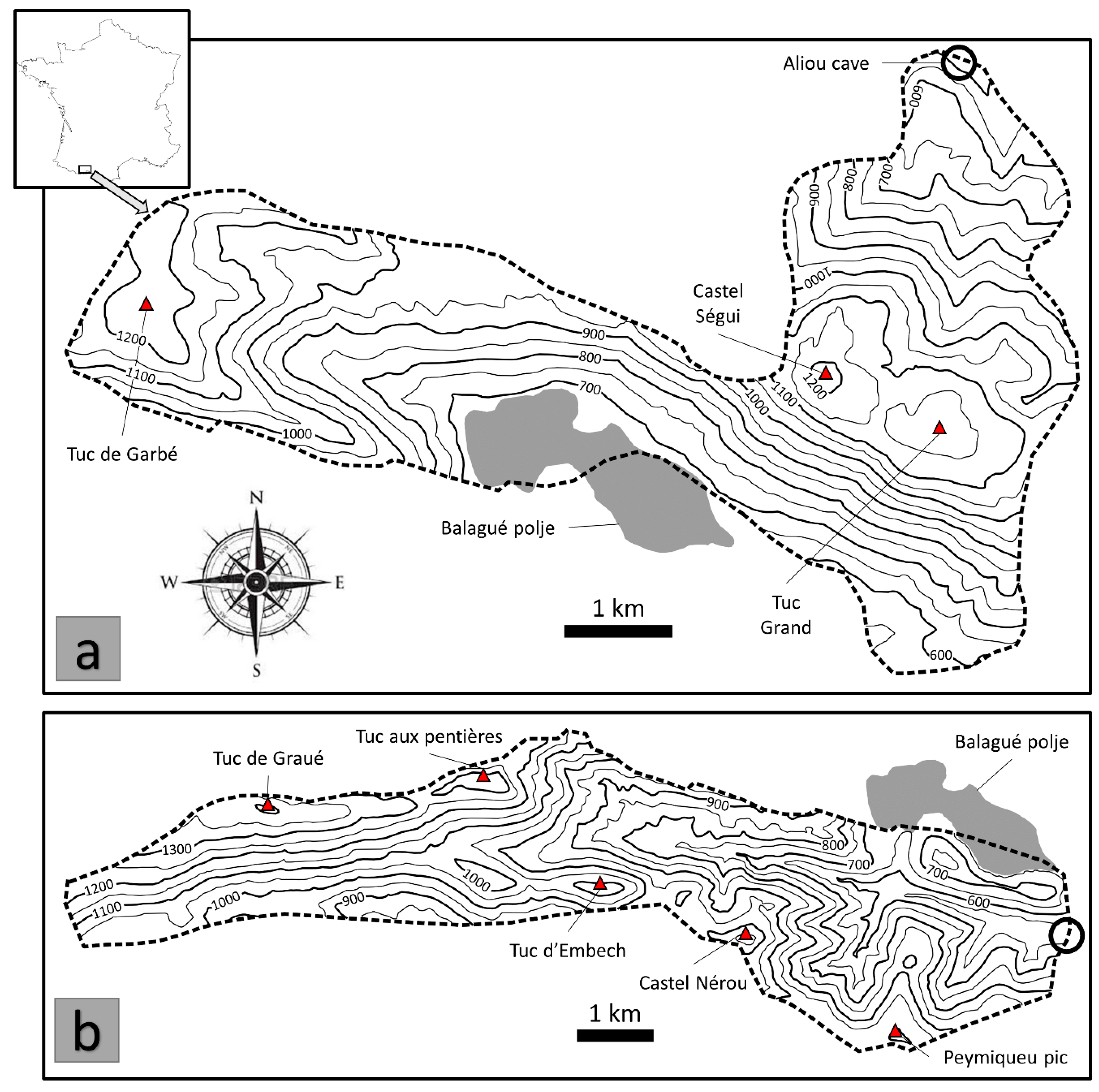
We studied field data from two karstic springs of the French Pyrenees Mountains (Ariège): the Aliou and the Baget watersheds (Figure 1). These two watersheds share a common median altitude of 1000 m and the recharge area are respectively estimated at about 11.9 km2 and 13.2 km2 [4]. They belong to the carbonated belt bordering the north of the French Pyrenees. The two systems share a common boundary oriented west-east. South of this boundary, the Baget area is affected by the Alas fault: Jurassic to Cretaceous metamorphic limestone dips 45° to 75° under slaty flysch on the southern border. The valley follows the contact between karstified calcareous formations and impervious flysch oriented in a west-east direction. Jurassic and Palaeozoic metamorphic dolomite and flysch constitute the northern border of the watershed. This corresponds to the Sainte-Suzanne marls, playing the role of a tight barrier. North of this barrier, the Aliou watershed is composed of Aptian limestone. The drainage is done in a north-south direction until the outlet located in the Aliou cave.
The meteorological data are measured by Météo-France in the station of Antichan (Pyrenees) on both a daily and hourly sampling rate. Considering the respective geographical locations and the available meteorological data, we decided to consider the same rainfall time series for both watersheds. Both watersheds have never been instrumented in order to get local value of the evapotranspiration on this mountainous area. Without this kind of measurement, estimation of a real evapotranspiration constitutes a complex task, giving more uncertainty in the modeling especially when moving from a daily time step to an hourly time step. Then we choose to neglect the evapotranspiration as it is not possible to consider it in proper way.
Aliou and Baget karstic systems are monitored since the late 1970s [31] with daily measurement of the outlet discharge and hourly measurements since the early 1990s [14]. The hourly time series presents some gaps [30]. Here, we focus on common periods in order to properly compare flow dynamics in the two studied watersheds. Both Aliou and Baget are responsive hydro-systems. Based on hourly discharge time series, the memory effects [31] have been estimated to be 70 h and 110 h respectively. Also, the cross-correlation function between hourly rainfalls and spring discharge time series show a peak value on 7 h for Aliou and 14 h for Baget. Both watersheds are subject to quick infiltration and a rapid transit time between infiltration points and the outlet. Preliminary statistics highlights the interest in working with sub-daily time series. Moreover, these systems are classified as well karstified watersheds with highly developed speleological networks [4].
2.2. Modeling Approach
2.2.1. Conceptual Reservoir Modeling
The KarstMod modeling platform [27,28] is a conceptual reservoir model dedicated to karstic groundwater flow simulation. This model is developed by the French institution INSU-CNRS SNO KARST [32]. It consists of a modular “bucket-style” conceptual model that enables us to build a structured assembly of interconnected reservoirs and to quantify water fluxes between reservoirs in several time steps. In its most complex form, the platform offers 4 compartments organized as a two-level structure: (1) compartment E (higher level) and (2) compartments L, M and C (lower level). A priori, the higher-level stands for the infiltration zone, and the lower level stand for the saturated zone where compartment L, M, and C stand for the different sub-systems of the saturated zone. The rainfall, noted as P, and the evapotranspiration, noted as ET, only impact the reservoir E. Then the water flows towards the deep reservoirs C, M, and L or is lost to the system. The KarstMod model has been successfully applied to the Norville chalk aquifer [33], Dardenne’s spring [34] and Fontaine de Vaucluse [28]. Also, it constitutes a valuable tool for hydrodynamic analysis in a context of intrinsic vulnerability and pollution risk mapping [35] or even for the assessment of the vadose zone contribution in the groundwater recharge [36]. Furthermore, the KarstMod platform (http://www.sokarst.org/) allows high flexibility in karstic groundwater flow modeling with the possibility to include, where appropriate, pumping discharge and loss.
The KarstMod model is based on the mass-balance equations given by Mazzilli et al. [28]:
where:
where P and ET are respectively rainfall and evapotranspiration (L), E(t), M(t) and C(t) are the water levels in the reservoirs E (epikarst), M (matrix) and C (conduit), kAB is the recession coefficient associated with the flow from reservoir A (either E, M, or C) to reservoir B (either M, C, or L) or to the outlet S and QAB (L/T) is the discharge from A to B. Discharge in (L3/T) is computed by the product of QAB with the total surface of the recharge area (RA).
Here, the L reservoir is not used as both Aliou and Baget are very responsive watersheds. To reproduce the different flow behavior between epikarst (E) and the deeper reservoirs conduit (C) and matrix (M), emptying exponents are fixed as aEM = aMC = 1, aEC = 2 and aCS = 4. Then we assume turbulent flow with non-linear law in conduit and capillary flow with linear law in the matrix. Both Aliou and Baget karstic watersheds are well karstified and conduit dominated with a short memory effect [31]. The emptying exponent between reservoir M and C is chosen to be equal to the emptying coefficient for E to M as the exchange between the conduit and the surrounding matrix is mainly determined by the hydraulic conductivity of the fissured system [37]. To give better physical realism to the model, it has been chosen to set all output discharge rate through reservoir C (Figure 2) Also, previous studies have shown that the rainfall-runoff relationship for both Aliou and Baget watersheds may be correctly described by making ET equal to zero [14,38,39].
2.2.2. Model Calibration
The rainfall-discharge model is calibrated using a quasi-Monte-Carlo procedure with a Sobol sequence sampling of the parameter space [28]. The best parameters set for the model are chosen as the ones that maximize the performance criteria. Here, it corresponds to a weighted sum of a classical Nash-Sutcliff efficiency NSE [40] and a modified balance error BE [41].
where qsim is the discretized time series simulated by the model, and qobs is the discretized experimental time series measured in the field. The NSE criterion is fluently used to judge the quality of a rainfall-runoff model [28,34,42,43]. Nonetheless, this criterion tends to favor the conformity of the model for the strong discharge values to the detriment of the weakest ones. Introducing a balance error estimation allows us to better describe the quality of the model in the case where overestimation of discharge during low water could introduce important mass errors between observed and simulated data. Also, the effects of bias introduced by some conditions such as large events can be reduced by data transformation [44] or by including the bias as an explicit component, as for the Kling-Gupta efficiency KGE [45]. Here the optimization function Wobj is defined such as:
The KarstMod model is warmed, calibrated and validated considering periods shown in Table 1. As such, the model is warmed over 2 years, calibrated over 10 years and validated over 36 years for the daily time series (corresponding to 17,898 successive data). In the same way, the model for hourly time series is warmed over 1 year, calibrated over 2 years and validated over 5 years (corresponding to 67,200 successive data). So, the warm-up period is long enough to ensure the calibration independence from initial conditions. Also, this allows a good balance between the number of calibration and validation data with a validation period at least two times longer than the calibration period [26,34].
2.2.3. Scale Effects
The temporal resolution of hydrological models has been widely discussed during the past decades [46,47,48], in the context of scaling of regional flood frequency [49,50]. The transformation of rainfall into streamflow includes several processes with characteristic time covering several orders of magnitude [46]. Then, the sampling rate must be suitable in the range of time and space scale if the physical phenomenon was to take place. For example, at small catchment scales, within-storm patterns of rainfall variability are important, while at large catchment scales, longer timescales such as seasonality are dominant [49]. According to Ficchi et al., [47] the proper description and simulation of these processes requires a short time step for at least three reasons: (1) the short duration of runoff events (e.g., flash floods); (2) the considerable intra-storm variability that control some runoff processes and (3) the integration of differential equations in the model structure (numerical reason). A low sampling frequency may numerically increase the catchment response time and leads to a bad description of time dependence between rainfall and spring discharge. This gives rise to a phenomenon which can be described as representing a space to time connection—a spatial scaling behavior which is generated by the interactions in the time domain between rainfall and runoff processes. So, considering rainfall-runoff relationships at the catchment scale in a karstic system with a small recharge area needs high-resolution monitoring. Previous studies have already shown interest in a high-resolution monitoring of the Aliou and Baget watersheds [12,14,30].
3. Results and Discussion
The KarstMod model has been calibrated and validated on both Aliou and Baget karstic watersheds. As these two systems show strong similarities in terms of size, morphology, and lithology, the same model structure has been chosen (Figure 2). All information about model parameters, and about performance criterion has been respectively reported in Table 2 and Table 3. The model is calibrated on both hourly and daily time series, allowing us to study the internal flow over different observations scale: (1) the hourly monitored time series allow a better description of the physical processes at the flood event scale and (2) the daily monitored time series measured over 50 years allow us to identify long-term trends in the internal fluxes and in the reservoirs water level.
3.1. Short-term Varibility of Internal Fluxes
Several studies have shown interest in assessing the flow dynamics between the main drainage structure and the surrounding matrix at a flood event scale [51]. This is a key point when dealing with short-term solute transport and testing source pollution scenarios. Indeed, considering the internal flow dynamics allows us to better quantify the potential consequences of pollutions. In case of the existence of a hydraulic gradient between the conduit and the surrounding matrix part of the contaminant may be temporally stored in so-called “dead space” [52]. This has been investigated at a laboratory scale [53,54] but remains badly constrained in real karst systems. Then, a well-constrained flow partition between different flow compartments can be useful for solute transport modeling. This point may help to improve the application of an Advection-Dispersion Equation (ADE) approach where the discharge is often considered to be the spring discharge [55]. Recent studies have shown interest in discretizing transport along the flow path [51,56]. Also, solute transport modeling can be improved with a well-constrained balance of exchange between the main drainage structures and the surrounding matrix [57].
The KarstMod modeling platform was used to model Aliou and Baget karstic systems on hourly time-steps to assess the ability of the model to give physically significant internal flow dynamics. As the dynamics in karst aquifers may vary on several orders of magnitude, one needs monitoring with a sufficiently high frequency to correctly characterize the variability of the flow dynamics over a flood event. For instance, flood event in karst aquifers such as Fontaine de Vaucluse [25] can be correctly characterized based on daily time series. But assessing flow dynamics on a highly karstified watershed, with the short-term response, needs monitoring at a higher frequency, as it is the case for Aliou and Baget watersheds [30].
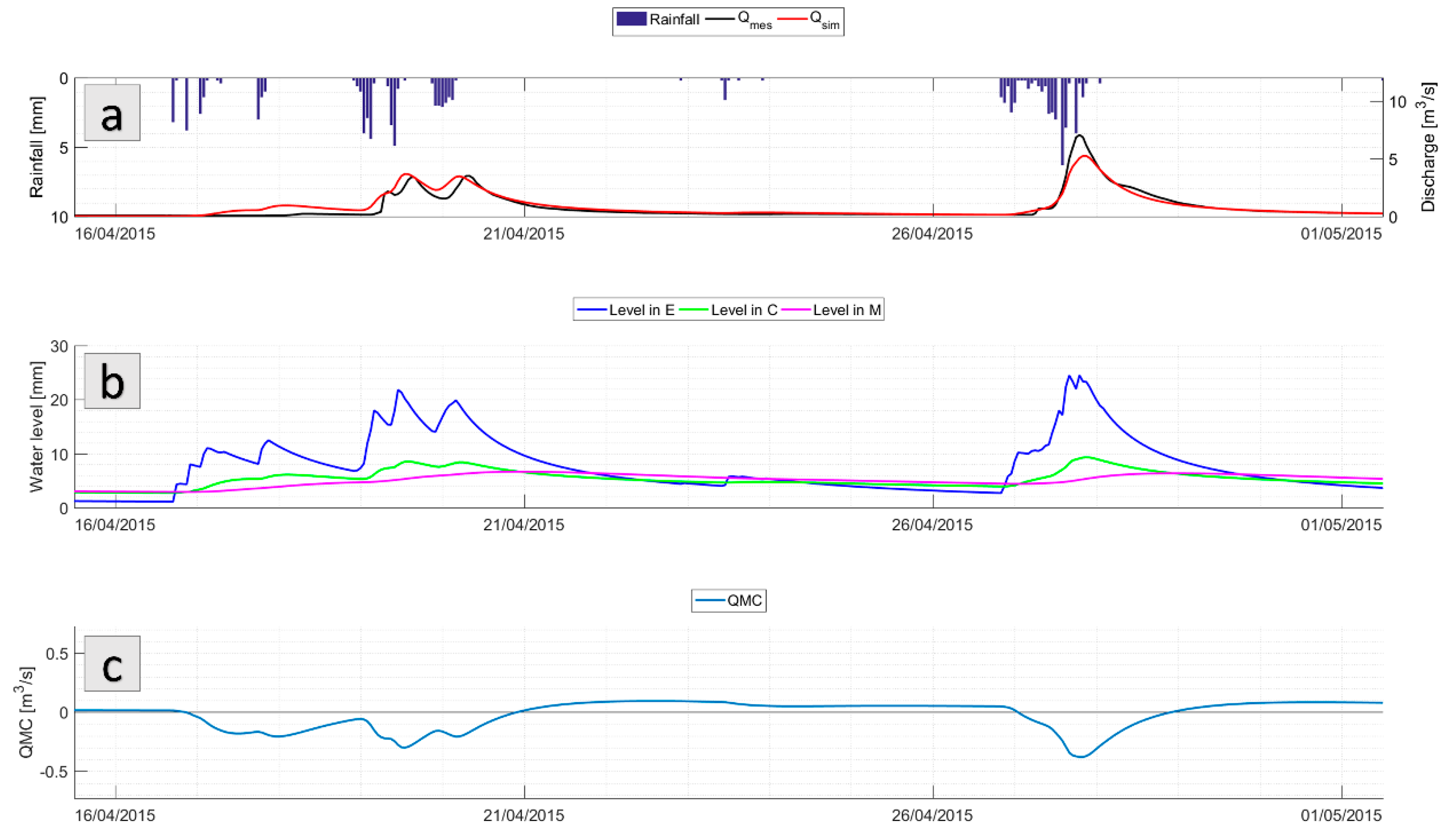
Figure 3 shows part of the KarstMod model time series for Aliou watershed from 16 April 2015 to 2 May 2015. The rainfall time series is mainly composed of two rainfall events separated by six days. During the first rainfall event (19 and 20 April 2015), the water level in reservoir E (epikarst) rises quickly and most of the water goes to the reservoir C. On the same time interval, QMC shows negative values, which means that the reservoir C feeds the reservoir M. Then, at the end of the rainfall event, the water level in all reservoir drops with different dynamics and after about two days without rainfall, the fluxes between reservoir M and C change direction. Then, the reservoir M feeds the reservoir C during recessional, until the next rainfall event (i.e., new water input in the system). These event scale dynamics are consistent with results obtained with a physically-based approach [58,59]. Nonetheless, these approaches need a correct knowledge of flow geometry to give a reliable discretization of the flow path in so-called “reach” were flow and transport parameters may be considered as homogeneous. The matrix-conduit dynamic had also been highlighted using conceptual modeling [60]. Duran [33] highlighted the dynamic fluxes between the conduit and a surrounding matrix over the Norville chalk aquifer using a KarstMod model coupled with turbidity and electrical conductivity analysis. In the study by Duran [33], the fluxes QMC represent about 10% of the spring discharge. Over the Baget and Aliou watersheds, the contribution of the fluxes QMC in the spring discharge is in the same order of magnitude. Zhang et al., [61] proposed a conceptual model coupled with dissolution rates estimations in “slow flow” and “fast flow” systems. They estimated the contribution of exchange from “slow flow” to “fast flow” systems in three catchments to vary between 64.1% and 87.5%.
3.2. Long-Term Variability of Internal Dynamics
The next step consists of assessing the effect of inter-annual variability of rainfall on both internal fluxes and water levels in the considered reservoirs (E, M, and C) of the KarstMod model. Here, we focus more especially on how the internal drainage system interacts with the surrounding long-term storing aquifer. To do so, the analysis focuses on the matrix-conduit exchanges and on the reservoir M storage capacity. Then, analyzing the evolution of water level over 5 decades, coupled with rainfall analysis, allow us to assess the effects of long-term trends on water supply.
To study seasonal patterns and inter-annual variability, Anghileri et al. [62] introduced the MASH method (Moving Average over Shifting Horizon) involving mobile averaging across both the day of the year and year of the time series to allow trend detection. So, the MASH method needs to define only two parameters (i.e., number of days for seasonal pattern detection and number of years for inter-annual pattern). As the MASH methods do not provide specific recommendations about its two parameter values, several options have been tested and the best solution is presented here: the method was applied in such a way that seasonal pattern is evidenced by a 2-month centred moving average of the times series whereas inter-annual pattern is evidenced by a 15-year shifting horizon. This configuration gives a satisfactory balance between detection of seasonal patterns and inter-annual patterns for each of the variable of interest in this study: rainfall, spring discharge and the water level in reservoir M.
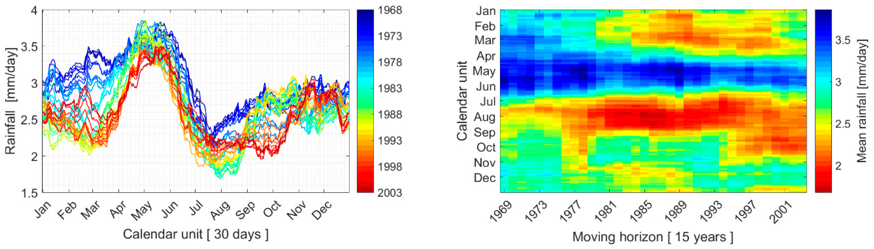
The MASH method is first applied to the daily rainfall time’s series, which ranges from 1 January 1969 to 31 December 2016. As a reminder, both Aliou and Baget models are fed by the same rainfall time series. The moving average along the day of the year is shown for the years 1968 to 2016 (Figure 4—left). The corresponding curves are coloured from blue for the oldest to red for the more recent periods. Considering the daily rainfall time series, the MASH analysis shows that the mean rainfall decreased during the past decades. This decrease appears to be more important during the early spring season, with a mean rainfall rate decreasing from 3.5 mm/day to 2.1 mm/day and during summer, with a mean rainfall rate decreasing from 2.5 mm/day to 1.7 mm/day. Also, rainfalls seem to be smoothed during late summer and early autumn periods, with a mean rainfall rate about 2 mm/day whereas oldest decades show a certain variability from about 1.8 mm/day in August to 2.6 mm/day in October. Then, winter appeared to be drier from the 1980s onwards and the rain deficit during summer has appeared to last longer since the 1990s (Figure 4—right). Nonetheless, one should keep in mind the strong smoothing effect of the MASH method: it gives only global trend effects and does not provide information about the rainfall event intensity and their temporal repartition.
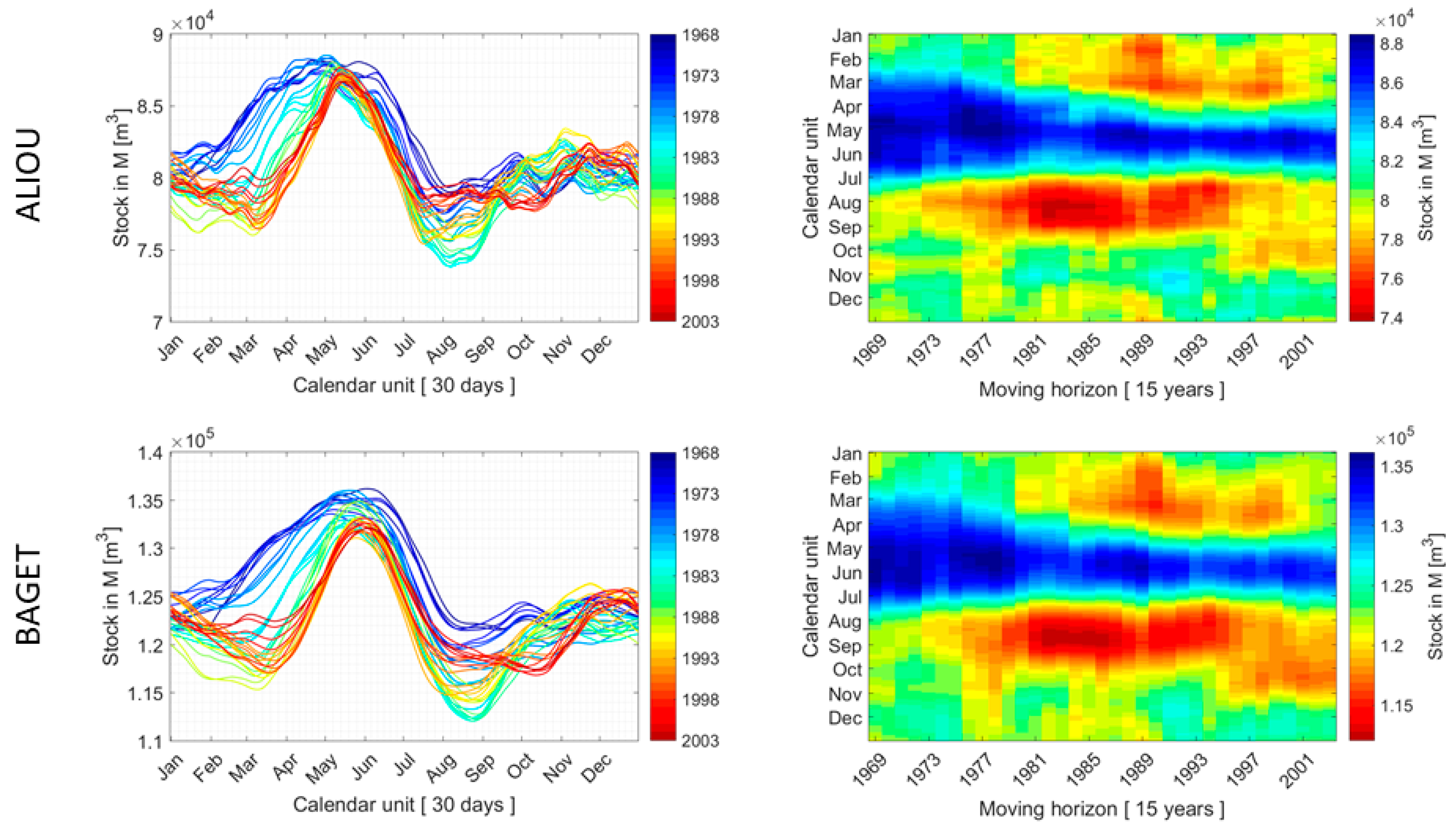
Then, the MASH method is applied to the reservoir M water level time series, inferred from the KarstMod model, on Aliou and Baget (Figure 5). The MASH method highlighted an important decrease in the water level during spring periods since the 1960s (Figure 5—left). It represents about −13.1 % for Aliou and −11.3% for Baget. The annual recharge seemed to occur later during the hydrological cycle: recharge now seemed to start in April since the early 1990s, whereas it apparently used to begin in February from 1968 up to the early 1990s (Figure 5—left). The total water volume calculated in the M reservoir is in the same order of magnitude as the dynamic volume calculated based on the analyses of the recessional curve [4].
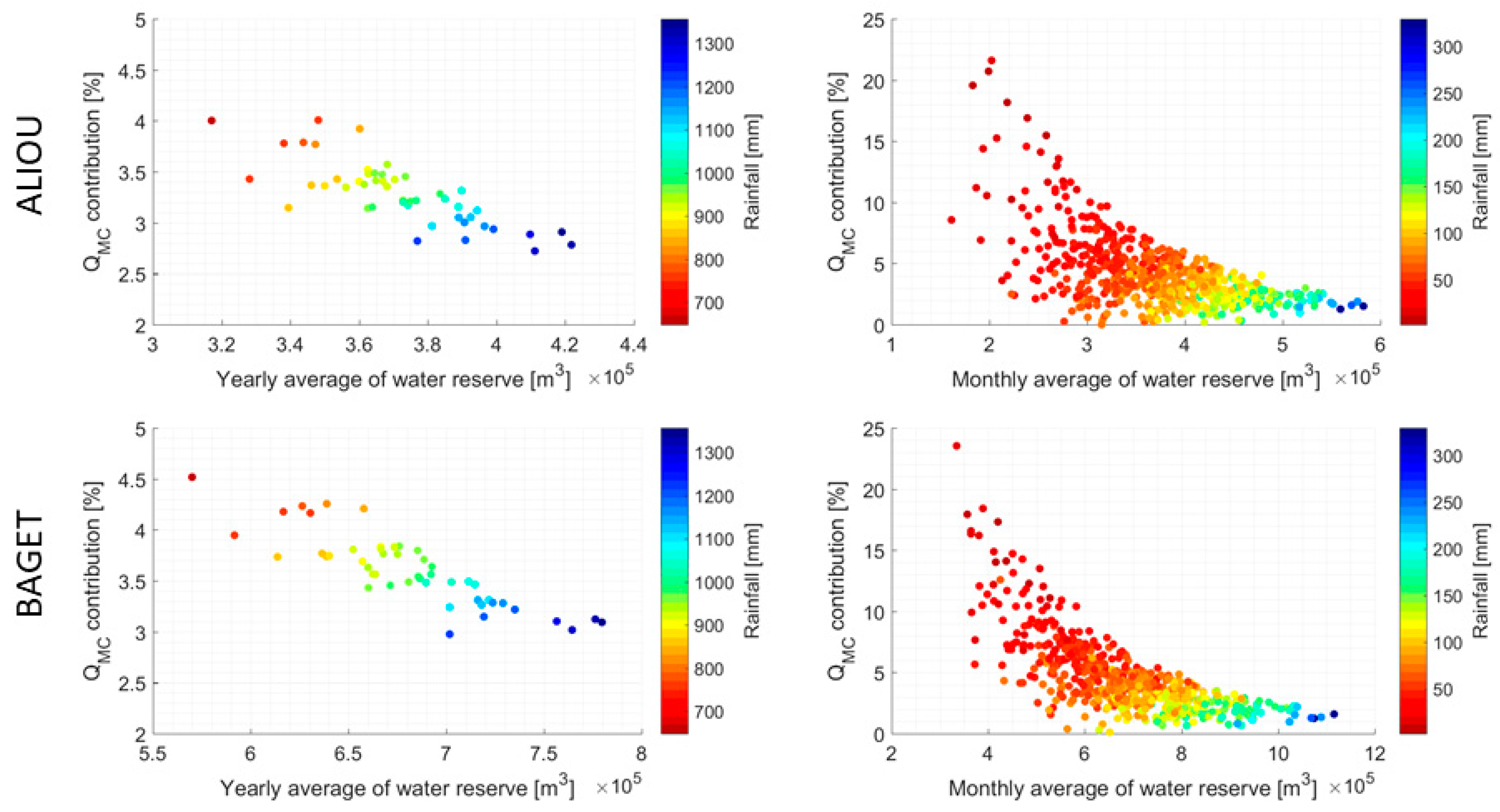
Finally, the contribution of the flow from the matrix to the conduit was assessed by computing a water balance defined as the ratio of the volume of exchange between reservoir M and C to the total volume flowing out of the system. It was then possible to determine the proportion of the water volume flowing through the matrix before coming out of the system (Figure 6). The results showed that the contribution of water coming from the matrix to the conduit to total spring discharge. This contribution varied from about 2% to 5% over a complete year, can increase up to 25% over a month, and seemed to be well constrained with the water level in M reservoir and the total inflow (cumulative rainfall). Also, the more important the contribution of M reservoir to total spring outflow, the lower the water level in reservoir M and the lower the inflows (cumulative rainfalls). This means that the system tends to drain rainfall inflows directly through reservoir C to the outlet when the reservoir M is already filled. In contrast, during dry periods the contribution of the matrix increases and entirely accounts for spring base-flow.
Calibration of the KarstMod model over long periods (i.e., several years) may provide robust long-term flow behavior modeling (i.e., validation over several decades). The model proposed here has been calibrated over one decade and validated over four decades. This allowed a long-term description of internal flow dynamics and may provide a valuable source of information to assess the effect of climate variability and changes on karst system water supply. This is a major issue for water management and water security for the future. It is estimated that one-quarter of the world’s population depends on freshwater from karst aquifers [2]. Also, the environment is subject to natural and anthropogenic changes leading to an increase of imbalance between freshwater supply and needs for a growing population [63]. So, providing efficient models to predict evolutions of water resources constitutes a major challenge for hydrological sciences [18,64]. Otherwise, those models may include, where appropriate, special features about the impacts of change in land use [29,65].
4. Conclusions
A reservoir model based on KarstMod modeling platform has been applied on two highly karstified watersheds with small recharge area (~10 km2) in order to assess the dynamics of internal flow and water levels in the different compartments of the watershed (i.e., Epikarst, Matrix, and Conduit). The modeling has been conducted for two different time steps. Based on this modeling approach, hydrodynamics relationships between reservoirs M and C (representative of the matrix with slow flow and the conduit with fast flow and non-linear behavior, respectively) have been more preferentially explored on the short-term scale (i.e., a rainfall event) and on the long-term scale (i.e., inter-annual scale).
The KarstMod model appeared to be an efficient way to model the internal flow dynamics in highly karstified watersheds and allowed characterizing flux inversions between conduit and matrix over successive rainfall events. The internal flow dynamics highlighted here with a conceptual model appeared to be consistent with results obtained from physically-based approaches and hydrochemical studies [58,61]. Moreover, the estimated volume of water available in the matrix compartment was of the same order of magnitude as the dynamic volume estimated through recession curve analysis [4]. It is estimated that the matrix would contribute up to 25% of the total monthly spring discharge during periods with low rainfall. This contribution would decrease to about 3% when there are important rainfalls. Therefore, the main part of the watershed drainage is operated by reservoir C (i.e., fast flow and nonlinear behavior).
Moreover, long-term trends in water levels have been assessed using the moving average over the shifting horizon method [62]. It is estimated that the mean water level during spring periods decreased by 13.1% for Aliou and 11.3% for Baget. Also, the recharge of the aquifers appears to occur later during the hydrological cycle: recharge has appeared to start in April since the early 1990s, whereas it apparently used to begin in February between 1968 up to the early 1990s. This kind of information can be of major interest for water management and water security, as it gives an overview of recharge processes and gives an estimation of the water volume stored in the aquifer. Also, the KarstMod modeling approach coupled with the MASH analysis can be extended to assess the effects of the climate changes.
Author Contributions
Conceptualization, V.S.; Methodology, V.S. and D.L.; Software, N.M. (Naomi Mazzilli); Validation, N.M. (Nicolas Massei), N.M. (Naomi Mazzilli) and H.J.; Formal Analysis, V.S.; Investigations, V.S. and D.L.; Resources, V.S. and D.L.; Data Curation, D.L.; Writing-Original Draft, V.S.; Writing-Review & Editing, D.L., N.M. (Nicolas Massei), N.M. (Naomi Mazzilli) and H.J.; Supervision, D.L.
Funding
This research received no external funding.
Acknowledgments
The authors would like to thank the KARST observatory network (SNO KARST) initiative at the INSU/CNRS, which aims to strengthen knowledge sharing and promote cross-disciplinary research on karst systems at the national scale. We also thank Météo-France for providing rainfall data and BRGM (French geological survey) for providing recent discharge data. We also would like to dedicate this contribution to the memory of Alain Mangin and to his long-term invaluable care of collecting data on these two Pyreneans watersheds.
Conflicts of Interest
The authors declare no conflict of interest.
References
- Quinif, Y. Karst et évolution des rivières: Le cas de l’Ardenne. Geodin. Acta 1999, 12, 267–277. [Google Scholar] [CrossRef]
- Ford, D.; Williams, P.D. Karst Hydrogeology and Geomorphology; John Wiley & Sons, Inc.: Hoboken, NJ, USA, 2007; ISBN 978-0-470-84996-5. [Google Scholar]
- Kiraly, L. Karstification and groundwater flow. Speleogenesis Evol. Karst Aquifers 2003, 1, 26. [Google Scholar]
- Mangin, A. Contribution à l’étude Hydrodynamique des Aquifères Karstiques. Ph.D. Thesis, Université de Bourgogne, Dijon, France, 1975. [Google Scholar]
- Marsaud, B. Structure et Fonctionnement de la Zone Noyée des Karsts à Partir des Résultats Expérimentaux. Ph.D. Thesis, Université de Paris XI Orsay, Paris, France, 1997. [Google Scholar]
- Klimchouk, A. Karst morphogenesis in the epikarstic zone. Cave Karst Sci. 1995, 21, 45–50. [Google Scholar]
- Batiot, C.; Emblanch, C.; Blavoux, B. Total Organic Carbon (TOC) and magnesium (Mg2+): Two complementary tracers of residence time in karstic systems. Comptes Rendus Geosci. 2003, 335, 205–214. [Google Scholar] [CrossRef]
- Emblanch, C.; Zuppi, G.; Mudry, J.; Blavoux, B.; Batiot, C. Carbon 13 of TDIC to quantify the role of the unsaturated zone: The example of the Vaucluse karst systems (Southeastern France). J. Hydrol. 2003, 279, 262–274. [Google Scholar] [CrossRef]
- Garry, B. Etude des Processus d’écoulements de la Zone non Saturée Pour la Modélisation des Aquifères Karstiques: Expérimentation Hydrodynamique et Hydrochimique sur les Sites du Laboratoire Souterrain à Bas Bruit (LSBB) de Rustrel et de Fontaine de Vauclusee. Ph.D. Thesis, Université d’Avignon et des pays de Vaucluse, Avignon, France, 2007. [Google Scholar]
- Lastennet, R. Rôle de la Zone non Saturée Dans le Fonctionnement des Aquifères Karstiques. Approche par l’étude Physico-Chimique et Isotopique du Signal D’entrée et des Exutoires du Massif du Ventoux (Vaucluse). Ph.D. Thesis, Université d’Avignon et des pays de Vaucluse, Avignon, France, 1994. [Google Scholar]
- Puig, J.-M. Le système Karstique de la Fontaine de Vaucluse. Ph.D. Thesis, Université d’Avignon et des pays de Vaucluse, Avignon, France, 1987. [Google Scholar]
- Labat, D.; Hoang, C.T.; Masbou, J.; Mangin, A.; Tchiguirinskaia, I.; Lovejoy, S.; Schertzer, D. Multifractal behavior of long-term karstic discharge fluctuations. Hydrol. Process. 2013, 27, 3708–3717. [Google Scholar] [CrossRef]
- Labat, D.; Ababou, R.; Mangin, A. Analyse multirésolution croisée de pluies et débits de sources karstiques. Comptes Rendus Géosc. 2002, 334, 551–556. [Google Scholar] [CrossRef]
- Labat, D.; Mangin, A.; Ababou, R. Rainfall–runoff relations for karstic springs: Multifractal analyses. J. Hydrol. 2002, 256, 176–195. [Google Scholar] [CrossRef]
- Labat, D.; Ababou, R.; Mangin, A. Introduction of wavelet analyses to rainfall/runoffs relationship for karstic basin: The case of Licq-Atherey karstic system (France). Ground Water 2001, 39, 605–615. [Google Scholar] [CrossRef]
- Ficchi, A. An adaptative Hydrological Model for Multiple Time-Steps: Diagnostics and Improvements Based on Fluxes Consistency. Ph.D. Thesis, Université Pierre et Marie Curie, Paris, France, 2017. [Google Scholar]
- Harbaugh, A.W. MODFLOW-2005, the U.S. Geological Survay Modular Ground-Water Model-the Ground-Water Flow Process; U.S. Geological Survey Techniques and Methods 6-A16; U.S. Geological Survey: Reston, VA, USA, 2005.
- Hartmann, A.; Goldscheider, N.; Wagener, T.; Lange, J.; Weiler, M. Karst water resources in a changing world: Review of hydrological modeling approaches. Rev. Geophys. 2014, 52, 218–242. [Google Scholar] [CrossRef]
- Chen, Z.; Goldscheider, N. Modeling spatially and temporally varied hydraulic behavior of a folded karst system with dominant conduit drainage at catchment scale, Hochifen–Gottesacker, Alps. J. Hydrol. 2014, 514, 41–52. [Google Scholar] [CrossRef]
- Denić-Jukić, V.; Jukić, D. Composite transfer functions for karst aquifers. J. Hydrol. 2003, 274, 80–94. [Google Scholar] [CrossRef]
- Weiler, M.; McGlynn, B.L.; McGuire, K.J.; McDonnell, J.J. How does rainfall become runoff? A combined tracer and runoff transfer function approach. Water Resour. Res. 2003, 39, 1315. [Google Scholar] [CrossRef]
- Cormary, Y.; Guilbot, A. Ajustement et réglage des modèles déterministes méthode de calage des paramètres. La Houille Blanche 1971, 2, 131–140. [Google Scholar] [CrossRef]
- Bezes, C. Contribution à la Modélisation des Systèmes Aquifères Karstiques: Établissement du Modèle Bemer, Son Application à Quatre Systèmes Karstiques du Midi de la France; CERGA: Montpellier, France, 1976. [Google Scholar]
- Thiéry, D. Logiciel GARDIENA Version 8.2: Guide d’utilisation; BRGM: Orléans, France, 2016; p. 126, 65 fig., 2ann; Available online: https://www.brgm.fr/sites/default/brgm/logiciels/gardenia/GARDENIA_v8_2_RP-62797-FR_Notice.pdf (accessed on 18 March 2019).
- Fleury, P.; Plagnes, V.; Bakalowicz, M. Modelling of the functioning of karst aquifers with a reservoir model: Application to Fontaine de Vaucluse (South of France). J. Hydrol. 2007, 345, 38–49. [Google Scholar] [CrossRef]
- Tritz, S.; Guinot, V.; Jourde, H. Modelling the behavior of a karst system catchment using non-linear hysteretic conceptual model. J. Hydrol. 2011, 397, 250–262. [Google Scholar] [CrossRef]
- Jourde, H.; Mazzilli, N.; Lecoq, N.; Arfib, B.; Bertin, D. KarstMod: A Generic Modular Reservoir Model Dedicated to Spring Discharge Modeling and Hydrodynamic Analysis in Karst. In Hydrogeological and Environmental Investigations in Karst Systems; Environmental Earth Sciences; Springer: Berlin/Heidelberg, Germany, 2015; pp. 339–344. ISBN 978-3-642-17434-6. [Google Scholar]
- Mazzilli, N.; Guinot, V.; Jourde, H.; Lecoq, N.; Labat, D.; Arfib, B.; Baudement, C.; Danquigny, C.; Dal Soglio, L.; Bertin, D. KarstMod: A modelling platform for rainfall—Discharge analysis and modelling dedicated to karst systems. Environ. Model. Softw. 2017. [Google Scholar] [CrossRef]
- Bittner, D.; Narany, T.S.; Kohl, B.; Disse, M.; Chiogna, G. Modeling the hydrological impact of land use change in a dolomite-dominated karst system. J. Hydrol. 2018, 567, 267–279. [Google Scholar] [CrossRef]
- Labat, D.; Masbou, J.; Beaulieu, E.; Mangin, A. Scaling behavior of the fluctuations in stream flow at the outlet of karstic watersheds, France. J. Hydrol. 2011, 410, 162–168. [Google Scholar] [CrossRef]
- Mangin, A. Pour une meilleure connaissance des systèmes hydrologiques à partir des analyses corrélatoire et spectrale. J. Hydrol. 1984, 67, 25–43. [Google Scholar] [CrossRef]
- Jourde, H.; Massei, N.; Mazzilli, N.; Binet, S.; Batiot-Guilhe, C.; Labat, D.; Steinmann, M.; Bailly-Comte, V.; Seidel, J.L.; Arfib, B.; et al. SNO KARST: A French Network of Observatories for the Multidisciplinary Study of Critical Zone Processes in Karst Watersheds and Aquifers. Vadose Zone J. 2018, 17. [Google Scholar] [CrossRef]
- Duran, L. Approche Physique, Conceptuelle et Statistique du Fonctionnement Hydrologique d’un Karst sous Couverture. Ph.D. Thesis, Université de Rouen, Rouen, France, 2015. [Google Scholar]
- Baudement, C.; Mazzilli, N.; Jouves, J.; Guglielmi, Y. Groundwater Management of a Highly Dynamic Karst by Assessing Baseflow and Quickflow with a Rainfall-Discharge Model (Dardennes Springs, SE France). Bull. Soc. Géol. Fr. 2017, 188, 40. [Google Scholar] [CrossRef]
- Kazakis, N.; Chalikakis, K.; Mazzilli, N.; Ollivier, C.; Manakos, A.; Voudouris, K. Management and research strategies of karst aquifers in Greece: Literature overview and exemplification based on hydrodynamic modelling and vulnerability assessment of a strategic karst aquifer. Sci. Total Environ. 2018, 643, 592–609. [Google Scholar] [CrossRef] [PubMed]
- Poulain, A.; Watlet, A.; Kaufmann, O.; Camp, M.V.; Jourde, H.; Mazzilli, N.; Rochez, G.; Deleu, R.; Quinif, Y.; Hallet, V. Assessment of groundwater recharge processes through karst vadose zone by cave percolation monitoring. Hydrol. Process. 2018, 32, 2069–2083. [Google Scholar] [CrossRef]
- Bauer, S.; Liedl, R.; Sauter, M. Modeling of karst aquifer genesis: Influence of exchange flow. Water Resour. Res. 2003, 39. [Google Scholar] [CrossRef] [Green Version]
- Labat, D.; Ababou, R.; Mangin, A. Rainfall–runoff relations for karstic springs. Part I: Convolution and spectral analyses. J. Hydrol. 2000, 238, 123–148. [Google Scholar] [CrossRef]
- Labat, D.; Ababou, R.; Mangin, A. Rainfall–runoff relations for karstic springs. Part II: Continuous wavelet and discrete orthogonal multiresolution analyses. J. Hydrol. 2000, 238, 149–178. [Google Scholar] [CrossRef]
- Nash, J.E.; Sutcliffe, J.V. River flow forecasting through conceptual models part I—A discussion of principles. J. Hydrol. 1970, 10, 282–290. [Google Scholar] [CrossRef]
- Perrin, C.; Michel, C.; Andréassian, V. Does a large number of parameters enhance model performance? Comparative assessment of common catchment model structures on 429 catchments. J. Hydrol. 2001, 242, 275–301. [Google Scholar] [CrossRef]
- Charlier, J.-B.; Bertrand, C.; Mudry, J. Conceptual hydrogeological model of flow and transport of dissolved organic carbon in a small Jura karst system. J. Hydrol. 2012, 460–461, 52–64. [Google Scholar] [CrossRef]
- Hartmann, A.; Barberá, J.A.; Lange, J.; Andreo, B.; Weiler, M. Progress in the hydrologic simulation of time variant recharge areas of karst systems—Exemplified at a karst spring in Southern Spain. Adv. Water Resour. 2013, 54, 149–160. [Google Scholar] [CrossRef]
- Bennett, N.D.; Croke, B.F.W.; Guariso, G.; Guillaume, J.H.A.; Hamilton, S.H.; Jakeman, A.J.; Marsili-Libelli, S.; Newham, L.T.H.; Norton, J.P.; Perrin, C.; et al. Characterising performance of environmental models. Environ. Model. Softw. 2013, 40, 1–20. [Google Scholar] [CrossRef]
- Gupta, H.V.; Kling, H.; Yilmaz, K.K.; Martinez, G.F. Decomposition of the mean squared error and NSE performance criteria: Implications for improving hydrological modelling. J. Hydrol. 2009, 377, 80–91. [Google Scholar] [CrossRef] [Green Version]
- Blöschl, G.; Sivapalan, M. Scale issues in hydrological modelling: A review. Hydrol. Process. 1995, 9, 251–290. [Google Scholar] [CrossRef]
- Ficchì, A.; Perrin, C.; Andréassian, V. Impact of temporal resolution of inputs on hydrological model performance: An analysis based on 2400 flood events. J. Hydrol. 2016, 538, 454–470. [Google Scholar] [CrossRef]
- Wang, Y.; He, B.; Takase, K. Effects of temporal resolution on hydrological model parameters and its impact on prediction of river discharge/Effets de la résolution temporelle sur les paramètres d’un modèle hydrologique et impact sur la prévision de l’écoulement en rivière. Hydrol. Sci. J. 2009, 54, 886–898. [Google Scholar] [CrossRef]
- Jothityangkoon, C.; Sivapalan, M. Temporal scales of rainfall-runoff processes and spatial scaling of flood peaks: Space-time connection through catchment water balance. Adv. Water Resour. 2001, 24, 1015–1036. [Google Scholar] [CrossRef]
- Robinson, J.S.; Sivapalan, M. An investigation into the physical causes of scaling and heterogeneity of regional flood frequency. Water Resour. Res. 1997, 33, 1045–1059. [Google Scholar] [CrossRef] [Green Version]
- Cholet, C. Fonctionnement Hydrogéologique et Processus de Transport dans les Aquifères Karstiques du Massif du Jura. Ph.D. Thesis, Université de Bourgogne Franche-Comté, Besançon, France, 2017. [Google Scholar]
- Goldscheider, N. A new quantitative interpretation of the long-tail and plateau-like breakthrough curves from tracer tests in the artesian karst aquifer of Stuttgart, Germany. Hydrogeol. J. 2008, 16, 1311–1317. [Google Scholar] [CrossRef] [Green Version]
- Li, G.; Loper, D.E.; Kung, R. Contaminant sequestration in karstic aquifers: Experiments and quantification. Water Resour. Res. 2008, 44. [Google Scholar] [CrossRef] [Green Version]
- Mohammadi, Z.; Gharaat, M.J.; Field, M. The Effect of Hydraulic Gradient and Pattern of Conduit Systems on Tracing Tests: Bench-Scale Modeling. Groundwater 2018. [Google Scholar] [CrossRef]
- Worthington, S.R.H.; Soley, R.W.N. Identifying turbulent flow in carbonate aquifers. J. Hydrol. 2017, 552, 70–80. [Google Scholar] [CrossRef]
- Ender, A.; Goeppert, N.; Goldscheider, N. Spatial resolution of transport parameters in a subtropical karst conduit system during dry and wet seasons. Hydrogeol. J. 2018. [Google Scholar] [CrossRef]
- Dewaide, L.; Bonniver, I.; Rochez, G.; Hallet, V. Solute transport in heterogeneous karst systems: Dimensioning and estimation of the transport parameters via multi-sampling tracer-tests modelling using the OTIS (One-dimensional Transport with Inflow and Storage) program. J. Hydrol. 2016, 534, 567–578. [Google Scholar] [CrossRef]
- Cholet, C.; Charlier, J.-B.; Moussa, R.; Steinmann, M.; Denimal, S. Assessing lateral flows and solute transport during floods in a conduit-flow-dominated karst system using the inverse problem for the advection–diffusion equation. Hydrol. Earth Syst. Sci. 2017, 21, 3635–3653. [Google Scholar] [CrossRef]
- Charlier, J.-B.; Moussa, R.; Bailly-Comte, V.; Danneville, L.; Desprats, J.-F.; Ladouche, B.; Marchandise, A. Use of a flood-routing model to assess lateral flows in a karstic stream: Implications to the hydrogeological functioning of the Grands Causses area (Tarn River, Southern France). Environ. Earth Sci. 2015, 74, 7605–7616. [Google Scholar] [CrossRef]
- Bailly-Comte, V.; Martin, J.B.; Jourde, H.; Screaton, E.J.; Pistre, S.; Langston, A. Water exchange and pressure transfer between conduits and matrix and their influence on hydrodynamics of two karst aquifers with sinking streams. J. Hydrol. 2010, 386, 55–66. [Google Scholar] [CrossRef]
- Zhang, Z.; Chen, X.; Soulsby, C. Catchment-scale conceptual modelling of water and solute transport in the dual flow system of the karst critical zone. Hydrol. Process. 2017, 31, 3421–3436. [Google Scholar] [CrossRef]
- Anghileri, D.; Pianosi, F.; Soncini-Sessa, R. Trend detection in seasonal data: From hydrology to water resources. J. Hydrol. 2014, 511, 171–179. [Google Scholar] [CrossRef]
- De Stefano, L.; Duncan, J.; Dinar, S.; Stahl, K.; Strzepek, K.M.; Wolf, A.T. Climate change and the institutional resilience of international river basins. J. Peace Res. 2012, 49, 193–209. [Google Scholar] [CrossRef] [Green Version]
- Wagener, T.; Sivapalan, M.; Troch, P.A.; McGlynn, B.L.; Harman, C.J.; Gupta, H.V.; Kumar, P.; Rao, P.S.C.; Basu, N.B.; Wilson, J.S. The future of hydrology: An evolving science for a changing world. Water Resour. Res. 2010, 46. [Google Scholar] [CrossRef] [Green Version]
- Sarrazin, F.; Hartmann, A.; Pianosi, F.; Wagener, T. V2Karst V1.0: A parsimonious large-scale integrated vegetation-recharge model to simulate the impact of climate and land cover change in karst regions. Geosci. Model Dev. Discuss. 2018, 11, 4933–4964. [Google Scholar] [CrossRef]
Figure 1.
Localization of the Aliou (a) and Baget (b) karstic watersheds in the south of France with physiographic maps, modified from [30]. The circle indicates the position of the hydrometric station located at the outlet of the basin.
Figure 1.
Localization of the Aliou (a) and Baget (b) karstic watersheds in the south of France with physiographic maps, modified from [30]. The circle indicates the position of the hydrometric station located at the outlet of the basin.

Figure 2.
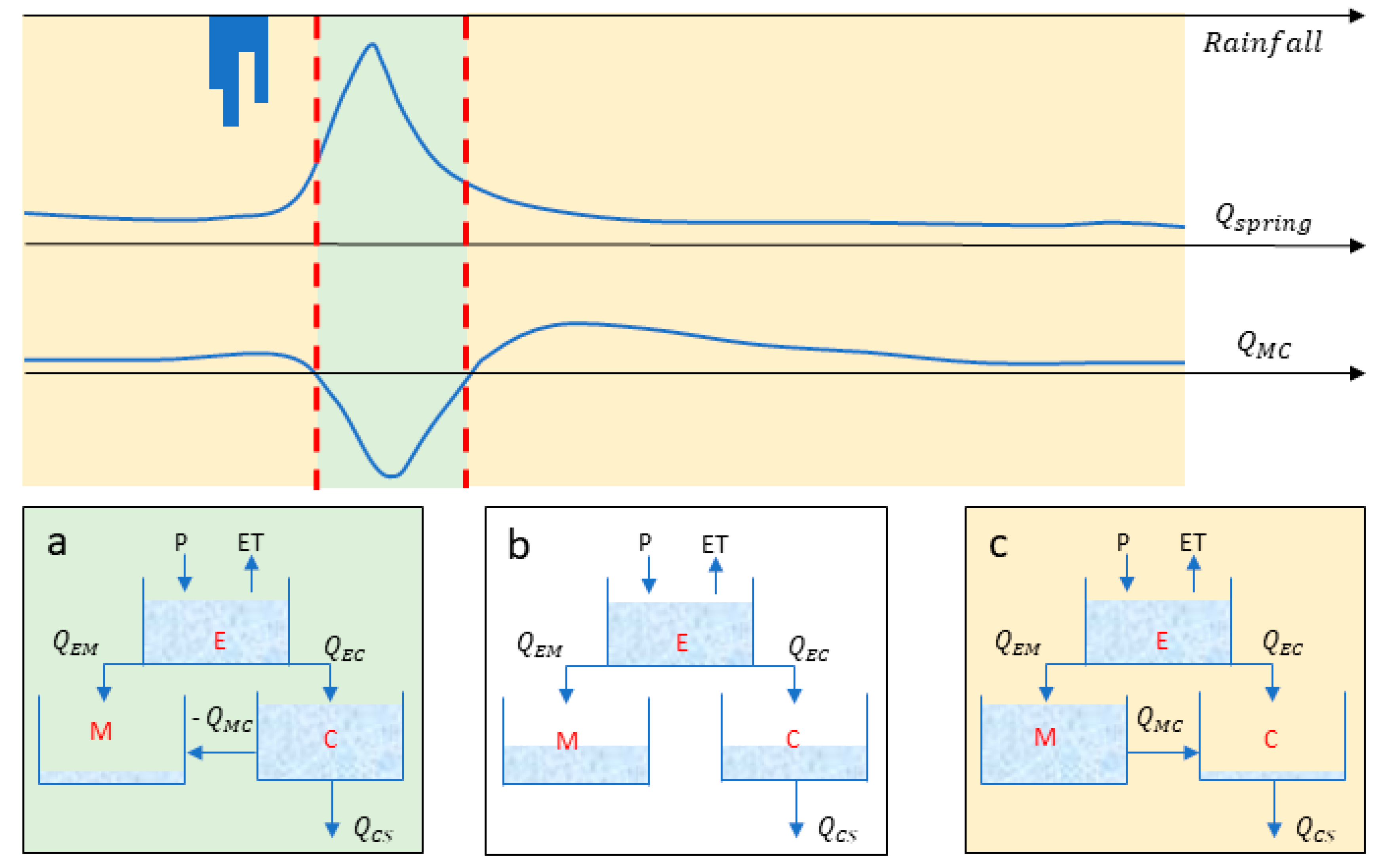
Top: synthetic time series of rainfall, spring discharge (Qspring) and matrix-conduit flow dynamics (QMC); Bottom: Structure of the reservoir model: epikarst (E), matrix (M) and conduit (C) are inter-connected from the top to the bottom of the structure. QMC corresponds to the flow from reservoir M to reservoir C and depends on the difference between water levels in M and C. The model is considered on several time steps: (a) the water level is higher in reservoir C, so QMC < 0; (b) the water level in reservoirs C and M are equal, so QMC = 0 and (c) the water level is higher in M so QMC > 0.
Figure 2.
Top: synthetic time series of rainfall, spring discharge (Qspring) and matrix-conduit flow dynamics (QMC); Bottom: Structure of the reservoir model: epikarst (E), matrix (M) and conduit (C) are inter-connected from the top to the bottom of the structure. QMC corresponds to the flow from reservoir M to reservoir C and depends on the difference between water levels in M and C. The model is considered on several time steps: (a) the water level is higher in reservoir C, so QMC < 0; (b) the water level in reservoirs C and M are equal, so QMC = 0 and (c) the water level is higher in M so QMC > 0.

Figure 3.
Example of event base time series for KarstMod model on Aliou watershed on the hourly sampling rate: (a) Rainfall time series with observed and simulated discharge; (b) water level in KarstMod reservoirs E, M and C and (c) fluxes between reservoir M and C. When QMC > 0, the flow goes from reservoir M to C, otherwise the flow goes from reservoir C to M.

Figure 4.
MASH of the daily rainfall (w = 30 days, Y = 15 years). The dates correspond to the starting year, noted Ys, for shifting horizon average, so the corresponding shifting horizon period is from the starting year Ys to Ys + 15 years. Due to the 15 years moving average window, the abscissa finished in 2003.

Figure 5.
MASH of the estimated water volume in the reservoir M (w = 30 days, Y = 15 years).

Figure 6.
Contribution of the exchange between reservoir M and reservoir C to the total discharge on the annual scale (left) and the monthly scale (right).
Figure 6.
Contribution of the exchange between reservoir M and reservoir C to the total discharge on the annual scale (left) and the monthly scale (right).


Table 1.
Warm-up, calibration and validation periods for KarstMod models.
| [24 h] | [1 h] | |||||
|---|---|---|---|---|---|---|
| Period | Warm-Up | Calibration | Validation | Warm-Up | Calibration | Validation |
| from | 1 January 1968 | 1 October1970 | 1 October 1980 | 1 October 2009 | 1 October 2010 | 1 October 2012 |
| to | 30 September 1970 | 30 September 1980 | 31 December 2016 | 30 September 2010 | 30 September 2012 | 31 May 2017 |
Table 2.
Calibration values of the model parameters for Aliou and Baget watersheds.
| Parameter | Calibration [24 h] | Calibration [1 h] | ||
|---|---|---|---|---|
| Aliou | RA | Recharge area | 14.8 km2 | 14.2 km2 |
| kEM | Recession coefficient from E to M | 6.10 × 10⁻³ mm/day | 1.11 × 10⁻⁴ mm/h | |
| kEC | Recession coefficient from E to C | 9.83 × 10⁻³ mm/day | 2.69 × 10⁻³ mm/h | |
| kCS | Recession coefficient from C to S | 2.36 × 10⁻³ mm/day | 1.80 × 10⁻⁴ mm/h | |
| kMC | Recession coefficient from M to C | 3.17 × 10⁻¹ mm/day | 2.41 × 10⁻² mm/h | |
| Baget | RA | Recharge area | 15.8 km2 | 13.1 km2 |
| kEM | Recession coefficient from E to M | 3.36 × 10⁻³ mm/day | 2.09 × 10⁻⁴ mm/h | |
| kEC | Recession coefficient from E to C | 2.71 × 10⁻³ mm/day | 4.35 × 10⁻⁴ mm/h | |
| kCS | Recession coefficient from C to S | 1.21 × 10⁻³ mm/day | 7.21 × 10⁻⁴ mm/h | |
| kMC | Recession coefficient from M to C | 7.03 × 10⁻² mm/day | 1.25 × 10⁻¹ mm/h |
Table 3.
Model performances for calibration and validation periods for daily and hourly KarstMod models (NSE: Nash Sutcliff Efficiency, BE: Balance Error and KGE: Kling Gupta Efficiency).
Table 3.
Model performances for calibration and validation periods for daily and hourly KarstMod models (NSE: Nash Sutcliff Efficiency, BE: Balance Error and KGE: Kling Gupta Efficiency).
| [24 h] | [1 h] | ||||
|---|---|---|---|---|---|
| Periods | Calibration | Validation | Calibration | Validation | |
| (1970–1980) | (1980–2016) | (2010–2012) | (2012–2017) | ||
| Aliou | NSE | 0.53 | 0.51 | 0.63 | 0.5 |
| BE | 0.88 | 0.97 | 0.99 | 0.91 | |
| KGE | 0.58 | 0.51 | 0.67 | 0.54 | |
| Baget | NSE | 0.59 | 0.52 | 0.56 | 0.47 |
| BE | 0.94 | 0.89 | 0.98 | 0.77 | |
| KGE | 0.61 | 0.52 | 0.64 | 0.44 | |
© 2019 by the authors. Licensee MDPI, Basel, Switzerland. This article is an open access article distributed under the terms and conditions of the Creative Commons Attribution (CC BY) license (http://creativecommons.org/licenses/by/4.0/).
Share and Cite
MDPI and ACS Style
Sivelle, V.; Labat, D.; Mazzilli, N.; Massei, N.; Jourde, H. Dynamics of the Flow Exchanges between Matrix and Conduits in Karstified Watersheds at Multiple Temporal Scales. Water 2019, 11, 569. https://doi.org/10.3390/w11030569
AMA Style
Sivelle V, Labat D, Mazzilli N, Massei N, Jourde H. Dynamics of the Flow Exchanges between Matrix and Conduits in Karstified Watersheds at Multiple Temporal Scales. Water. 2019; 11(3):569. https://doi.org/10.3390/w11030569
Chicago/Turabian StyleSivelle, Vianney, David Labat, Naomi Mazzilli, Nicolas Massei, and Hervé Jourde. 2019. "Dynamics of the Flow Exchanges between Matrix and Conduits in Karstified Watersheds at Multiple Temporal Scales" Water 11, no. 3: 569. https://doi.org/10.3390/w11030569
Note that from the first issue of 2016, this journal uses article numbers instead of page numbers. See further details here.