Spatiotemporal Dynamics of Submerged Aquatic Vegetation in a Deep Lake from Sentinel-2 Data
by
 , ,
, ,
Nicola Ghirardi
1, 
Rossano Bolpagni
1,2,*,
Mariano Bresciani
1,
Giulia Valerio
3,
Marco Pilotti
3 and
Claudia Giardino
1 1
Institute for Electromagnetic Sensing of the Environment, Consiglio Nazionale delle Ricerche, via Bassini 15, 20133 Milan, Italy
2
Department of Chemistry, Life Sciences and Environmental Sustainability, University of Parma, Parco Area delle Scienze 11/A, 43124 Parma, Italy
3
DICATAM, Università degli Studi di Brescia, via Branze 43, 25123 Brescia, Italy
*
Author to whom correspondence should be addressed.
Water 2019, 11(3), 563; https://doi.org/10.3390/w11030563
Submission received: 21 January 2019
/
Revised: 11 March 2019
/
Accepted: 14 March 2019
/
Published: 18 March 2019
(This article belongs to the Special Issue Application of Remote Sensing and GIS in Aquatic Ecosystems)
Abstract
:We mapped the extent of submerged aquatic vegetation (SAV) of Lake Iseo (Northern Italy, over the 2015–2017 period based on satellite data (Sentinel 2 A-B) and in-situ measurements; the objective was to investigate its spatiotemporal variability. We focused on the southern sector of the lake, the location of the shallowest littorals and the most developed macrophyte communities, mainly dominated by Vallisneria spiralis and Najas marina. The method made use of both in-situ measurements and satellite data (22 Sentinel 2 A-B images) that were atmospherically corrected with 6SV code and processed with the BOMBER (Bio-Optical Model-Based tool for Estimating water quality and bottom properties from Remote sensing images). This modeling system was used to estimate the different substrate coverage (bare sediment, dense stands of macrophytes with high albedo, and sparse stand of macrophytes with low albedo). The presented results substantiate the existence of striking inter- and intra-annual variations in the spatial-cover patterns of SAV. Intense uprooting phenomena were also detected, mainly affecting V. spiralis, a species generally considered a highly plastic pioneer taxon. In this context, remote sensing emerges as a very reliable tool for mapping SAV with satisfactory accuracy by offering new perspectives for expanding our comprehension of lacustrine macrophyte dynamics and overcoming some limitations associated with traditional field surveys.
1. Introduction
Investigating the dynamics of lacustrine submerged aquatic vegetation (SAV) is a challenging topic due to the complex processes involved in driving SAV’s responses to internal and external determinants [1,2]. Macrophytes act as ecosystem engineers that are able to deeply regulate the colonized habitats [3,4]. However, they are also extremely sensitive to human perturbations, especially to eutrophication—a human-induced increase in nutrient availability that favors the growth and reproduction of algae or invasive plant species, thus reducing SAV’s health, performance, and diversity [5].
Most of the aquatic ecosystems worldwide have been affected by dramatic perturbations over the last two centuries, and macrophytes are among the most threatened biotic component [6,7]. Furthermore, an increasing awareness of the role of global warming in driving macrophyte growth patterns has emerged in the last decades. Strong evidence suggests the importance of local climate variability in modulating the state of clear-water [8,9,10] and the role of periods of frost in modulating the competition dynamics of macrophytes in shallow lakes [11].
Generally, it is critical to be able to disentangle the bijective interactions of natural and human determinants in influencing macrophyte distribution and dominance [12]. Several works have been done to investigate the contribution of human impacts on such changes [13,14,15,16,17]. On the contrary, only few studies have investigated non-nutrient drivers of macrophyte growth and distribution [18,19] or focused on their natural successional patterns [11,20]. Moreover, research interests have largely focused on alteration processes of SAV instead of analyzing the intrinsic dynamics.
The possibility of investigating SAV phenology can open new ways for a better comprehension of the hidden processes that influence seasonal dynamics of SAV [21,22]. Bolpagni et al. (2016) [1] showed that the SAV dynamics can change quickly in a series of volcanic lakes of Central Italy. In particular, a significant reduction in the maximum growing depth of macrophytes, especially within the deepest stonewort communities (below 5 m), was observed over a three year period, despite the absence of evident external perturbation events, either of climatic or anthropogenic origin (e.g., human derived water variations or physical and chemical water conditions).
Remote sensing has been used for many years for mapping of bottom cover types and benthic communities (e.g., mud, sand-mud mixture, coral sands, coral reefs, seagrass, macrophytes). In particular, recent reviews of the state of the art were published by Malthus (2017) [23] and Hedley et al. (2018) [24] for aquatic macrophytes and for coral reefs, respectively. Both reviews recognized that multispectral sensors are suitable for large-scale and long-term monitoring of lacustrine SAV. In particular, even if Landsat offers the clear advantage for long-term retrospective studies [25], Sentinel-2 allows for improving the spatial and temporal resolutions of the analysis. In fact, Sentinel-2 data offer additional bands in the visible (VIS) and near-infrared (NIR) region, higher radiometric sensitivity, signal-to-noise ratios, and the spatial resolution of up to 10 m, allowing more detailed studies on SAV [26,27]. Common methods applied to satellite imagery include the inversion of physically based models [28] based on former studies by Lee et al. (1999, 2001) [29,30]. Several authors extended the method [31] to a wide range of applications, including SAV mapping from Sentinel-2 [32,33,34,35].
In this context, the main objectives of this paper are to map the distribution of SAV in a deep lake (Lake Iseo; Northern Italy) and to quantify SAV’s spatiotemporal variations using Sentinel-2 data over a three years period (2015–2017). Specifically, we focus our attention on the bathymetric layer between 0 and 10 m of depth that is the colonization horizon of macrophytes in the lake under investigation. We also examine the effect of coastal distance on the spatial arrangement of SAV. Our main expectations are that significant variations in terms of colonized areas have characterized SAV across years and depths.
2. Materials and Methods
2.1. Study Area
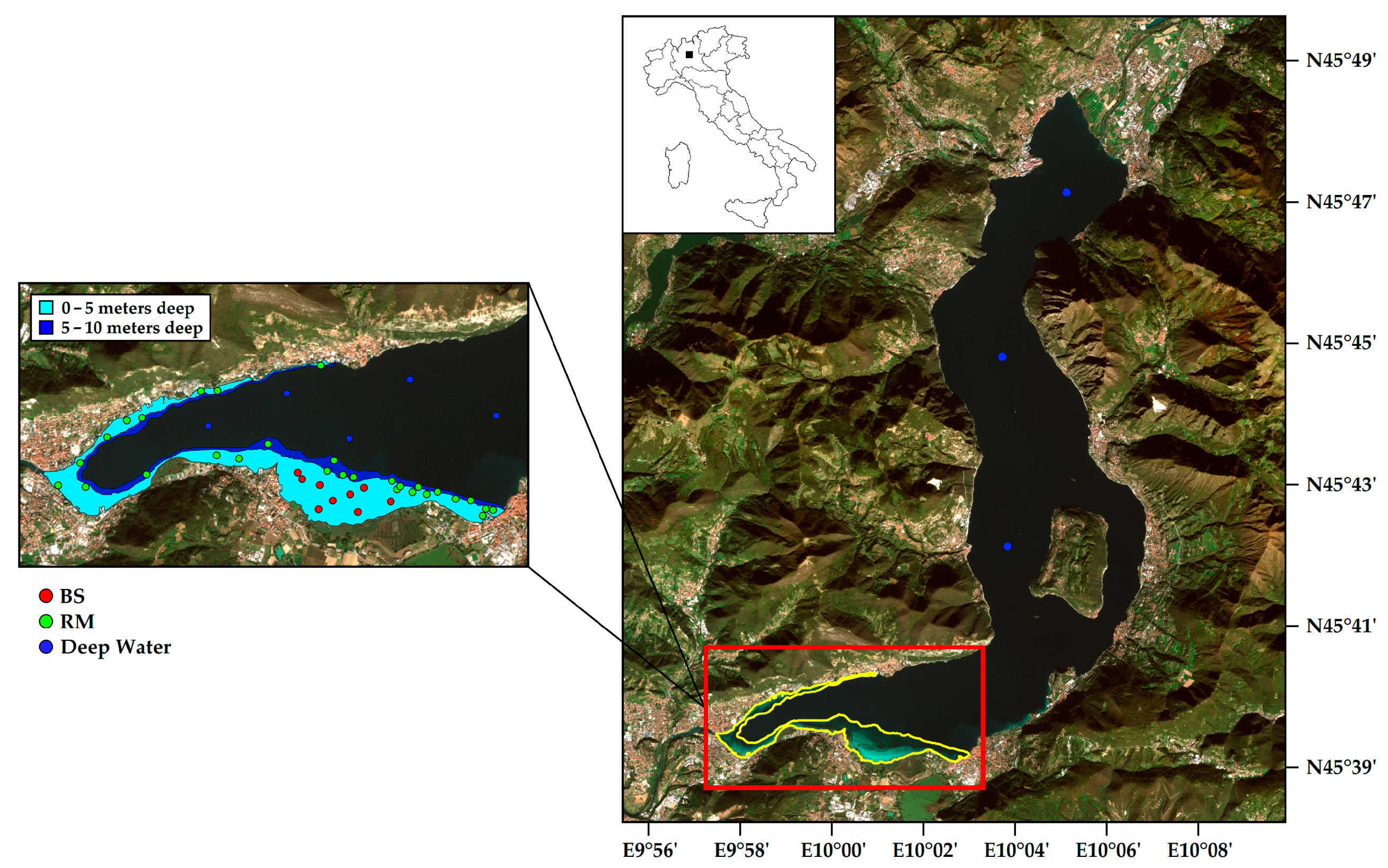
Lake Iseo is a deep Italian pre-alpine lake with a maximum depth of 258 m and a mean depth of 124 m. This lake is characterized by a volume of 7.6 km3, a surface area of 61.8 km2, and a theoretical renewal time of the lake of 4.5 years [36]. However, due to its thermal stratification, the actual time T37 (renewal time 37)—namely, when the 37% of the original water is still present within the lake—is 60% longer and will keep growing with the reinforced thermal stratification [36] that will be a likely consequence of climate change. It is situated in Northern Italy (Lombardy Region) and hosts Montisola—the largest and highest island of sub-alpine lakes. According to Hutchinson (1957) [37], Lake Iseo should be considered as “warm monomictic” since its water temperature never drops below 4 °C. Nevertheless, water full circulation is usually incomplete and occurs only in conjunction with very cold and windy winters (over the last twenty years, only in 2005 and 2006). Consequently, Lake Iseo can be considered as “oligomictic” [38,39,40,41,42,43]. In recent decades, this has led to a densimetric stratification of the mass of water, which is typical of “meromictic lakes” and is associated with a marked deterioration of the trophic state of the lake, a phenomenon that is particularly relevant for the deep layers. Hence, total phosphorus (TP) concentrations increased from about 60 (1992) to 90–100 μg P L−1 (2016) in the hypolimnion (15–258 m) [43]. The Secchi disk values never exceed 4.5 m of depth, suggesting a local maximum growing depth of 9–10 m for SAV [44]. Accordingly, we limited our inspection to 10 m of depth, focusing on the southern part of the lake (Figure 1), a strongly human-impacted sector where gentle slopes and shallow waters enable the substrates to be intensely colonized by SAV, as verified by ARPA Lombardia (Regional Agency for Environmental Protection of Lombardy Region; [44]). Within the 0–10 m depth range, the analyses were performed by splitting the depths into two bottom depth layers corresponding to 0–5 (282.5 ha) and 5–10 (71.5 ha) m deep (Figure 1). For 2017 and over the same depth range, we also evaluated the spatial variability of SAV as a function of the distance from the coastline. To this aim, we defined seven distance classes: 10–25 m, 26–50 m, 51–100 m, 101–200 m, 201–350 m, 351–600 m, and >600 m, that were chosen in order to have comparable littoral belts in terms of surface area. Bathymetry and coastal distance are strongly dependent on each other, but the spatial scale of analysis could influence their relationship. Therefore, we decided to investigate their role as spatiotemporal drivers of SAV separately for distance classes.
SAV is mainly dominated by Vallisneria spiralis and Najas marina, able to form dense and very uniform stands with cover values up to 95–100%, with a minor contribution of Lagarosiphon major, Ceratophyllum demersum, and Myriophyllum spicatum (with cover values in the range 5 to 10%). The studied SAV’s biomass ranged from a few grams DW (dry weight) per m2 (bare to sparse cover) to ~0.5 kg DW m−2 (dense cover) (Bolpagni, unpublished data), confirming the meso-eutrophic condition of the lake [43].
2.2. Image Processing
Sentinel-2 images were used to evaluate the spatiotemporal dynamics of SAV in the southern sector of the Lake Iseo. The two Sentinel-2 twin satellites (S2A and S2B) carry on board the MultiSpectral Instrument (MSI) optical sensor, which acquires images in 13 bands (spectral region between 442 and 2201 nm) with a spatial resolution of 10, 20, and 60 m (depending on the spectral band). For this study, the first 7 bands of the VIS–NIR region were used, all reprocessed at the spatial resolution of 10 m. A total of 17 cloud free images available between 2015 and 2017 were analyzed. Nine of them were used to investigate the intra-annual dynamics (from late March to late October). The remaining eight, four in 2015 (from early April to late September) and the other four in 2016 (from late March to mid-October), were used to investigate the inter-annual dynamics.
The 17 Sentinel-2A and -2B TOA (top of atmosphere) radiances were computed from the MSI level2 TOA reflectance images (downloaded from Copernicus Open Access Hub) by using the SNAP tool ReflectanceToRadianceOp. TOA radiance products were atmospherically corrected with the Second Simulation of the Satellite Signal in the Solar Spectrum code-vector version (6SV) [45,46]. The code was parametrized with aerosol optical thickness (AOT) and aerosol microphysical properties information at the time of imagery acquisition and collected from a nearby AERONET station [47]. The 6SV-derive reflectance was converted in remote sensing reflectance (RRS) dividing by pi. The reflectance products obtained were previously validated in Bresciani et al. (2018) [48].
RRS products were then used as the input of a non-linear optimization algorithm called BOMBER (Bio-Optical Model-Based tool for Estimating water quality and bottom properties from Remote sensing images) [49] for estimating the substrate coverage. The parameterization of the bio-optical model implemented in BOMBER was based on a comprehensive in situ dataset dedicated to sub-alpine lakes [48,50,51]. With respect to Lee et al. [29], who described bottom albedo ρ (λ) as the albedo value at a reference wavelength, in this study, the ρ (λ) was expressed as a linear combination of three substrates with different albedo values. The BOMBER bio-optical modeling system was applied to reflectance products in shallow water mode. For each image, BOMBER was only run for the pixels corresponding up to 10 m of bottom depth.
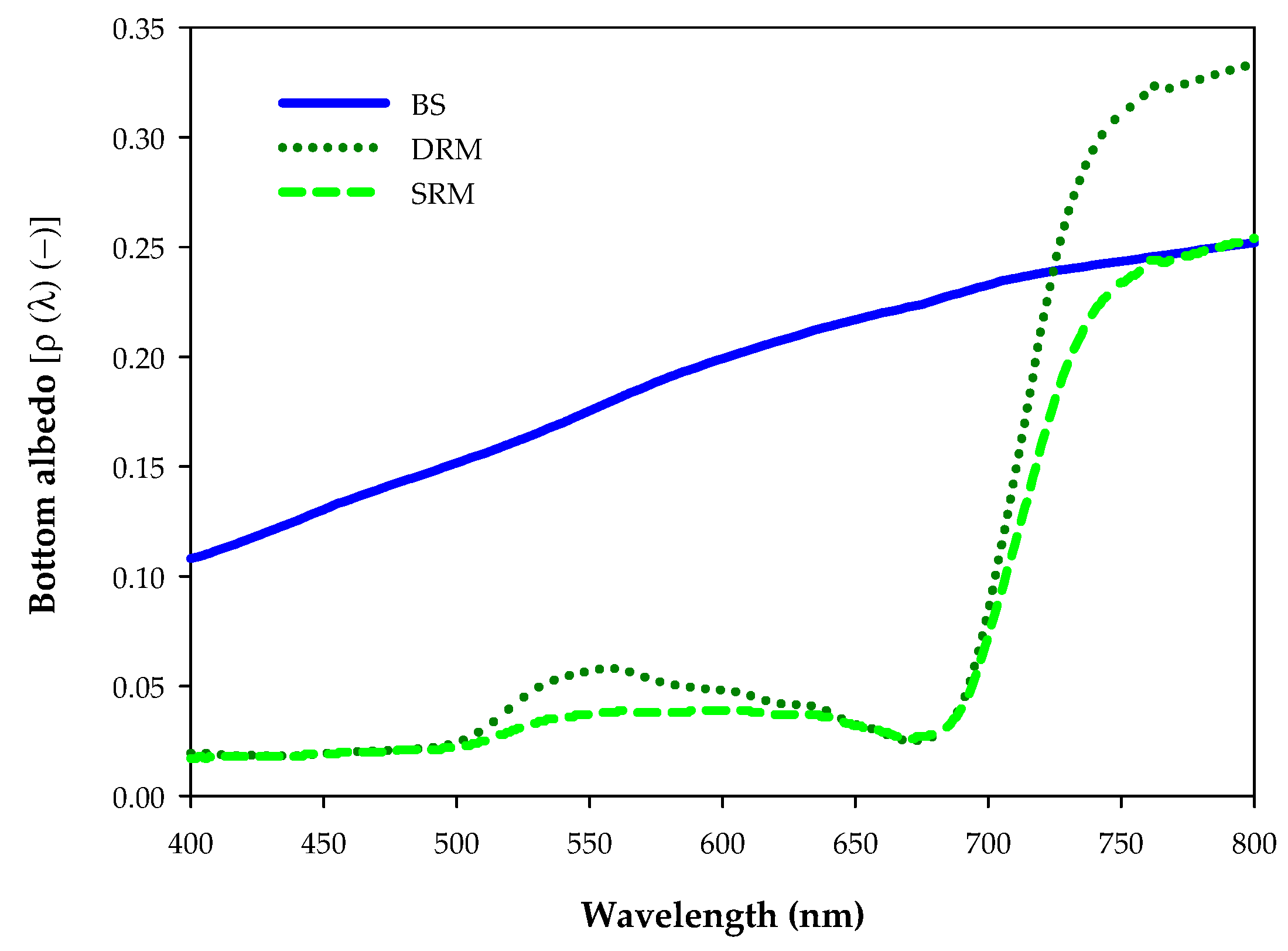
The three spectra (Figure 2) were the average value of measured reflectance spectra of different bottom cover types present in the study area: BS = bare sediment; DRM = dense stands of rooted macrophytes (with high albedo), and SRM = sparse stands of rooted macrophytes (with low albedo). For the comparison among years, the two SAV’s classes obtained by BOMBER (DRM and SRM) were summed in order to obtain aggregated values (expressed as RM = DRM + SRM) in order to better understand SAV’s dynamics.
In addition to the three above-introduced bottom cover types, it was possible to identify a fourth one for the floating stands of uprooted macrophytes (mainly consisting of detached individuals of V. spiralis). Floating patches were identified by calculating the ratio between the b6 band (~740 nm) and the b3 band (~560 nm) of the atmospherically corrected reflectance. Under standard conditions, water absorbs in the infrared wavelength; therefore, in the absence of floating macrophytes, the b6 band is expected to be smaller than the b3 band. Consequently, when b6 > b3, we expected the presence of floating macrophyte stands.
The remote sensing products were validated with the acquisition of in situ records collected on 8 July 2016, 26–27 September 2016, and 26–31 July 2017. A total of 47 field points were available for building a confusion matrix and hence for computing the satellite-products accuracy from an independent dataset (Figure 1). For each plot, we also took in situ georeferenced points with notes on macrophytes species. Validation points were selected randomly in the range 0–10 m of depth, taking into account the data collected by ARPA Lombardia, and were equally distributed between the two depth layers under investigation (0–5 and 5–10 m depth). Presence and absence SAV’s records were used to validate the outputs of BOMBER bio-optical modeling, verifying its ability to discriminate across bottom cover classes. These data were used to generate a confusion matrix to evaluate the class combination for each bottom cover class in analysis [BS; RM = submerged rooted macrophytes, obtained summing dense (DRM), and sparse (SRM) macrophyte-covered areas)]. An additional class referring to deep water (for depths greater than 10 m) was also introduced to refine remote sensing products.
3. Results
3.1. Validation Results
The confusion matrix confirms that all the classes were recognized well with an overall accuracy of 93.6% (Table 1). A slight high misidentification was found for deep water (88.9%), while the two classes of SAV (here considered as RM) and bare sediments were mapped with high accuracy (>93.5% and 100.0%, respectively).
3.2. Intra-Annual (2017) Spatiotemporal Dynamics of SAV and Bare Sediment
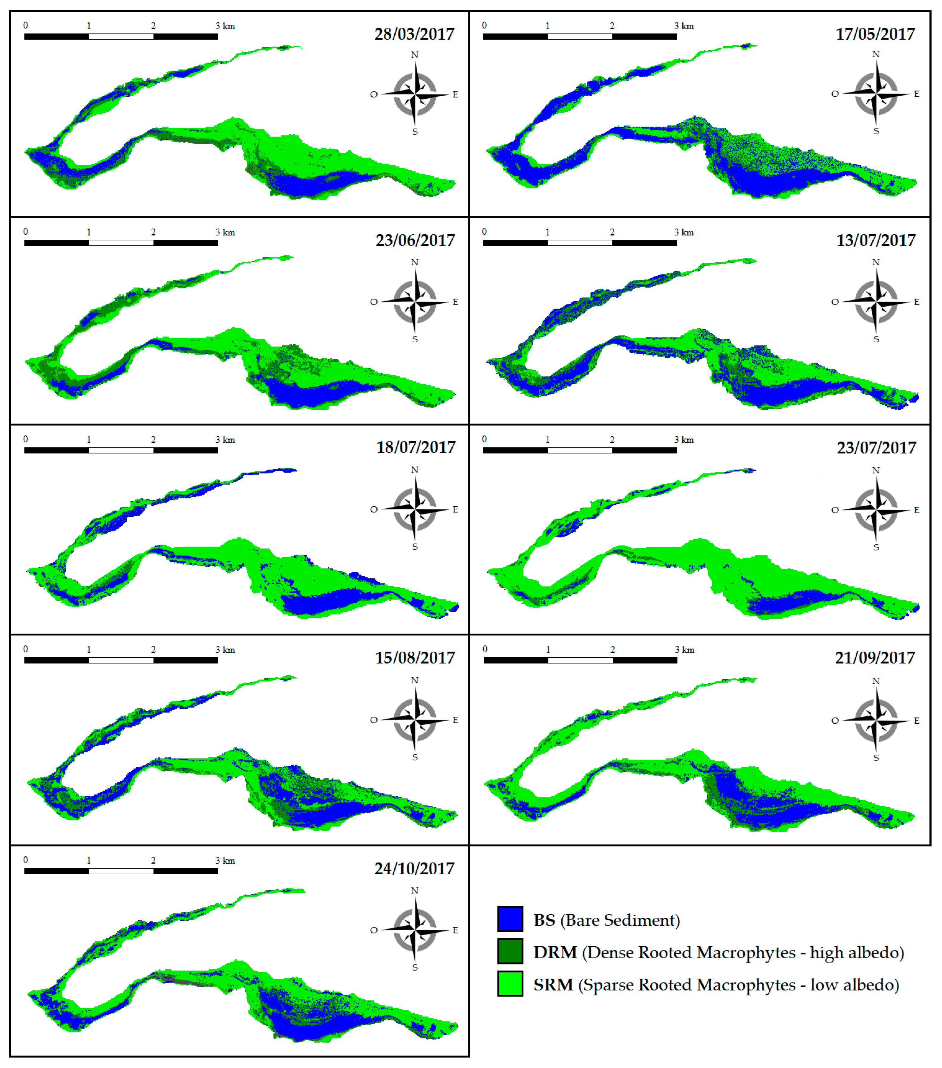
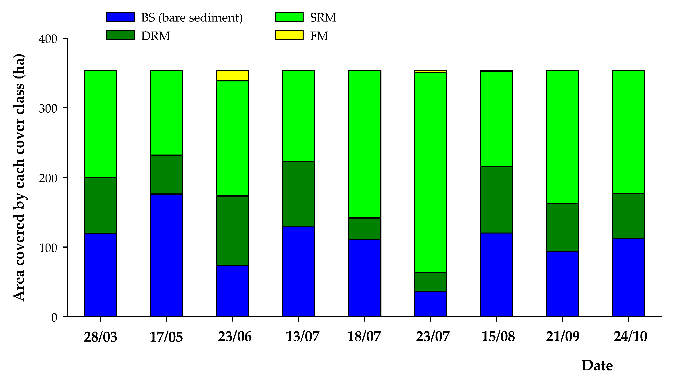
During the 2017 growing season (from late March to late October), the southern part of Lake Iseo under consideration (for a total surface of 354 ha) turned out to be largely colonized by SAV (Figure 3, Figure 4 and Figure 5). Overall, SAV’s representativeness—expressed as RM—varied in the range of 51–89% with a mean value of 70%. In general, the RM increased its cover rates along with growing season until reaching the peak in late July and then decreased during the autumn period (with values in the range of 64–73%). However, the lowest cover rate was measured in mid-May. Nonetheless, the class BS was locally well represented as well, with cover percentages varying from a minimum of 11% to a maximum of 49%.
Focusing on the two different macrophyte classes in analysis, the percentage of coverage of DRM was constantly lower than that of SRM. In particular, the percentage of coverage of DRM remained more or less stable around values of 15–29% except after mid-July, where it fell to 9–10%. Conversely, the percentage of coverage of SRM varied instead between 34% and 81% with a mean value of 49%. Therefore, the average difference between the percentages of coverage of these two bottom cover classes was 30% with a minimum difference of 5% and a maximum difference of 71% (Figure 3). In Figure 5, we report the coverage variations in ha.
3.3. Spatiotemporal SAV Dynamics across Years (2015–2017)
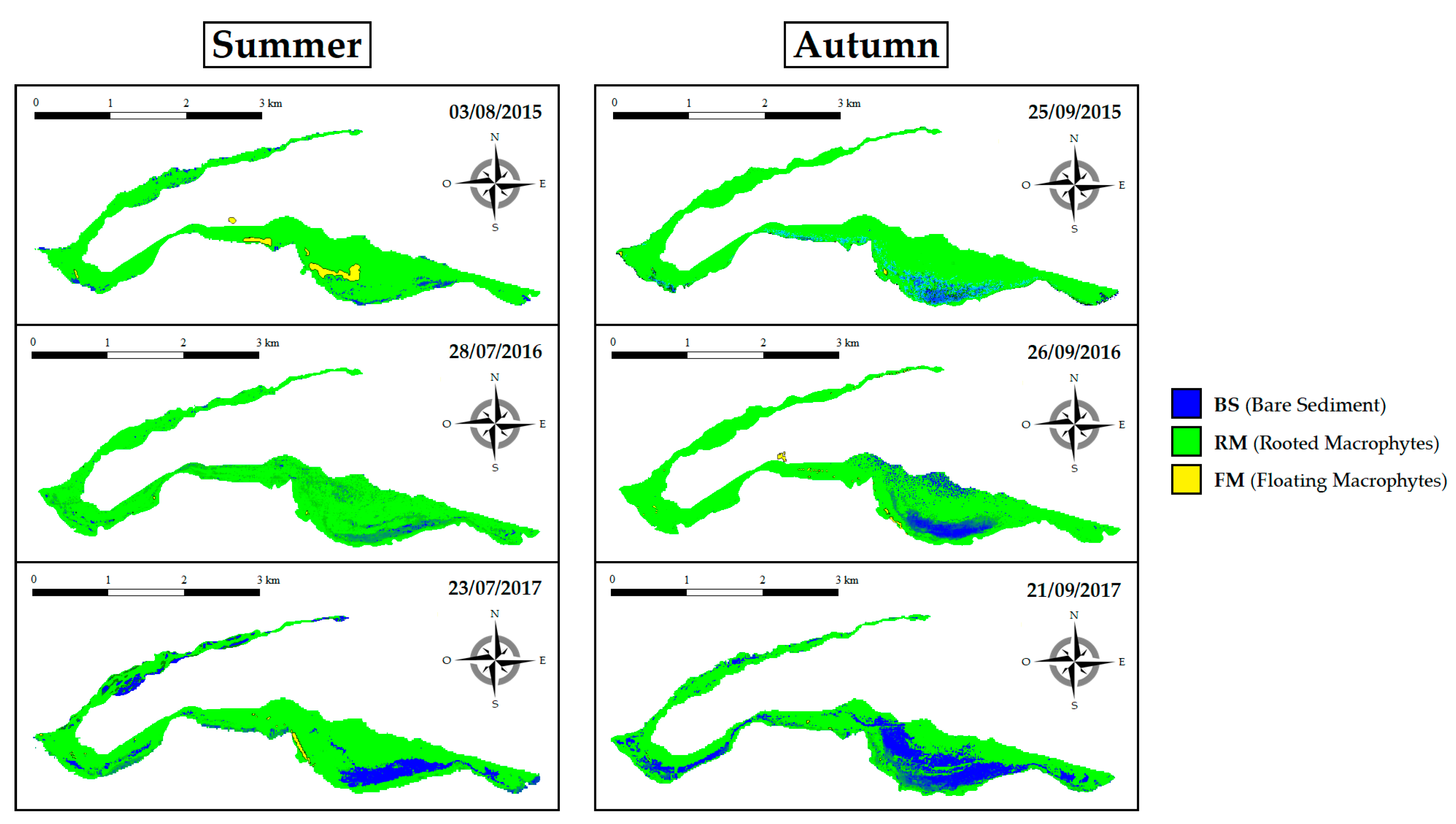
Comparing data from mid-summer and early autumn, the percentage cover of RM turned out—as expected—to be higher during summer than during autumn periods for all the years under consideration (Figure 6). In particular, in 2015, RM’s coverage was 94% in summer and 91% in autumn. In 2016, it was 94% in summer and 91% in autumn. Finally, in 2017, it was 89% in summer and 73% in autumn. During summer, RM’s coverage underwent slight fluctuations over the three years under analysis equal to the 5% moving from the highest (94%) to the lowest rate (89%). In contrast, in the autumn period, the decrease in cover percentage was much more pronounced and equal to 18% comparing the highest (91%) with the lowest percentage (73%). Additionally, the inter-annual comparisons allowed us to quantify the SAV’s uprooting phenomenon. In 2015, this phenomenon peaked twice, covering an area of about 28 ha on 7 April (data was not shown) and 10 ha on 3 August (Figure 6). In 2017, the largest coverage of floating macrophytes was recorded on 23 June, covering an area of 15 ha. Conversely, for 2016, the uprooting events were extremely limited.
3.4. Role of Bathymetry and Coastal Distance in SAV Dynamics
Bathymetry and the distance from the lake coastline seemed to have relevant roles in driving the inter-annual cover rate pattern of RM and BS (Figure 7). Considering SAV’s dynamics across years in terms of bathymetric layers, higher RM coverage values (when normalized with the layer area) were detected for the shallow layer (i.e., 0–5 m) during the seasons (in the range of 46.1–65.2%) compared to the deepest one (5–10 m; 31.7–38.0%). Equally, BS coverage values tended to be largely higher in the shallower versus deeper layers, with values in the range of 1.4–23.2% and 0.0–5.8%, respectively. For RM, a progressive decrease in coverage values was observed in the shallower layer for both periods analyzed (i.e., peak of season and senescence); on the other hand, minor variations were detected for the deeper layer. For the summer period, the overall decrease in RM coverage was around 26 ha from 2015 to 2017, whereas for the autumn period, this decrease turned out to be 78 ha. With respect to BS, the observed trends mirrored RM coverage values. In fact, in the shallower layer, BS’ coverage increased from 2015 to 2017 both in the summer and in autumn period. On the other hand, in the deeper layer, BS’ values remained constant over the monitored years. In particular, for the shallower layer, the highest increase rate was recorded in autumn (+78 ha), whereas a smaller increase was observed for the summer period (+27 ha).
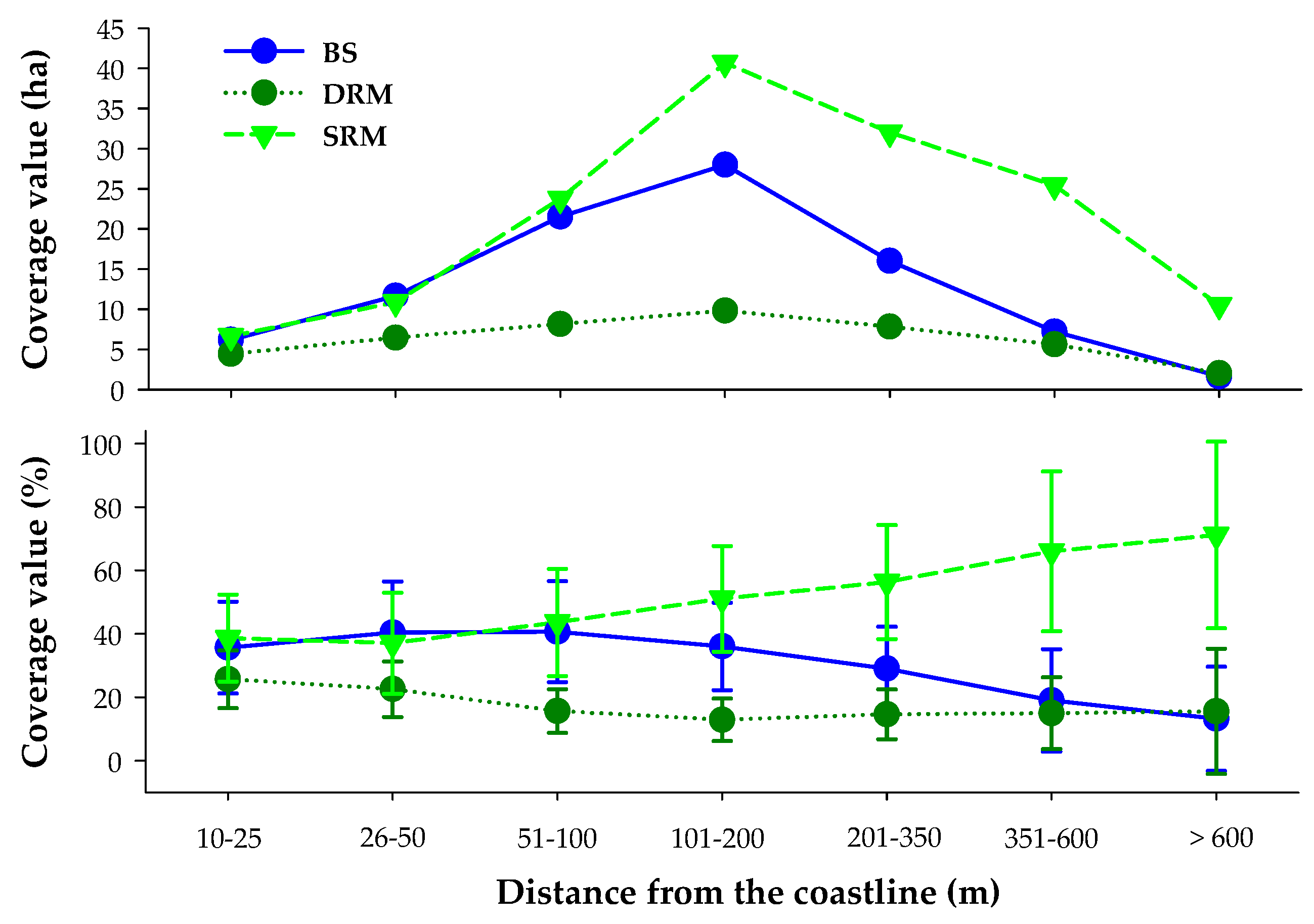
Focusing on the distance from the lake coastline, the average cover values calculated for each class (obtained considering only the 2017 scenes) revealed SRM as the dominant bottom cover class, especially starting from 100 m from the coastline with highest coverage reaching up to 70% beyond 600 m (Figure 7). The DRM class was the least represented with coverages almost constant except in front of the coastline, as in the first 50 m from the coast, the percentage of coverage exceeded 20%. Finally, BS class was well represented in the first 100 m from the coastline (with a percentage of coverage around 40%). At longer distances, a progressive decrease was observed for increasing distance towards the pelagic waters (Figure 7).
4. Discussion
During the period under investigation (2015–2017), the study area was affected by relevant variations in the spatial patterns of SAV, locally represented by submerged beds largely dominated by V. spiralis and N. marina. These two species are able to colonize large sectors of the littorals, creating dense stands with cover values in the range of 70–100%, and with the presence of very few companion species (mainly L. major and M. spicatum).
The results show that SAV coverage significantly changes across seasons and years in Lake Iseo, as expected for deep lakes [52] and also reported by Bolpagni et al. (2016) [1]. In this context, remote sensing seems a viable tool to detect and investigate very rapid successional processes (i.e., inter and intra-annual variation), as well as to quantify the surface areas involved—processes that would, instead, be impossible to adequately evaluate using classical approaches (e.g., by macrophyte survey along transects as imposed by the Water Framework Directive implementation) [53,54]. This stresses the pivotal contribution that remote sensing can play in the analysis of underlying processes of aquatic ecosystems in the coming years.
Overall, a decrease of 67 ha of SAV was recorded during the autumn period over the three analyzed years, equal to 18% of the entire area investigated (of ~354 ha, which represents more than 50% of the entire lake littorals potentially colonized by SAV). Focusing on 2017 data, during the first growth phase until early July, SAV was characterized by an accentuated variability with phases of expansion and contraction, then stabilizing and rapidly reaching the peak of growth in late July (with cover percentage values up to ~90.0%).
Bathymetry, as well as the distance from the coastline, appeared to have relevant roles in driving the observed inter- and intra-annual pattern of SAV and bare sediment, reaffirming the existence of a clear spatial determination of macrophytes distribution, with the highest cover rates measured in the upper layer (0–5 m). This is especially true for SAV, both in relative and absolute terms. Hence, rooted macrophytes exhibited a progressive decrease over the 2015–2017 period, especially in the autumn period (from 253.7 to 228.0 ha and from 263.6 to 185.6 ha for summer and autumn period, respectively). On the contrary, bare sediments cover values exhibited inverse trends. Conversely, no clear trends were recognized for either of the bottom cover classes in the lower layer (5–10 m). Accordingly, an increase in sparse SAV stands with the progressive increase in coastline distance was also observed. These two factors are strictly under the control of the water level variations, which can further accentuate the bathymetry effect on SAV dynamics, as recently confirmed by Ławniczak-Malińska et al. [55]. In the period under investigation, the lake water level fluctuations varied significantly across years, with mean values in the range 27.7 (2015) and 57.2 cm (2016) above the hydrometric reference level (www.laghi.net). However, the maximum differences between hydrometric levels never exceeded 30 cm, suggesting a limited effect on the observed SAV trajectories.
Additionally, these results are also in line with the generally acknowledged detrimental effects of water eutrophication to SAV via increased shading modulated by phytoplankton and periphyton along with increasing in water depths [56,57]. Eutrophication supports regime shifts, intensifying rapid turnover of dominant macrophytes, which can determine significant variations in SAV patterns, as observed in Lake Iseo. In this context, future investigations will be needed to better understand the recorded SAV’s behavior, with attempts to couple satellite images with physical and chemical water conditions and determinants. Nevertheless, in the case of deep lakes, phytoplankton tends to occupy the entire euphotic zone (up to ~20 m of depth for Lake Iseo), privileging the pelagic sectors (15–19 m) [38]. Along the lake littorals, the phytoplankton chlorophyll-a concentrations do not exceed 8–10 μg L−1, suggesting a minor role in driving the SAV dynamics [38].
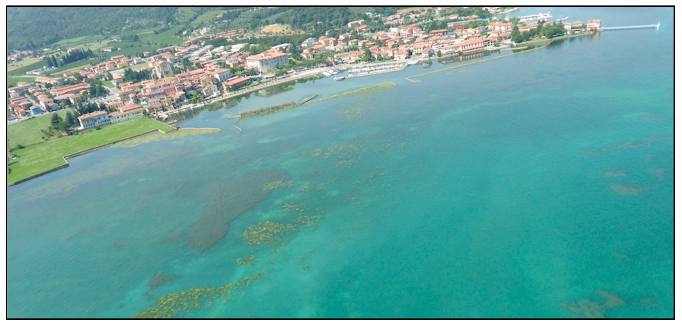
Additionally, our data have also highlighted the presence of the peculiar phenomenon of the SAV uprooting (see also Figure 4 and Figure 5), mainly due to the detaching of submerged stands of V. spiralis. Aquatic plant uprooting events are expected to be related to an excessive organic matter accumulation in sediments. This condition is able to stimulate a reduction in sediments’ cohesion, which consequently leads to an increased risk of macrophyte uprooting [58]. However, these phenomena are normally diffused in oligo to meso-trophic water bodies and affect macrophytes characterized by high levels of sensitivity to the organic enrichment of sediments (i.e., isoetids; [59] and references therein). Here, the fact that the uprooting was detected for V. spiralis, an engineering species that creates a dense root system able to fix sediments, shows that very intense degenerative processes in superficial sediments are in progress.
It is interesting to observe that the investigated area is located just in front of an active combined sewer weir (CSW) whose overflows significantly contribute to the nutrient pollution of this littoral area [60]. The future comparative analysis of the CSW overflows and of the SAV extension will certainly provide important insights to the comprehension of the SAV dynamics. Further investigations must be done in order to better evaluate these processes and to counteract the loss of SAV. These processes, in fact, do not only determine local effects; they also influence downstream ecosystems, but in particular, exacerbate the management costs of the entire network of irrigation channels that is fed by Lake Iseo.
5. Conclusions
The use of Sentinel-2 data offered the possibility of mapping SAV and floating aquatic vegetation for supporting ecosystems monitoring in the most important shallow water zone of Lake Iseo. An approach based on physics-based model inversion was used to classify the bottom cover classes as bare sand and SAV, the latter according to two levels of colonization coverage density (dense and sparse) up to 10 m depth. These products enable us to move forward to the assessment of SAV ecosystems and might permit further investigation to improve studies on aquatic vegetation phenology, such as that recently demonstrated by Pinardi et al. (2018) [34].
Our findings corroborate the existence of marked inter- and intra-annual fluctuations in lacustrine SAV’s spatial patterns and coverage. We also recorded intense uprooting phenomena mainly affecting V. spiralis, a species considered as a highly plastic pioneer taxon. This could be possible assuming the existence of fast-developing SAV or drastic phenomena associated with rapid disappearance of well-structured submerged communities. In fact, in Lake Iseo, the dominant macrophytes are V. spiralis and N. marina, two species that are extremely competitive and well adapted to rich and turbid systems (both water and sediments) with distinctive pioneer behavior [2,61]. Additionally, we defined the loss of entire dense macrophyte stands by the phenomenon of uprooting.
The loss of SAV has significant ecological repercussions on the trophic status and quality of lake sediments and waters due to the pivotal role played by SAV as an ecosystem engineer [3,4]. Hence, the progressive disappearance of perennial rooted macrophytes (V. spiralis), as well as their replacement by annual species (as N. marina), induce wide biogeochemical changes favoring the reduction of oxygen availability in the upper sediment layers coupled with the intense regeneration of nutrients by bare sediments. On the other hand, these trends are generally associated with the gradual change of habitat—mainly induced by a decrease in water transparency caused by eutrophication [14].
The use of remote sensing allowed us to quantify these processes, offering new perspectives for expanding our comprehension of lacustrine macrophyte dynamics and allowing us to overcome the limitations associated with the traditional field survey methods. In particular, Sentinel-2 delivers essential scientific monitoring and management-ready data for SAV mapping by offering advantages in terms of cost effectiveness and global scale coverage. We expect that Sentinel-2 will further support scientists and lake mangers for surveying SAV under multiple scales with time. At the same time, future satellite hyperspectral missions might be relevant for extending global remote sensing applications to SAV-relevant applications such as functional type mapping.
Author Contributions
The general conceptions of the study, most of data processing and analyses have been developed by N.G., M.B., R.B., and C.G. N.G., M.B. and R.B. participated to fieldwork activities. M.P. and G.V. contributed to experimental design and guaranteed both the essential discussion and a critical reading throughout the whole manuscript.
Acknowledgments
We are grateful to Monica Pinardi and Daniele Nizzoli for supporting in GIS analysis and in situ data collection and Daniela Stroppiana for revising the English of the manuscript. This research is part of the ISEO (Improving the lake Status from Eutrophy to Oligotrophy) project and was made possible by a CARIPLO foundation grant number 2015-0241 and EOMORES project (H2020, project number 730066).
Conflicts of Interest
The authors declare no conflict of interest.
References
- Bolpagni, R.; Laini, A.; Azzella, M.M. Short-term dynamics of submerged aquatic vegetation diversity and abundance in deep lakes. Appl. Veg. Sci. 2016, 19, 711–723. [Google Scholar] [CrossRef]
- Azzella, M.M.; Bresciani, M.; Nizzoli, D.; Bolpagni, R. Aquatic vegetation in deep lakes: Macrophyte co-occurrence patterns and environmental determinants. J. Limnol. 2017, 76, 97–108. [Google Scholar] [CrossRef]
- Bouma, T.J.; De Vries, M.B.; Low, E.; Peralta, G.; Tánczos, I.C.; Van De Koppel, J.; Herman, P.M.J. Trade-offs related to ecosystem engineering: A case study on stiffness of emerging macrophytes. Ecology 2005, 86, 2187–2199. [Google Scholar] [CrossRef]
- Racchetti, E.; Bartoli, M.; Ribaudo, C.; Longhi, D.; Brito, L.E.Q.; Naldi, M.; Iacumin, P.; Viaroli, P. Short term changes in pore water chemistry in river sediments during the early colonization by Vallisneria spiralis. Hydrobiologia 2010, 652, 127–137. [Google Scholar] [CrossRef]
- Salgado, J.; Sayer, C.D.; Brooks, S.J.; Davidson, T.A.; Goldsmith, B.; Patmore, I.R.; Baker, A.G.; Okamura, B. Eutrophication homogenizes shallow lake macrophyte assemblages over space and time. Ecosphere 2018, 9, e02406. [Google Scholar] [CrossRef]
- Zhang, X.; Jeppesen, E.; Liu, X.; Qin, B.; Shi, K.; Zhou, Y.; Thomaz, S.M.; Deng, J. Global loss of aquatic vegetation in lakes. Earth-Sci. Rev. 2017, 173, 259–265. [Google Scholar] [CrossRef]
- Bolpagni, R.; Laini, A.; Stanzani, C.; Chiarucci, A. Aquatic plant diversity in Italy: Distribution, drivers and strategic conservation actions. Front. Plant Sci. 2018, 9, 116. [Google Scholar] [CrossRef] [PubMed]
- Hargeby, A.; Blindow, I.; Hansson, L.A. Shifts between clear and turbid states in a shallow lake: Multi-causal stress from climate, nutrients and biotic interactions. Archiv für Hydrobiologie 2004, 161, 433–454. [Google Scholar] [CrossRef]
- Azzella, M.M.; Bolpagni, R.; Oggioni, A. A preliminary evaluation of lake morphometric traits influence on the maximum colonization depth of aquatic plants. J. Limnol. 2014, 73, 1–7. [Google Scholar] [CrossRef]
- Azzella, M.M.; Rosati, L.; Iberite, M.; Bolpagni, R.; Blasi, C. Changes in aquatic plants in the Italian volcanic-lake system detected using current data and historical records. Aquat. Bot. 2014, 112, 41–47. [Google Scholar] [CrossRef]
- Kosten, S.; Kamarainen, A.; Jeppesen, E.; Van Nes, E.H.; Peeters, E.T.H.M.; Mazzeo, N.; Sass, L.; Hauxwell, J.; Hansel-welch, N.; Lauridsen, T.L.; et al. Climate-related differences in the dominance of submerged macrophytes in shallow lakes. Glob. Chang. Biol. 2009, 15, 2503–2517. [Google Scholar] [CrossRef]
- Alahuhta, J.; Kosten, S.; Akasaka, M.; Auderset, D.; Azzella, M.M.; Bolpagni, R.; Bove, C.P.; Chambers, P.A.; Chappuis, E.; Clayton, J.; et al. Global variation in the beta diversity of lake macrophytes is driven by environmental heterogeneity rather than latitude. J. Biogeogr. 2017, 44, 1758–1769. [Google Scholar] [CrossRef]
- Sand-Jensen, K.; Riis, T.; Vestergaard, O.; Larsen, S.E. Macrophyte decline in Danish lakes and streams over the past 100 years. J. Ecol. 2000, 88, 1030–1040. [Google Scholar] [CrossRef]
- Scheffer, M.; Carpenter, S.R. Catastrophic regime shifts in ecosystems: Linking theory to observation. Trends Ecol. Evol. 2003, 18, 648–656. [Google Scholar] [CrossRef]
- Thomaz, S.M.; Esteves, F.A.; Murphy, K.J.; dos Santos, A.M.; Caliman, A.; Guariento, R.D. Aquatic Macrophytes in the Tropics: Ecology of Populations and Communities, Impacts of Invasions and Human Use; UNESCO-EOLSS: Paris, France, 2011. [Google Scholar]
- Wade, P.M. The impact of human activity on the aquatic macroflora of Llangorse Lake, South Wales. Aquat. Conserv. Mar. Freshw. Ecosyst. 1999, 9, 441–459. [Google Scholar] [CrossRef]
- Zhang, M.; García Molinos, J.; Zhang, X.; Xu, J. Functional and taxonomic differentiation of macrophyte assemblages across the Yangtze River floodplain under human impacts. Front. Plant Sci. 2018, 9, 387. [Google Scholar] [CrossRef] [PubMed]
- Schallenberg, M.; Sorrell, B. Regime shifts between clear and turbid water in New Zealand lakes: Environmental correlates and implications for management and restoration. N. Z. J. Mar. Freshw. Res. 2009, 43, 701–712. [Google Scholar] [CrossRef]
- Bertrin, V.; Boutry, S.; Jan, G.; Ducasse, G.; Grigoletto, F.; Ribaudo, C. Effects of wind-induced sediment resuspension on distribution and morphological traits of aquatic weeds in shallow lakes. J. Limnol. 2017, 76, 84–96. [Google Scholar] [CrossRef]
- Keddy, P.A.; Reznicek, A.A. Great lakes vegetation dynamics: The role of fluctuating water levels and buried seeds. J. Great Lakes Res. 1986, 12, 25–36. [Google Scholar] [CrossRef]
- Wolkovich, E.M.; Cleland, E.E. The phenology of plant invasions: A community ecology perspective. Front. Ecol. Environ. 2011, 9, 287–294. [Google Scholar] [CrossRef]
- Sletvold, N.; Ågren, J. Climate-dependent costs of reproduction: Survival and fecundity costs decline with length of the growing season and summer temperature. Ecol. Lett. 2015, 18, 357–364. [Google Scholar] [CrossRef] [PubMed]
- Malthus, T.J. Bio-optical modeling and remote sensing of aquatic macrophytes. Bio-opt. Model. Remote Sens. Inland Waters 2017, 263–308. [Google Scholar] [CrossRef]
- Hedley, J.D.; Roelfsema, C.; Brando, V.E.; Giardino, C.; Kutser, T.; Phinn, S.; Mumby, P.J.; Barrilero, O.; Laporte, J.; Koetz, B. Coral reef applications of Sentinel-2: Coverage, characteristics, bathymetry and benthic mapping with comparison to Landsat 8. Remote Sens. Environ. 2018, 216, 598–614. [Google Scholar] [CrossRef]
- Dekker, A.G.; Brando, V.E.; Anstee, J.M. Retrospective seagrass change detection in a shallow coastal tidal Australian lake. Remote Sens. Environ. 2005, 97, 415–433. [Google Scholar] [CrossRef]
- Dörnhöfer, K.; Oppelt, N. Remote sensing for lake research and monitoring–Recent advances. Ecol. Indic. 2016, 64, 105–122. [Google Scholar] [CrossRef]
- Luo, J.; Juhua, H.D.; Ronghua, M.; Xiuliang, J.; Fei, L.; Weiping, H.; Kun, S.; Wenjiang, H. Mapping species of submerged aquatic vegetation with multi-seasonal satellite images and considering life history information. Int. J. Appl. Earth Obs. Geoinf. 2017, 57, 154–165. [Google Scholar] [CrossRef]
- Dekker, A.G.; Phinn, S.R.; Anstee, J.; Bissett, P.; Brando, V.E.; Casey, B.; Fearns, P.; Hedley, J.; Klonowski, W.; Lee, Z.P.; et al. Intercomparison of shallow water bathymetry, hydro-optics, and benthos mapping techniques in Australian and Caribbean coastal environments. Limnol. Oceanogr. Methods 2011, 9, 396–425. [Google Scholar] [CrossRef]
- Lee, Z.; Carder, K.L.; Mobley, C.D.; Steward, R.G.; Patch, J.S. Hypespectral remote sensing for shallow waters: 2. Deriving bottom depths and water properties by optimization. Appl. Opt. 1999, 38, 3831–3843. [Google Scholar] [CrossRef]
- Lee, Z.; Carder, K.L.; Chen, R.F.; Peacock, T.G. Properties of the water column and bottom derived from Airborne Visible Infrared Imaging Specrometer (AVIRIS) data. J. Geophys. Res. 2001, 106, 11639–11651. [Google Scholar] [CrossRef]
- Petit, T.; Bajjouk, T.; Mouquet, P.; Rochette, S.; Vozel, B.; Delacourt, C. Hyperspectral remote sensing of coral reefs by semi-analytical model inversion–Comparison of different inversion setups. Remote Sens. Environ. 2017, 190, 348–365. [Google Scholar] [CrossRef]
- Fritz, C.; Kuhwald, K.; Schneider, T.; Geist, J.; Oppelt, N. Sentinel-2 for mapping the spatio-temporal development of submerged aquatic vegetation at Lake Starnberg (Germany). J. Limnol. 2019. [Google Scholar] [CrossRef]
- Zhou, G.; Ma, Z.; Sathyendranath, S.; Platt, T.; Jiang, C.; Sun, K. Canopy Reflectance Modeling of Aquatic Vegetation for Algorithm Development: Global Sensitivity Analysis. Remote Sens. 2018, 10, 837. [Google Scholar] [CrossRef]
- Pinardi, M.; Bresciani, M.; Villa, P.; Cazzaniga, I.; Laini, A.; Tóth, V.; Fadel, A.; Austoni, M.; Lami, A.; Giardino, C. Spatial and temporal dynamics of primary producers in shallow lakes as seen from space: Intra-annual observations from Sentinel-2A. Limnologica 2018, 72, 32–43. [Google Scholar] [CrossRef]
- Hedley, J.; Roelfsema, C.; Koetz, B.; Phinn, S. Capability of the Sentinel 2 mission for tropical coral reef mapping and coral bleaching detection. Remote Sens. Environ. 2012, 120, 145–155. [Google Scholar] [CrossRef]
- Barone, L.; Pilotti, M.; Valerio, G.; Balistrocchi, M.; Milanesi, L.; Chapra, S.; Nizzoli, N. Analysis of the residual nutrient load from a combined sewer system in a watershed of a deep Italian lake. J. Hydrol. 2019, in press. [Google Scholar] [CrossRef]
- Hutchinson, G.E. A Treatise on limnology. Geogr. Phys. Chem. 1957, 1. [Google Scholar] [CrossRef]
- Leoni, B.; Marti, C.L.; Imberger, J.; Garibaldi, L. Summer spatial variations in phytoplankton composition and biomass in surface waters of a warm-temperate, deep, oligo-holomictic lake: Lake Iseo, Italy. Inland Waters 2014, 4, 303–310. [Google Scholar] [CrossRef]
- Marti, C.L.; Imberger, J.; Garibaldi, L.; Leoni, B. Using time scales to characterize phytoplankton assemblages in a deep subalpine lake during the thermal stratification period: Lake Iseo, Italy. Water Resour. Res. 2015, 52, 1762–1780. [Google Scholar] [CrossRef]
- Garibaldi, L.; Anzani, A.; Marieni, A.; Leoni, B.; Mosello, R. Studies on the phytoplankton of the deep subalpine Lake Iseo. J. Limnol. 2003, 62, 177–189. [Google Scholar] [CrossRef]
- Leoni, B. Zooplankton predators and preys: Body size and stable isotope to investigate the pelagic food web in a deep lake (Lake Iseo, Northern Italy). J. Limnol. 2017, 76, 85–93. [Google Scholar] [CrossRef]
- Valerio, G.; Pilotti, M.; Barontini, S.; Leoni, B. Sensitivity of the multiannual thermal dynamics of a deep pre-alpine lake to climatic change. Hydrol. Process. 2015, 29, 767–779. [Google Scholar] [CrossRef]
- Rogora, M.; Buzzi, F.; Dresti, C.; Leoni, B.; Lepori, F.; Mosello, R.; Patelli, M.; Salmaso, N. Climatic effects on vertical mixing and deep-water oxygen content in the subalpine lakes in Italy. Hydrobiologia 2018, 1–18. [Google Scholar] [CrossRef]
- Bolpagni, R.; Azzella, M.M.; Agostinelli, C.; Beghi, A.; Bettoni, E.; Brusa, G.; De Molli, C.; Formenti, R.; Galimberti, F.; Cerabolini, B.E.L. Integrating the Water Framework Directive into the Habitats Directive: Analysis of distribution patterns of lacustrine EU habitats in lakes of Lombardy (northern Italy). J. Limnol. 2017, 76 (Suppl. 1), 75–83. [Google Scholar] [CrossRef]
- Vermote, E.F.; Tanré, D.; Deuze, J.L.; Herman, M.; Morcette, J.J. Second simulation of the satellite signal in the solar spectrum, 6S: An overview. IEEE Trans. Geosci. Remote Sens. 1997, 35, 675–686. [Google Scholar] [CrossRef]
- Vermote, E.F.T.D.; Tanré, D.; Deuzé, J.L.; Herman, M.; Morcrette, J.J.; Kotchenova, S.Y. Second simulation of a satellite signal in the solar spectrum-vector (6SV). 6S User Guide Version 2006, 3, 1–55. [Google Scholar]
- AERONET Station of the Archaeological Museum of Sirmione (BS, Italy). Available online: https://aeronet.gsfc.nasa.gov/new_web/photo_db_v3/Sirmione_Museo_GC.html (accessed on 10 January 2019).
- Bresciani, M.; Cazzaniga, I.; Austoni, M.; Sforzi, T.; Buzzi, F.; Morabito, G.; Giardino, C. Mapping phytoplankton blooms in deep subalpine lakes from Sentinel-2A and Landsat-8. Hydrobiologia 2018, 824, 197–214. [Google Scholar] [CrossRef]
- Giardino, C.; Candiani, G.; Bresciani, M.; Lee, Z.; Gagliano, S.; Pepe, M. BOMBER: A tool for estimating water quality and bottom properties from remote sensing images. Comput. Geosci. 2012, 45, 313–318. [Google Scholar] [CrossRef]
- Giardino, C.; Bresciani, M.; Cazzaniga, I.; Schenk, K.; Rieger, P.; Braga, F.; Matta, E.; Brando, V.E. Evaluation of multi-resolution satellite sensors for assessing water quality and bottom depth of Lake Garda. Sensors 2014, 14, 24116–24131. [Google Scholar] [CrossRef]
- Bresciani, M.; Giardino, C.; Lauceri, R.; Matta, E.; Cazzaniga, I.; Pinardi, M.; Lami, A.; Austoni, M.; Viaggiu, E.; Congestri, R.; et al. Earth observation for monitoring and mapping of cyanobacteria blooms. Case studies on five Italian lakes. J. Limnol. 2017, 76, 127–139. [Google Scholar] [CrossRef]
- Bresciani, M.; Bolpagni, R.; Braga, F.; Oggioni, A.; Giardino, C. Retrospective assessment of macrophytic communities in southern Lake Garda (Italy) from in situ and MIVIS (Multispectral Infrared and Visible Imaging Spectrometer) data. J. Limnol. 2012, 71, 180–190. [Google Scholar] [CrossRef]
- Fritz, C.; Schneider, T.; Geist, J. Seasonal variation in spectral response of submerged aquatic macrophytes: A case study at Lake Starnberg (Germany). Water 2017, 9, 527. [Google Scholar] [CrossRef]
- Yadav, S.; Yoneda, M.; Tamura, M.; Susaki, J.; Ishikawa, K.; Yamashiki, Y. A satellite-based assessment of the distribution and biomass of submerged aquatic vegetation in the optically shallow basin of Lake Biwa. Remote Sens. 2017, 9, 966. [Google Scholar] [CrossRef]
- Lawniczak-Malińska, M.; Ptak, M.; Celewicz, S.; Choiński, A. Impact of Lake Morphology and Shallowing on the Rate of Overgrowth in Hard-Water Eutrophic Lakes. Water 2018, 10, 1827. [Google Scholar] [CrossRef]
- Sand-Jensen, K.; Pedersen, N.L.; Thorsgaard, I.; Moeslund, B.; Borum, J.; Brodersen, K.P. 100 years of vegetation decline and recovery in Lake Fure, Denmark. J. Ecol. 2008, 96, 260–271. [Google Scholar] [CrossRef]
- Hilt, S.; Alirangues Nunez, M.M.; Bakker, E.S.; Blindow, I.; Davidson, T.; Gillefalk, M.; Hansson, L.A.; Janse, J.H.; Janssen, A.B.G.; Jeppesen, E.; et al. Response of submerged macrophytes to external and internal restoration measures of temperate shallow lakes. Front. Plant Sci. 2018, 9, 194. [Google Scholar] [CrossRef] [PubMed]
- Brouwer, E.; Roelofs, J.G.M. Degraded softwater lakes: Possibilities for restoration. Restor. Ecol. 2001, 9, 155–166. [Google Scholar] [CrossRef]
- Silveira, M.J.; Harthman, V.C.; Michelan, T.S.; Souza, L.A. Anatomical development of roots of native and nonnative submerged aquatic macrophytes in different sediment types. Aquat. Bot. 2016, 133, 24–27. [Google Scholar] [CrossRef]
- Pilotti, M.; Simoncelli, S.; Valerio, G. A simple approach to the evaluation of the actual water renewal time of natural stratified lakes. Water Resour. Res. 2014, 50, 2830–2849. [Google Scholar] [CrossRef]
- Soana, E.; Bartoli, M. Seasonal variation of radial oxygen loss in Vallisneria spiralis L.: An adaptive response to sediment redox? Aquat. Bot. 2013, 104, 228–232. [Google Scholar] [CrossRef]
Figure 1.
Lake Iseo as observed in a Sentinel-2 image (17 May 2017) displayed as true color: the red box delimits the southern part of the lake where the study area is located and highlighted in yellow (area with 0–10 m depth). The zoom area on the left depicts the 0–5 m deep (light blue) and 5–10 m deep (blue) regions within the study area. Red, green, and blue dots represent the location of field points for bare sediments (BS), rooted macrophytes (RM), and deep waters, respectively.

Figure 2.
Albedo spectra of the three substrates sampled in the study area: BS = bare sediment; DRM = dense stands of rooted macrophytes with high albedo; and SRM = sparse stands of rooted macrophytes with low albedo.
Figure 2.
Albedo spectra of the three substrates sampled in the study area: BS = bare sediment; DRM = dense stands of rooted macrophytes with high albedo; and SRM = sparse stands of rooted macrophytes with low albedo.

Figure 3.
Spatial distribution of the three bottom cover classes [(BS, dense rooted macrophytes (DRM), and sparse rooted macrophytes (SRM)] during the 2017 growing season (from late March to late October).
Figure 3.
Spatial distribution of the three bottom cover classes [(BS, dense rooted macrophytes (DRM), and sparse rooted macrophytes (SRM)] during the 2017 growing season (from late March to late October).

Figure 4.
Aerial picture of the area in front of the Clusane harbor (5 August 2017, courtesy of A. Ziliani, Iseo).
Figure 4.
Aerial picture of the area in front of the Clusane harbor (5 August 2017, courtesy of A. Ziliani, Iseo).

Figure 5.
Cover trends (expressed in ha) of the three bottom cover classes (BS, DRM, and SRM) and of the area covered by the floating macrophytes (FM) during the 2017 growing season (from late March to late October).
Figure 5.
Cover trends (expressed in ha) of the three bottom cover classes (BS, DRM, and SRM) and of the area covered by the floating macrophytes (FM) during the 2017 growing season (from late March to late October).

Figure 6.
Spatial coverage of BS (blue), RM (light green), and FM (yellow) in summer (left panels) and in autumn (right panels).
Figure 6.
Spatial coverage of BS (blue), RM (light green), and FM (yellow) in summer (left panels) and in autumn (right panels).

Figure 7.
Spatial trends—expressed in terms of distance classes from the lake coastline—of the average cover values for 2017 (upper graph expressed in terms of ha, lower graph expressed in terms of percentage) of the three bottom cover classes obtained by Bio-Optical Model-Based tool for Estimating water quality and bottom properties from Remote sensing images (BOMBER) algorithm.


Table 1.
Confusion matrix depicting the agreement of earth observations classified data with respect to in situ surveys. RM, deep water, and BS.
Table 1.
Confusion matrix depicting the agreement of earth observations classified data with respect to in situ surveys. RM, deep water, and BS.
| In Situ | |||||
|---|---|---|---|---|---|
| RM | BS | Deep Water | Producer’s Accuracy | ||
| Classified | RM | 29 | 1 | 1 | 93.5% |
| BS | 7 | 100.0% | |||
| Deep Water | 1 | 8 | 88.9% | ||
| User’s Accuracy | 100.0% | 77.8% | 88.9% | 93.6% | |
© 2019 by the authors. Licensee MDPI, Basel, Switzerland. This article is an open access article distributed under the terms and conditions of the Creative Commons Attribution (CC BY) license (http://creativecommons.org/licenses/by/4.0/).
Share and Cite
MDPI and ACS Style
Ghirardi, N.; Bolpagni, R.; Bresciani, M.; Valerio, G.; Pilotti, M.; Giardino, C. Spatiotemporal Dynamics of Submerged Aquatic Vegetation in a Deep Lake from Sentinel-2 Data. Water 2019, 11, 563. https://doi.org/10.3390/w11030563
AMA Style
Ghirardi N, Bolpagni R, Bresciani M, Valerio G, Pilotti M, Giardino C. Spatiotemporal Dynamics of Submerged Aquatic Vegetation in a Deep Lake from Sentinel-2 Data. Water. 2019; 11(3):563. https://doi.org/10.3390/w11030563
Chicago/Turabian StyleGhirardi, Nicola, Rossano Bolpagni, Mariano Bresciani, Giulia Valerio, Marco Pilotti, and Claudia Giardino. 2019. "Spatiotemporal Dynamics of Submerged Aquatic Vegetation in a Deep Lake from Sentinel-2 Data" Water 11, no. 3: 563. https://doi.org/10.3390/w11030563
Note that from the first issue of 2016, this journal uses article numbers instead of page numbers. See further details here.