Solving Management Problems in Water Distribution Networks: A Survey of Approaches and Mathematical Models

Abstract

Modern water distribution networks (WDNs) are complex and difficult to manage due to increased level of urbanization, varying consumer demands, ageing infrastructure, operational costs, and inadequate water resources. The management problems in such complex networks may be classified into short-term, medium-term, and long-term, depending on the duration at which the problems are solved or considered. To address the management problems associated with WDNs, mathematical models facilitate analysis and improvement of the performance of water infrastructure at minimum operational cost, and have been used by researchers, water utility managers, and operators. This paper presents a detailed review of the management problems and essential mathematical models that are used to address these problems at various phases of WDNs. In addition, it also discusses the main approaches to address these management problems to meet customer demands at the required pressure in terms of adequate water quantity and quality. Key challenges that are associated with the management of WDNs are discussed. Also, new directions for future research studies are suggested to enable water utility managers and researchers to improve the performance of water distribution networks.

1. Introduction

Water distribution networks (WDNs) are large-scale, complex, dynamic, and non-linear systems that also involve huge investment by public or private entities. The networks must be adequately managed from their conception to completion, and, consequently, be operated effectively and efficiently by water utility managers and other relevant human resources to achieve their well-pelt objectives [1,2,3]. Unfortunately, modern WDNs are complex and difficult to manage due to increased level of urbanization, varying consumer demands, and limited resources. Therefore, water utility managers must make critical decisions to solve problems associated with different phases and time frames of WDNs. These management problems could be broadly classified into three categories: short-term; medium-term; and long-term. Short-term problems are characteristics or conditions of WDNs that must be addressed within a time frame of 24 h to a year to improve their performance in terms of quantity and quality of water delivered to the customers. Medium-term problems are issues that must be addressed to ensure that short-term problems do not recur in the management of WDNs. Long-term problems are network issues that are related to the future of the network and must be solve permanently for water utilities to reach their overall goals [2,4,5].

Most of these management problems are challenging and difficult to solve using traditional problem-solving techniques. The application of mathematical models and computing technologies recently to WDNs has greatly assisted managers in tackling most of these problems which are non-trivial in the past. Mathematical models are used to describe and emulate the behavior or responses of networks, and estimate states and parameters of networks for some specific operating and loading conditions. In addition, these models are very useful for solving management problems, and improve operation, capability, and performance of WDNs, and ensure uninterrupted service to customers. One of the versatile approaches for solving these management problems is to use optimization techniques. The optimization model seeks for the best solution from all possible solutions. The objective of the optimization is to minimize the total cost involved in solving a particular problem, residuals between the measured and simulated values or maximize functions. The objective function of the networks is usually conditioned by physical mass and conservation laws, head loss-flow relationship, minimum pressure requirement at the demand nodes and other important inequality and/or equality constraints depending on the problem under consideration. The decision variables in form of continuous or discrete values indicate the set of solutions to the optimization problems [6,7].

Another common approach is to develop and use a combination of simulation and optimization model in solving these management problems. The simulation-optimization model has two layers. The simulation is an inner layer (driving) and the optimization is an outer layer (driven). The optimization model is then linked to the simulation layer using a subroutine. The simulation can be achieved by using popular hydraulic network solvers such as EPANET, Porteau, WaterCAD, WATSYS, and WATNET, among others. The optimization model is employed to find the solutions to the problem while the simulation performs hydraulic network analysis at each evaluation of the trials to determine feasibility of a solution and ensure that the hydraulic constraints are satisfied. The simulation also helps to guide the optimization model to find feasible solutions in the search space [8]. Simulation-optimization approach requires several iterations before it produces satisfactory solution. Each iteration may involve significant amount of computing resources. It is very important that the optimization process is accelerated to solve problems with minimal resources. Hybrid algorithms based on surrogate models have been proposed to optimize the computationally expensive simulation functions related to the management problems of WDNs. Hybrid algorithms require fewer function evaluations to obtain global optimum solutions for both single and multi-objective optimization problems [9].

Several studies have been carried out on WDNs, but to the best of our knowledge, there is no study that has clearly presented the review of management problems in WDNs, as well as the mathematical models and approaches to solve them. The article thus has the following salient objectives to: present an overview of water distribution networks; define, classify, and discuss management problems associated with WDNs; discuss the approaches to management problems of the networks; review the salient mathematical models that are used to solve management problems associated with WDNs while also providing recommendations for future studies related to management problems in WDNs. To achieve all these objectives, several relevant articles on WDNs were studied. Thus, the discussion in this paper is based on two major issues namely; (i) the WDNs management problems and approaches used to address such problem to meet customer demand; (ii) the mathematical models used in solving WDNs management problems. The paper is organized as follows: the various classification of WDNs management problems and their approaches are described in Section 2. In Section 3, the mathematical models that are used to describe the hydraulic behaviors and solve management problems of WDNs are discussed. Section 4 presents the suggested directions for further studies on the management problems, their approaches, as well as the mathematical models that will facilitate the actualization of critical priorities of WDNs while the last section concludes the paper.

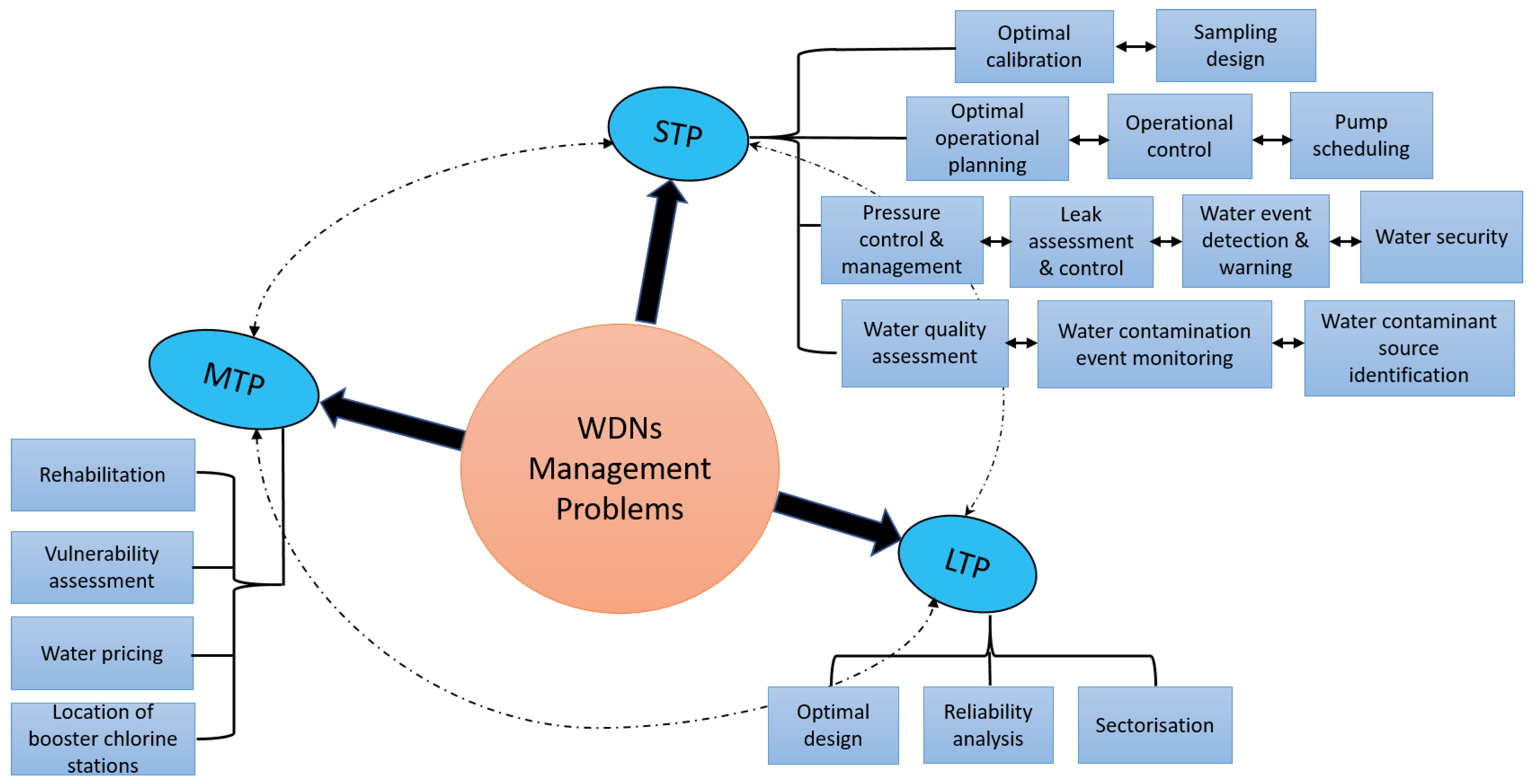
2. WDNs Management Problems and Their Approaches

The management of water distributions networks is essentially meant to meet the varying consumer demand based on the available water supply with respect to the sustainable environmental and financial considerations and reduce drastically the energy costs. The management of water distribution network therefore strives to attain enhanced standards of service delivery to the public and increased customer satisfaction. However, there are events that occur in water distribution networks that affect or degrade the performance of the networks. In the literature, these problems related to the water distribution network are categorized into short-term problem (STP), medium-term problem (MTP) and long-term problem (LTP) as shown in Figure 1, taking into consideration the time horizon on which they usually occur and addressed [2].

2.1. STPs and Approaches

2.1.1. Optimal Calibration

Calibration involves tuning or adjusting a specified set of parameters in the hydraulic simulation and chlorine decay/growth models so that actual behaviour of WDNs can be represented as exact as possible by the models. The adjusted parameters in model calibration are the pipe roughness coefficient, nodal demands, pipe diameter, valve, wall reaction rate constants, and pump operational status. Calibration is achieved by using the measured state variables of the network and the predicted output variables of the model [10].

Earlier efforts to calibrate model were based on iterative (trial and error), model analysis and simulation (explicit) approaches. These approaches are found to have low convergent rate and produce results that are not accurate for intended purposes. The optimization (implicit) approach is the accepted approach to calibrate models due to the possibility of finding optimal decision variables that will reduce the error between the measured and predicted values to the minimum level. The meta-heuristic approaches are preferred to the traditional optimization approaches in that they generate optimal or near-optimal solutions in a broad search space with low computation cost [10,11,12].

The approaches used for calibration of chlorine decay model are manual; and implicit methods. Manual calibration approaches are used to determine the reaction constants using experimental procedures and linear expression. It however has a limited capability to handle many parameters. The implicit calibration method formulates the calibration problem in terms of minimization of objective function subject to constraints that all hydraulic model equations are satisfied, and all specified calibration parameters must be between corresponding search bounds. Implicit approaches are very useful to calibrate models when several parameters need to be adjusted simultaneously. Past studies on calibration of water quality have explored both deterministic and stochastic optimization techniques to solve this problem [10].

2.1.2. Sampling Design

Sampling design is needed to determine appropriate or optimal location for sensors to collect data from WDNs to calibrate a hydraulic and/or water quality model effectively [13]. The simplest methods of sampling design depend on the sensitivity matrix and the covariance matrix of the state parameters by assuming a preliminary estimate of the pipe roughness. These methods involve simulating the network based on the current estimate of the hydraulic parameters and different boundary conditions. Other approaches for sampling design are based on network topology. The network topology-based approaches require initial estimation. It has advantage of producing satisfactory result but do not adequately account for the real number of installed sensors and the need for changing position of previously installed sensors when new sensor is added. A better approach is to formulate sensor location problem as a mixed integer non-linear problem and solve it by optimization techniques.

2.1.3. Optimal Operational Planning

The optimal operational planning of water distribution network is targeted at minimizing the daily operational costs while attempting to satisfy the demand for water by customers at the required quantity, acceptable quality and pressure [14]. Operational cost includes cost of pumping, purchasing, and treating water for a selected operational time horizon. An optimal operating plan is developed to cover at least a period of a day (24 h) divided into wider intervals based on hourly forecast demand pattern and electricity tariffs. Operation planning problem is a difficult and changeling problem to solve due to inherent factors such as the size, topology and types of hydraulic elements of the network [15]. Approaches to solve the optimal operational planning problem include linear programming, dynamic programming, mixed integer programming, evolutionary algorithms, optimization programs linked to hydraulic solver [14]. In addition, software systems that can generate a near-optimal operating plan are available for real-time and online operation of WDNs [16].

2.1.4. Operational Control

Operational control problem in WDNs is concerned with meeting hydraulic performance, economic efficiency, improvement of water quality, storage volume control and other important objectives at minimum cost [3,17]. This is achieved by controlling pumps and valves, keeping the reservoir/tanks levels within specified limits to meet future and unforeseen demands. The optimal control system consists of optimization model that works in conjunction with well calibrated hydraulic and accurate demand forecast models [17].

The approaches to optimal control as highlighted in the literature include hierarchical-decomposition optimization, linear programming, dynamic programming, non-linear programming, integer programming, decomposition-coordination, genetic algorithm, simulated annealing and hybrid optimization methods [3,17]. With the availability of supervisory control and data acquisition (SCADA) systems that provide update information on the current state and the instantaneous operating status of the network, studies are ongoing to develop real-time optimal control WDNs in order to reduce or minimize the operational cost and improve the performance of the network in terms of adequate pressure and flow to meet the demand of the entire networks [3].

2.1.5. Pump Scheduling

Pump scheduling problem is aimed at establishing an optimal policy or set of rules that will enable operators to make decision on the best approach to minimize pumping cost for WDNs while delivering satisfactory level of service to the consumers. The problem is formulated as an optimization problem with the decision variables as the actual pump operating times [18]. Mathematical optimization approaches to solve pump scheduling problem include branch and bound algorithm, Lagrangian decomposition, iterative linear programming, dynamic programming, linearization of system components, and hybrid algorithms. Other approaches to solve the pump scheduling have been dominated by meta-heuristic approaches especially the multi-objective formulations where the final outcome is the optimal Pareto or non-dominated set of operation policies that have optimal trade-off between the objective functions. An excellent review by [19] showed that application of integrated energy and water quality management (EWQMS) would support water utilities to achieve real-time optimal pump scheduling energy efficiency, and water quality objective objectives together with suitable pre-existing SCADA systems.

2.1.6. Leak Assessment and Control

One of the main challenges of the water utility managers is how to minimize water losses to ensure sustainability of finite water resources, protect the environment, improve their generated revenue, and provide high-quality service level to the customers. The coordinated management activities directed to reduce water loss in WDNs include speed and quality of repairs and rehabilitation of failed pipes, pipe materials management, pressure management, active and passive leakage control methodologies [20]. Leakage can be quantified in district metered areas by measuring minimum night flows as used by the authors in [21,22]. The leakage is assumed to be the difference between the minimum night flow and the customers’ night consumption.

There are several approaches to detect and locate leakages in WDNs. Acoustic techniques are the most widely used methods for detecting and locating leakage in water distributions networks. They work by detecting sound waves (acoustic or vibration signals) generated as a result of leakage in pipes. However, the acoustic techniques are labor intensive, expensive, susceptible to external interferences, require significant digital signal processing and not suitable for non-metallic pipes [23].

Apart from the acoustic techniques, other non-acoustic techniques of leak detection techniques for WDNs involve the analysis of quasi-steady-state signals and transient signals (pressure waves) detected by sensors in the pipe network [24]. The use of frequency response functions, cross-correlation analysis, impulse response functions, discrete wavelet transforms techniques, and transient damping techniques were also investigated in the literature to detect leaks in water pipe networks. Leak detection techniques based on transient signals are very complex and may not be practical for underground pipes and field tests [25].

Having identified the need to overcome the computer processing requirements of the acoustic and non-acoustic methods, computational intelligence methods are considered for leaks or burst detection in networks. These computational intelligence tools are trained and validated using a large data set of time series signals and operational data obtained from the field or from hydraulic modelling software to extract leak patterns, classify or predict leaks [26]. Leakage can be identified by correlating changes in flow or pressure characteristics to corresponding changes in the hydraulic model for the network based on the concept of parameter estimation. Significant changes in the hydraulic model show the location and severity of the leakage. A good example is pressure sensitivity method to detect and isolate leaks in WDNs using measured head values and estimated head values from the hydraulic model [27]. Optimization methods based on hydraulic model calibration have been suggested in the literature to locate and reduce leakage in WDNs. The leak detection optimization is usually formulated as non-linear optimization that is solved using traditional and meta-heuristic techniques. The success of this approach depends on the quality of hydraulic model and the available measured data. However, these optimization models have not been widely implemented or verified with real-life networks.

2.1.7. Water Security

WDNs are vulnerable to different sources of intentional or accidental attacks or contamination. The common types of potential attacks are (i) physical, (ii) chemical/biological and (iii) cyber. Malicious or terrorists’ attacks by deliberately introducing chemical, biochemical or radioactive contaminants into WDNs is a major concern for many countries and many guidelines for water quality monitoring and emergency action plants have been proposed [28].

One of the most effective methods to protect water distribution systems is to prevent unauthorized physical access to vulnerable or sensitive locations, lock gates, and provide security surveillance systems. In addition, there should be restriction on access to water distribution maps and network plans. Appropriate computer system security measures should be deployed for the SCADA systems [29].

Another measure to secure WDNs is to provide high level monitoring of pipelines. In addition, water quality monitoring systems are also needed for detection and respond to contamination attacks. Public and government agencies should have plans in advance to deal with emergency responses such as public enlightenment, temporary shutdown of the system, provision of alternative water supplies, cleaning up of the affected area, and emergency health care and treatment to mitigate real or apparent attacks.

Information and communication technologies (ICTs) can play a key role to address various challenges and crisis associated with water management. However, the new ICT techniques required to enhance the water system may itself be a cause of technical problems. For example, the vulnerabilities that inherently reside in wireless communication systems transform into security risks in the water system infrastructures [30]. Therefore, cyber security is a critical component of any ICT-based water management system to ensure the availability, confidentiality, integrity and authenticity of such system and prevent any type of cyber security threats [31].

2.1.8. Water Contamination Event Monitoring

Contamination monitoring systems have been identified as a cost-effective approach to mitigate the risk of accidental or intentional contamination of water distribution networks [32,33]. For effective design and deployment of contamination monitoring systems, the appropriate placement or positioning of sensors within the water distribution network is imperative.

Simple approaches to position sensors to networks involve trial and error method, human experts’ judgement and geographical information system (GIS) data. These approaches may not provide optimal results. Automated method to place sensors is based on application of optimization methods. The sensor placement optimization approach is to achieve overall goal of minimizing the contamination risks. The optimization formulation of the sensor placement problem can be formulated as a single or multi-objective optimization problem with several decision variables, objectives, constraints and assumptions [34]. New studies on the design of wireless sensors, in-line devices and mobile sensors for event monitoring in WDNs are ongoing to enhance water distribution network security [35].

2.1.9. Water Contaminant Source Identification

The source characterization problem entails using observed concentrations at several sensor positions in the network, to detect the contaminant source and its release or temporal mass loading history. The source characterization problem is an inverse water quality problem of simulation a model to monitor usual water quality indicator as pH, Cl, conductivity. This will raise an alarm if some abnormal change is observed. So, the source identification problem uses instead positive and negative responses from sensors. It can be formulated as an optimization problem of finding a source by minimizing the difference between the simulated and observed parameters at the sensor nodes. The approaches to solve the source characterization problem include the use of traditional optimization, meta-heuristics, hybrid and simulation-optimization techniques [36].

2.1.10. Water Event Detection and Warning

Contaminant early warning system is set up to monitor water quality parameters, detect contamination events and provide warning to operators. It should have low false positives and false negatives and to differentiate between normal and abnormal variations in water quality and contaminants events. Event detection subsystem analyses time series data of water quality parameters to provide indication of potential contamination events or abnormal water conditions. The analysis is performed individually for each water quality parameter. The probability estimate for each single parameter is required to produce the event probability through fusing process [37].

The water quality event detection method based on anomaly compares the measured data pattern with the normal data pattern to identify the contamination events using univariate or multivariate statistical analysis. Other anomaly analysis methods for event detection are based on statistical properties, linear predictor, artificial neural networks with Bayesian sequential analysis, support vector machine-evolutionary optimization, minimum volume ellipsoid, data mining or clustering, time-frequency analysis, adaptive updating dynamic thresholds, empirical mode decomposition, binomial event discriminator, Bayesian probability, and optimization techniques [38].

2.1.11. Water Quality Assessment

Water utilities check water quality parameters (microbial and physiochemical) daily or weekly by analyzing samples taken from the WDNs for compliance with guideline values. The analysis of samples, however, is not adequate to detect water quality changes in the networks. With the introduction of online water quality sensors, it is easier and possible to perform online monitoring of water quality parameters. This process monitoring generates large quantities of heterogeneous data that is cumbersome for water utility managers to identify and assess changes in water quality. In addition, the relationship between the water quality parameters and actual water quality is generally non-linear and stochastic in nature. It is very challenging to find approximate mathematical expression to define this relationship. An alternative approach is to use data-based and computationally intelligent techniques to analysis the data and classify water quality [39].

2.1.12. Pressure Control and Management

To reduce pressure to the minimum level and maximize the service level to meet consumer demands, pressure-reducing valves are used for this purpose [40,41,42,43,44,45,46,47]. Alternatively, the pressure can be controlled by maintaining the optimal water levels in the storage tanks as much as the changes in the water demands by customers permit [48]. The challenges of providing pressure management to WDNs are installation, maintenance and replacement costs of pressure-reducing valves and revenue losses due to decrease in water available especially to the pressure dependent customers [49].

An important consideration in pressure management is the determination of location and number of pressure control elements in WDNs. The problem is described as optimal placement of pressure control elements to minimize leakage. Another related problem is to determine the settings of pressure-reducing valves or control valves to minimize leakage while maintaining the security of supply. Composite objective function made up of capital cost of the control elements and cost of leakage is then minimized to solve the optimal placement problem [40,41,50,51].

There are several approaches to solve these problems in the literature as either a single-objective optimization or as a combination of the two or more objectives. These include mathematical optimization-based deterministic optimization techniques to minimize pressure in WDNs and meta-heuristic optimization approaches to control pressure in the WDNs have been investigated. Artificial neural network methods were developed in [1] to achieve real-time optimal pressure-reducing valves setting in water distribution network to reduce water leakage. Other proposed pressure control schemes include predictive and feedback control, proportional algorithm based on the pressure measurements at the control nodes and real-time logic control algorithm [52,53].

2.2. MTPs and Approaches

2.2.1. Rehabilitation

WDNs may deteriorate due to ageing of network elements, leading to pipe breaks, water losses, and inadequate service delivery, compromised quality of water supplied, rising operational, and maintenance costs. It is not feasible to rehabilitate all pipes in an existing water distribution network due to budgetary constraints. Rehabilitation or renewal of WDNs in terms of improving the structural integrity (by replacing physically weak pipes), hydraulic capacity (by cleaning, relining, duplicating or replacing existing pipes); system flexibility or reliability (by providing additional pipe links), water quality (by removing or relining old pipes) of every pipe in the network, requires a methodology that selects rehabilitation option for each pipe in a network and the time of its implementation so as to minimize the rehabilitation and maintenance costs over a specified period of time [54,55]. Recent approaches to rehabilitation problems entail development of decision models based on optimization approaches that take into consideration the cost and performance of the network. The problem is formulated to identify the optimal rehabilitation strategy, within which the selection and timing of the rehabilitation strategy for each pipe is chosen, to minimize the cost of rehabilitation investment and maintenance cost over a predefined time horizon [54].

Studies have been undertaken to apply single- or multi-objective optimization techniques to solve rehabilitation problems in WDNs. The linear, integer, and dynamic programming and meta-heuristic techniques have also been applied to find optimal rehabilitation plans for networks. Recently, decision supports, multi-criteria decision analysis and multi-factor decision making tools were proposed to evaluate and prioritize network rehabilitation alternatives [56].

2.2.2. Vulnerability Assessment

Vulnerability is the analysis of the consequences of failures [57]. Vulnerability of WDNs is caused by physical failure of network elements in particular pipes due to ageing and deterioration. It is important that vulnerable parts in WDNs are identified based on analysis of structural form and connectivity [58,59].

The vulnerability analysis encompasses two steps. Firstly, the building of a hierarchical model of a structure through clustering process in which the members and joints of the structured are agglomerated according to define clustering criteria. Secondly, the hierarchical model is then unzipped until a vulnerable deteriorating event is identified. The hierarchical model is unzipped from the top to bottom focusing on all the existing network branch clusters. Physical vulnerability index can be used to measure the consequences of failure in a network. Its value varies between zero and one where the higher values indicate higher level of vulnerability. In case of intrusion of contaminants in water distribution systems, the indices to evaluate the characteristics of the nodes are the hazard index and vulnerability index. The hazard index of a node is obtained by assessing the comprehensive impacts of contaminant events in the water distribution network when the pollutant was injected at a particular node. The vulnerability index of a node is computed by assessing the comprehensive impacts of contaminant events on a particular node when the pollutant was injected from the other nodes [57].

2.2.3. Water Pricing

Water pricing is an instrument used by water utilities for the purpose of financial sustainability through cost recovery. In determining the price of water, the forces of supply and demand are important considerations. The water suppliers and buyers are one of the key agents in the water industry [60]. Constant unit pricing scheme is simplest form of water pricing. It supports financial sustainability but may deprive low income earners and poor access to potable water. Marginal cost pricing (MCP) is another scheme where the water supplier makes effort to maximize social welfare. The limitations of MCP are the lack of budget constraints, absence of information of fixed costs and inclusion of administrative cost.

An alternative to the MCP is the two-part tariff that includes the fixed charge that covers capital asset renewal and debt servicing, and the marginal cost price that corresponds to the operating expenses. To account for budget constraints, an improved model of average cost pricing called “Ramsey-Boiteux” pricing was developed. It ensures the maximal economic welfare under budget constraint is realized. Block rate pricing scheme is also a solution to the problem of excess profits and losses associated with the MCP. The block rate has ability to charge the poor customers lesser than the richer and bigger customers, to promote economic efficient, and to penalize customers that waste water. One of the limitations of the block rate pricing is that it gives openings for customers to move from an expensive block to less expensive block, thus affecting the revenue of the water utilities. Optimal non-linear pricing based on multi-block price system with social considerations was proposed in [61] to solve water pricing problem.

2.2.4. Location of Booster Chlorine Stations

Re-chlorination is considered to be one of the essential approaches to maintain adequate chlorine residuals that decrease due to long residence times in buffers. The simplest approach to address the problem of reduction in free residual chlorine concentration is to increase dosages at the water source. However, this approach may lead to higher free residual chlorine concentration for customers near these water sources and support formation of disinfection by products that are harmful to public health [62]. A more realistic approach is to introduce booster chlorine station or injectors to supply the sufficient quantity of chlorine require at critical locations throughout the network. Thus, the main issue about re-chlorination is the optimal placement of booster chlorination stations and setting of the required chlorination dose of the boosters. It is challenging due to lack of adequate knowledge about the variations of free chlorine residuals along networks.

One of the methods to solve the problem is using chlorine contour maps. The water utility managers can use it to decide the need to add booster stations to networks and find the accurate locations for the stations [63]. The most widely approach is to use optimization-simulation techniques to solve the design and operation problem of booster chlorine stations that is formulated as a non-linear programming problem [62].

2.3. LTPs and Approaches

2.3.1. Optimal Design

In a simplified approach, the problem of optimum design of WDNs is to determine the combination of L number of pipes and D commercially available discrete pipe diameters to construct a new network or modify an existing network at a minimum total cost without violating the hydraulic constraints. The least cost problem design is formulated as a non-linear mixed integer problem. The simplified objective function can be elaborated by considering additional cost associated with the valves, pumps, reservoirs, tanks and other special hydraulic appurtenances that are components of the network [64]. Furthermore, with ever-increasing population and urbanization, the demand for water is growing at an alarming rate. These scenarios which prompt the need for demand development (connections to community level plans) are important part of the long-term level water management problems. There are several approaches that have been proposed [65,66,67,68] but the meta-heuristics techniques are most preferred methods due to their ability to find close-to-optimal solutions to the problem within reasonable computing times [69].

The multi-objective optimization of water distribution network design is a new direction that is drawing attention of researchers presently. The approaches in multi-objective optimal design is to find a set of different solutions that together show the best possible multi-objective trade-off surface, known as the Pareto optimal front. In the simplified least cost design of water distribution network, it is assumed that all hydraulic model input variables are accurately known. However, in practical networks, quantities such as nodal demand and pipe roughness coefficients are uncertain and are therefore considered in some studies to avoid under-design of networks. This is referred to as stochastic or robust optimal design problem. The robustness effect of the uncertain model inputs is thus quantified and evaluated on the model output variables using either sampling-based or analytical-based techniques [70,71]. A framework for a real-time dynamic hydraulic model as an effective approach to implementing an efficient, reliable and adaptive networks that can replace the current steady-state hydraulic models which have inherent limitations with respect to reliability and efficiency was proposed in [72]. In the proposed system, several network parameters need to be sensed and directly fed into the model. The dynamic model will use the real-time sensed data to evaluate the current conditions of the network and automatically send control signals to various network components.

2.3.2. Reliability Analysis

Reliability is generally defined as the probability that a system performs its task within a specified period of time and under specified conditions. Reliability is a probabilistic event and it may predict where and when pipe, valve and pump will fail [73]. Reliability analysis of WDNs can be separated into mechanical, topological, and hydraulic reliability studies. Mechanical reliability relates to the probability that mechanical components of a network will not fail or remain in operation [74,75].

There are analytical methods such as path enumeration, state enumeration, and simulation methods such as Monte Carlo Simulation that are discussed in the literature to calculate the reliability of networks based on estimated values of the probability of operation or failure of each link. The analytical methods can provide a fast initial assessment of the reliability of a network. However, stochastic simulation method enables computation of a much broader class of reliability measures than do analytical methods, but it requires significant amount of computer time and less easy to generalize [74,75]. Reliability analysis is performed by simulating several scenarios representing all the expected states of the network. The results of the simulations are successfully displayed in terms of any of the following indices: nodal reliability indicators for water demand, pressure, water quality, modified resilience index, entropy function, minimum surplus head index, and resilience index [76,77]. It should be emphasized here that reliability of WDNs is difficult to define and calculate. In fact, there are no universal definitions for reliability indices or indicators.

2.3.3. Sectorization

The process of partitioning a water distribution network into a set of independent district metered areas is called sectorization. It used to achieve better control over the network, enhance leakage and burst detection and management, pressure management, control of contamination spread, enhance water security, improve work planning and rehabilitation, and support effective monitoring and control of the activities and operation of the network. Partitioning of WDNs reduces the redundancy of the layout of the network significantly and loss in the system resilience if the design is poorly done [78,79].

The district metered areas are formed by placing and closing boundary or isolation valves along certain pipes connecting one district metered area to another (closed links) and placing a flow meter in the remaining connecting pipes (called open links) in WDNs [80]. Thereby, discrete areas are created and flow into each discrete area is monitored [81,82]. The traditional approaches to the design of district metered areas are based on trial and error method and empirical techniques with emphasis on the number of properties or consumers, length of pipes using hydraulic simulations. Other improved techniques for re-designing existing WDNs into independent areas include graph theory algorithms such as breath first search and depth first search, and optimization techniques [42,83].

Most of these water management problems are linked with one another. For instance, the rehabilitation analysis is strongly linked with the leakage assessment and control, the pressure control and management, as well as the steady-state models. Leakage assessment as well as the pressure control management may be used to predict the behavior and failure of the system to event such as pipe burst, high pressures, and pressure-deficient conditions. Also, some hydraulic models (pressure-driven analysis) has been used to assess the response of the water system in case of low or negative pressures. The sectorization is linked, among others, with the pressure control and management, operational control, and the sampling design. A particular section of the water supply network such as the discrete meter area (DMA) could be partitioned where the pressure at the inlet of such area control for leakage reduction and pressure management. Also, some flow or pressure sensors may be positioned at the DMAs for real-time measurement of pressures and flow rates. It is important to state that in problematic situations such as quality problems, there might be sampling design also on the short-term level for measurement campaigns.

3. Mathematical Models Used in WDNs Problem Solving

In WDNs, mathematical models are used to describe and emulate the behavior or responses of networks, and estimate the states and parameters of the networks for some specific operating and loading conditions. In this section, some of the salient mathematical models adopted to assist in solving management problem in water supply system is discussed.

3.1. Steady-State and Dynamic Hydraulic Models

The steady-state hydraulic model calculates the network hydraulic variables at a particular instant of time. It gives the snapshot of the WDNs. The first Kirchhoff conservation law (mass conservation) is used to describe the flow conservation at the nodes in a pipe network:

$$\sum _i{q}_{i,j}=Q_{j}j=1,\dots ,J,\left(\mathit{Junction}\mathit{nodes}\right)$$

(1)

where $q_{i,j}$ is the flow in link connecting nodes i and j, J is the number of nodes, $Q_j$ is the demand at the node, j.

The second Kirchhoff law of conservation law is also known as law of conservation of energy. It states that the total head loss around any network loop is zero.

$$\sum _{i,j\in m}{h}_{i,j}=0m=1,\dots ,M,\left(\mathit{Loops}\right)$$

(2)

where $h_m$ is the head loss of the pipe $(i,j)$, and M is the number of loops. For the sake of simplicity, we assume here there is only one tank so that there is no need for pseudo-loops between fixed head nodes. This will be generalized later.

The third equation required to model the network, shows the relationship between the flow and head loss. This relationship is in form of Ohm’s law. The expression in a simplified form is represented as:

$$h_{i,j}=R_{i,j}\mid q_{i,j}{\mid }^{n-1}{q}_{i,j}$$

(3)

where $R_{i,j}$ is the resistance of the pipe connecting nodes i and j and n is a fixed head loss exponent. This is also applicable to valves with a resistance coefficient that depends on some local head loss coefficient and the valve diameter.

A pump generally has a characteristic curve which describes the relationship between the head gain and flow. This can be approximated by a parabolic function:

$$h_{i,j}=a_k{q}_{i,j}^2+b_k{q}_{i,j}+c_k$$

(4)

where $a_k$, $b_k$ and $c_k$ are the coefficients of characteristics provided by the pump manufacturers. Equation (4) is only valid in a specific range and this (the domain and the definition of the function) must be extended to get a monotonic function for the head loss, which guarantees the existence of a solution [84].

The combination of (1)–(4) forms a set of non-linear equations describing the steady-state behaviour of WDNs. The flows and heads in the WDNs are the solutions of these equations when all the pipe resistances, characteristic curves (pipe and pump parameters), node demands, reservoir levels, number and speed of working pumps, and degree of valve opening (operating conditions) are known.

A direct mathematical solution to solve this large system of non-linear equations simultaneously is not feasible. However, some analytical and numerical techniques have been proposed to solve these steady-state equations. The first method to be proposed for solving the equations is the Hardy-Cross method. This method is based on the Newton method applied to the loop or node equations. However, in the Hardy-Cross method each of the equations is taken sequentially (a relaxation method), which comes back to ignore the non-diagonal elements of the Jacobian matrix. This leads to very slow convergence and makes the solution of large problems infeasible.

On the other hand, solving the nodal equations, with the pressures as variables, leads to equations with square roots and reduced convergence compared to the loop systems using the corresponding Newton-Raphson method. The first method to be proposed capable of solving large network problem was the hybrid method by Hamam and Brameller [85]. This method possesses the convergence of the loop method and the solution of the linearized equations, at each iteration, using the nodal representation with its intrinsic sparse properties. Since the hybrid method was proposed, other methods have been suggested. These include: variational formulation [86], global gradient method [87]; Perturbation or delta expansion [88]; Newton-Raphson, linear methods [89]; extended linear graph theory [90,91]; Node-loop method [92]; Gröber basis [93]; and improved variational formulation method [94].

The dynamic hydraulic model or extended-period simulation (EPS) describes the hydraulic behavior of WDNs with changes in time [72]. This is generally formulated to include the law of conservation of mass for a node with tanks or storage elements and is given as:

$$\sum _i{q}_{i,j}-Q_j-\frac{d{V}_j}{dt}=0$$

(5)

where $V_j$ is volume of the tank at the node j and t is the time. Assuming the head (sum of tank level and elevation) and cross-sectional area of the tank are represented by $H_j$ and $A_j$ respectively. The dynamic expression of the tank can be written as:

$$A_j\frac{d{H}_j}{dt}=Q_j^I=\sum _i{q}_{i,j}-Q_j$$

(6)

Extending the (6) for a network that has several tanks. The dynamic model of the network can be expressed by a set of differential equations:

$$\mathbf{A}\frac{d\mathbf{H}}{dt}={\mathbf{Q}}^I$$

(7)

where $\mathbf{A}$ is the vector of the cross-sectional areas, $\mathbf{H}$ is the vector of tank heads, and ${\mathbf{Q}}^I$ is the vector of net tank inflows.

The tank differential Equation (7), may be suitably solved using numerical methods such as numerical integration (forward Euler, improved Euler), hybrid transient and explicit integration methods. A comprehensive description of these methods can be found in [89].

Generally, it is assumed that water demands by the users are lumped together at the nodes where the pressure heads are determined. However, in reality, water demands are distributed irregularly along the pipes. Thus, approximating and allocating user demands to the nodes may give unsatisfactory calibration results and pipe head loss errors. Some methods have been proposed to address this limitation in hydraulic model analysis [91,95]. However, this is an important area that future research could be directed to propose novel techniques to analyze models of water distribution networks that account for both uniformly and unevenly distributed users demand along pipes in WDNs.

3.2. Connected Graph Models

A water distribution network can be described by connected graphs comprising a finite number of interconnected elements. A graph element consists of an oriented edge and its two distinct endpoints or vertexes. Each edge has a defined length, diameter, and roughness. Edges may represent pumps, valves, meters, bends, pipes and any other hydraulic elements that have a known head loss/flow relationship. The endpoints are known as points of intersection (junction nodes) or points of connection to tanks or water sources (datum nodes). The general mathematical expression for a connected graph containing edges, e, junction nodes, n, and datum nodes, s, can be formulated using governing principles of mass and energy conservation [96,97]. The law of continuity can be stated as:

$$\sum _{i=1}^e{\lambda }_{j,i}{q}_i+Q_j=0;{\lambda }_{j,i}\in \{-1,0,1\}\mathrm{and}j=1,\dots ,n$$

(8)

or in a more compact form

$$[\Lambda ]\left\{q\right\}+\left\{Q\right\}=\left\{0\right\}$$

(9)

This shows that at each junction node, the sum of inflows $({\lambda }_{j,i}=-1)$ or outflows $({\lambda }_{i,j}=1)$ must be zero. $\Lambda$ is the incidence matrix reduced to junction nodes, q is the edge flow rate and Q is the external junction demand.

The law of energy balance or conservation indicates that the algebraic sum of head loss h must equal zero for a closed loop, or the difference of the end-point heads for non-closed-loop. It is denoted as:

$$\sum _{i=1}^e{\gamma }_{m,i}{h}_i+{\varphi }_m=0;{\gamma }_{m,i}\in \{-1,0,1\}\mathrm{and}m=1,\dots ,M+s-1$$

(10)

or in more compact form

$$[\Gamma ]\left\{h\right\}+\left\{\varphi \right\}=\left\{0\right\}$$

(11)

where the $\varphi$ components are zero for fundamental circuits. $\Gamma$ is the loop matrix.

As discussed above, edges may represent various hydraulic elements that have a known head loss/flow relationship. The head loss variable, h, is a non-linear characteristic function of the flow rate and stated as:

$$h={R\left|q\right|}^{n-1}q\mathrm{or}a{q}^2+bq+c$$

(12)

where the first term in Equation (3) refers to a pipe or valve, and the second term in Equation (4) to a pump.

3.3. Detailed and Reduced Hydraulic Models

Real WDNs usually contain thousands of nodes and links that are highly interconnected. The spatial data of these networks could be generated from the GIS of cities or towns with more detailed information. These detailed models are useful to determine the hydraulic states at any point on the networks. Some commercial and free software packages exist that could easily assist to perform modelling and analysis of WDNs using the information from the GIS database. Detailed models are required to solve some management problems associated with the networks. These include leakage detection and control [24], water quality analysis, network enhancement, or upgrade. It should be pointed out here that it is difficult to calibrate a detailed model because all the current state measurements of the network may not be available at the time of calibration [98].

However, there are problems in the networks that require reduced models to solve them. In these instances, the detailed models could be reduced or skeletonized into a single “equivalent pipe” for each of the considered applications and tuned as close as possible to the real-life network. The key goal of the reduced models is to faithfully represent the non-linearity of the detailed models and approximate its behavior under different scenarios. Optimal network design, operation, and pump scheduling problems are solved using reduced models. Availability of key operational conditions and parameters, with associated costs and constraints to be met, are necessary to solve these problems using reduced models [10].

3.4. Offline and Online Hydraulic Models

Offline mathematical models are network representations that have parameters that are not continuously updated to show the current states of the network. Most of the hydraulic modelling software packages are based on offline models. To apply these models, offline models are calibrated based on a substantial amount of historical data once in a specified period of time. However, these calibrated offline models are inadequate to meet real-time operational needs of networks and cannot access current network information to drive simulations.

The online models are developed from calibrated offline models that are linked to supervisory control and data acquisition systems that provide current, near real-time measurements of flow and pressure in the WDNs. The online model parameters are updated based on current measurements. For instance, at every 15 min, the online model automatically performs continuous cycle of simulation runs and model outputs are stored in the database [99].

3.5. Microscopic and Macroscopic Hydraulic Models

Microscopic models are developed from first principles governing WDNs as described in Equations (1)–(7). They are full or reference simulation models with exact link parameters (diameter, length, roughness), nodes, topologies of the networks are known, and nodal demands must be estimated in advance before they are applied to solve problems on WDNs.

On the other hand, macroscopic models are based on empirical modelling techniques. They are developed and updated by operational data especially major flows and heads related to tanks and pumps in the networks. Macroscopic models are suitable for solving optimal control and operation problems in WDNs. These models can be in form of regression models, artificial neural networks and other data-based models [100,101,102]. Although these models are very different in detail, a macroscopic model of a water distribution network in discrete-time can conceptually be represented as:

$$x(k+1)=f\left(\left(x\right(k),u(k),d(k),\epsilon (k)\right)$$

(13)

where $x\left(k\right)$ is the vector of state variables. The state variables include nodal pressure, pipe flow, and tank depth. The state variables at time $k+1$ are determined from the state variables at time k and the following additional quantities. $u\left(k\right)$ is a vector of control variables. The control variables include outlet pressure and flow of pumping stations, and the discharge through the flow control valves. $d\left(k\right)$ is a vector of the nodal demand distributed in the network. $\epsilon \left(k\right)$ represents the stochastic disturbance and f is a non-linear function of the network.

3.6. Demand-Driven and Pressure-Driven Analysis Models

Demand-driven analysis models are based on the assumption that nodal demands are fully known and are not dependent on the pressure at the nodes. This simplified assumption is used in most of the hydraulic models for WDNs. However, this may lead to incorrect or negative nodal pressure in the analysis and simulation of the hydraulic models that fail to indicate the actual state of the network [103].

In practical situations, the demand at each node actually depends on the nodal head. The nodal demand is not constant. This means that as the nodal head changes, the actual demand by the consumers is affected. Therefore, another model known as the pressure-driven analysis model was developed and applied to account for this effect. To replace the nodal demand in the general hydraulic equations, a relationship between nodal head and nodal demand is given as [104]:

$$\begin{array}{c}\hfill \left\{\begin{array}{cc}{Q}_j^{av}=Q_j^{rq},\hfill & \hfill H_j>H_{rq}^j\\ Q_j^{av}=Q_j^{rq}{\left(\frac{H_j-H_j^{min}}{H_j^{rq}-H_j^{min}}\right)}^{\left(\frac{1}{n}\right)},\hfill & \hfill H_j^{min}\le H_j\le H_{rq}^j\\ Q_j^{av}=0,\hfill & \hfill H_j\le H_{min}^j\end{array}\right.\end{array}$$

(14)

where $Q_j^{rq}$ is the required demand at the node j, $Q_j^{av}$ is the available demand at node j, $H_j$ is the available head at node j, $H_j^{rq}$ is the minimum required head or design head, $H_j^{min}$ is the minimum head and n is the head exponent that is between 0.5 and 2. In practice, Equation (14) means that there is no demand at the node if the head at the node is less than $H_j^{min}$, and that the required demand is fully met for head more than $H_j^{rq}$. For a head between $H_j^{min}$ and $H_j^{rq}$ the demand is interpolated between zero and the required demand.

In the literature, Equation (14) is regarded as the basic expression to determine head dependent demand at each node of a network. A review of other explicit relationships between the nodal head and outflow can be found in [105]. However, these head-demand relationships have limitations such as convergence difficulties due to discontinuity in their derivatives at the transitions between zero and available nodal demand and/or between available and required nodal demands, among others. The need to solve the head-demand relationship with better computational properties for networks with passive elements was addressed in [106]. The study proposed robust and rapidly convergent methods to solve the head-outflow relationship using co-content and weighted least square optimization models with Goldstein’s line search algorithm. However, other novel methods to solve the head-outflow relationship for networks with active elements and extreme operational conditions are desirable.

3.7. Hydraulic Transient Models

The transient flow in WDNs can be described by the following expressions known as water-hammer equations [107]:

$$gA\frac{\partial H}{\partial x}+\frac{\partial q}{\partial t}+\frac{f}{2DA}q\left|q\right|=0$$

(15)

$$\frac{\partial H}{\partial t}+\frac{a^2}{gA}\frac{\partial q}{\partial x}=0$$

(16)

where H is the hydraulic head, x is distance, t is time, f is the friction factor, D is the pipe diameter, A is the pipe cross-sectional area, q is the flow in the pipe, a is wave speed, and g is the gravity acceleration.

By applying the method of characteristics, Equations (15) and (16) can be transformed into the following sets of ordinary differential equations along the characteristic lines $({\displaystyle \frac{dx}{dt}}=\pm a)$

$$\begin{array}{c}\hfill C^{+}:\left\{\begin{array}{c}\frac{dH}{dt}+\frac{a}{gA}\frac{dq}{dt}+\frac{fa}{2gD{A}^2}q\left|q\right|=0\hfill \\ \frac{dx}{dt}=+a\hfill \end{array}\right.\end{array}$$

(17)

$$\begin{array}{c}\hfill C^{-}:\left\{\begin{array}{c}-\frac{dH}{dt}+\frac{a}{gA}\frac{dq}{dt}+\frac{fa}{2gD{A}^2}q\left|q\right|=0\hfill \\ \frac{dx}{dt}=-a\hfill \end{array}\right.\end{array}$$

(18)

where $dx$ is the distance differential and $dt$ is the time differential.

The approximate solutions of Equations (17) and (18) give the transient heads and flows at the grid points in the network simultaneously. The solutions can be obtained using the finite difference method with the selection of suitable initial and boundary conditions (based on known heads and flows in the network). The frictional factor f of each pipeline can be determined through Darcy-Weisbach equation with parameters being pipe length L, pipe diameter D, head loss h and flow velocity v obtained from the steady-state network simulations as:

$$h_{ij}=f_{ij}\frac{L_{ij}{v}_{ij}\left|v_{ij}\right|}{D_{ij}2g}$$

(19)

3.8. Water Quality Models

Water quality models are found applicable for tracer studies in WDNs (travel times and flow paths), determination of sampling locations, analysis of contaminants/disinfectant concentrations, water age simulation, water quality operation optimization, source contaminant detection and location, location and operational optimization of disinfectant booster stations, and water quality sensor location design [10,108,109]. Water quality models are used together with hydraulic models to solve water quality issues in WDNs. These models are important tools to predict water quality transport and fate in WDNs [110].

The propagation of contaminants or substance in WDNs is made up of the following processes: advection in pipes; kinetic reaction mechanism; and mixing at nodes. The steadily flowing contaminants in a pipe can be expressed by a one-dimensional mass conservation differential equation of the form [97,111]:

$$\frac{\partial C}{\partial t}=-\frac{q}{A}\frac{\partial C}{\partial x}+\theta \left(C\right)$$

(20)

where C is the contaminant concentration within the pipe, q is the pipe volumetric flow rate, A is the pipe cross-section area, x is the distance along the pipe in the positive flow direction, $\theta \left(C\right)$ is the rate of reaction of contaminants within the pipe.

The changes in the contaminant concentration in the pipe can be expressed by a first-order kinetic rate equation:

$$\theta \left(c\right)=kC$$

(21)

where k is the first-order reaction rate coefficient and C is the contaminant concentration in bulk flow. For processes that involve contaminant growth, the coefficient is positive while for processes that lead to decay of contaminants, the coefficient is negative.

The mixing at the node can be obtained from the mass balance principle stated as follows:

$$C_k=\frac{{\sum }_{j\in \left\{k\right\}}{q}_j{C}_j}{{\sum }_{j\in \left\{k\right\}}{q}_j}$$

(22)

where $C_k$ denotes the contaminant concentration at node k, k is the set of incoming pipes.

For pumps and valves that are active elements, it is assumed that the incoming and outgoing contaminant concentrations for these elements are the same (instantaneous contaminant advection). For a variable-level tank, the change in concentration of contaminant can be expressed as:

$$\frac{d\left(C_T{V}_T\right)}{dt}=q_{in}{C}_{in}-q_{out}{C}_T+{\theta }^{\prime }\left(C_T\right)$$

(23)

where $C_T$ and $V_T$ are the fully mixed concentration and volume of the tank, respectively, $C_{in}$ is the contaminant concentration of the incoming pipe, and ${\theta }^{\prime }\left(C^T\right)$ is the reaction rate within the tank.

The assumed complete mixing at the nodes and tanks are meant to simplify the analysis of the water quality model. There are other forms of mixing models that have been studied with the aid of computational fluid dynamics that could be helpful to develop more accurate water quality models [33,98,112].

3.9. Demand Forecast Models

Accurate prediction of peak water demands stems from the need to improve or optimize the operation and management of WDNs. Water demand forecasting is an important tool for the design, operation, and management of WDNs. It is based upon the past water use, and socio-economic and climate parameters associated with the past water use. These parameters are precipitation (rain), temperature, seasonality, and evapotranspiration, water price, income, family size and other related factors [113,114,115,116]. Short-term water demand forecasting is essential for operation and management of networks whereas long-term forecasting is required by utility managers for planning and design of WDNs. In the literature, several modelling techniques for water forecasting are discussed which can be classified as conventional, machine learning, or a combination of both conventional and machine learning techniques.

Conventional modelling techniques include regression-disaggregation and time series analyses. Regression-disaggregation starts with the development of a weekly demand forecast regression model and later change into daily values through a disaggregation process. The current water demand is thus predicted using the following expression [117]:

$$D_W\left(t\right)=\alpha D_W(t-1)+\beta P\left(t\right)+\gamma P(t-1)+\delta T\left(t\right)$$

(24)

where $D_W\left(t\right)$ is the demand in week t (million liters per day), $D_W(t-1)$ is the demand in week $t-1$ (million liters per day), $P\left(t\right)$ is the rainfall in week t (millimeters), $P(t-1)$ is the rainfall in week $t-1$ (millimeters), $T\left(t\right)$ is the temperature in week t (degrees Fahrenheit); and $\alpha$, $\beta$, $\gamma$ and $\delta$ are regression parameters of $D_W(t-1)$, $P\left(t\right)$, $P(t-1)$ and $T\left(t\right)$ respectively to be estimated.

The forecast weekly demands are then disaggregated into daily water demands using moving average disaggregation model (MADM) or mean seasonal average disaggregation model (MSADM).

Time series models for water demand on a day t can be formulated as [117]:

$$D\left(t\right)=B\left(t\right)+L\left(t\right)+S\left(t\right)+A\left(t\right)+R\left(t\right)$$

(25)

where $D\left(t\right)$ is the daily demand on day t (million liters per day), $B\left(t\right)$ is the basic water demand component that is the minimum water demand for the city obtained from the historical records, $L\left(t\right)$ is the long-term demand component that represents the any long-term trends in the annual average water demand over the years, $S\left(t\right)$ is the seasonal demand component that accounts for the seasonal variations in the daily water demand over a year, $A\left(t\right)$ is the autocorrelation component shows the dependence of the current water demand on the past water demand, and $R\left(t\right)$ is the random component accounts for any uncorrelated uncertainties associated with the water demand time series.

Assuming, the long-term demand component $\left(L\right(t)=0)$, further manipulation of Equation (25) can be stated as:

$$D\left(t\right)=g\left(t\right)+I\left(t\right)$$

(26)

where $g\left(t\right)$ is the combined seasonal and basic water demand component and $I\left(t\right)$ is the combined autocorrelation and random component.

Alternatively, Gato et al. [118] suggested that the water demand forecast can be obtained as the sum of the estimated daily base demand and daily seasonal demand of water. This can be expressed as:

$$W_d=W_b+W_s^p+W_s^c+W_s^r\left(d\right)$$

(27)

where $W_b$ is the base demand (million liters per day), $W_s^p$ is the potential seasonal demand, $W_s^c$ is the weather component of seasonal demand (million liters per day) and $W_s^r\left(d\right)$ is the persistence component of seasonal demand (million liters per day).

In view of the large number of interacting variables associated with water demand forecast, the representation of this complex process with conventional statistical techniques often lead to inaccurate prediction. Computational intelligence techniques are now being employed to forecast water demands due to their ability to model non-linear processes accurately without using complex mathematical expressions. With the availability of input-output datasets, the models are trained, tested, and validated by historical datasets. Examples of these techniques are rule-based expert systems, artificial neural networks, dynamic artificial neural networks, combined expert network model, projection pursuit regression (PPR), multivariate adaptive regression splines (MARS), support vector regression (SVR), and random forests, support vector machines (SVM), fuzzy logic, adaptive neuro-fuzzy inference system, Bayesian maximum entropy, agent-based models, system dynamic models and hybrid methods [113,117,119].

3.10. Water Leakage Models

A general expression called the Torricelli equation is used to relate pressure head and leakage in a pipe, where the leak is assumed to be an orifice [120,121,122,123,124,125]. This is stated as:

$$Q_L=C_{d}A\sqrt{2gH}$$

(28)

where $C_d$ is the discharge coefficient, A is the area of the orifice, H is the pressure head in the system and g is acceleration due to gravity. The exponent of the pressure head is by default 0.5.

However, studies have shown that the leak behaviour is more complex than assuming that it is an orifice. The pressure exponent in practice is in the range of 0.5 to 2.98. A power equation is thus derived as an expression of water loss in practice, to describe the relationship between pressure head and leakage:

$$Q_L=c{H}^{N_l}$$

(29)

where $Q_L$ is the leakage flow rate, c is the leakage coefficient and $N_l$ is the leakage exponent.

Another proposed model to describe the leakage behaviour is based on the fixed and variable area discharge (FAVAD) leakage concept. This approach assumes that some leaks are fixed $(N_l=0.5)$ while other leaks are varying with increasing pressure. The combined leakage equation, which is a modified form of the power equation, is

$$Q_L=c_1{H}^{0.5}+c_2{H}^{1.5}$$

(30)

where $c_1$ and $c_2$ are the coefficients characterizing the fixed leaks and variable area leaks, respectively. From experimental studies, the area of any leak undergoing elastic deformation can be denoted as [120]:

$$A=A_0+mH$$

(31)

where $A_0$ is initial leak area and m is the head-area slope.

Then, substituting Equation (31) into Equation (28) gives

$$Q_L=C_d\sqrt{2g}\left(A_0{H}^{0.5}+m{H}^{1.5}\right)$$

(32)

Comparing Equation (30) and Equation (32), the leak coefficients can be defined as $c_1=C_d{A}_o\sqrt{2g}$ and $c_2=C_{d}m\sqrt{2g}$.

The FAVAD model is thus useful to describe the behaviour of many leaks in WDNs. To simulate and analyze the FAVAD leakage model incorporated into a steady-state hydraulic model, a study was performed by Piller and van Zyl [126], where a damped Newton method was proposed as a viable approach to solve the problem.

Adedeji et al. [127] presents an overview of the pressure management approaches proposed for reducing leakages in WDNs, such as fixed outlet pressure control, the time-modulated pressure control and the flow modulated pressure control strategies. Page et al. [128] investigates the robustness of parameter-less remote real-time pressure control in water distribution systems. Parameter-less control can be used to manage the pressure to be as low as possible, which will reduce water leakage, pipe bursts, and water consumption in a water distribution system. Parameter-less remote real-time pressure control is based on the flow and can be used to control a pressure control valves [129,130] as well as variable speed pumps [131,132].

3.11. Optimization Models

One of the versatile models for solving management problems in WDNs is the optimization model. The essence of optimization is to minimize the total cost involved in solving a particular problem, reduce errors between the measured and simulated values or maximize performance indices. Optimization techniques search for the best solution from all possible solutions. The objective functions of the water distribution network problems are usually conditioned by physical mass and conservation laws, head loss/flow relationships, minimum pressure requirements at the demand nodes and other important inequality or/and equality constraints depending on the problem under consideration. The decision variables can be in form of continuous or discrete values that indicate a set of solutions to the optimization problems [7].

There are several approaches that have been proposed and extensively discussed to solve optimization problems relating to WDNs. These approaches include enumeration, linear programming, non-linear programming, dynamic programming, integer programming, stochastic or meta-heuristics, and hybrid optimization (fusion between traditional and meta-heuristics) techniques. The different approaches are reviewed in [7,133]. Of all these approaches, the meta-heuristics technique is the preferred method due to its ability to find close-to-optimal solutions to problems within reasonable computing time [7,133,134].

A single-objective optimal problem can be described as:

$$\mathit{Min}f\left(x\right)$$

(33)

subject to Equations (1)–(3) and any other relevant constraints. Here $f\left(x\right)$ is the objective or cost function of the network to be minimized.

In recent times, most management problems in WDNs were formulated as multi-objective optimization. It has more than one objective function to be optimized. The approaches to multi-objective optimal problems may involve getting a set of different solutions that together give the best possible multi-objective trade-off surface, known as the Pareto optimal front. Although there are several alternatives to solve multi-objective optimization problems, it is preferable to use approaches that will find the Pareto optimal front with very few iterations before a final solution is selected from a set of non-dominated solutions [99,135,136].

Most of these models have been used as a tool in solving water management problems which are short-term, medium-term, and long-term, to improve operation, capability, and performance of WDNs, and to ensure uninterrupted service to customers. For instance, hydraulic behavior of the networks is described using the steady-state and dynamic hydraulic models, water quality models are useful to explain the contaminants transport processes, while minimization models are used to optimize system errors or cost of operation, network rehabilitation, and design, among others. The steady-state hydraulic mode (the demand-driven and pressure-driven) have been used to appraise leakage behavior and pressure management and control in the water networks. They have been used for operational planning and optimal design in the estimation of pipe diameter size and roughness needed for the design of water piping networks. Also, water leakage models are being used for leakage assessment and control as well as pressure control and management. These mathematical models in the form of computer algorithms could be developed based on various modelling approaches to provide fast solutions subject to the fundamental laws of mass and energy conservation, governing WDNs [137,138,139]. Demand forecasting models have been used for water pricing and the operational control based on the social economic impact of water savings and demand.

4. Future Directions

The list of study areas in the future is presented in this section. These lists entail the future research studies in the WDNs management problem approaches and the mathematical models used.

Calibration and sampling design: There is a need to have pressure-driven analysis-based model that can perform simultaneous calibration of the demand pattern, pipe diameters, pipe roughness coefficients and valve/pump status of WDNs. An improved framework for continuous calibration of hydraulic and water quality models through regular updating is required.

Operational control: Novel, high performance and robust control algorithms should be proposed to regulate water volume in each tank and/or water level in reservoirs to ensure availability of adequate drinking water for daily consumption (water storage control) and flow through the network to meet future demand at required pressure head levels (flow control).

Pumping scheduling: New algorithms to solve simultaneous optimization of pump and valves schedules to minimize energy and maintenance costs should be proposed. Real-time implementation of pump scheduling with fast computation time on real WDNs should be investigated.

Operation planning: New and advanced optimization methods to solve operational planning problem in medium and large network with least computational resources should be further studied. Versatile and easy to use decision support systems should be developed for operational planning of WDNs.

Leakage management: There should be further investigations into the development of low cost automatic early burst detection system for service pipes and water mains by devising intelligent algorithms. Efficient and effective decision support systems for water utility managers to perform online leakage detection/localization, evaluate, and rank potential actions for leakage control and management should be proposed.

Pressure management: It is important that future studies relating to application of more efficient optimization methods to find the number and location of pressure-reducing valves, and adjustment of valves opening adjustment to control pressure in the network simultaneously should be examined. Implementation of real-time control of valves to achieve leakage reduction in real WDNs should be carried out.

Water security: More efficient optimal response protocols and dynamic decision support models that will assist water utility managers and staff to take the best emergency response actions during water contamination threats and events to protect public health and minimize service interruption should be considered for further research studies. New optimal solutions to allocate security investment budgets or funds to WDNs and increase network resilience should be proposed.

Water event detection and early warning system: Further research to develop early warning system that account for unequal probabilities of nodes being designated as contamination sources and direct consideration of unsteady flow conditions in the quantity and quality of water in the water piped networks should be carried out. Optimal placement of imperfect-sensor problem for contaminant warning system involving optimization under uncertainties in the attack risks, demand variability, and population density should be further investigated to provide better and optimal solutions. There should more studies on the development of intelligent and user-friendly decision support systems for water utility managers to evaluate and select tools to design contaminant warning systems. The theoretical framework for the design of wireless mobile sensors for water security problems should be extended.

Water contamination source detection: New effective, efficient and robust approaches to solve combined contaminant source and release history identification problem taking into account hydraulic and water quality uncertainties in WDNs should be investigated in the future. Real-time implementation of water contamination source identification in real WDNs should be carried out.

Rehabilitation: Further research to develop a universally adopted rehabilitation prioritization model with performance measures in particular for real systems within a limited budget should be intensified. There is a need to develop improved version of decision support system that is flexible, simple, and user-friendly for rehabilitation planning and optimization of maintenance of water pipelines. Novel assets management methodology based on accurate prediction of degradation rate in pipe failure model, service lifetime, and appropriate costing structure and discount rate for pipe failures should be proposed.

Water pricing: The effects of implementing new and optimal water pricing schemes in communities should be studied and evaluated especially in third world countries. The study of social economic and welfare impacts of water saving and demand control policies on water pricing schemes should be carefully analyzed in the future.

Vulnerability: Efficient computer algorithms that can perform fast vulnerability assessment of WDNs should be developed and implemented. New techniques to optimally mitigate water shortage and operational costs that occur during restoration and response management of damaged WDNs under unsteady conditions should be examined thoroughly. New tools to evaluate risk factors of failure of WDNs in real-time mode should be proposed. There is a need to develop highly efficient and robust pipe failure prediction systems that can rank pipes according to their failure risks and enable water utilities to schedule their preventive maintenance and rehabilitation plan adequately at minimal operational and maintenance cost.

Reliability: Novel approaches to analysis and estimation of reliability for WDNs taking into account the quantity and quality of water and stochastic nature of demands over a long period should be proposed. New algorithms for the automatic identification of topological network changes in terms of nodes and links, and pressure changes under abnormal operating conditions should be developed. Current reliability analysis of WDNs subject to natural and man-made disasters such as earth quakes, theft, terrorism, should be extended.

Optimal design: The researchers should further investigate and develop novel robust design approaches for optimal WDNs taking into cognizance uncertainties in demand, pipe roughness, reliability, water quality, pumping cost, different phases of construction, and impact of greenhouse gas emissions on the environment. Alternative and low computational cost approaches to optimal design of WDNs with or without any requirement of optimization techniques should be investigated. New simple, efficient and effective techniques to find initial design and layout of WDNs by means of simultaneous topology and sizing optimization should be proposed.

Water quality: Development of novel real-time modelling, control, and monitoring of chlorine dosing rates in WDNs should be performed. New approaches to water quality assessment for WDNs under steady and unsteady water flow conditions should be proposed. Future studies on optimization of chlorine dosage and the number and location of chlorine booster stations should be implemented on real WDNs. There is also a need to develop highly efficient optimization techniques to minimize water age or reduce residence time of water at various nodes of networks under unsteady state hydraulic conditions.

Sectorization: Novel algorithms for segment identification and optimal multi-objective design of isolation valve system for real WDNs in terms of real-time contamination event control, rehabilitation plan, and network sectorization should be developed. New approaches that will provide automated partitioning of water distribution and support dynamic and adaptive topology should be further investigated and applied to real WDNs.

Online and real-time hydraulic models: Traditional models/approaches of solving water distribution network problems are not enough to make a significant improvement; for this, new models involving increased automation and monitoring are needed. For example, most of the existing hydraulic models are steady-state models, which limit the reliability and efficiency of the water network. This is especially true for partially failed conditions, since the models do not enable the automatic adjustment of parameters. Therefore, the future WDN needs a real-time dynamic hydraulic model to provide higher credibility and simplify the modelling process [72].

Leakage detection and localization model: Despite the numerous research efforts on leakage detection and localization models and techniques, large scope is still open for further research. Unfortunately, most of these techniques are only effective for a specific type of leakage, mainly pipe bursts [125]. Background leakages are hidden and difficult to detect and pose the largest threat to water utility companies; 90% of water loss are caused by small, hidden leaks. Therefore, the hydraulic model for leakage detection and estimation is one of the promising approaches for detecting small, continuous background, and burst leakages in WDNs. Adedeji et al. [121] presented an algorithm for localizing critical pipes with higher background leakage flow is presented with single period analysis considered. Thus, a multi-period analysis of leakage flow will give an improved result.

Steady and unsteady hydraulic models: There is a need to propose open source software modelling tools using head dependent models for hydraulic simulation of WDNs for steady and unsteady flow conditions. In addition, new and better approaches to simplify hydraulic models especially for real and large WDNs should be proposed. There is a need for more comparative studies between demand-driven and head-driven hydraulic network models taking into account economic, environmental, and other important factors. Further investigations into the development of hydraulic simulation models for both evenly and unevenly distributed users along various pipes of WDNs should be carried out. Novel and computationally efficient methods for closed pipes in WDNs under zero flow conditions should be proposed. New computer simulation models for transient flow analysis in WDNs should be investigated.

Water quality models: There should be further studies on the development of simple junction mixing models for pipe junctions in WDNs to simulate and analyze water quality issues. New tools to improve transport process modelling at pipe junctions of WDNs should be introduced and tested on real systems.

Optimization models: Highly efficient and fast techniques to solve optimization problems related to optimal design, operation and planning of water distribution networks should be investigated in order to achieve the operational goals of providing access to potable water from sustainable WDNs.

Information and communication technology for WDN models: ICT would play a critical role in the future WDN model. For example, sensor and actuator nodes can be used to monitor and control various components in the WDN (e.g., smart meters [140], variable speed pumps, pressure reduction valves, and flow valves). However, the sensory and automation ICT-overlay required for the WDN can itself be a cause of technical problems; and is associated with various challenges such as network management and configuration, scalability, robustness, energy, and network security.

5. Conclusions

Efficient management of WDNs is very important to meet the varying consumer demand based on the available water supply and reduce investment and operational costs. It therefore strives to attain enhanced standards of service delivery to the public and increased customer satisfaction. The paper has examined management problems that occur in WDNs which affect or degrade the performance of the network at different time frames and the respective approaches to tackle them. Moreover, to solve management problems associated with WDNs, some salient mathematical models that are deployed for this purpose are also discussed in this paper. These models are indispensable tools for the analysis, operation and long-term planning of existing WDNs [141]; and design of new ones. However, there are still a good number of issues in WDNs that require future studies, and development of new or improved approaches.

References

1. Hamam, Y.M.; Hindi, K.S. Optimised on-line leakage minimisation in water piping networks using neural nets. In Proceedings of the IFIP Working Conference, Dagschul, Germany, 28 September–1 October 1992; pp. 57–64. [Google Scholar]
2. Carpentier, P.; Cohen, G. Applied mathematics in water supply network management. Automatica 1993, 29, 1215–1250. [Google Scholar] [CrossRef]
3. Cembrano, G.; Wells, G.; Quevedo, J.; Perez, R.; Argelaguet, R. Optimal control of a water distribution network in a supervisory control system. Control Eng. Pract. 2000, 8, 1177–1188. [Google Scholar] [CrossRef]
4. Ostfeld, A. Management of Water Distribution Systems: Overview and Challenges; A Series of Conferences by Pavco and Universidad De Los Andes, Colombia; Pavco: Bogata, Colombia, 2014. [Google Scholar]
5. Christodoulou, S.; Agathokleous, A.; Charalambous, B.; Adamou, A. Proactive risk-based integrity assessment of water distribution networks. Water Resour. Manag. 2010, 24, 3715–3730. [Google Scholar] [CrossRef]
6. Ekinci, Ö.; Konak, H. An optimization strategy for water distribution networks. Water Resour. Manag. 2009, 23, 169–185. [Google Scholar] [CrossRef]
7. De Corte, A.; Sorensen, K. Optimisation of gravity-fed water distribution network design: A critical review. Eur. J. Oper. Res. 2013, 228, 1–10. [Google Scholar] [CrossRef]
8. Wu, Z.Y.; Simpson, A.R. A self-adaptive boundary search genetic algorithm and its application to water distribution systems. J. Hydraul. Res. 2002, 40, 191–203. [Google Scholar] [CrossRef]
9. Di Pierro, F.; Khu, S.; Savic, D.; Berardi, L. Efficient multi-objective optimal design of water distribution networks on a budget of simulations using hybrid algorithms. Environ. Model. Softw. 2009, 24, 202–213. [Google Scholar] [CrossRef]
10. Savic, D.A.; Kapelan, Z.S.; Jonkergouw, P.M.R. Quo vadis water distribution model calibration? Urban Water J. 2009, 6, 3–22. [Google Scholar] [CrossRef]
11. Ormsbee, L.; Lingireddy, S. Calibrating hydraulic network models. J. Am. Water Works Assoc. 1997, 89, 42–50. [Google Scholar] [CrossRef]
12. Kumar, S.M.; Narasimhan, S.; Bhallamudi, SM. Parameter estimation in water distribution networks. Water Resour. Manag. 2010, 24, 1251–1272. [Google Scholar] [CrossRef]
13. Fontana, N.; Giugni, M.; Gliozzi, S.; Vitaletti, M. Shortest path criterion for sampling design of water distribution networks. Urban Water J. 2015, 12, 154–164. [Google Scholar] [CrossRef]
14. Ostfeld, A.; Salomons, E. Optimal operation of multiquality water distribution systems: unsteady conditions. Eng. Optim. 2004, 36, 337–359. [Google Scholar] [CrossRef]
15. Burgschweiger, J.; Gnädig, B.; Steinbach, M.C. Optimization models for operative planning in drinking water networks. Optim. Eng. 2009, 10, 43–73. [Google Scholar] [CrossRef]
16. Shamir, U.; Salomons, E. Optimal real-time operation of urban water distribution systems using reduced models. J. Water Resour. Plan. Manag. 2008, 134, 181–185. [Google Scholar] [CrossRef]
17. Ormsbee, L.E.; Lansey, K.E. Optimal control of water supply pumping systems. J. Water Resour. Plan. Manag. 1994, 120, 237–252. [Google Scholar] [CrossRef]
18. Ormsbee, L.; Lingireddy, S.; Chase, D. Optimal pump scheduling for water distribution systems. In Proceedings of the Multidisciplinary International Conference on Scheduling: Theory and Applications (MISTA 2009), Dublin, Ireland, 10–13 August 2009; pp. 341–356. [Google Scholar]
19. Cherchi, C.; Badruzzaman, M.; Oppenheimer, J.; Bros, C.M.; andJacangelo, J.G. Energy and water quality management systems for water utility’s operations: A review. J. Environ. Manag. 2015, 153, 108–120. [Google Scholar] [CrossRef] [PubMed]
20. Boulos, P.F.; Aboujaoude, A.S. Managing leaks using flow step-testing, network modelling, and field measurement. J. Am. Water Assoc. 2011, 103, 90–97. [Google Scholar] [CrossRef]
21. Alkasseh, J.M.; Adlan, M.N.; Abustan, I.; Aziz, H.A.; Hanif, A.B.M. Applying minimum night flow to estimate water loss using statistical modelling: A case study in Kinta valley, Malaysia. Water Resour. Manag. 2013, 27, 1439–1455. [Google Scholar] [CrossRef]
22. Farah, E.; Shahrour, I. Leakage detection using smart water system: Combination of water balance and automated minimum night flow. Water Resour. Manag. 2017, 1–13. [Google Scholar] [CrossRef]
23. Puust, R.; Kapelan, Z.; Savic, D.A.; Koppel, T. A review of methods for leakage management in pipe networks. Urban Water J. 2010, 7, 25–45. [Google Scholar] [CrossRef]
24. Adedeji, K.B.; Hamam, Y.; Abe, B.T.; Abu-Mahfouz, A.M. Towards achieving a reliable leakage detection and localization algorithm for application in water piping networks: An overview. IEEE Access 2017, 5, 20272–20285. [Google Scholar] [CrossRef]
25. Colombo, A.F.; Lee, P.; Karney, B.W. A selective literature review of transient-based leak detection methods. J. Hydro-Environ. Res. 2009, 2, 212–227. [Google Scholar] [CrossRef]
26. Aksela, K.; Aksela, M.; Vahala, R. Leakage detection in a real distribution network using a SOM. Urban Water J. 2009, 6, 279–289. [Google Scholar] [CrossRef]
27. Meseguer, J.; Mirats-Tur, J.M.; Cembrano, G.; Puig, V.; Quevedo, J.; Perez, R.; Sanz, G.; David, I. A decision support system for on-line leakage localization. Environ. Model. Softw. 2014, 60, 331–345. [Google Scholar] [CrossRef]
28. Ginsberg, M.D.; Hock, V.F. Terrorism and security of water distribution systems: A primer. Def. Secur. Anal. 2004, 20, 373–380. [Google Scholar] [CrossRef]
29. Di Nardo, A.; Di Natale, M.; Musmarra, D.; Santonastaso, G.F.; Tzatchkov, V.G.; Alcocer-Yamanaka, V.H. Dual-use value of network partitioning for water system management and protection from malicious contamination. J. Hydroinform. 2015, 17, 361–376. [Google Scholar] [CrossRef]
30. Ramotsoela, T.D.; Abu-Mahfouz, A.M.; Hancke, G.P. A survey of anomaly detection in industrial wireless sensor networks with critical water system infrastructure as a case study. Sensors 2018, 18, 2491. [Google Scholar] [CrossRef] [PubMed]
31. Ntuli, N.; Abu-Mahfouz, A.M. A simple security architecture for smart water management system. In Proceedings of the 11th International Symposium on Intelligent Techniques for Ad hoc and Wireless Sensor Networks, Madrid, Spain, 23–26 May 2016. [Google Scholar]
32. Hart, W.E.; Murray, R. Review of sensor placement strategies for contamination warning systems in drinking water distribution systems. J. Water Resour. Plan. Manag. 2010, 136, 611–619. [Google Scholar] [CrossRef]
33. Piller, O.; Tavard, L. Modelling the transport of physicochemical parameters for water network security. Procedia Eng. 2014, 70, 1344–1352. [Google Scholar] [CrossRef]
34. Rico-Ramirez, V.; Frausto-Hernandez, S.; Diwekar, U.M.; Hernandez-Castro, S. Water networks security: A two-stage mixed-integer stochastic program for sensor placement under uncertainty. Comput. Chem. Eng. 2007, 31, 565–573. [Google Scholar] [CrossRef]
35. Perelman, L.; Arad, J.; Housh, M.; Ostfeld, A. Event detection in water distribution systems from multivariate water quality time series. Environ. Sci. Technol. 2012, 46, 8212–8219. [Google Scholar] [CrossRef] [PubMed]
36. Cristo, C.D.; Leopardi, A. Pollution source identification of accidental contamination in water distribution networks. J. Water Resour. Plan. Manag. 2008, 134, 197–202. [Google Scholar] [CrossRef]
37. Housh, M.; Ostfeld, A. An integrated logit model for contamination event detection in water distribution systems. Water Res. 2015, 75, 210–223. [Google Scholar] [CrossRef] [PubMed]
38. Oliker, N.; Ostfeld, A. Network hydraulics inclusion in water quality event detection using multiple sensor stations data. Water Res. 2015, 80, 47–58. [Google Scholar] [CrossRef] [PubMed]
39. Mustonen, S.M.; Tissari, S.; Huikko, L.; Kolehmainen, M.; Lehtola, M.J.; Hirvonen, A. Evaluating on-line data of water quality changes in a pilot drinking water distribution system with multivariate data exploration methods. Water Res. 2008, 42, 2421–2430. [Google Scholar] [CrossRef] [PubMed]
40. Hindi, K.S.; Hamam, Y. Locating pressure control elements for leakage minimisation in water supply network: An optimisation model. Eng. Optim. 1991, 17, 281–291. [Google Scholar] [CrossRef]
41. Hindi, K.S.; Hamam, Y. Pressure control for leakage minimisation, in water distribution networks, Part 1, Single period models. Int. J. Syst. Sci. 1991, 22, 1573–1585. [Google Scholar] [CrossRef]
42. Wright, R.; Stoianov, I.; Parpas, P. Dynamic topology in water distribution networks. Procedia Eng. 2014, 70, 1735–1744. [Google Scholar] [CrossRef]
43. Perez, R.; Puig, V.; Pascual, J.; Peralta, A.; Landeros, E.; Jordanas, L. Pressure sensor distribution for leak detection in Barcelona water distribution network. Water Sci. Technol. 2009, 9, 715–721. [Google Scholar] [CrossRef]
44. Farley, B.; Mounce, S.; Boxall, J. Field testing of an optimal sensor placement methodology for event detection in an urban water distribution network. Urban Water J. 2010, 7, 345–356. [Google Scholar] [CrossRef]
45. Roshani, E.; Filion, Y. WDS leakage management through pressure control and pipes rehabilitation using an optimization approach. Procedia Eng. 2014, 89, 21–28. [Google Scholar] [CrossRef]
46. Covelli, C.; Cozzolino, L.; Cimorelli, L.; Della Morte, R.; Pianese, D. A model to simulate leakage through joint joints in water distribution systems. Water Sci. Technol. 2015, 15, 852–863. [Google Scholar] [CrossRef]
47. Covelli, C.; Cimorelli, L.; Cozzolino, L.; Della Morte, R.; Pianese, D. Reduction in water losses in water distribution systems using pressure reduction valves. Water Sci. Technol. 2016, 16, 1033–1045. [Google Scholar] [CrossRef]
48. Nazif, S.; Karamouz, M.; Tabesh, M.; Moridi, A. Pressure management model for urban water distribution networks. Water Resour. Manag. 2010, 24, 437–458. [Google Scholar] [CrossRef]
49. Kanakoudis, V.; Gonelas, K. Non-revenue water reduction through pressure management in Kozani’s water distribution network: From theory to practice. Desalin. Water Treat. 2015, 1–11. [Google Scholar] [CrossRef]
50. Hindi, K.S.; Hamam, Y. Pressure control for leakage minimisation, in water distribution networks, Part 2, Multi-period models. Int. J. Syst. Sci. 1991, 22, 1587–1598. [Google Scholar] [CrossRef]
51. Covelli, C.; Cozzolino, L.; Cimorelli, L.; Della Morte, R.; Pianese, D. Optimal location and setting of PRVs in WDS for leakage minimization. Water Resour. Manag. 2016, 30, 1803–1817. [Google Scholar] [CrossRef]
52. Creaco, E.; Franchini, M. A new algorithm for real-time pressure control in water distribution networks. Water Sci. Technol. 2013, 13, 875–882. [Google Scholar] [CrossRef]
53. Campisano, A.; Creaco, E.; Modica, C. RTC of valves for leakage reduction in Water Supply Networks. J. Water Resour. Plan. Manag. 2010, 138–141. [Google Scholar] [CrossRef]
54. Kleiner, Y.; Adams, B.J.; Rogers, J.S. Selection and scheduling of rehabilitation alternatives for water distribution systems. Water Resour. Res. 1998, 34, 2053–2061. [Google Scholar] [CrossRef]
55. Cheung, P.B.; Reis, L.F.; Formiga, K.T.; Chaudhry, F.H.; Ticona, W.G. Multi-objective evolutionary algorithms applied to the rehabilitation of a water distribution system: A comparative study. In Evolutionary Multi-Criterion Optimization; Springer: Berlin/Heidelberg, Germany, 2003; pp. 662–676. [Google Scholar]
56. Choi, T.; Han, J.; Koo, J. Decision method for rehabilitation priority of water distribution system using ELECTRE method. Desalin. Water Treat. 2015, 53, 2369–2377. [Google Scholar] [CrossRef]
57. Pinto, J.; Varum, H.; Bentes, I.; Agarwal, J. A theory of vulnerability of water pipe network (TVWPN). Water Resour. Manag. 2010, 24, 4237–4254. [Google Scholar] [CrossRef]
58. Christodoulou, S.; Deligianni, A. A neurofuzzy decision framework for the management of water distribution networks. Water Resour. Manag. 2010, 24, 139–156. [Google Scholar] [CrossRef]
59. Sheikholeslami, R.; Kaveh, A. Vulnerability assessment of water distribution networks: graph theory method. Int. J. Optim. Civ. Eng. 2015, 5, 283–299. [Google Scholar]
60. Zilberman, D.; Schoengold, K. The use of pricing and markets for water allocation. Can. Water Resour. J. 2005, 30, 47–54. [Google Scholar] [CrossRef]
61. Diakité, D.; Semeno, A.; Thomas, A. A proposal for social pricing of water supply in Côte d’Ivoire. J. Dev. Econ. 2009, 88, 258–268. [Google Scholar] [CrossRef]
62. Lansey, K.E.; El-Shorbagy, W.; Ahmed, I.; Araujo, J.; Haan, J. Calibration assessment and data collection for water distribution networks. J. Hydraul. Eng. 2001, 127, 270–279. [Google Scholar] [CrossRef]
63. Lou, J.C.; Han, J.Y. Assessing water quality of drinking water distribution system in the South Taiwan. Environ. Monit. Assess. 2007, 134, 343–354. [Google Scholar] [CrossRef]
64. Reca, J.; Martínez, J.; Gil, C.; Baños, R. Application of several meta-heuristic techniques to the optimization of real looped water distribution networks. Water Resour. Manag. 2008, 22, 1367–1379. [Google Scholar] [CrossRef]
65. Tolson, B.A.; Maier, H.R.; Simpson, A.R.; Lence, B.J. Genetic algorithms for reliability-based optimization of water distribution systems. J. Water Resour. Plan. Manag. 2004, 130, 63–72. [Google Scholar] [CrossRef]
66. Creaco, E.; Alvisi, S.; Franchini, M. A multi-step approach for optimal design and management of the C-town pipe network model. Procedia Eng. 2014, 89, 37–44. [Google Scholar] [CrossRef]
67. Yoo, D.G.; Jung, D.; Kang, D.; Kim, J.H. Seismic-reliability-based optimal layout of a water distribution network. Water 2016, 8, 50. [Google Scholar] [CrossRef]
68. Xu, Y.; Li, W.; Ding, X. A stochastic multi-objective chance-constrained programming model for water supply management in Xiaoqing river watershed. Water 2017, 9, 378. [Google Scholar] [CrossRef]
69. Haghighi, A.; Samani, H.M.V.; Samani, Z.M.V. GA-ILP method for optimization of water distribution networks. Water Resour. Manag. 2011, 25, 1791–1808. [Google Scholar] [CrossRef]
70. Babayan, A.V.; Kapelan, Z.S.; Savic, D.A.; Walters, G.A. Comparison of two methods for the stochastic least cost design of water distribution systems. Eng. Optim. 2006, 38, 281–297. [Google Scholar] [CrossRef]
71. Giustolisi, O.; Laucelli, D.; Colombo, A.F. Deterministic versus stochastic design of water distribution networks. J. Water Resour. Plan. Manag. 2009, 135, 117–127. [Google Scholar] [CrossRef]
72. Abu-Mahfouz, A.M.; Hamam, Y.; Page, P.R.; Djouani, K.; Kurien, A. Real-time dynamic hydraulic model for potable water loss reduction. Procedia Eng. 2016, 154, 99–106. [Google Scholar] [CrossRef]
73. Kansal, M.L.; Kumar, A. Computer-aided reliability analysis of water distribution networks. Int. J. Model. Simul. 2000, 20, 264–273. [Google Scholar] [CrossRef]
74. Wagner, J.M.; Shamir, U.; Marks, DH. Water distribution reliability: Analytical methods. J. Water Resour. Plan. Manag. 1988, 114, 253–275. [Google Scholar] [CrossRef]
75. Wagner, J.M.; Shamir, U.; Marks, D.H. Water distribution reliability: Simulation. J. Water Resour. Plan. Manag. 1988, 114, 276–294. [Google Scholar] [CrossRef]
76. Tanyimboh, T.T.; Temple, A.B. A quantified assessment of the relationship between the reliability and entropy of water distribution systems. Eng. Optim. 1999, 33, 179–199. [Google Scholar] [CrossRef]
77. Creaco, E.; Fortunato, A.; Franchinia, M.; Mazzola, M.R. Comparison between entropy and resilience as indirect measures of reliability in the framework of water distribution network design. Procedia Eng. 2014, 70, 379–388. [Google Scholar] [CrossRef]
78. Gomes, R.; Sa Marques, A.; Sousa, J. Decision support system to divide a large network into suitable district metered areas. Water Sci. Technol. 2012, 65, 1667–1675. [Google Scholar] [CrossRef] [PubMed]
79. Campbell, E.; Izquierdo, J.; Montalvo, I.; Perez-Garcia, R. A novel water supply network sectorization methodology based on a complete economic analysis, including uncertainties. Water 2016, 8, 179. [Google Scholar] [CrossRef]
80. Liberatore, S.; Sechi, G.M. Location and calibration of valves in water distribution networks using a scatter-search meta-heuristic approach. Water Resour. Manag. 2009, 23, 1479–1495. [Google Scholar] [CrossRef]
81. Alvisi, S.; Franchini, M. A heuristic procedure for the automatic creation of district metered areas in water distribution systems. Urban Water J. 2014, 11, 137–159. [Google Scholar] [CrossRef]
82. De Paola, F.; Fontana, N.; Galdiero, E.; Giugni, M.; Savic, D.; Ubeti, S.D. Automatic Multi-objective sectorization of a water distribution network. Procedia Eng. 2014, 89, 1200–1207. [Google Scholar] [CrossRef]
83. Diao, K.; Zhou, Y.; Rauch, W. Automated creation of district metered area Boundaries in water distribution systems. J. Water Resour. Plan. Manag. 2013, 139, 184–190. [Google Scholar] [CrossRef]
84. Piller, O.; Gancel, G.; Propato, M. Slow transient pressure regulation in water distribution systems. In Water Management for the 21st Century; Edward Elgar Publishing: Cheltenham, UK, 2005; Volume 1, pp. 263–268. [Google Scholar]
85. Hamam, Y.; Brameller, A. Hybrid method for the solution of piping network. Proc. IEE 1971, 118, 1607–1612. [Google Scholar] [CrossRef]
86. Carpentier, P.; Cohen, G.; Hamam, Y. A comparison study of methods for computing water network equilibrium. In Proceedings of the 7th European Congress on Operations Research, Bologna, Italy, 16–19 June 1985. [Google Scholar]
87. Todini, E.; Pilati, S. A gradient method for the analysis of pipe networks. In Proceedings of the International Conference on Computer Applications for Water Supply and Distribution, Leicester Polytechnic, UK, 8–10 September 1987. [Google Scholar]
88. Basha, H.A.; Kassab, B.G. Analysis of water distribution systems using a perturbation method. Appl. Math. Model. 1996, 20, 290–297. [Google Scholar] [CrossRef]
89. van Zyl, J.E.; Savic, D.A.; Walter, G.A. Extended period modelling of water pipe networks—A new approach. J. Hydraul. Res. 2005, 43, 678–688. [Google Scholar] [CrossRef]
90. Gupta, R.; Prasad, T.D. Extended use of linear graph theory for analysis of pipe networks. J. Hydraul. Eng. 2000, 126, 56–62. [Google Scholar] [CrossRef]
91. Berardi, L.; Giustolisi, O.; Todini, E. Accounting for uniformly distributed pipe demand in WDN analysis: Enhanced GGA. Urban Water J. 2000, 7, 243–255. [Google Scholar] [CrossRef]
92. Brkić, D. Iterative methods for looped network pipeline calculation. Water Resour. Manag. 2011, 25, 2951–2987. [Google Scholar] [CrossRef]
93. Tavakoli, A.; Rahimpour, M. Gröbner bases for solving ΔQ-equations in water distribution networks. Appl. Math. Model. 2014, 38, 562–575. [Google Scholar] [CrossRef]
94. Sarbu, I. Nodal analysis of urban water distribution networks. Water Resour. Manag. 2014, 28, 3143–3159. [Google Scholar] [CrossRef]
95. Farina, G.; Cresco, E.; Franchini, M. Using EPANET for modelling water distribution systems with users along the pipes. Civ. Eng. Environ. Syst. 2014, 31, 36–50. [Google Scholar] [CrossRef]
96. Kumar, S.; Narasimhan, S.; Bhallamudi, S.M. State estimation in water distribution networks using graph-theoretic reduction strategy. J. Water Resour. Plan. Manag. 2008, 134, 395–403. [Google Scholar] [CrossRef]
97. Boulos, B.K.; Altam, T.; Jarrige, P.; Collevati, F. An event-driven method for modelling contaminant propagation in water networks. Appl. Math. Model. 1994, 18, 84–92. [Google Scholar] [CrossRef]
98. Mau, R.E.; Boulos, P.F.; Bowcock, R.W. Modelling distribution storage water quality: An analytical approach. Appl. Math. Model. 1996, 20, 329–338. [Google Scholar] [CrossRef]
99. Farmani, R.; Ingeduld, P.; Savic, D.; Walters, G.; Svitak, Z.; Berka, J. Real-time modelling of a major water supply system. Proc. Inst. Civ. Eng. Water Manag. 2006, 160, 103–108. [Google Scholar] [CrossRef]
100. Demoyer, R.; Horwitz, L.B. Macroscopic distribution-system modelling. J. Am. Water Works Assoc. 1975, 67, 377–380. [Google Scholar] [CrossRef]
101. Jamieson, D.G.; Shamir, U.; Martinez, F.; Franchini, M. Conceptual design of a generic, real-time, near-optimal control system for water-distribution networks. J. Hydrodyn. 2007, 9, 3–13. [Google Scholar] [CrossRef]
102. Zhu, X.; Jie, Y.; Huaqiang, C.; Yaguang, K.; Bishsi, H. Water distribution network modelling based on NARX. Proc. Int. Fed. Autom. Control 2015, 48, 11072–11077. [Google Scholar]
103. Piller, O.; van Zyl, J.E. A unified framework for pressure driven network analysis. In Proceedings of the Water Management Challenges in Global Change (CCWI 2007 and SUWM 2007 Conference), Leicester, UK, 3–5 September 2007; Volume 2, pp. 25–30. [Google Scholar]
104. Tabesh, M.; Jamasb, M.; Moeini, R. Calibration of water distribution hydraulic models: A comparison between pressure dependent and demand driven analyses. Urban Water J. 2011, 8, 93–102. [Google Scholar] [CrossRef]
105. Tabesh, M.; Tanyimboh, T.T.; Burrows, R. Head-driven simulation of water supply networks. Int. J. Eng. 2002, 15, 11–22. [Google Scholar]
106. Elhay, S.; Piller, O.; Deuerlein, J.; Simpson, A. A robust, rapidly convergent method that solves the water distribution equations for pressure-dependent models. J. Water Resour. Plan. Manag. 2015, 142, 04015047. [Google Scholar] [CrossRef]
107. Huang, Y.; Lin, C.; Yeh, H. An Optimization approach to leak detection in pipe networks using simulated annealing. Water Resour. Manag. 2015, 29, 4185–4201. [Google Scholar] [CrossRef]
108. Kessler, A.; Ostfeld, A.; Sinai, G. Detecting accidental contaminations in municipal water networks. J. Water Resour. Plan. Manag. 1998, 124, 192–198. [Google Scholar] [CrossRef]
109. Piller, O.; Jakobus, E.; van Zyl, J.E.; Gilbert, D. Dual calibration for coupled flow and transport Models of water distribution systems. In Proceedings of the Water Distribution System Analysis 2010—WDSA2010, Tucson, AZ, USA, 12–15 September 2010. [Google Scholar]
110. Constans, S.; Brémond, B.; Morel, P. Simulation and control of chlorine levels in water distribution networks. J. Water Resour. Plan. Manag. 2003, 129, 135–145. [Google Scholar] [CrossRef]
111. Tzatchkov, V.G.; Aldama, A.A.; Arreguin, F.I. Advection-dispersion-reaction modelling in water distribution networks. J. Water Resour. Plan. Manag. 2002, 128, 334–342. [Google Scholar] [CrossRef]
112. Shao, Y.; Yang, Y.J.; Jiang, L.; Yu, T.; Shen, C. Experimental testing and modelling analysis of solute mixing at water distribution pipe junctions. Water Res. 2014, 133–147. [Google Scholar] [CrossRef]
113. Altunkaynak, A.; Ozger, M.; Cakmakci, M. Water consumption prediction of Istanbul City by using fuzzy logic approach. Water Resour. Manag. 2005, 19, 641–654. [Google Scholar] [CrossRef]
114. House-Peters, L.A.; Chang, H. Urban water demand modelling: Review of concepts, methods and organizing principles. Water Resour. Res. 2011, 47, W05401. [Google Scholar] [CrossRef]
115. Anele, A.O.; Hamam, Y.; Abu-Mahfouz, A.M.; Todini, E. Overview, comparative assessment and recommendations of forecasting models for short-term water demand prediction. Water 2017, 9, 887. [Google Scholar] [CrossRef]
116. Anele, A.O.; Todini, E.; Hamam, Y.; Abu-Mahfouz, A.M. Predictive uncertainty estimation in water demand forecasting using the model conditional processor. Water 2018, 10, 475. [Google Scholar] [CrossRef]
117. Jain, A.; Ormsbee, L.E. Short-term demand forecast modelling techniques– conventional methods versus AI. J. Am. Water Works Assoc. 2002, 94, 64–72. [Google Scholar] [CrossRef]
118. Gato, S.; Jayasuriya, N.; Roberts, P. Forecasting residential water demand. J. Water Resour. Plan. Manag. 2007, 133, 309–319. [Google Scholar] [CrossRef]
119. Shvartser, L.; Shamir, U.; Feldman, L.M. Forecasting hourly water demands by pattern recognition approach. J. Water Resour. Plan. Manag. 1993, 119, 611–627. [Google Scholar] [CrossRef]
120. Cassa, A.M.; van Zyl, J.E.; Laubscher, R.F. Numerical investigation into the effect of pressure on holes and cracks in water supply pipes. Urban Water J. 2010, 7, 109–120. [Google Scholar] [CrossRef]
121. Adedeji, K.B.; Hamam, Y.; Abe, B.T.; Abu-Mahfouz, A.M. Leakage detection and estimation algorithm for loss reduction in water piping networks. Water 2017, 9, 773. [Google Scholar] [CrossRef]
122. Cassa, A.; Van Zyl, J.E. Predicting the head-leakage slope of cracks in pipes subject to elastic deformations. J. Water Supply 2013, 62, 214–223. [Google Scholar] [CrossRef]
123. Van Zyl, J.E. Theoretical modelling of pressure and leakage in water distribution systems. Procedia Eng. 2014, 89, 273–277. [Google Scholar] [CrossRef]
124. Ssozi, E.; Reddy, B.; Van Zyl, J.E. Numerical investigation of the influence of viscoelastic deformation on the pressure-leakage behaviour of plastic pipes. J. Hydraul. Eng. 2015, 142, 04015057. [Google Scholar] [CrossRef]
125. Adedeji, K.B.; Hamam, Y.; Abe, B.T.; Abu-Mahfouz, A.M. Burst leakage—Pressure dependency in water piping networks: Its impact on leak openings. In Proceedings of the IEEE Africon Conference, Cape Town, South Africa, 18–20 September 2017; pp. 1550–1555. [Google Scholar]
126. Piller, O.; van Zyl, J.E. Incorporating the FAVAD leakage equation into water distribution system analysis. Procedia Eng. 2014, 89, 613–617. [Google Scholar] [CrossRef]
127. Adedeji, K.B.; Hamam, Y.; Abe, B.T.; Abu-Mahfouz, A.M. Pressure management strategies for water loss reduction in large-scale water piping networks: A review. In Advances in Hydroinformatics; Gourbesville, P., Cunge, J., Caignaert, G., Eds.; Springer Water; Springer: Gateway East, Singapore, 2018; pp. 465–480. [Google Scholar]
128. Page, P.R.; Abu-Mahfouz, A.M.; Piller, O.; Mothetha, M.; Osman, M.S. Robustness of parameter-less remote real-time pressure control in water distribution systems. In Advances in Hydroinformatics; Gourbesville, P., Cunge, J., Caignaert, G., Eds.; Springer Water; Springer: Gateway East, Singapore, 2018; pp. 449–463. [Google Scholar]
129. Page, P.R.; Abu-Mahfouz, A.M.; Yoyo, S. Real-time adjustment of pressure to demand in water distribution systems: Parameter-less P-controller algorithm. Procedia Eng. 2016, 154, 391–397. [Google Scholar] [CrossRef]
130. Page, P.R.; Abu-Mahfouz, A.M.; Yoyo, S. Parameter-less remote real-time control for the adjustment of pressure in water distribution systems. J. Water Resour. Plan. Manag. 2017, 139, 04017050. [Google Scholar] [CrossRef]
131. Page, P.R.; Abu-Mahfouz, A.M.; Mothetha, M.L. Pressure management of water distribution systems via the remote real-time control of variable speed pumps. J. Water Resour. Plan. Manag. 2017, 143, 1–6. [Google Scholar] [CrossRef]
132. Page, P.R. Smart optimisation and sensitivity analysis in water distribution systems. In Smart and Sustainable Built Environments 2015: Proceedings; Gibberd, J., Conradie, D.C.U., Eds.; CIB, CSIR, University of Pretoria: Pretoria, South Africa, 2015; pp. 101–108. ISBN 978-0-7988-5624-9. [Google Scholar]
133. Prasad, T.D.; Park, N.S. Multi-objective genetic algorithms for design of water distribution networks. J. Water Resour. Plan. Manag. 2004, 130, 73–82. [Google Scholar] [CrossRef]
134. Perelman, L.; Krapivka, A.; Ostfeld, A. Single and multi-objective optimal design of water distribution systems: Application to the case study of the Hanoi system. Water Sci. Technol. Water Supply 2009, 9, 395–404. [Google Scholar] [CrossRef]
135. Baños, R.; Gil, C.; Reca, J.; Ortega, J. Pareto based mimetic algorithm for optimization of looped water distribution systems. Eng. Optim. 2010, 42, 223–240. [Google Scholar] [CrossRef]
136. Vamvakeridou-Lyroudia, L.S.; Walters, G.A.; Savic, D.A. Fuzzy multi-objective optimization of water distribution networks. J. Water Resour. Plan. Manag. 2005, 131, 467–476. [Google Scholar] [CrossRef]
137. Jowitt, P.W.; Xu, C. Predicting pipe failure effects in water distribution networks. J. Water Resour. Plan. Manag. 1993, 119, 18–31. [Google Scholar] [CrossRef]
138. van Zyl, J.E.; Lambert, A.O.; Collins, R. Realistic modelling of leakage and intrusion flows through leak openings in pipes. J. Hydraul. Eng. 2017, 143. [Google Scholar] [CrossRef]
139. Abu-Mahfouz, A.M.; Hamam, Y.; Page, P.R.; Adedeji, K.B.; Anele, A.O.; Todini, E. Real-time dynamic hydraulic model of water distribution networks. Water 2019, 11, 470. [Google Scholar] [CrossRef]
140. Mudumbe, M.; Abu-Mahfouz, A.M. Smart water meter system for user-centric consumption measurement. In Proceedings of the IEEE International Conference on Industrial Informatics, Cambridge, UK, 22–24 July 2015. [Google Scholar]
141. Yoyo, S.; Page, P.R.; Zulu, S.; A’Bear, F. Addressing water incidents by using pipe network models. In Proceedings of the WISA 2016 Biennial Conference and Exhibition, Durban, South Africa, 15–19 May 2016; WISA: Sunnyvale, CA, USA, 2016; pp. 130–138. [Google Scholar]
Figure 1. Classifications of management problems in WDNs.
Water 11 00562 g001