Perturbation Indicators for On-Demand Pressurized Irrigation Systems

Abstract

The perturbation in hydraulic networks for irrigation systems is often created when sudden changes in flow rates occur in the pipes. This is essentially due to the manipulation of hydrants and depends mainly on the gate closure time. Such a perturbation may lead to a significant pressure variation that may cause a pipe breakage. In a recent study, computer code simulating unsteady flow in pressurized irrigation systems—generated by the farmers’ behavior—was developed and the obtained results led to the introduction of an indicator called the relative pressure variation (RPV) to evaluate the pressure variation occurring into the system, with respect to the steady-state pressure. In the present study, two indicators have been set up: The hydrant risk indicator (HRI), defined as the ratio between the participation of the hydrant in the riskiest configurations and its total number of participations; and the relative pressure exceedance (RPE), which provides the variation of the unsteady state pressure with respect to the nominal pressure. The two indicators could help managers better understand the network behavior with respect to the perturbation by defining the riskiest hydrants and the potentially affected pipes. The present study was applied to an on-demand pressurized irrigation system in Southern Italy.

1. Introduction

Pressurized irrigation systems have been developed during the last decades with considerable advantages as compared to open canals. They guarantee better services to the users and a higher distribution efficiency [1]. On-demand systems are designed to deliver water at the flow rates and pressures required by on-farm irrigation systems, considering the time, duration, and frequency as defined by the farmers [2].

In pressurized systems operating on-demand, a group of hydrants operating at the same time is known as a configuration. Changing from a configuration to another is the main origin of perturbation in pressurized irrigation systems [3].

Many authors [4,5] have emphasized that improving the performance of existing irrigation schemes is a critical topic to decrease excessive water use and enhance system efficiency.

To evaluate obstacles, constraints and opportunities, to set up a consistent modernization strategy and improve the irrigation service to users, Food and Agriculture Organization (FAO) has developed a methodology called MASSCOTE (mapping system and services for canal operation techniques, [6]). FAO is currently working with CIHEAM-Bari (Centre International de Hautes Etudes Agronomiques Méditerranéennes-Mediterranean Agronomic Institute of Bari) to adapt the MASSCOTE approach to pressurized irrigation systems. This new approach is called MASSPRES, or mapping system and services for pressurized irrigation systems. One of the main steps is to map the perturbation. The main objective of the present study is to define effective indicators that can estimate the unsteady flow effects in an on-demand pressurized system.

Fluid transient analysis is one of the most challenging and complicated flow problems in the design and operation of water pipeline systems. Transient flow control has become an essential requirement for ensuring the safe operation of water pipeline systems [7]. The computer modeling tools for the hydraulic unsteady flow simulation have been widely used in simple pipeline systems. Little is known about the behavior of the unsteady flow in complex pipe network systems. This phenomenon could be analyzed by several numerical methods. One of them is the method of characteristics, which could be used for very complex systems [8].

In a recent study [3], a user-friendly tool was developed to simulate the unsteady flow in a pressurized irrigation network using an indicator called relative pressure variation (RPV). In addition, a specific numerical analysis was carried out to select the appropriate gate-valve closing time to avoid potential pipe damages.

In the present work, two new indicators have been set up, the hydrant risk indicator (HRI), that describes the degree of risk of each hydrant on the system by causing pressure waves propagating through the system pipes, and the relative pressure exceedance (RPE), that represents the variation of the pressure in the system with respect to the pipe nominal pressure. The latter is interpreted as a warning signal that a pipe in the system may collapse.

The present study intends to provide both designers and managers with adequate analysis on the hydraulic behavior of the system under unsteady flow conditions, only generated by the opening and closing of hydrants (i.e., gate-valves). Other conditions are out of the scope of this work. In this perspective, the above-mentioned user-friendly tool was updated.

2. Methodology

2.1. Unsteady Flow Assumptions

Possible mechanisms that may significantly affect pressure waveforms include unsteady friction, cavitation, a number of fluid–structure interaction effects, and viscoelastic behavior of the pipe-wall material, leakages and blockages. These are usually not included in standard water hammer software packages and are often hidden in practical systems [9].

The usual assumptions (Reference [10]) have been considered to develop the software code:

• The flow in the pipeline is considered to be one-dimensional with the mean velocity and pressure values in each section.
• The unsteady friction losses are approximated to be equal to the losses for the steady-state losses.
• The pipes are full of water during all the transient flow and no water column separation phenomenon occurs.
• The wave speed is considered constant.
• The pipe wall and the liquid behave linearly elastically.

The Euler and the conservation of mass equations are:

$$\frac{\mathrm{dV}}{\mathrm{dt}}+\frac{1}{\mathsf{\rho }}\frac{\partial \mathrm{P}}{\partial \mathrm{s}}+\mathrm{g}\frac{\mathrm{dz}}{\mathrm{ds}}+\frac{\mathrm{f}}{2\mathrm{D}}\mathrm{V}\left|\mathrm{V}\right|=0$$

(1)

$${\mathrm{a}}^2\frac{\partial \mathrm{V}}{\partial \mathrm{s}}+\frac{1}{\mathsf{\rho }}\frac{\mathrm{dP}}{\mathrm{dt}}=0$$

(2)

where, g is the gravitational acceleration (ms⁻²), D (m) is the pipe diameter, V (ms⁻¹) is the mean velocity, P (Nm⁻²) is the pressure, z is the pipe elevation (m), f is the Darcy–Weisbach friction factor and a (ms⁻¹) is the celerity. t (s) and s (m) represent the independent variables.

The equation includes V and its module for preserving the shear stress force direction on the pipe wall according to the flow direction.

The characteristic method makes it possible to replace the two partial differential Equation (1) and Equation (2) with a set of ordinary differential equations. The resulting equations will be expressed in terms of the piezometric head H (m). These equations are deeply described in any hydraulic textbook discussing the water hammer phenomenon (e.g., Reference [11]).

It is important to mention that the slope of the characteristic curves on the space–time planes is a function of V (s, t). This is introduced in the numerical solution procedure as explained hereafter.

$${\mathrm{C}}^{+}:\frac{\mathrm{dV}}{\mathrm{dt}}+\frac{\mathrm{g}}{\mathrm{a}}\frac{\mathrm{dH}}{\mathrm{dt}}-\frac{\mathrm{g}}{\mathrm{a}}\mathrm{V}\frac{\mathrm{dz}}{\mathrm{ds}}+\frac{\mathrm{f}}{2\mathrm{D}}\mathrm{V}\left|\mathrm{V}\right|=0\mathrm{only}\mathrm{when}\frac{\mathrm{ds}}{\mathrm{dt}}=\mathrm{V}+\mathrm{a}$$

(3)

$${\mathrm{C}}^{-}:\frac{\mathrm{dV}}{\mathrm{dt}}-\frac{\mathrm{g}}{\mathrm{a}}\frac{\mathrm{dH}}{\mathrm{dt}}+\frac{\mathrm{g}}{\mathrm{a}}\mathrm{V}\frac{\mathrm{dz}}{\mathrm{ds}}+\frac{\mathrm{f}}{2\mathrm{D}}\mathrm{V}\left|\mathrm{V}\right|=0\mathrm{only}\mathrm{when}\frac{\mathrm{ds}}{\mathrm{dt}}=\mathrm{V}-\mathrm{a}$$

(4)

The equations $\frac{\mathrm{ds}}{\mathrm{dt}}=\mathrm{V}+\mathrm{a}$ and $\frac{\mathrm{ds}}{\mathrm{dt}}=\mathrm{V}-\mathrm{a}$ are the characteristics of the Equation (3) and Equation (4), respectively. The integration of ($\frac{\mathrm{ds}}{\mathrm{dt}}=\mathrm{V}+\mathrm{a}$) gives $(\mathrm{t}=\frac{1}{\mathrm{V}+\mathrm{a}}\times \mathrm{s}+\mathrm{constant})$, that is represented by the curve C⁺. Similarly, for ($\frac{\mathrm{ds}}{\mathrm{dt}}=\mathrm{V}-\mathrm{a}$), $(\mathrm{t}=-\frac{1}{\mathrm{a}-\mathrm{V}}\times \mathrm{s}+\mathrm{constant})$ is determined and represented by the curve C⁻, shown in Figure 1.

2.2. The Numerical Solution for the Ordinary Differential Equations

The characteristic curves can be approximated to straight lines over each single ∆t interval. In fact: (i) ∆t may be made as small as one wishes, and (ii) usually a >> V, causing $\frac{\mathrm{ds}}{\mathrm{dt}}$ to be nearly constant [12]. We seek to find the values of V and H at point Pn. They are calculated based on V and H at the points C, Le and Ri of the previous time following the characteristic curves C⁺ and C⁻. The velocity and the head at Pn become the known values for the subsequent time calculation, shown in Figure 1.

The characteristic curves passing through Pn intersect the earlier time (t is constant) at the points L and R. Consequently, the finite difference approximations to Equations (3) and (4) become

$${\mathrm{C}}^{+}:\frac{{\mathrm{V}}_{\mathrm{P}}-{\mathrm{V}}_{\mathrm{L}}}{\Delta \mathrm{t}}+\frac{\mathrm{g}}{\mathrm{a}}\frac{{\mathrm{H}}_{\mathrm{P}}-{\mathrm{H}}_{\mathrm{L}}}{\Delta \mathrm{t}}-\frac{\mathrm{g}}{\mathrm{a}}{\mathrm{V}}_{\mathrm{L}}\frac{\mathrm{dz}}{\mathrm{ds}}+\frac{\mathrm{f}}{2\mathrm{D}}{\mathrm{V}}_{\mathrm{L}}\left|{\mathrm{V}}_{\mathrm{L}}\right|=0$$

(5)

$${\mathrm{C}}^{-}:\frac{{\mathrm{V}}_{\mathrm{P}}-{\mathrm{V}}_{\mathrm{R}}}{\Delta \mathrm{t}}-\frac{\mathrm{g}}{\mathrm{a}}\frac{{\mathrm{H}}_{\mathrm{P}}-{\mathrm{H}}_{\mathrm{R}}}{\Delta \mathrm{t}}+\frac{\mathrm{g}}{\mathrm{a}}{\mathrm{V}}_{\mathrm{R}}\frac{\mathrm{dz}}{\mathrm{ds}}+\frac{\mathrm{f}}{2\mathrm{D}}{\mathrm{V}}_{\mathrm{R}}\left|{\mathrm{V}}_{\mathrm{R}}\right|=0$$

(6)

The last two equations include six unknown terms: ${\mathrm{V}}_{\mathrm{P}}$, ${\mathrm{H}}_{\mathrm{P}}$, ${\mathrm{V}}_{\mathrm{L}}$, ${\mathrm{H}}_{\mathrm{L}}$, ${\mathrm{V}}_{\mathrm{R}}$ and ${\mathrm{H}}_{\mathrm{R}}$. In the earlier time, values of P and V are known only at the points C, Le and Ri. Using linear interpolation, as shown in Figure 1,${\mathrm{V}}_{\mathrm{L}}$, ${\mathrm{H}}_{\mathrm{L}}$, ${\mathrm{V}}_{\mathrm{R}}$ and ${\mathrm{H}}_{\mathrm{R}}$ are to be expressed as a function of ${\mathrm{V}}_{\mathrm{C}}$, ${\mathrm{H}}_{\mathrm{C}}$, ${\mathrm{V}}_{\mathrm{Le}}$, ${\mathrm{H}}_{\mathrm{Le}}$, ${\mathrm{V}}_{\mathrm{Ri}}$ and ${\mathrm{H}}_{\mathrm{Ri}}$. In detail, along the C⁺ characteristic, we assume:

$$\frac{\Delta \mathrm{x}}{\Delta \mathrm{s}}=\frac{{\mathrm{V}}_{\mathrm{L}}-{\mathrm{V}}_{\mathrm{c}}}{{\mathrm{V}}_{\mathrm{Le}}-{\mathrm{V}}_{\mathrm{c}}}=\frac{{\mathrm{H}}_{\mathrm{L}}-{\mathrm{H}}_{\mathrm{c}}}{{\mathrm{H}}_{\mathrm{Le}}-{\mathrm{H}}_{\mathrm{c}}}$$

(7)

solving the above equations for ${\mathrm{V}}_{\mathrm{L}}$ and ${\mathrm{H}}_{\mathrm{L}}$, we obtain:

$${\mathrm{V}}_{\mathrm{L}}={\mathrm{V}}_{\mathrm{c}}+\mathrm{a}\frac{\Delta \mathrm{t}}{\Delta \mathrm{s}}\left({\mathrm{V}}_{\mathrm{Le}}-{\mathrm{V}}_{\mathrm{c}}\right)$$

(8)

$${\mathrm{H}}_{\mathrm{L}}={\mathrm{H}}_{\mathrm{c}}+\mathrm{a}\frac{\Delta \mathrm{t}}{\Delta \mathrm{s}}\left({\mathrm{H}}_{\mathrm{Le}}-{\mathrm{H}}_{\mathrm{c}}\right)$$

(9)

An analogous approach can be applied along the C⁻ characteristic. This leads to solving Equation (5) and Equation (6) simultaneously for V_Pn and H_Pn, as follows:

$${\mathrm{V}}_{\mathrm{Pn}}=\frac{1}{2}[\left({\mathrm{V}}_{\mathrm{L}}+{\mathrm{V}}_{\mathrm{R}}\right)+\frac{\mathrm{g}}{\mathrm{a}}\left({\mathrm{H}}_{\mathrm{L}}-{\mathrm{H}}_{\mathrm{R}}\right)+\frac{\mathrm{g}}{\mathrm{a}}\Delta \mathrm{t}\left({\mathrm{V}}_{\mathrm{L}}-{\mathrm{V}}_{\mathrm{R}}\right)\sin \mathsf{\theta }-\frac{\mathrm{f}\Delta \mathrm{t}}{2\mathrm{D}}\left({\mathrm{V}}_{\mathrm{L}}\left|{\mathrm{V}}_{\mathrm{L}}\right|+{\mathrm{V}}_{\mathrm{R}}\left|{\mathrm{V}}_{\mathrm{R}}\right|\right)]$$

(10)

$${\mathrm{H}}_{\mathrm{Pn}}=\frac{1}{2}[\frac{\mathrm{a}}{\mathrm{g}}\left({\mathrm{V}}_{\mathrm{L}}-{\mathrm{V}}_{\mathrm{R}}\right)+\left({\mathrm{H}}_{\mathrm{L}}+{\mathrm{H}}_{\mathrm{R}}\right)+\Delta \mathrm{t}\left({\mathrm{V}}_{\mathrm{L}}+{\mathrm{V}}_{\mathrm{R}}\right)\sin \mathsf{\theta }-\frac{\mathrm{a}}{\mathrm{g}}\frac{\mathrm{f}\Delta \mathrm{t}}{2\mathrm{D}}\left({\mathrm{V}}_{\mathrm{L}}\left|{\mathrm{V}}_{\mathrm{L}}\right|-{\mathrm{V}}_{\mathrm{R}}\left|{\mathrm{V}}_{\mathrm{R}}\right|\right)$$

(11)

Usually, the slope term ($\frac{\mathrm{dz}}{\mathrm{ds}}=\sin \mathsf{\theta }$) is small and may be neglected [13].

The complexity of irrigation systems is the non-uniformity of pipe materials and pipe sizes, which requires a pipe discretization where each elementary section has constant geometrical and physical properties. Each elementary section is divided into an integer number of elements $N{S}_i$, with length $\Delta s_i$, whose value is calculated, to have the same ∆t in all the system [14].

A steady-state simulation is executed for each configuration of hydrants simultaneously operating. The obtained results (H and V) will constitute the initial conditions for running the transient simulation. Assuming an instantaneous closure of valves, the computer code calculates the water hammer process until the simulation time reaches a predefined observation time (T_max), generally assumed large enough to reach again the new steady-state flow conditions.

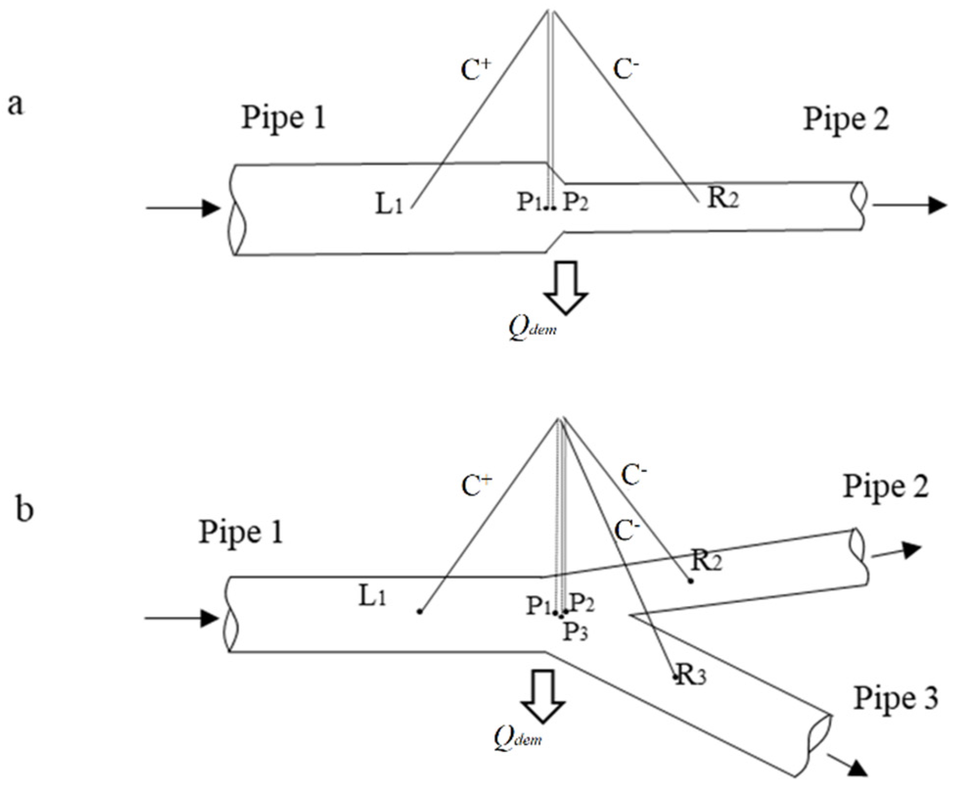
The application of the differential equations assumes the boundary conditions described hereafter. The variables V and H are indexed with P_i corresponding to the points, one on each side of the boundary section, which is nearly superposed (Figure 2). For all the other parameters, only the number of pipes is used as an index to prevent any complication in naming. In both cases of upstream and downstream end boundaries of the systems, only one point exists following C⁻ and C⁺, respectively.

2.3. The Boundary Conditions

The boundary conditions at each end of the pipes describe externally imposed conditions on velocity and/or pressure head. The used and the common ones are examined hereafter.

The potency of the characteristics method is the adequacy of analyzing each boundary and each conduit section separately along the unsteady flow time occurrence.

The boundary conditions described below were considered.

2.3.1. Reservoir

If a reservoir with constant pressure head ${\mathrm{H}}_0$ is located upstream of the network, then:

$${\mathrm{H}}_{{\mathrm{P}}_1}={\mathrm{H}}_0$$

(12)

2.3.2. Valve

Being located at the downstream end of the pipes, the valve closure is assumed to induce a linear flow velocity variation at the cross-section according to the following equation:

$${\mathrm{V}}_{{\mathrm{P}}_1}={\mathrm{V}}_0\times (1-\frac{\mathrm{t}}{{\mathrm{T}}_{\mathrm{c}}})$$

(13)

where V₀ (ms⁻¹) is the initial flow velocity and T_c (s) is the valve closure time.

In the case of a sudden closure (T_c = 0), ${\mathrm{V}}_{{\mathrm{P}}_1}$ becomes equal to zero directly after the perturbation creation.

A detailed analysis with different gate-valves’ closing time (from Tc = 0 to Tc = 6 s) was carried out and published in a previous study by the same authors [3]. The sudden closure was considered to clearly show the effect of the phenomenon.

2.3.3. Internal Boundary Conditions

Junctions with two and three pipes are considered:

1. Two-pipe junction:

A two-pipe junction is shown in Figure 2a.

In the case of no external demand, the values of the four unknowns can be found by solving the set of equations below:

• Following the C⁺ equation (Equation (5)):

  $${\mathrm{V}}_{{\mathrm{P}}_1}=({\mathrm{V}}_{{\mathrm{L}}_1}+\frac{\mathrm{g}}{{\mathrm{a}}_1}{\mathrm{H}}_{{\mathrm{L}}_1}-\frac{{\mathrm{f}}_1\Delta \mathrm{t}}{2{\mathrm{D}}_1}{\mathrm{V}}_{{\mathrm{L}}_1}\left|{\mathrm{V}}_{{\mathrm{L}}_1}\right|)-(\frac{\mathrm{g}}{{\mathrm{a}}_1}){\mathrm{H}}_{{\mathrm{P}}_1}$$

  (14)
• Following the C⁻ equation (Equation (6)):

  $${\mathrm{V}}_{{\mathrm{P}}_2}=\left({\mathrm{V}}_{{\mathrm{R}}_2}-\frac{\mathrm{g}}{{\mathrm{a}}_2}{\mathrm{H}}_{{\mathrm{R}}_2}-\frac{{\mathrm{f}}_2\Delta \mathrm{t}}{2{\mathrm{D}}_2}{\mathrm{V}}_{{\mathrm{R}}_2}\left|{\mathrm{V}}_{{\mathrm{R}}_2}\right|\right)+(\frac{\mathrm{g}}{{\mathrm{a}}_2}){\mathrm{H}}_{{\mathrm{P}}_2}$$

  (15)
• The conservation of mass equation:

  $${\mathrm{V}}_{{\mathrm{P}}_1}{\mathrm{A}}_1={\mathrm{V}}_{{\mathrm{P}}_2}{\mathrm{A}}_2$$

  (16)
• The energy equation at the points P₁ and P₂, neglecting the difference in velocity heads and any local losses:

  $${\mathrm{H}}_{{\mathrm{P}}_1}={\mathrm{H}}_{{\mathrm{P}}_2}$$

  (17)

Solving the above system of equations, the head value H at the junction can be calculated as follows:

$${\mathrm{H}}_{{\mathrm{P}}_1}={\mathrm{H}}_{{\mathrm{P}}_2}=\frac{{\mathrm{C}}_3{\mathrm{A}}_1-{\mathrm{C}}_1{\mathrm{A}}_2}{{\mathrm{C}}_2{\mathrm{A}}_2+{\mathrm{C}}_4{\mathrm{A}}_1}$$

(18)

where ${\mathrm{C}}_1$, ${\mathrm{C}}_2$, ${\mathrm{C}}_3$ and ${\mathrm{C}}_4$ are the function of the known values obtained from the earlier time. By means of a back-substitution, also the flow velocities can be found.

In the case of a series of two pipes with an external constant demand ${\mathrm{Q}}_{\mathrm{dem}}$ (m³ s⁻¹) (that is delivered by one hydrant), a similar system of equations can be used, modifying Equation (16) only, as follows:

$${\mathrm{V}}_{{\mathrm{P}}_1}{\mathrm{A}}_1={\mathrm{V}}_{{\mathrm{P}}_2}{\mathrm{A}}_2+{\mathrm{Q}}_{\mathrm{dem}}$$

(19)

which makes Equation (18) become:

$${\mathrm{H}}_{{\mathrm{P}}_1}={\mathrm{H}}_{{\mathrm{P}}_2}=\frac{{\mathrm{C}}_3{\mathrm{A}}_1-{\mathrm{C}}_1{\mathrm{A}}_2-{\mathrm{Q}}_{\mathrm{dem}}}{{\mathrm{C}}_2{\mathrm{A}}_2+{\mathrm{C}}_4{\mathrm{A}}_1}$$

(20)

2. Three-pipe junction

A three-pipe junction is shown in Figure 2b.

In the case of a pipe junction with one inflow and two outflows, the following equations are used to find the six unknowns:

$$\mathrm{Pipe}1,{\mathrm{C}}^{+}:{\mathrm{V}}_{{\mathrm{P}}_1}={\mathrm{C}}_1-{\mathrm{C}}_2{\mathrm{H}}_{{\mathrm{P}}_1}$$

(21)

$$\mathrm{Pipe}2,{\mathrm{C}}^{-}:{\mathrm{V}}_{{\mathrm{P}}_2}={\mathrm{C}}_3+{\mathrm{C}}_4{\mathrm{H}}_{{\mathrm{P}}_2}$$

(22)

$$\mathrm{Pipe}3,{\mathrm{C}}^{-}:{\mathrm{V}}_{{\mathrm{P}}_3}={\mathrm{C}}_5+{\mathrm{C}}_6{\mathrm{H}}_{{\mathrm{P}}_3}$$

(23)

$$\mathrm{Conservation}\mathrm{of}\mathrm{mass}:{\mathrm{V}}_{{\mathrm{P}}_1}{\mathrm{A}}_1={\mathrm{V}}_{{\mathrm{P}}_2}{\mathrm{A}}_2+{\mathrm{V}}_{{\mathrm{P}}_3}{\mathrm{A}}_3$$

(24)

$$\mathrm{The}\mathrm{energy}\mathrm{balance},\mathrm{neglecting}\mathrm{local}\mathrm{losses}\mathrm{between}1\mathrm{and}2:{\mathrm{H}}_{{\mathrm{P}}_1}={\mathrm{H}}_{{\mathrm{P}}_2}$$

(25)

$$\mathrm{The}\mathrm{energy}\mathrm{balance},\mathrm{neglecting}\mathrm{local}\mathrm{losses}\mathrm{between}1\mathrm{and}3:{\mathrm{H}}_{{\mathrm{P}}_1}={\mathrm{H}}_{{\mathrm{P}}_3}$$

(26)

Solving the previous set of equations leads to:

$${\mathrm{H}}_{{\mathrm{P}}_1}={\mathrm{H}}_{{\mathrm{P}}_2}={\mathrm{H}}_{{\mathrm{P}}_3}=\frac{{\mathrm{C}}_1{\mathrm{A}}_1-{\mathrm{C}}_3{\mathrm{A}}_2-{\mathrm{C}}_5{\mathrm{A}}_3}{{\mathrm{C}}_2{\mathrm{A}}_1+{\mathrm{C}}_4{\mathrm{A}}_2+{\mathrm{C}}_6{\mathrm{A}}_3}$$

(27)

In the case of a three-pipe junction with an outlet, in the previous set of equations, only Equation (24) has to be modified, as follows:

$${\mathrm{V}}_{{\mathrm{P}}_1}{\mathrm{A}}_1={\mathrm{V}}_{{\mathrm{P}}_2}{\mathrm{A}}_2+{\mathrm{V}}_{{\mathrm{P}}_3}{\mathrm{A}}_3+{\mathrm{Q}}_{\mathrm{dem}}$$

(28)

while Equation (27) becomes:

$${\mathrm{H}}_{{\mathrm{P}}_1}={\mathrm{H}}_{{\mathrm{P}}_2}={\mathrm{H}}_{{\mathrm{P}}_3}=\frac{{\mathrm{C}}_1{\mathrm{A}}_1-{\mathrm{C}}_3{\mathrm{A}}_2-{\mathrm{C}}_5{\mathrm{A}}_3-{\mathrm{Q}}_{\mathrm{dem}}}{{\mathrm{C}}_2{\mathrm{A}}_1+{\mathrm{C}}_4{\mathrm{A}}_2+{\mathrm{C}}_6{\mathrm{A}}_3}$$

(29)

2.4. Calculation Process

In order to define the initial conditions for the unsteady flow analysis, a steady-state simulation was executed for each configuration. Starting from the upstream reservoir water level, by substituting the head losses calculated using the Darcy–Weisbach equation, the piezometric elevation (H) and the velocity (V) are defined in each section of the system.

Starting with the pre-computed H and V (calculated from the steady-state conditions), calculations of the new values H_Pn and V_Pn are carried out for each grid point with an increment of ΔT (Figure 1). Therefore, new values of H and V are obtained, and they replace the previous ones. The process continues for the pre-fixed simulation time. The software selects the maximum and the minimum pressure occurring at each section through the time of simulation (selection through time). A second selection through the pipe sections for P_max and P_min is performed (selection through space). The analysis results are tabulated as the maximum and minimum pressure head occurred for each pipe, which will be the basis of the calculation of the indicators.

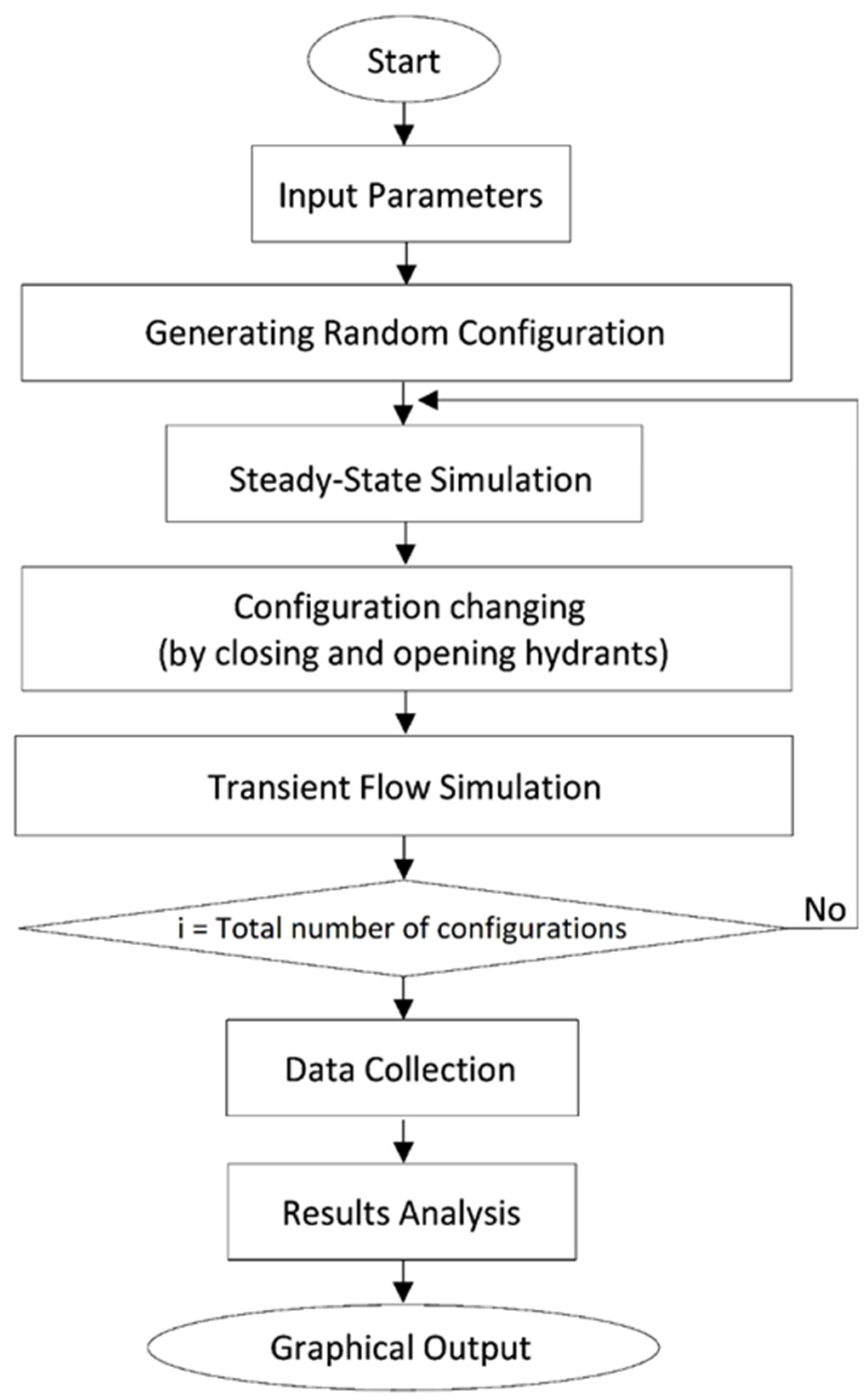
As it was mentioned before, in this study T_max has been chosen to be equal to 30 s, where the water hammer magnitude variation was no more significant. The calculation process is summarized in the flow chart of the software (Figure 3).

2.5. The Hydrant Risk Indicator (HRI)

By analyzing the impacts of different configurations on the hydraulic behavior of the irrigation system, the hydrant risk indicator evaluates the sensitivity of the network in terms of pressure to each hydrant manipulation. It is defined as the ratio between the participation of the hydrant in the riskiest configurations and its total number of participations.

A chosen percentage of the riskiest configurations will yield an upper and lower pressure envelope. The upper envelope represents the maximum pressure magnitude recorded through all the pipes, while the lower envelope represents the minimum recorded pressure magnitude values.

The HRI reflects the potential risk created by each hydrant. Hydrants significantly impacting the overall performance in terms of pressure are expected to appear more frequently in the risky configurations.

$$\mathrm{HRI}=\frac{\mathrm{RPN}}{\mathrm{TPN}}$$

(30)

where TPN is the total participation number, and RPN is the risky participation number. A hydrant will be considered when it is being closed or opened, which is the main reason for the perturbation.

Knowing that the maximum and the minimum pressures are separately treated and presented:

• The HRI_Pmin indicates the ability of each hydrant to create a negative wave (P_min). RPN takes into consideration only the opening mode.
• The HRI_Pmax indicates the ability of each hydrant to create a positive wave (P_max). RPN takes into consideration the closing mode.

It is worth mentioning that the total number of configurations has to be taken to ensure that the indicator achieves the stabilization stage, as explained hereafter. The developed software does not identify the configuration as riskiest, it only identifies the probability of risk.

2.6. Relative Pressure Exceedance (RPE)

This numerically represents the pressure variation and the created risk with respect to the nominal pressure. The RPE was introduced to help both the designer and manager analyze the irrigation systems operating on-demand and illustrate the weak points of the system where any pipe damage may occur. The RPE is defined by:

$$\mathrm{RPE}=100\times \frac{{\mathrm{P}}_{\max }-\mathrm{NP}}{\mathrm{NP}}$$

(31)

The RPE is the relative pressure exceedance (percentage), P_max (bar) is the maximum pressure recorded throughout the simulation time at each section, and NP (bar) is the nominal pressure. In the present study, NP was assumed equal 10 bars for a possible representation of the indicator. The RPE is presented as 10% equiprobability curves, where each curve represents a probability of occurrence.

The user introduces a percentage in the model that represents an envelope percentage of the considered risky for the system (depends on the sensitivity of the network and the norms chosen by the designer and/or the manager). After simulating the different configurations, the model selects the participation of each hydrant in that envelope and translate it to the indicator called Hydrant Risk Indicator.

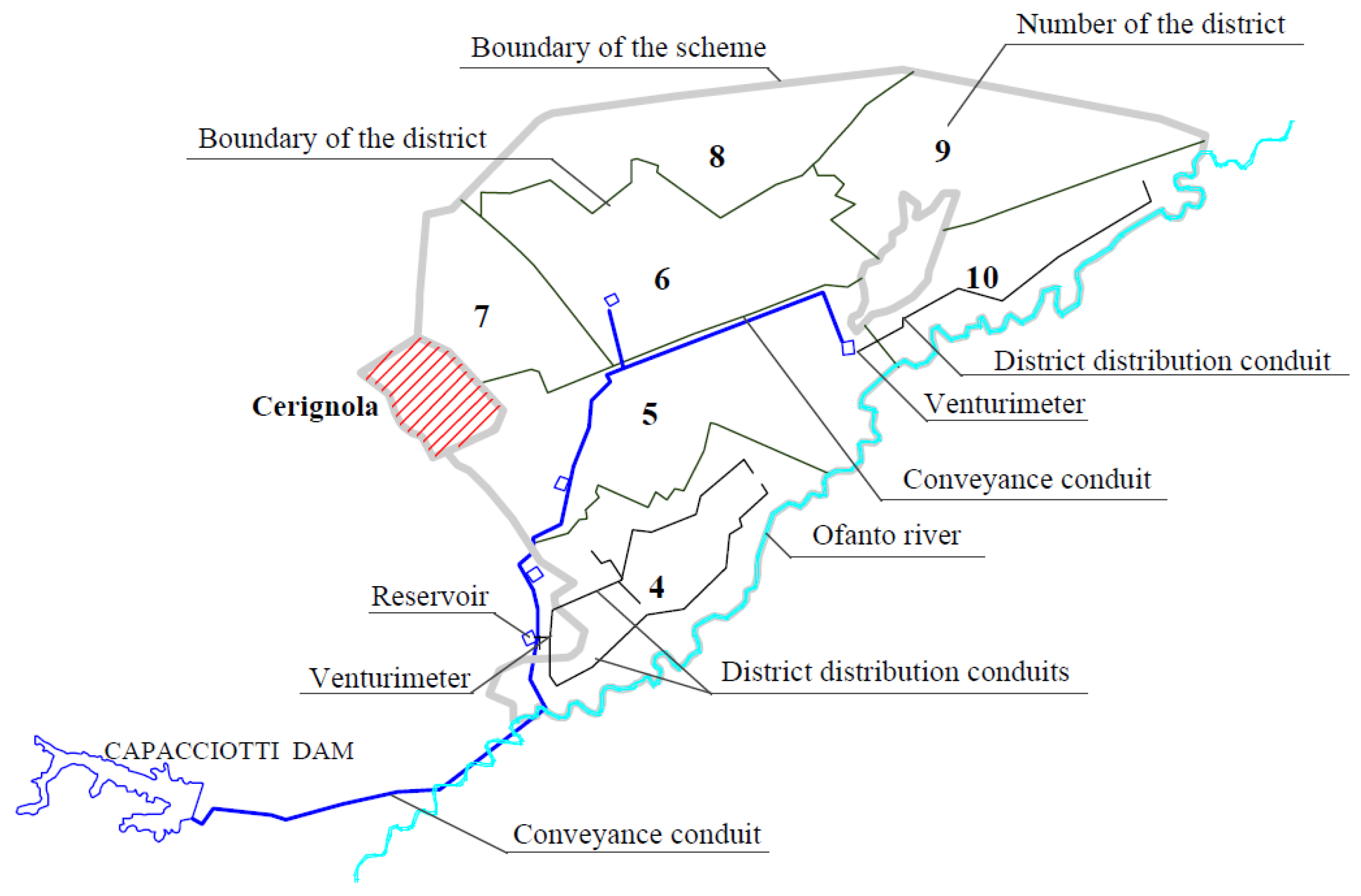
3. The Case Study

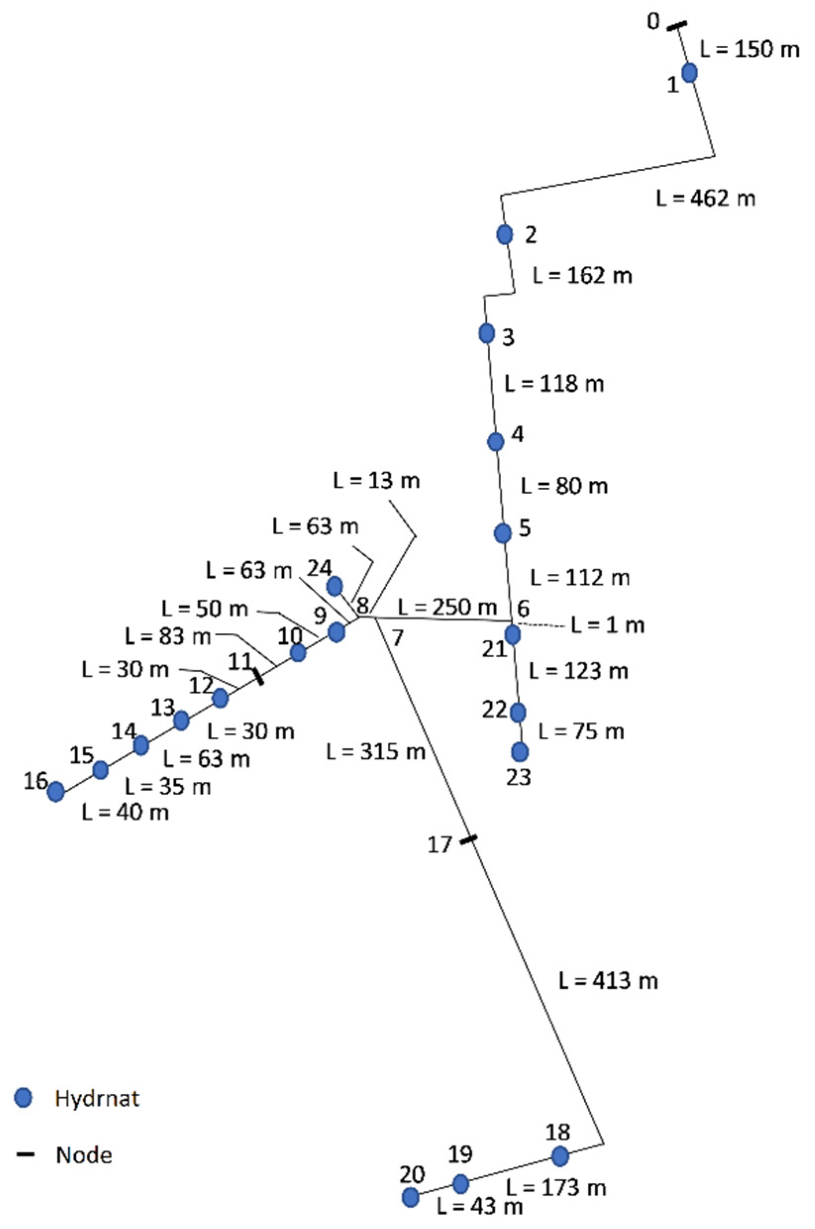
The Sinistra Ofanto irrigation scheme, in the province of Foggia (Italy), is divided into seven irrigation districts (Figure 4). District four, in turn, is subdivided into sectors. The study was performed for the sector 25. The irrigation network is an on-demand pressurized irrigation system. It consists of 19 hydrants with a nominal discharge of 10 (L s⁻¹) and an upstream end constant piezometric elevation of 128 m a.s.l. The NP was equal to 10 bars for all installed pipes, as per the information obtained from the managers. The layout of sector 25 is reported in Figure 5.

With an irrigation network of 19 hydrants and four possible operating modes for each of them (open, closed, opening and closing), an enormous number of configurations could be generated, assuming that the network has been designed as having five hydrants simultaneously open. The selection of a rather small system fulfills the objective of clarity and simplification of the comparison between the results, and makes it possible to analyze different configurations of hydrants. Nonetheless, the code supports large-scale networks and the desired combination of hydrants.

The transient flow is defined as the transition from one steady flow to another steady flow. To keep the assumption of having five hydrants simultaneously open, the perturbation in the present study was created by closing two hydrants and substituting them by opening two new ones.

4. Results and Discussion

4.1. The Uniformity of Random Generated Configurations

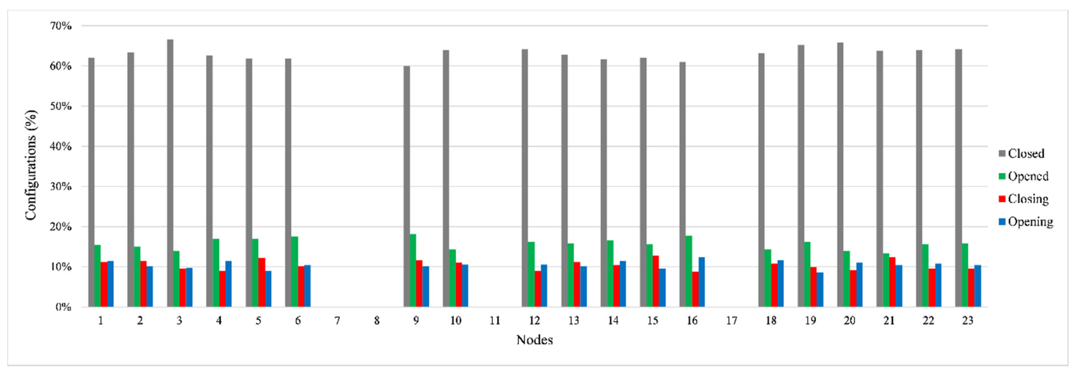
The strong variation of the discharges flowing into the network due to the variation in the demand is the first provoker of perturbation in pressurized irrigation systems. That variation was presented through different configurations. With a view to having a good representation, the software used a random number generator to run different configurations following a uniform distribution function (having the same possibility of getting one operating mode for each hydrant), as shown in Figure 6. The reported results refer to the opening/closing of two hydrants, as this situation occurs with a higher probability compared to the simultaneous opening/closing of three, four or five hydrants, and stronger waves with respect to the opening/closing of one hydrant do occur.

4.2. Computation of the Unsteady Flow Pressure Envelopes

In this study, the hydrant closing time Tc = 0 was considered, as it represented the riskiest case that may happen.

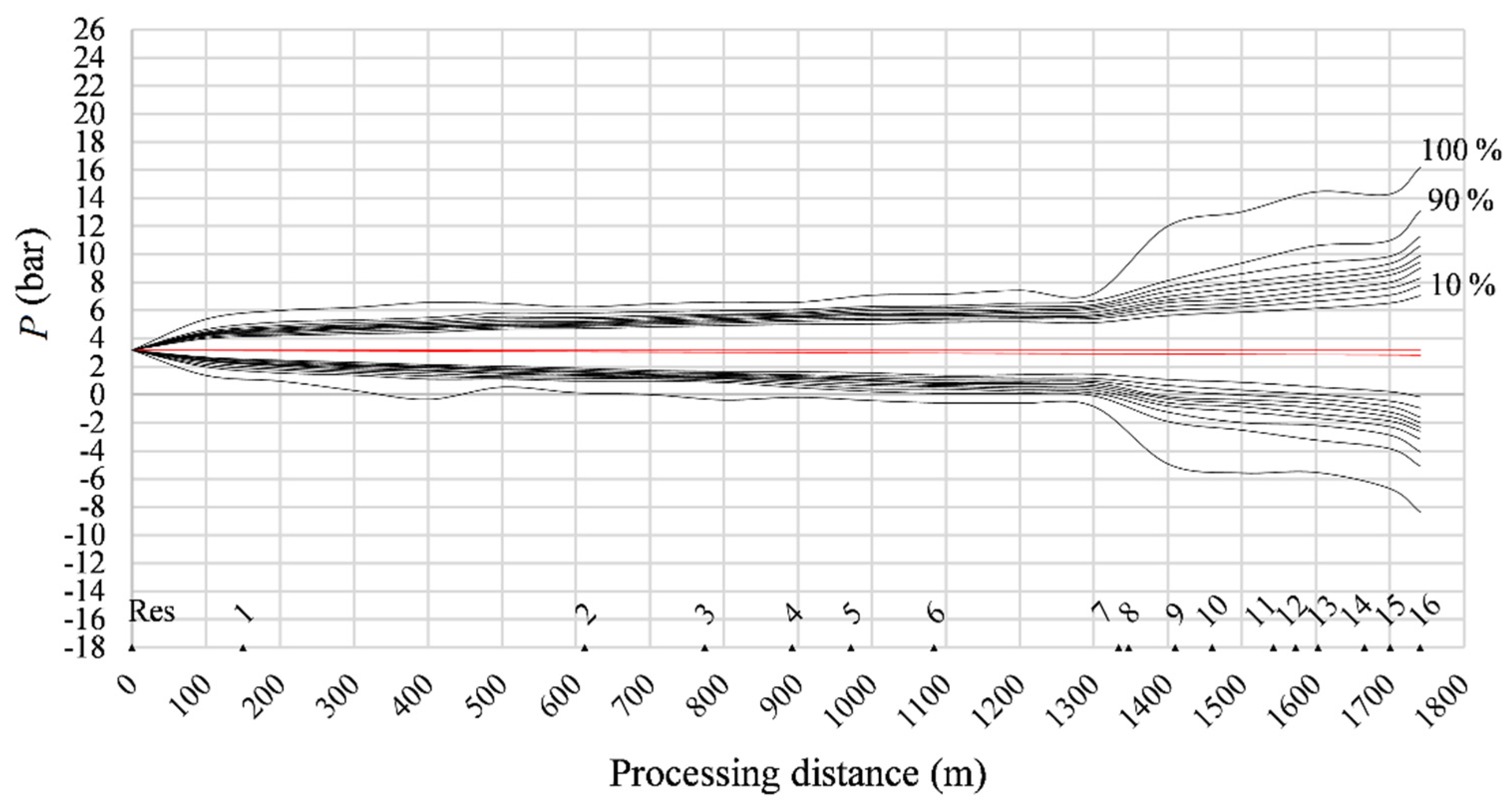
The irrigations system consisted of four layout profiles; only the calculated pressures for the profile Res-Node 16 are presented in Figure 7. After the perturbation, the maximum and the minimum pressure waves were recorded along the pipes and presented as 10% equiprobability curves.

Figure 7 shows that the maximum pressure variation for the different steady-state conditions. At node 16, this was around 0.35 bar (red lines) and increased when moving from the upstream end of the studied profile to downstream.

It is worth mentioning that the code imposed a constraint of not having the water column separation, even with the occurrence of low pressure, in line with the assumption mentioned above, that the pipes were assumed to be full and remained full during the transient flow occurrence, which enabled the application of the differential equations.

4.3. Calculation of the HRI

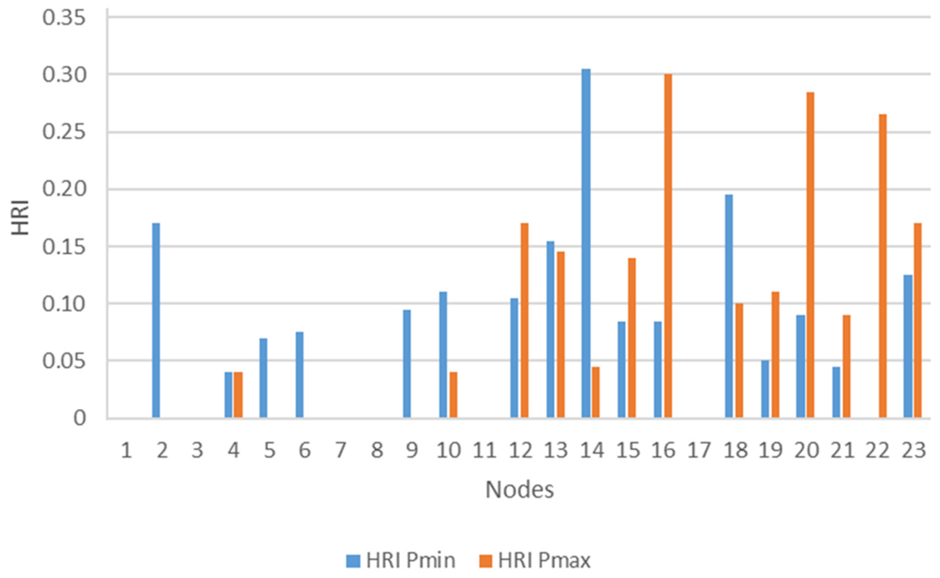
To assess the network response to the different perturbations of configurations, 500 different configurations were generated and analyzed. The number of configurations was run not only to satisfy the uniformity test, but also for the stability of the new indicator. In fact, the HRI graph started to take its final shape at around 350 configurations, where only the real risky hydrants appeared. Once the values were stabilized, the increase in the number of configurations did not significantly affect the results (Figure 8, Figure 9 and Figure 10).

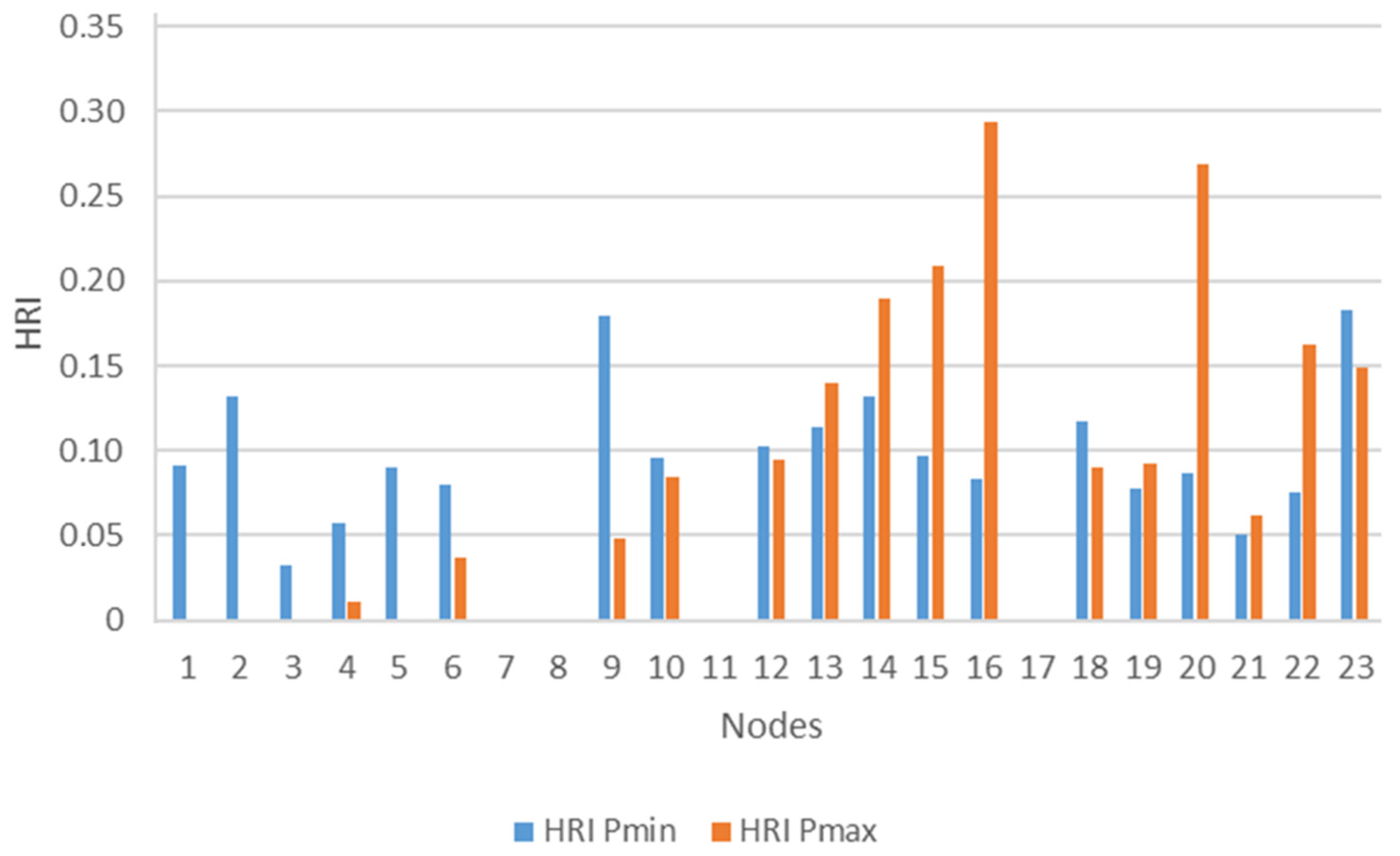
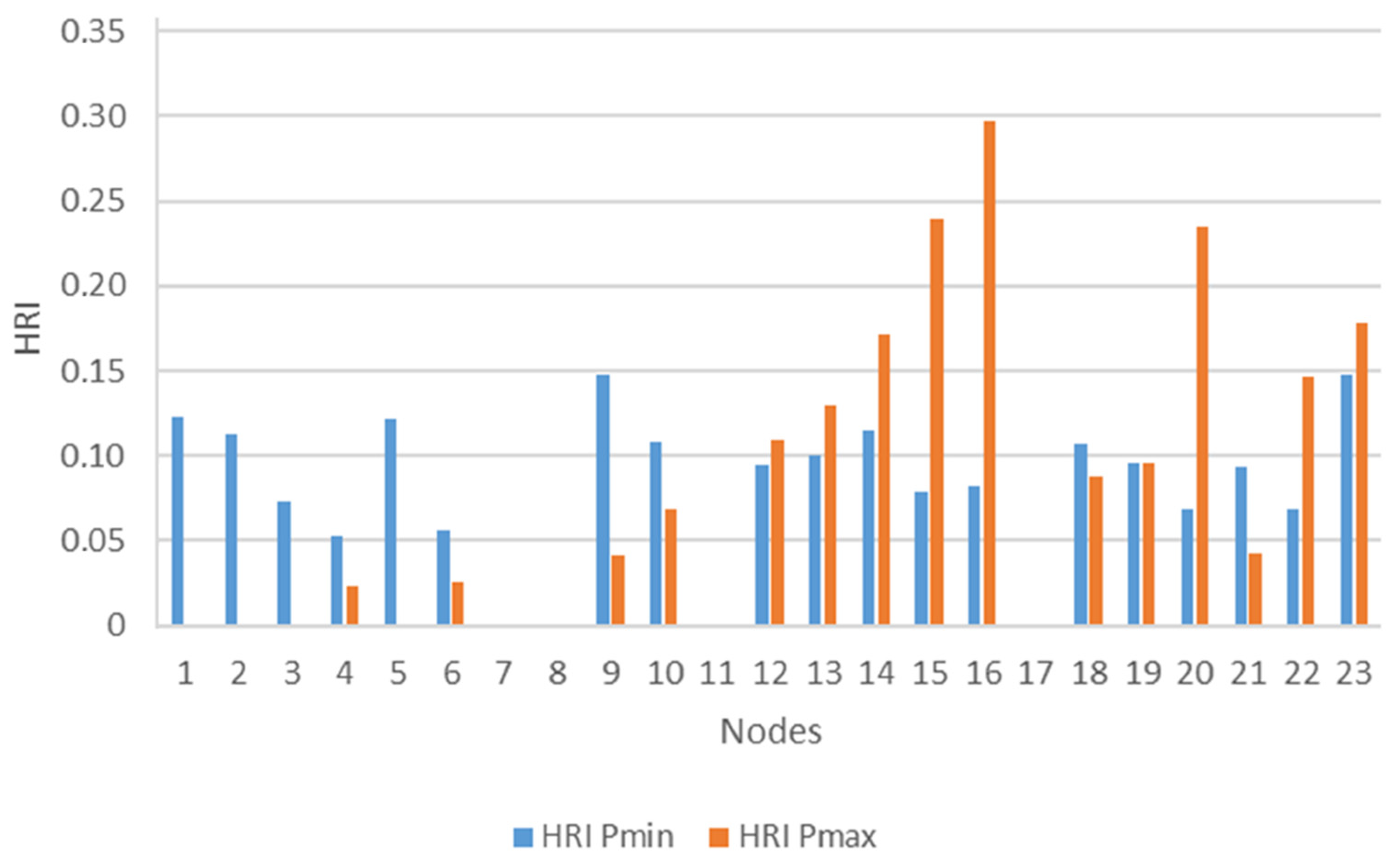
By running 500 configurations for the allocated system, where all nodes were represented, the contribution of the riskiest hydrants could be easily identified by noticing the extreme irregularities of the generated graphs (Figure 10). In the presented case, hydrants 14, 15, 16 and 20 could be identified as risky hydrants, which could generate positive pressure waves.

The term “risky configuration” could be precisely defined, in this case, as the configuration, which caused an exceedance of the allowed domain of the variation in pressure set by the manager according to certain criteria (mainly the system infrastructure).

In these extreme cases, risky hydrants had a high probability to cause either positive or negative waves. The impacts of such cases could cause serious problems.

4.4. Calculation of the RPE

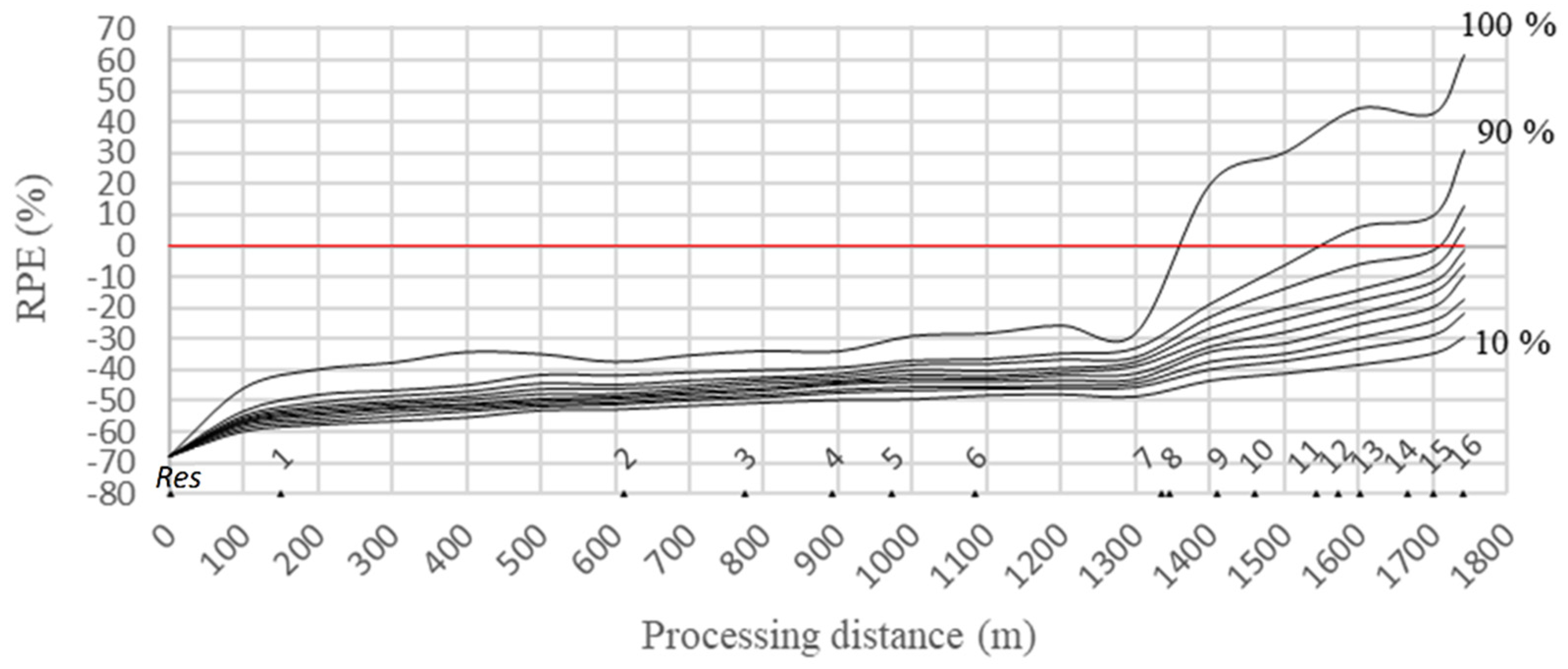
The RPE provides a very clear idea about the pipes under risk (P_max influence). The pipes are considered to be safe when the RPE values are negative, which means that the maximum occurred pressure does not exceed the nominal pressure. As a value of zero means that the transient pressure is equal to the nominal pressure, from that value onwards the pipes start being under risk.

In Figure 11, the pipes for the main line (Res-Node 8) were in the safe range (RPE < 0). At the level of the node 8, which is the entrance of the branch 8–16, the RPE started to take positive values with less than a 10% probability of occurrence. The zone corresponding to the hydrants from 11 to 13 were potentially subject to failure with a 10% probability of occurrence. The more distant the section from the upstream end, the greater the risk of pipe failure. The failure reached its maximum occurrence probability of 40% (100 − 60%) at the downstream end of the layout profiles (hydrant 16).

In parallel with the probability of occurrence and the corresponding zones, it is important to mention the role of the RPE that provides an overview of the exceedance severity.

5. Conclusions

The performance of on-demand pressurized irrigation systems is highly affected by unsteady flow, which highlights the importance of identifying appropriate indicators to be integrated into the designing and managing of a pressurized system.

To that end, user-friendly computer code capable of simulating the real operating conditions of a pressurized irrigation system, and consequently, the unsteady flow through the random opening and closing of hydrants was developed. The code made it possible to investigate and quantify the generated effects through two simple indicators developed in the framework of this study (the hydrant risk indicator, or HRI, and the relative pressure exceedance, or RPE).

Such informative indicators could significantly contribute to more efficient operation management of on-demand pressurized systems by avoiding highly risky probabilistic configurations. Moreover, they could be embedded in the designing phase, allowing for a better interpretation of the impacts of different design alternatives.

References

- Lamaddalena, N.; Sagardoy, J.A. Performance Analysis of On-Demand Pressurized Irrigation Systems; Food and Agriculture Organization: Roma, Italy, 2000; Volume 59. [Google Scholar]
- Calejo, M.; Lamaddalena, N.; Teixeira, J.; Pereira, L. Performance analysis of pressurized irrigation systems operating on-demand using flow-driven simulation models. Agric. Water Manag. 2008, 95, 154–162. [Google Scholar] [CrossRef]
- Lamaddalena, N.; Khadra, R.; Derardja, B.; Fratino, U. A New Indicator for Unsteady Flow Analysis in Pressurized Irrigation Systems. Water Resour. Manag. 2018, 32, 3219–3232. [Google Scholar] [CrossRef]
- Clemmens, A.J. Improving irrigated agriculture performance through an understanding of the water delivery process. J. Irrig. Drain. 2006, 55, 223–234. [Google Scholar] [CrossRef]
- Playán, E.; Mateos, L. Modernization and optimization of irrigation systems to increase water productivity. Agric. Water Manag. 2006, 80, 100–116. [Google Scholar] [CrossRef] [Green Version]
- Renault, D.; Facon, T.; Wahaj, R. Modernizing Irrigation Management: The MASSCOTE Approach--Mapping System and Services for Canal Operation Techniques; Food and Agriculture Organization: Roma, Italy, 2007; Volume 63. [Google Scholar]
- Abuiziah, I.; Oulhaj, A.; Sebari, K.; Ouazar, D.; Saber, A. Simulating Flow Transients in Conveying Pipeline Systems by Rigid Column and Full Elastic Methods: Pump Combined with Air Chamber. Eng. Technol. Int. J. Mech. Aerosp. Ind. Mechatron. Manuf. Eng. 2013, 7, 2391–2397. [Google Scholar]
- Wichowski, R. Hydraulic transients analysis in pipe networks by the method of characteristics (MOC). Arch. Hydro-Eng. Environ. Mech. 2006, 53, 267–291. [Google Scholar]
- Bergant, A.; Tijsseling, A.S.; Vítkovský, J.P.; Covas, D.I.; Simpson, A.R.; Lambert, M.F. Parameters affecting water-hammer wave attenuation, shape and timing—Part 1: Mathematical tools. J. Hydraul. Res. 2008, 46, 373–381. [Google Scholar] [CrossRef] [Green Version]
- Wylie, E.B.; Streeter, V.L.; Suo, L. Fluid Transients in Systems; Prentice Hall: Englewood Cliffs, NJ, USA, 1993; Volume 1. [Google Scholar]
- Chaudhry, M.H. Applied Hydraulic Transients; Springer: Berlin/Heidelberg, Germany, 1979. [Google Scholar]
- Larock, B.E.; Jeppson, R.W.; Watters, G.Z. Hydraulics of Pipeline Systems; CRC Press: Boca Raton, FL, USA, 1999. [Google Scholar]
- Chaudhry, M.H. Transient-flow equations. In Applied Hydraulic Transients; Springer: Berlin/Heidelberg, Germany, 2014; pp. 35–64. [Google Scholar]
- Lamaddalena, N.; Pereira, L.S. Pressure-driven modeling for performance analysis of irrigation systems operating on demand. Agric. Water Manag. 2007, 90, 36–44. [Google Scholar] [CrossRef]
Figure 1.
Characteristic curves on the space–time plane.
Figure 2.
Boundary conditions at a typical series of (a) two and (b) three pipes junction.
Figure 3.
Computer code flowchart.
Figure 4.
The Sinistra Ofanto irrigation scheme.
Figure 5.
Layout of the network (sector 25).
Figure 6.
Uniformity distribution of the random number generator (500 hydrant configurations).
Figure 7.
Pressure profile (Res-node 16) for 500 configurations, considering the simultaneous opening and closing of two different hydrants out of five.
Figure 8.
Hydrant risk indicator (HRI) for 50 configurations.
Figure 9.
Hydrant risk indicator (HRI) for 350 configurations.
Figure 10.
Hydrant risk indicator (HRI) for 500 configurations.
Figure 11.
Relative pressure exceedance (RPE) for 500 configurations.
© 2019 by the authors. Licensee MDPI, Basel, Switzerland. This article is an open access article distributed under the terms and conditions of the Creative Commons Attribution (CC BY) license (http://creativecommons.org/licenses/by/4.0/).
Share and Cite
MDPI and ACS Style
Derardja, B.; Lamaddalena, N.; Fratino, U. Perturbation Indicators for On-Demand Pressurized Irrigation Systems. Water 2019, 11, 558. https://doi.org/10.3390/w11030558
AMA Style
Derardja B, Lamaddalena N, Fratino U. Perturbation Indicators for On-Demand Pressurized Irrigation Systems. Water. 2019; 11(3):558. https://doi.org/10.3390/w11030558
Chicago/Turabian StyleDerardja, Bilal, Nicola Lamaddalena, and Umberto Fratino. 2019. "Perturbation Indicators for On-Demand Pressurized Irrigation Systems" Water 11, no. 3: 558. https://doi.org/10.3390/w11030558
Note that from the first issue of 2016, this journal uses article numbers instead of page numbers. See further details here.