Assessment of Water Quality Parameters Using Temporal Remote Sensing Spectral Reflectance in Arid Environments, Saudi Arabia


1
Department of Hydrology and Water Resources Management, Faculty of Meteorology, Environment & Arid Land Agriculture, King Abdulaziz University, Jeddah 21589, Saudi Arabia
2
Laboratory of Forest Management and Remote Sensing, School of Forestry and Natural Environment, Aristotle University of Thessaloniki, Thessaloniki 54124, Greece
3
School of Environmental Engineering, Technical University of Crete, Chania 73100, Greece
*
Author to whom correspondence should be addressed.
Water 2019, 11(3), 556; https://doi.org/10.3390/w11030556
Submission received: 16 February 2019
/
Revised: 12 March 2019
/
Accepted: 14 March 2019
/
Published: 17 March 2019
(This article belongs to the Special Issue Catchment Water Resources Management: Advances in Remote Sensing Based Techniques)
Abstract
:Remote sensing applications in water resources management are quite essential in watershed characterization, particularly when mega basins are under investigation. Water quality parameters help in decision making regarding the further use of water based on its quality. Water quality parameters of chlorophyll a concentration, nitrate concentration, and water turbidity were used in the current study to estimate the water quality parameters in the dam lake of Wadi Baysh, Saudi Arabia. Water quality parameters were collected daily over 2 years (2017–2018) from the water treatment station located within the dam vicinity and were correspondingly tested against remotely sensed water quality parameters. Remote sensing data were collected from Sentinel-2 sensor, European Space Agency (ESA) on a satellite temporal resolution basis. Data were pre-processed then processed to estimate the maximum chlorophyll index (MCI), green normalized difference vegetation index (GNDVI) and normalized difference turbidity index (NDTI). Zonal statistics were used to improve the regression analysis between the spatial data estimated from the remote sensing images and the nonspatial data collected from the water treatment plant. Results showed different correlation coefficients between the ground truth collected data and the corresponding indices conducted from remote sensing data. Actual chlorophyll a concentration showed high correlation with estimated MCI mean values with an R2 of 0.96, actual nitrate concentration showed high correlation with the estimated GNDVI mean values with an R2 of 0.94, and the actual water turbidity measurements showed high correlation with the estimated NDTI mean values with an R2 of 0.94. The research findings support the use of remote sensing data of Sentinel-2 to estimate water quality parameters in arid environments.
1. Introduction
There are many changes in the water body that take place when flowing water stops at the lowest elevation point on land. The flowing water transfers and holds the temperature from one location to the next, so all drainages that recharge a natural reservoir or an artificial dam will affect the water at the destination [1]. Moreover, thermal changes in the water body are associated with chemical changes which influence the organism cycle at the lagoon. Again, small streams and other channels that end at a lagoon will carry any small particles in its path and transfer all these pollutants to the lagoon [2]. As the water stays in the dam or in a pond, more recharge streams will contaminate it and move more sediment to the dam. Hence, over a long period, the change in the water quality will be larger than the change within a short time. In the case of water at a dam, all water supplies from that dam will be contaminated [3].
The amount of decline in water quality is connected to the retention time of the dam’s water and its storage capacity in relation to the amount of water charging the dam during the year. Water in a small pond behind a run-of-river dam will undergo very little or no deterioration; that stored for many months or even years behind a major dam may be lethal to most life in the reservoir and in the river for many kilometers below the dam [4].
Sinking organic materials will consume oxygen in the water. Then, undesirable materials, like carbon dioxide and methane, are released into the dam water. This procedure can take a decade or so, although, in the tropics it may take many decades or even centuries for most of the organic matter to molder [5]. One of the large events that caused great harm to the environment and the surrounding people happened at Brokopondo Dam in 1964.
Normal bacteria can change the water quality because of cyanobacteria concentrations. Cyanobacteria produce a greenish floating matter over the surface of the water body—bloom—which pollutes the water and is associated with respiratory problems and skin irritation issues [6]. Also, a high concentration of such bacteria leading to a slight aberrance in the amount of nitrogen will cause a strong and horrific smell. Discovering harmful blooms over the surface of the water body while in the early stages is very important for protecting the water quality and to control the water source [7].
Digital pictures are easier to use than older images, also, they allow researchers to work with bigger areas than before. In addition, digital images can be saved onto small hard drives and used later with most standard computers carrying the appropriate software. In fact, digital images have opened the doors for many kinds of developments, such as watershed modeling, ship tracking, accurate weather forecasting, flood analyzing, and other beneficial examples of gained knowledge [8]. At the same time, other scientists working on wave bands were trying to study the effects of each band on different objects. Sensors were also developed to detect invisible bands [9].
In recent times, the Environmental Protection Agency (EPA) has been developing and offering an application that monitors the water surface and provides a reasonable water quality parameter and is available for normal users. The current observation application uses satellite data that comes from the European Space Agency (ESA). The ESA gets images and data by using the ocean land color instrument (OCLI), USGS Landsat satellite, and the medium resolution imaging spectrometer (MODIS). Sentinel-2 provides data with a high spatial resolution and has been used in conjunction with developed models to detect chlorophyll and dissolved organic matter. A recent study on Sentinel-2 shows that the most accurate algorithm to acquire the highest reflectance from dissolved organic matter (DOM) comes from bond 5 and bond 3. Bond 4 and 5 were used to develop a model to detect chlorophyll with low root mean squared error [10]. Furthermore, Sentinel-2 with an onboard multispectral imager MSI was proven, in more than one study, to be more accurate than the moderate-resolution imaging spectroradiometer. MSI has been used to detect suspended particulate matter in the water body and its results were acceptable within a wavelength range of 560 to 780 nm [11].
In this study, the goal is to monitor the water quality, therefore, the focus will be on the highest reflectance percentage from the chlorophyll, nitrogen, and water turbidity. Sentinel-2 provides data with high spatial resolution and has developed models for detecting such parameters. Regression analysis is practiced in the current research to define the relationship between the actual and the estimated water quality parameters.
2. Materials and Methods
2.1. Study Area Description
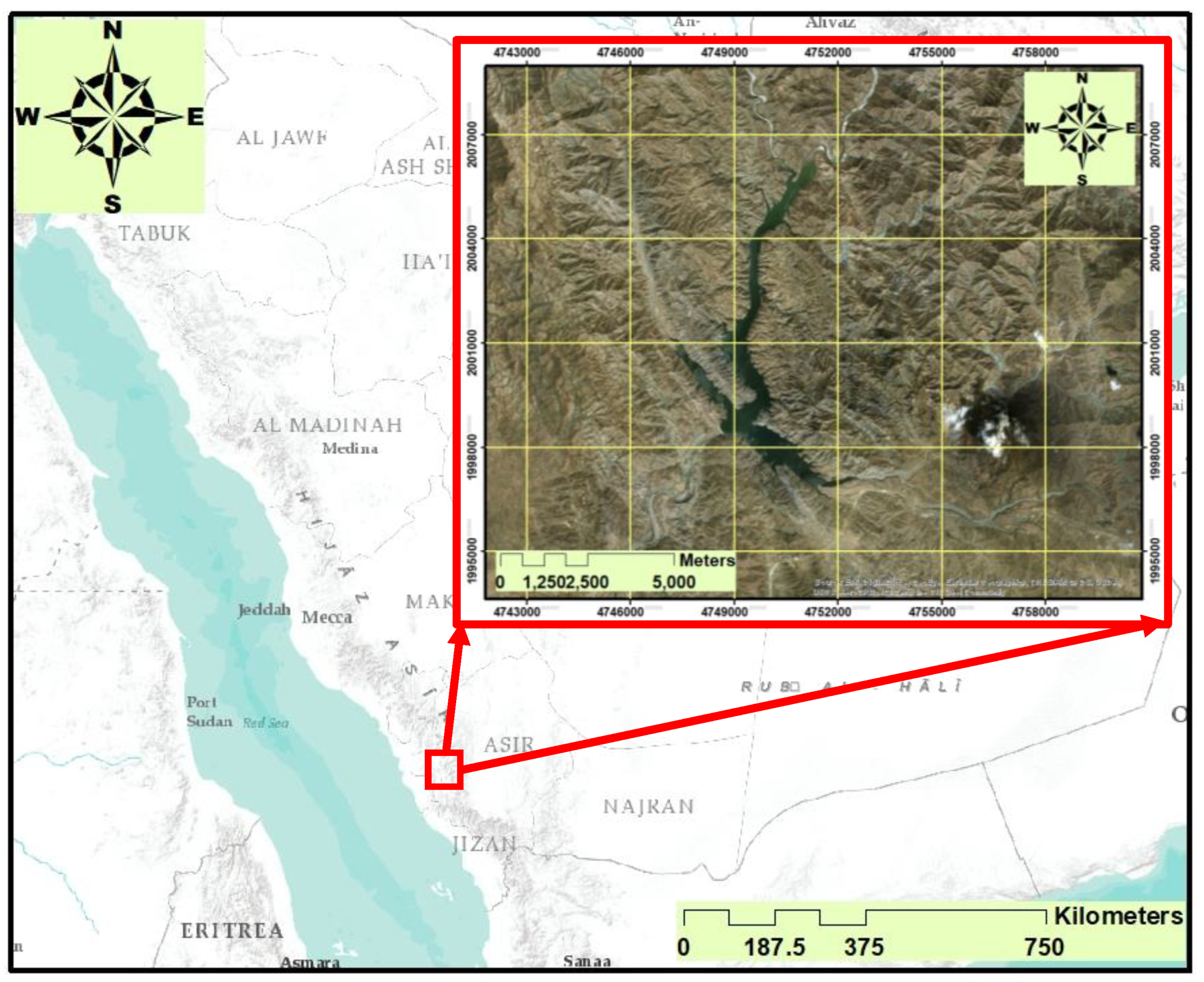
Baysh Dam is a gravity dam on Wadi Baysh around 35 km upper east of Baysh in the Jizan Region of southwestern Saudi Arabia (Figure 1). The dam has numerous reasons to incorporate surge control, water system, and groundwater revive. The Baysh Dam was constructed between 2003 and 2009, and is owned and operated by the Ministry of Water and Electricity. The Baysh Dam is 120 m high from the foundation level, with no sunlight reaching the bottom of the dam’s lake. The total reservoir capacity of the dam is 192 million cubic meters. The dam normally requires a long time to be clear of the effects of organic materials. Sinking organic materials will consume oxygen in the water. Then, undesirable gases, like carbon dioxide and methane, are released into the dam water. This procedure can take a decade or so, although, in the tropics it may take many decades or even centuries for most of the organic matter to molder.
2.2. Water Sample Collection
Regular water sample collections were initiated during the middle of each climatic season. From 2017 to 2018, following the complete random sampling (CRS) technique [12], a total of 120 water samples were collected and transferred to the laboratory to perform the designated colorimetry test [13], nitrate concentration (mg/L) test [14], and turbidity test (NTU) [15]. For the restricted part of the lake, water quality parameters were collected from the water treatment plant located at the vicinity of the dam lake.
2.3. Remote Sensing Data
Routine collection of Sentinel-2 data began in January 2017 and continued until the end of December 2018 on a sensor revisit resolution (16 days) which resulted in total of 52 images. The Sentinel-2 instrument is made of 12 spectral bands with a 10 m resolution of visible bands (VI), 20 m resolution of vegetation red edge (VRE) bands, and short-wave infrared (SWIR) bands, in addition to three bands related to coastal aerosols and water vapor of 60 m resolution. Three different remotely sensed indices were obtained to represent three different water quality parameters, maximum chlorophyll index (MCI), green normalized difference vegetation index (GNDVI), and normalized difference turbidity index (NDTI).
2.3.1. Maximum Chlorophyll Index
Maximum chlorophyll index (MCI) was used to exploit the height of the measurements in a certain spectral band above a baseline which passes through three bands B4 (665 nm), B5 (705 nm), and B6 (740 nm) [16,17]. The MCI for floating vegetation and inland water bodies is estimated using the algorithm of Matthews et al. [18] considering the top of atmosphere (TOA) condition:
where Rrs can be obtained based on a field measurement as follows [19]:
where Rp is the standard reflectance panel, Lw(λ) is the radiance of water-viewing, Lsky(λ) is sky-measured radiance, ρ is the air–water interface reflectance, and Lp is the radiance reference panel.
2.3.2. Green Normalized Difference Vegetation Index
The green normalized difference vegetation index is based on two-band combinations of the red-edge region of the spectrum [20]. GNDVI is very sensitive to the change in chlorophyll content, which is tidally related with the nitrogen content at the dam lake. The nitrogen index was created and found from the following equation [21]:
(NIR − Green)/(NIR + Green).
The normalized difference vegetation index was used to detect nitrogen content using the following equation:
(NIR − (690 nm~710 nm))/(IR + (690 nm~710 nm)).
After many studies, it was found that using the green ray for detection of nitrogen content was more effective than the normal vegetation index. Therefore, GNDVI uses the following equation [22]:
GNDVI = ((NIR − (540 nm~570 nm))/(NIR + (540 nm~570 nm)).
The wavelength which was used in the previous equation was shifted to the green edge in order to get a clearer result from satellite images [22], where NIR is the near-infrared band of Sentinel-2.
2.3.3. Normalized Difference Turbidity Index
Lacaux et al. [23] developed an algorithm to estimate the water turbidity using remote sensing data specifically for ponds and inland waters, and it can be estimated as follows:
where R is the red band of Sentinel-2, and G is the green band of Sentinel-2.
2.4. Data Normalization and Regression Analysis
In order to establish a regression analysis between the actual and estimated water quality parameters, a data normalization procedure is essential task to omit the unit’s dimension from the two datasets. Data normalization can be achieved as follows [24]:
The basic equation for Pearson’s correlation is defined as follows [25]:
where N is number of pairs of scores, ∑xy is sum of the products of paired scores, ∑x is sum of x scores, ∑y is sum of y scores, ∑x2 is sum of squared x scores, and ∑y2 is sum of squared y scores.
The intention behind performing the regression analyses is to envisage the regression potentials between the actual and the remotely sensed estimated water quality parameters. Therefore, the actual parameters will be plotted against the estimated parameters and root mean square error (RMSE) values are used to obtain the best fit. RMSE is obtained as follows [26]:
where P is the predicted value; O is the observed values.
Zonal statistics under arc environment were exercised and resulted in four different statistic types (mean, P 90 “majority”, maximum, and minimum values of the input raster) which were used in the regression analysis to identify the best fit.
3. Results and Discussion
Multiple empirical regression analyses were exercised in order to evaluate and realize the coherent relationships between the actual water quality parameter concentrations collected in situ and the corresponded water quality parameters in reflectance values estimated from remote sensing data.
The in-situ water quality parameters were taken daily by the dam authority for routine analysis, therefore, there was no time difference between the in-situ sampling and remote sensing data acquisition.
Statistical analyses that included calculations of the average, maximum, and minimum values, and linear and nonlinear regressions were performed. Pearson correlation analysis was used to investigate the strength of the association between the two variables with a correlation coefficient (r). Significance levels were reported to be significant (p < 0.05) or not significant (p > 0.05) with a t-test, which provides evidence of an association between the two variables.
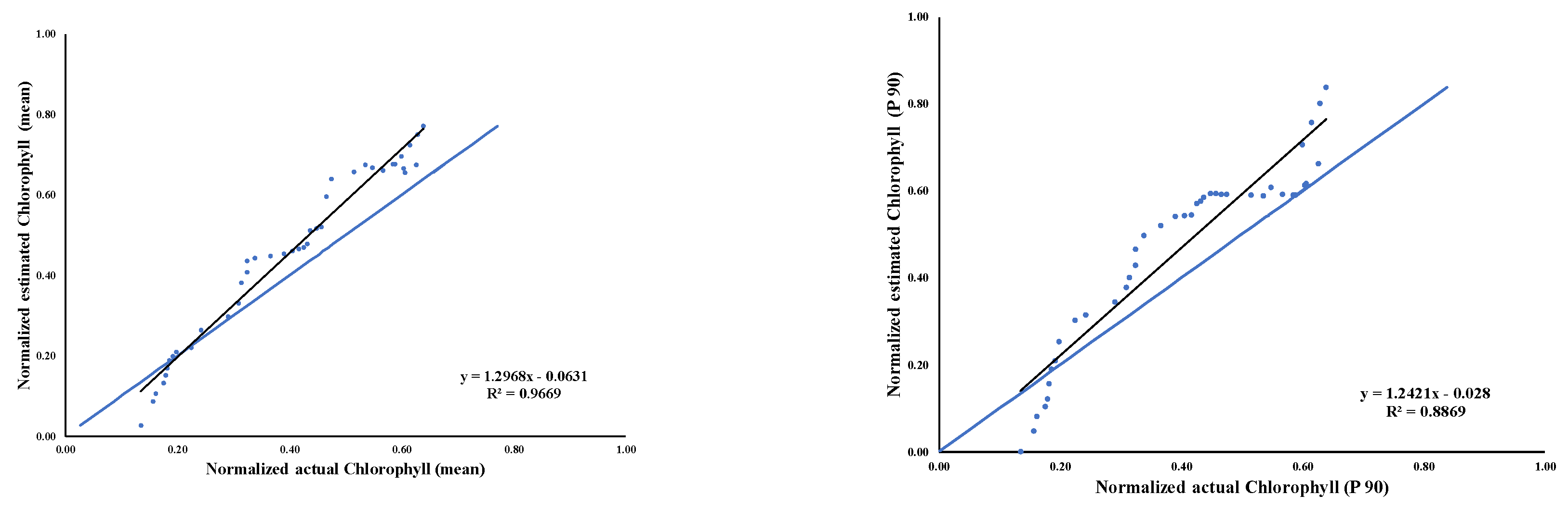
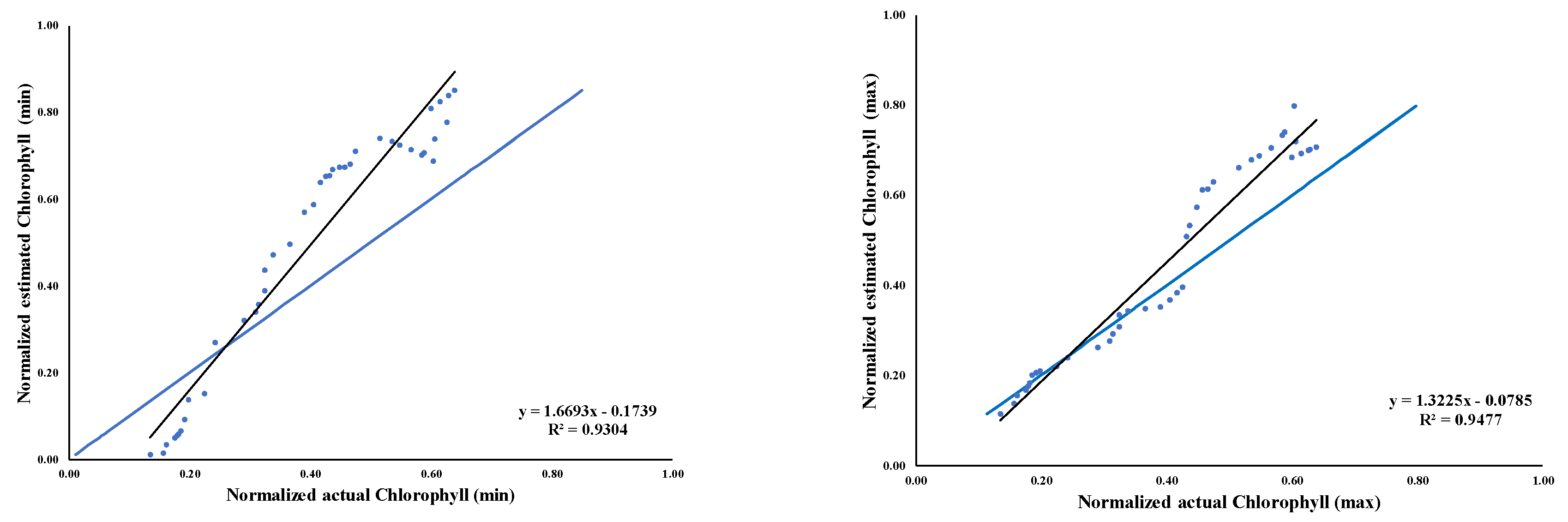
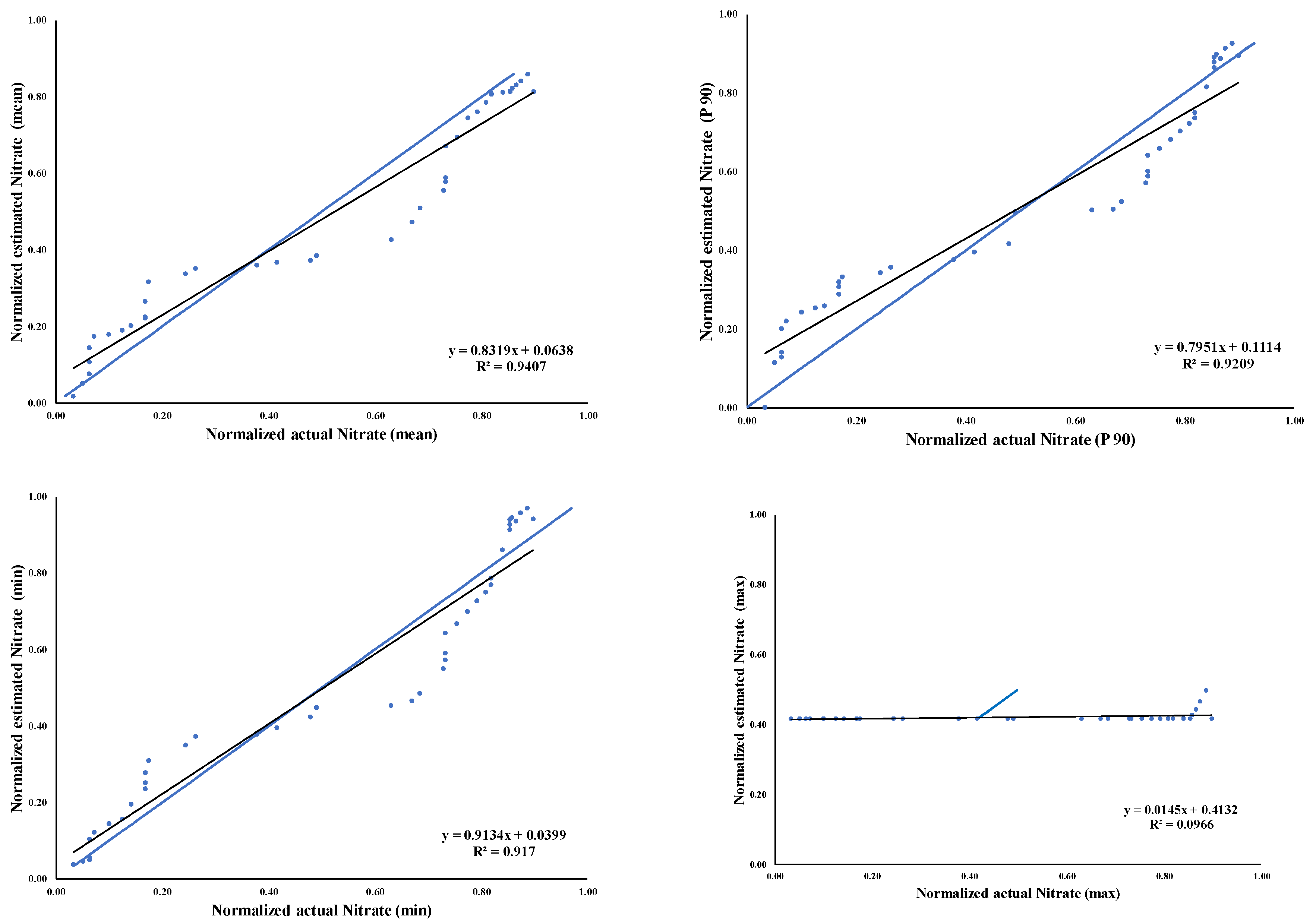
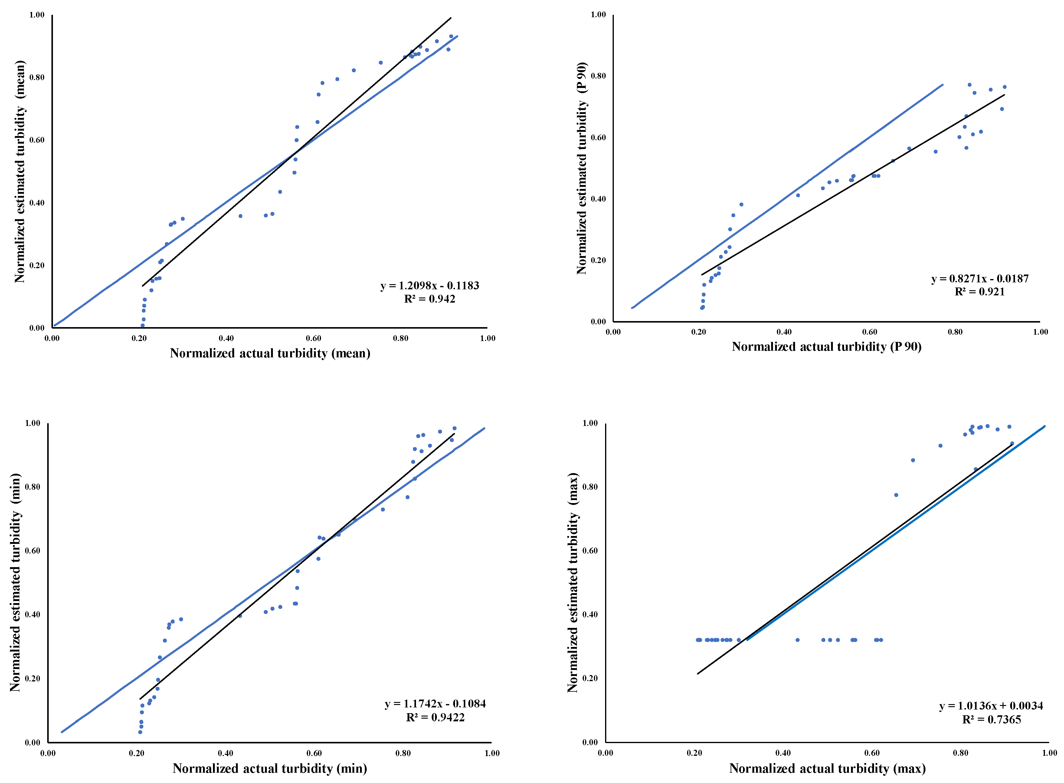
Statistical analyses were performed using the mean values of in situ measurements against the mean, P 90 (majority), maximum, and minimum values of remote sensing data to evaluate the analysis consistencies in linear and nonlinear regressions. The variables’ association strength was examined for subsequent Person correlation with p < 0.05 for a significant association and p > 0.05 for no significant association. Figure 2, Figure 3 and Figure 4 demonstrates the linear regression analysis of MCI, GNDVI, and NDTI, respectively.
Regression results showed that mean pixel values were the best for presenting a coherent association between the actual water parameters and the remotely sensed estimated ones in each of the investigated water quality parameters (MCI, GNDVI, and NDTI). RMSE expressed in Table 1 confirms the robust association between the mean value of the in-situ water quality measurements and the conducted values from remote sensing data based on the summary of the fit analysis [27,28].
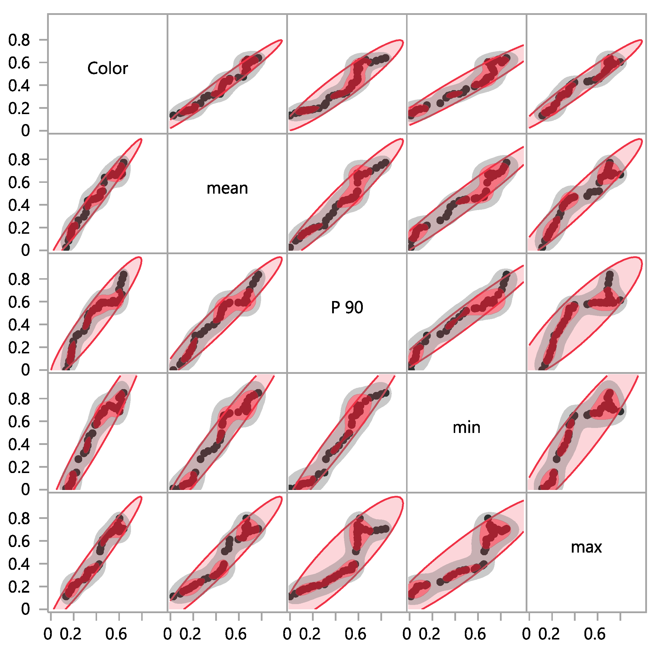
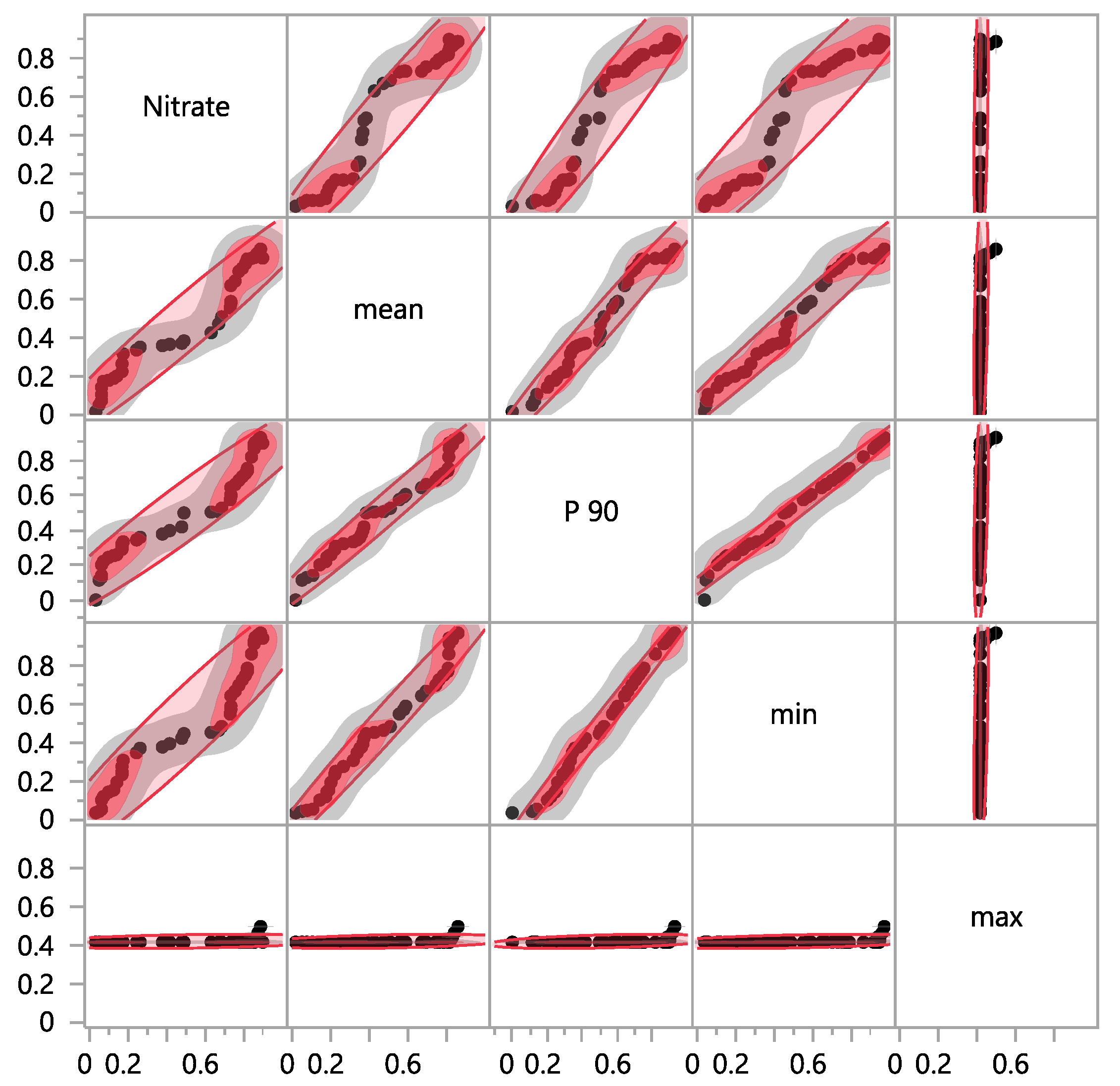
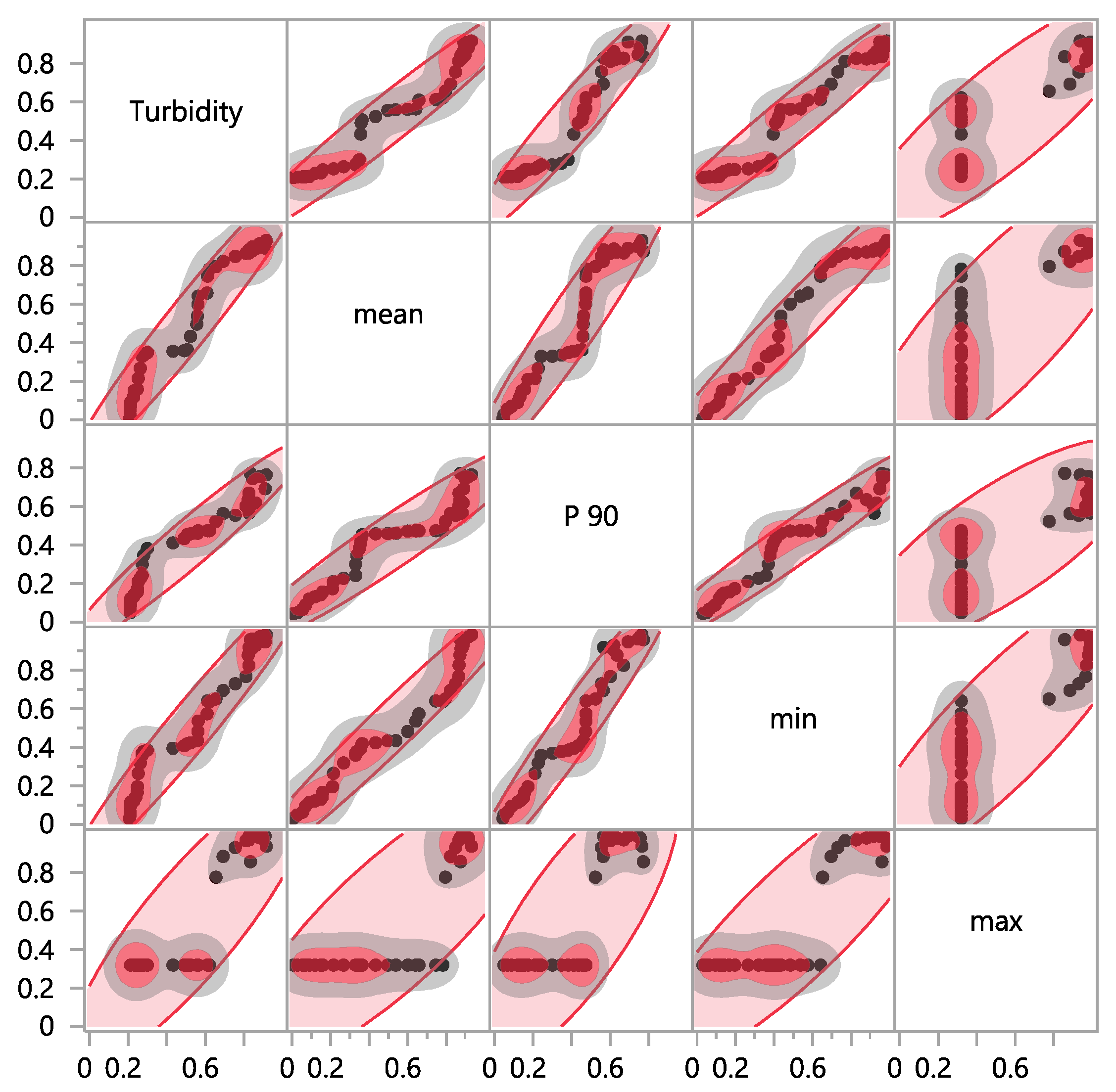
Multi variance analysis shows a strong correlation between the mean in situ readings and the mean image values of estimated MCI, GNDVI, and NDTI (Figure 5, Figure 6 and Figure 7). Table 2 expresses the correlation coefficient of the water quality parameters under investigation.
The minimum and maximum pixel did not show a strong association with in situ measurements. The reason behind this weak relationship is that both minimum and maximum pixel values were considered as the analysis range anomalies [29].
There was no significant difference between the in-situ surface water sampling across different climatic conditions and the subsurface measurements taken by the dam authority, which might be understood as reaching the saturation level of the investigated water quality parameters [30]. Therefore, this leads to water being classified as of a low quality that cannot be safely or directly used [31].
The temporal analysis of the estimated remotely sensed indices ensured regression stability [7] based on robust linear coherence between the actual and estimated water quality parameters examined in the current research study.
While Van Wagtendonk et al. [32] failed to establish a strong association using Landsat data, red-edge bands of Sentinel-2 proved to be efficiently reliable for estimating water quality parameters specified in inland water [33].
According to Gitelson et al. [34], Odermatt et al. [35], and Vesali et al. [36] estimation of chlorophyll concentration underwater turbidity conditions was satisfactorily conducted using several models based on accurate spectral measurements. However, developing complex models seems to be difficult, due to the broad bandwidth of Operational Land Imager (OLI) data. This requires the development of a different method that is applicable to OLI data.
Nevertheless, complex models for chlorophyll estimations based on Landsat OLI data are hard to develop because of Landsat OLI broad bandwidth in the near-infrared and thermal infrared regions [37]. Previously, scholarly work of Walthall et al. [38] and Adam et al. [39] reported weaknesses in the association of middle infrared and chlorophyll concentrations in water using Landsat ETM+ data. This was explained by the penetration limitations of Landsat ETM+ bands in deep water [40,41].
Estimation of N concentration in agricultural crops and its spatial distribution has been the goal of several scholarly works because of its importance to soil fertilization [42,43]. However, estimation of dissolved N is confined to a limited number of earth observation sensors equipped specifically with the red-edge region of the spectrum [44].
Regression analysis between the actual N concentration and the estimated index was exercised on four different zonal statistic types. The mean and the P 90 values were more coherent than the actual data with a correlation coefficient of 0.9699 and 0.9596, respectively, while maximum and minimum values were less representative of the actual N concentration. The increase in the dissolved N in the dam lake is a sign of pollution pressure to the water quality on the catchment scale [45,46]. However, the N concentration is monitored by the local authority at the outflow, disregarding only the separation distribution of the pollutant which can be assessed using remote sensing data [47,48].
Water turbidity as a sign of sedimentation processes was initially considered by Carpenter [49] utilizing Landsat Thematic Mapper data. The algorithm was consequently developed to consider the change in the central bandwidth of the recent sensors as Doxaran [50] reported using Satellite Probatoire de l’Observation de la Terre (SPOT) images. The duality of the bands at 645 and 850 nm of suspended particulate matter proved to be effective in turbidity detection, especially in inland water [51]. Similarly, Sentinel-2 central band wavelengths in the near-infrared region cover the designated bands for suspended particulate detection, making the sensor capable of estimation of water turbidity in a precise manner [52,53].
4. Conclusions
The routine monitoring of water quality parameters is costly and requires constant laboratory supplies and efforts. The implemented methodologies, as well as the comprehensive assessments, answered the questions concerning the feasibility of using a linear empirical approach to estimate the designated water quality parameters across temporal remote sensing data. Estimation of chlorophyll, nitrogen content, and water turbidity were successfully achieved utilizing remote sensing data acquired from Sentinel-2. Red-edge bands of Sentinel-2 are the keystone feature of the sensor for estimating the addressed water quality parameters in a reliable manner. Moreover, the mean values of the raster data showed a high correlation with the actual data from the conducted laboratory examinations. Therefore, a consistent empirical model could be determined.
Author Contributions
Conceptualization, M.E. and I.G.; Methodology, M.E. and A.O.; Validation, J.B., P.G. and M.E.; Formal Analysis, M.E. and A.O.; Writing—Original Draft Preparation, M.E.; Writing—Review & Editing, M.E. and A.O.
Acknowledgments
This project was funded by the Deanship of Scientific Research (DSR) at King Abdulaziz University, Jeddah, under grant no. KEP-MSc-01-155-38. The authors, therefore, acknowledge with thanks DSR for technical and financial support.
Conflicts of Interest
The authors declare no conflict of interest.
References
- Elhag, M.; Bahrawi, J.A. Conservational use of remote sensing techniques for a novel rainwater harvesting in arid environment. Environ. Earth Sci. 2014, 72, 4995–5005. [Google Scholar] [CrossRef]
- Elfeki, A.; Al-Shabani, A.; Bahrawi, J.; Alzahrani, S. Quick urban flood risk assessment in arid environment using HECRAS and dam break theory: Case study of Daghbag Dam in Jeddah, Saudi Arabia. In Euro-Mediterranean Conference for Environmental Integration, 1917–19; Springer: Berlin, Germany, 2017. [Google Scholar]
- Elhag, M.; Bahrawi, J.A. Spatial assessment of landfill sites based on remote sensing and GIS techniques in Tagarades, Greece. Desalin. Water Treat. 2017, 91, 395–401. [Google Scholar] [CrossRef]
- Clevers, J.G.P.W.; Gitelson, A.A. Remote estimation of crop and grass chlorophyll and nitrogen content using red-edge bands on Sentinel-2 and -3. Int. J. Appl. Earth Observ. Geoinf. 2013, 23, 344–351. [Google Scholar] [CrossRef]
- Mei, H.; Xiong, Y.; Xie, S.; Guo, S.; Li, Y.; Guo, B.; Zhang, J. The impact of long-term school-based physical activity interventions on body mass index of primary school children–a meta-analysis of randomized controlled trials. BMC Public Health 2016, 16, 205. [Google Scholar] [CrossRef] [PubMed]
- Morris, C.E.; Monier, J.E. The ecological significance of biofilm formation by plant-associated bacteria. Annu. Rev. Phytopathol. 2003, 41, 429–453. [Google Scholar] [CrossRef] [PubMed]
- Psilovikos, A.; Elhag, M. Forecasting of remotely sensed daily evapotranspiration data over Nile Delta region, Egypt. Water Resour. Manag. 2013, 27, 4115–4130. [Google Scholar] [CrossRef]
- Mojaddadi, H.; Pradhan, B.; Nampak, H.; Ahmad, N.; Ghazali, A.H.b. Ensemble machine-learning-based geospatial approach for flood risk assessment using multi-sensor remote-sensing data and GIS. Geomat. Nat. Hazards Risk 2017, 8, 1080–1102. [Google Scholar] [CrossRef]
- Elhag, M.; Bahrawi, J.A. Soil salinity mapping and hydrological drought indices assessment in arid environments based on remote sensing techniques. Geosci. Instrum. Methods Data Syst. 2017, 6, 149–158. [Google Scholar] [CrossRef] [Green Version]
- Chen, J.; Zhu, W.; Tian, Y.Q.; Yu, Q.; Zheng, Y.; Huang, L. Remote estimation of colored dissolved organic matter and chlorophyll-a in Lake Huron using Sentinel-2 measurements. J. Appl. Remote Sens. 2017, 11, 036007. [Google Scholar] [CrossRef]
- Liu, H.; Li, Q.; Shi, T.; Hu, S.; Wu, G.; Zhou, Q. Application of Sentinel 2 MSI images to retrieve suspended particulate matter concentrations in Poyang Lake. Remote Sens. 2017, 9, 761. [Google Scholar] [CrossRef]
- Raghunathan, T.E.; Lepkowski, J.M.; van Hoewyk, J.; Solenberger, P. A multivariate technique for multiply imputing missing values using a sequence of regression models. Survey Methodol. 2001, 27, 85–96. [Google Scholar]
- Kalagi, S.S.; Mali, S.S.; Dalavi, D.S.; Inamdar, A.I.; Im, H.; Patil, P.S. Limitations of dual and complementary inorganic–organic electrochromic device for smart window application and its colorimetric analysis. Synth. Metals 2011, 161, 1105–1112. [Google Scholar] [CrossRef]
- Merino, L.; Edberg, U.; Fuchs, G.; Åman, P. Liquid chromatographic determination of residual nitrite/nitrate in foods: NMKL collaborative study. J. AOAC Int. 2000, 83, 365–375. [Google Scholar]
- Ellis, J.; Cummings, V.; Hewitt, J.; Thrush, S.; Norkko, A. Determining effects of suspended sediment on condition of a suspension feeding bivalve (Atrina zelandica): Results of a survey, a laboratory experiment and a field transplant experiment. J. Exp. Mar. Biol. Ecol. 2002, 267, 147–174. [Google Scholar] [CrossRef]
- Kutser, T. Quantitative detection of chlorophyll in cyanobacterial blooms by satellite remote sensing. Limnol. Oceanogr. 2004, 49, 2179–2189. [Google Scholar] [CrossRef] [Green Version]
- Alikas, K.; Kangro, K.; Reinart, A. Detecting cyanobacterial blooms in large North European lakes using the Maximum Chlorophyll Index. Oceanologia 2010, 52, 237–257. [Google Scholar] [CrossRef] [Green Version]
- Matthews, M.W.; Bernard, S.; Robertson, L. An algorithm for detecting trophic status (chlorophyll-a), cyanobacterial-dominance, surface scums and floating vegetation in inland and coastal waters. Remote Sens. Environ. 2012, 124, 637–652. [Google Scholar] [CrossRef]
- Salem, S.I.; Higa, H.; Kim, H.; Kazuhiro, K.; Kobayashi, H.; Oki, K.; Oki, T. Multi-algorithm indices and look-up table for chlorophyll-a retrieval in highly turbid water bodies using multispectral data. Remote Sens. 2017, 9, 556. [Google Scholar] [CrossRef]
- Gitelson, A.; Merzlyak, M.N. Quantitative estimation of chlorophyll-a using reflectance spectra: Experiments with autumn chestnut and maple leaves. J. Photochem. Photobiol. B: Biol. 1994, 22, 247–252. [Google Scholar] [CrossRef]
- Gitelson, A.A.; Merzlyak, M.N. Remote estimation of chlorophyll content in higher plant leaves. Int. J. Remote Sens. 1997, 18, 2691–2697. [Google Scholar] [CrossRef]
- Hunt, E.R.; Hively, W.D.; McCarty, G.W.; Daughtry, C.S.T.; Forrestal, P.J.; Kratochvil, R.J.; Carr, J.L.; Allen, N.F.; Fox-Rabinovitz, J.R.; Miller, C.D. NIR-green-blue high-resolution digital images for assessment of winter cover crop biomass. GISci. Remote Sens. 2011, 48, 86–98. [Google Scholar] [CrossRef]
- Lacaux, J.P.; Tourre, Y.M.; Vignolles, C.; Ndione, J.A.; Lafaye, M. Classification of ponds from high-spatial resolution remote sensing: Application to Rift Valley Fever epidemics in Senegal. Remote Sens. Environ. 2007, 106, 66–74. [Google Scholar] [CrossRef]
- Johnson, N.L.; Kotz, S.; Balakrishnan, N. Continuous Univariate Distributions, 2nd ed.; wiley series in probability and mathematical statistics: Applied probability and statistics; Wiley: New York, NY, USA, 1995; vol. 2. [Google Scholar]
- Dutilleul, P.; Stockwell, J.D.; Frigon, D.; Legendre, P. The Mantel test versus Pearson’s correlation analysis: Assessment of the differences for biological and environmental studies. J. Agric. Biol. Environ. Stat. 2000, 131–150. [Google Scholar] [CrossRef]
- Nevitt, J.; Hancock, G.R. Improving the root mean square error of approximation for nonnormal conditions in structural equation modeling. J. Exp. Educ. 2000, 68, 251–268. [Google Scholar] [CrossRef]
- Psilovikos, A.; Margoni, S.; Psilovikos, A. Simulation and trend analysis of the water quality monitoring daily data in Nestos river delta. Contribution to the sustainable management and results for the years 2000–2002. Environ. Monit. Assess. 2006, 116, 543–562. [Google Scholar] [CrossRef] [PubMed]
- Elhag, M.; Bahrawi, J.A. Realization of daily evapotranspiration in arid ecosystems based on remote sensing techniques. Geoscientific Instrumentation. Meth. Data Syst. 2017, 6, 141. [Google Scholar]
- Howe, C.Q.; Purves, D. Range image statistics can explain the anomalous perception of length. Proc. Natl. Acad. Sci. 2002, 99, 13184–13188. [Google Scholar] [CrossRef] [PubMed] [Green Version]
- Debels, P.; Figueroa, R.; Urrutia, R.; Barra, R.; Niell, X. Evaluation of water quality in the Chillán River (Central Chile) using physicochemical parameters and a modified water quality index. Environ. Monit. Assess. 2005, 110, 301–322. [Google Scholar] [CrossRef]
- Chapman, D.V. Water Quality Assessments: A Guide to the Use of Biota, Sediments and Water in Environmental Monitoring; CRC Press: New York, NY, USA, 2002. [Google Scholar]
- Van Wagtendonk, J.W.; Root, R.R.; Key, C.H. Comparison of AVIRIS and Landsat ETM+ detection capabilities for burn severity. Remote Sens. Environ. 2004, 92, 397–408. [Google Scholar] [CrossRef]
- Delegido, J.; Verrelst, J.; Alonso, L.; Moreno, J. Evaluation of Sentinel-2 red-edge bands for empirical estimation of green LAI and chlorophyll content. Sensors 2011, 11, 7063–7081. [Google Scholar] [CrossRef]
- Gitelson, A.A.; Gurlin, D.; Moses, W.J.; Barrow, T. A bio-optical algorithm for the remote estimation of the chlorophyll-a concentration in case 2 waters. Environ. Res. Lett. 2009, 4, 045003. [Google Scholar] [CrossRef]
- Odermatt, D.; Gitelson, A.; Brando, V.E.; Schaepman, M. Review of constituent retrieval in optically deep and complex waters from satellite imagery. Remote Sens. Environ. 2012, 118, 116–126. [Google Scholar] [CrossRef] [Green Version]
- Vesali, F.; Omid, M.; Kaleita, A.; Mobli, H. Development of an android app to estimate chlorophyll content of corn leaves based on contact imaging. Comput. Electron. Agric. 2015, 116, 211–220. [Google Scholar] [CrossRef]
- Barsi, J.A.; Schott, J.R.; Hook, S.J.; Raqueno, N.G.; Markham, B.L.; Radocinski, R.G. Landsat-8 thermal infrared sensor (TIRS) vicarious radiometric calibration. Remote Sens. 2014, 6, 11607–11626. [Google Scholar] [CrossRef]
- Walthall, C.; Dulaney, W.; Anderson, M.; Norman, J.; Fang, H.; Liang, S. A comparison of empirical and neural network approaches for estimating corn and soybean leaf area index from Landsat ETM+ imagery. Remote Sens. Environ. 2004, 92, 465–474. [Google Scholar] [CrossRef]
- Adam, E.; Mutanga, O.; Rugege, D. Multispectral and hyperspectral remote sensing for identification and mapping of wetland vegetation: A review. Wetl. Ecol. Manag. 2010, 18, 281–296. [Google Scholar] [CrossRef]
- Gianinetto, M.; Villa, P.; Lechi, G. Postflood damage evaluation using Landsat TM and ETM+ data integrated with DEM. IEEE Trans. Geosci. Remote Sens. 2006, 44, 236–243. [Google Scholar] [CrossRef]
- Elhag, M.; Psilovikos, A.; Sakellariou-Makrantonaki, M. Land use changes and its impacts on water resources in Nile Delta region using remote sensing techniques. Environ. Dev. Sustainability 2013, 15, 1189–1204. [Google Scholar] [CrossRef] [Green Version]
- Boegh, E.; Soegaard, H.; Broge, N.; Hasager, C.B.; Jensen, N.O.; Schelde, K.; Thomsen, A. Airborne multispectral data for quantifying leaf area index, nitrogen concentration, and photosynthetic efficiency in agriculture. Remote Sens. Environ. 2002, 81, 179–193. [Google Scholar] [CrossRef]
- Chen, P.; Haboudane, D.; Tremblay, N.; Wang, J.; Vigneault, P.; Li, B. New spectral indicator assessing the efficiency of crop nitrogen treatment in corn and wheat. Remote Sens. Environ. 2010, 114, 1987–1997. [Google Scholar] [CrossRef] [Green Version]
- Elhag, M. Evaluation of different soil salinity mapping using remote sensing techniques in arid ecosystems, Saudi Arabia. J. Sens. 2016. [Google Scholar] [CrossRef]
- Margoni, S.; Psilovikos, A. Sustainable management of Agiasma Lagoon–River Nestos delta—Using RE MO. S. daily monitoring data of water quality and quantity parameters: Trends, assessments, and natural hazards for the years 2000–2002. Desalination 2010, 250, 287–296. [Google Scholar] [CrossRef]
- Elhag, M.; Bahrawi, J.A.; Galal, H.K.; Aldhebiani, A.; . Al-Ghamdi, A.A. Stream network pollution by olive oil wastewater risk assessment in Crete, Greece. Environ. Earth Sci. 2017, 76, 278. [Google Scholar] [CrossRef]
- He, B.; Oki, K.; Wang, Y.; Oki, T.; Yamashiki, Y.; Takara, K.; Miura, S.; Imai, A.; Komatsu, K.; Kawasaki, N. Estimation of monthly potential nitrogen load from agricultural and forest watersheds using quickbird remote sensing imagery. Int. Arch. Photogramm. Remote Sens. Spat. Inf. Sci. 2010, 38, 528–533. [Google Scholar]
- Cilia, C.; Panigada, C.; Rossini, M.; Meroni, M.; Busetto, L.; Amaducci, S.; Boschetti, M.; Picchi, V.; Colombo, R. Nitrogen status assessment for variable rate fertilization in maize through hyperspectral imagery. Remote Sens. 2014, 6, 6549–6565. [Google Scholar] [CrossRef]
- Carpenter, D.; Carpenter, S. Modeling inland water quality using Landsat data. Remote Sens. Environ. 1983, 13, 345–352. [Google Scholar] [CrossRef]
- Doxaran, D.; . Froidefond, J.-M.; Lavender, S.; Castaing, P. Spectral signature of highly turbid waters: Application with SPOT data to quantify suspended particulate matter concentrations. Remote Sens. Environ. 2002, 81, 149–161. [Google Scholar] [CrossRef]
- Dogliotti, A.I.; Ruddick, K.G.; Nechad, B.; Doxaran, D.; Knaeps, E. A single algorithm to retrieve turbidity from remotely-sensed data in all coastal and estuarine waters. Remote Sens. Environ. 2015, 156, 157–168. [Google Scholar] [CrossRef] [Green Version]
- Toming, K.; Kutser, T.; Laas, A.; Sepp, M.; Paavel, B.; Nõges, T. First experiences in mapping lake water quality parameters with Sentinel-2 MSI imagery. Remote Sens. 2016, 8, 640. [Google Scholar] [CrossRef]
- Gernez, P.; Lafon, V.; Lerouxel, A.; Curti, C.; Lubac, B.; Cerisier, S.; Barillé, L. Toward Sentinel-2 High Resolution Remote Sensing of Suspended Particulate Matter in Very Turbid Waters: SPOT4 (Take5) Experiment in the Loire and Gironde Estuaries. Remote Sens. 2015, 7, 9507–9528. [Google Scholar] [CrossRef] [Green Version]
Figure 1.
Location of the study area.

Figure 2.
Maximum chlorophyll index (MCI) regression analysis with respect to different zonal statistics values.
Figure 2.
Maximum chlorophyll index (MCI) regression analysis with respect to different zonal statistics values.


Figure 3.
Green normalized difference vegetation index (GNDVI) regression analysis with respect to different zonal statistics values.
Figure 3.
Green normalized difference vegetation index (GNDVI) regression analysis with respect to different zonal statistics values.

Figure 4.
Normalized difference turbidity index (NDTI) regression analysis with respect to different zonal statistics values.
Figure 4.
Normalized difference turbidity index (NDTI) regression analysis with respect to different zonal statistics values.

Figure 5.
Scatter plot matrix of MCI—actual and different zonal estimated values.

Figure 6.
Scatter plot matrix of GNDVI—actual and different zonal estimated values.

Figure 7.
Scatter plot matrix of NDTI—actual and different zonal estimated values.


Table 1.
Summary of fit analysis.
| Header | MCI | |||
|---|---|---|---|---|
| Mean | P 90 | Min | Max | |
| RSquare | 0.966900 | 0.886912 | 0.930364 | 0.947727 |
| RSquare Adj | 0.966051 | 0.884012 | 0.928579 | 0.946386 |
| Root Mean Square Error | 0.039628 | 0.073256 | 0.075427 | 0.051299 |
| Mean of Response | 0.452561 | 0.465951 | 0.489893 | 0.447380 |
| GNDVI | ||||
| RSquare | 0.940660 | 0.920928 | 0.917046 | 0.096571 |
| RSquare Adj | 0.939138 | 0.918900 | 0.914919 | 0.073406 |
| Root Mean Square Error | 0.068546 | 0.076428 | 0.090124 | 0.014555 |
| Mean of Response | 0.492012 | 0.520620 | 0.510049 | 0.420685 |
| NDTI | ||||
| RSquare | 0.941958 | 0.921015 | 0.942222 | 0.736541 |
| RSquare Adj | 0.940470 | 0.918990 | 0.940741 | 0.729786 |
| Root Mean Square Error | 0.077774 | 0.062725 | 0.075304 | 0.156997 |
| Mean of Response | 0.513581 | 0.413256 | 0.504930 | 0.532880 |
Table 2.
The correlation coefficient of the water quality parameters.
| Header | Color | Mean | P 90 | Min | Max |
|---|---|---|---|---|---|
| Color | 1.0000 | 0.9833 | 0.9418 | 0.9646 | 0.9735 |
| Mean | 1.0000 | 0.9648 | 0.9748 | 0.9607 | |
| P 90 | 1.0000 | 0.9786 | 0.8863 | ||
| Min | 1.0000 | 0.9271 | |||
| Max | 1.0000 | ||||
| Nitrate | Mean | P 90 | Min | Max | |
| Nitrate | 1.0000 | 0.9699 | 0.9596 | 0.9576 | 0.3108 |
| Mean | 1.0000 | 0.9859 | 0.9874 | 0.3553 | |
| P 90 | 1.0000 | 0.9951 | 0.4076 | ||
| Min | 1.0000 | 0.4040 | |||
| Max | 1.0000 | ||||
| Turbidity | Mean | P 90 | Min | Max | |
| Turbidity | 1.0000 | 0.9707 | 0.9597 | 0.9705 | 0.8582 |
| Mean | 1.0000 | 0.9559 | 0.9771 | 0.8206 | |
| P 90 | 1.0000 | 0.9676 | 0.7770 | ||
| Min | 1.0000 | 0.8616 | |||
| Max | 1.0000 |
© 2019 by the authors. Licensee MDPI, Basel, Switzerland. This article is an open access article distributed under the terms and conditions of the Creative Commons Attribution (CC BY) license (http://creativecommons.org/licenses/by/4.0/).
Share and Cite
MDPI and ACS Style
Elhag, M.; Gitas, I.; Othman, A.; Bahrawi, J.; Gikas, P. Assessment of Water Quality Parameters Using Temporal Remote Sensing Spectral Reflectance in Arid Environments, Saudi Arabia. Water 2019, 11, 556. https://doi.org/10.3390/w11030556
AMA Style
Elhag M, Gitas I, Othman A, Bahrawi J, Gikas P. Assessment of Water Quality Parameters Using Temporal Remote Sensing Spectral Reflectance in Arid Environments, Saudi Arabia. Water. 2019; 11(3):556. https://doi.org/10.3390/w11030556
Chicago/Turabian StyleElhag, Mohamed, Ioannis Gitas, Anas Othman, Jarbou Bahrawi, and Petros Gikas. 2019. "Assessment of Water Quality Parameters Using Temporal Remote Sensing Spectral Reflectance in Arid Environments, Saudi Arabia" Water 11, no. 3: 556. https://doi.org/10.3390/w11030556
Note that from the first issue of 2016, this journal uses article numbers instead of page numbers. See further details here.