Advanced Numerical Modeling of Sediment Transport in Gravel-Bed Rivers


1
Institute of Hydraulic and Water Resources Engineering, Technische Universität München, Arcisstrasse 21, D-80333 München, Germany
2
Faculty of Mechanical Engineering, Thuyloi University, 175 Tay Son, Dong Da, Hanoi 100000, Vietnam
*
Author to whom correspondence should be addressed.
Water 2019, 11(3), 550; https://doi.org/10.3390/w11030550
Submission received: 15 February 2019
/
Revised: 11 March 2019
/
Accepted: 13 March 2019
/
Published: 17 March 2019
(This article belongs to the Section Hydraulics and Hydrodynamics)
Abstract
:Understanding the alterations of gravel bed structures, sediment transport, and the effects on aquatic habitat play an essential role in eco-hydraulic and sediment transport management. In recent years, the evaluation of changes of void in bed materials has attracted more concern. However, analyzing the morphological changes and grain size distribution that are associated with the porosity variations in gravel-bed rivers are still challenging. This study develops a new model using a multi-layer’s concept to simulate morphological changes and grain size distribution, taking into account the porosity variabilities in a gravel-bed river based on the mass conservation for each size fraction and the exchange of fine sediments between the surface and subsurface layers. The Discrete Element Method (DEM) is applied to model infiltration processes and to confirm the effects of the relative size of fine sediment to gravel on the infiltration depth. Further, the exchange rate and the bed porosity are estimated while using empirical formulae. The new model was tested on three straight channels. Analyzing the calculated results and comparing with the observed data show that the new model can successfully simulate sediment transport, grain sorting processes, and bed change in gravel-bed rivers.
1. Introduction
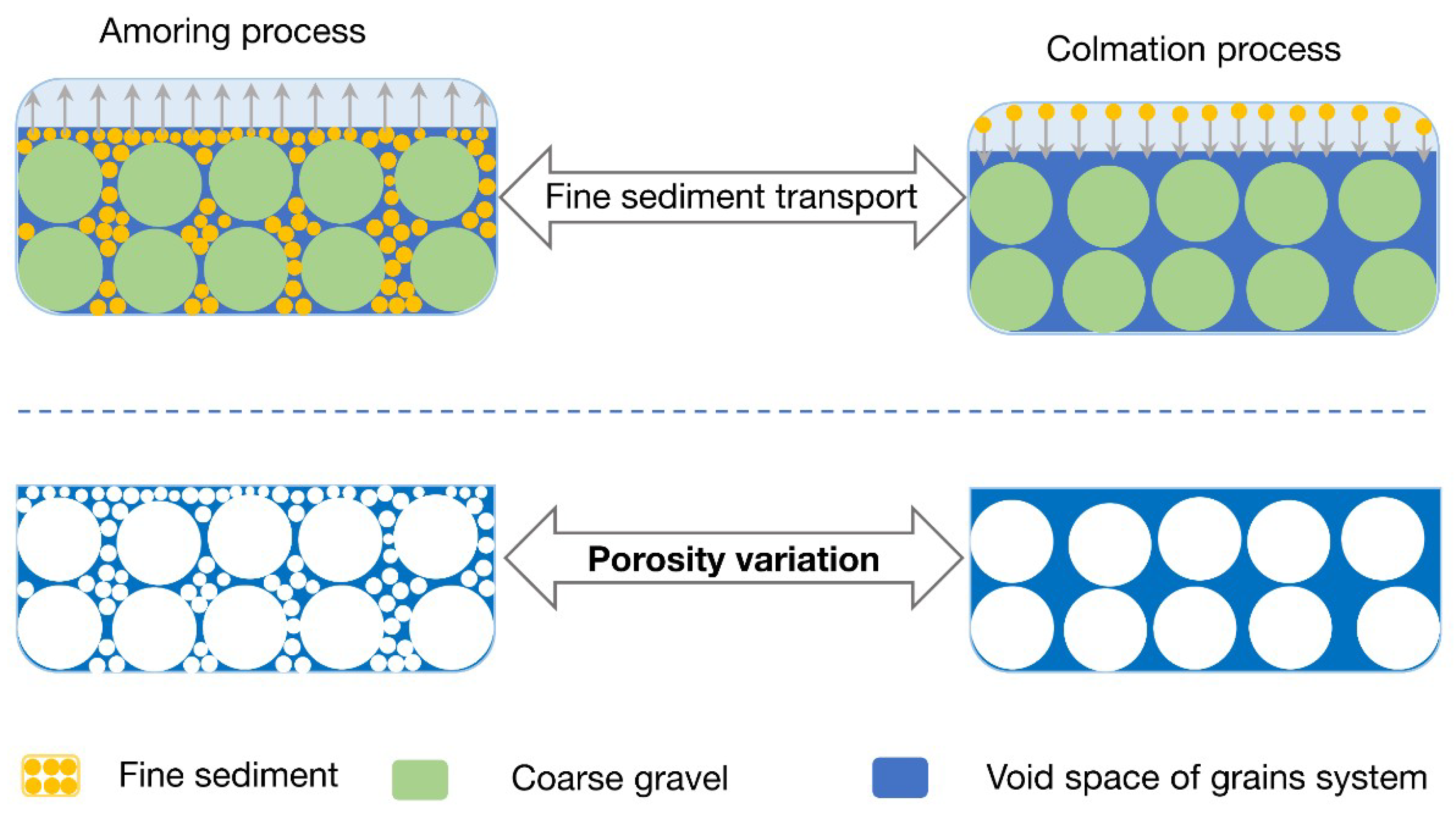
Sediment transport processes that are due to flowing water in gravel-bed rivers can be formed from bed load, suspended load, and movement inside the bed layer. More importantly, in the same hydraulics condition, the transport rate of coarse size fraction may be different from the rate of fine size fraction. These reasons lead to the distinct forms of gravel-bed rivers. Due to high-flow velocity, all of the finer particles may be eroded, leaving a layer of coarse particles. When the flow is unable to carry the coarse particles, then no more erosion occurs, which is known as an armoring process [1,2]. Inversely, under low-flow conditions, sediment transport can cause the extensive infiltration of fine sediment into void spaces in coarse bed material [3,4], which is also known as clogging or colmation [5,6] (see Figure 1).
The change in grain size distribution of coarse and fine sediment not only leads to the variation in bed profile, but it also mainly results in the change in bed porosity defined as a fraction of the volume of voids over the total volume of the gravel-bed river. According to [7,8], the porosity of sand-gravel mixtures can vary from about 0.10 to 0.50. For example, the measured porosity values in the Rhine River range from 0.06 to 0.48 [9].
The study of variation in porosity is vital for fluvial geomorphology assessment as well as in river ecosystem management. From a river management point of view, the amount of fine sediment stored in the void space of gravel-bed up to 22% [10] may be neglected during calculation by considering constant porosity. Furthermore, the porosity may exert strong influence on the rate of bed level changes [11,12]. The impact of void space of gravel-bed on habitats for fish and aquatic insects is essential, and particularly the importance of assessing the change in the void structure of the bed material has been pointed out strongly [13].
To model sediment transport processes as well as bed deformation, multi-layer models were applied for graded sediment transport. Despite the considerable variations of porosity, most of the conventional models assumed that the porosity of bed material is constant. Therefore, sediment transport in the form of infiltration into the void spaces of the coarse bed, or fine particles in sublayers and the entrainment of fine sediment into flow from the substrates, is not taken into account. This assumption can be inappropriate for simulating the sediment transport and bed variation in gravel-bed rivers. Toro-Escobar et al. [14] accounted for this process in terms of an appropriate transfer or exchange function at the interface between the surface layer and substrate. Based on the data from a large-scale experiment on the aggradation and the selective deposition of gravel, they proposed an empirical form for the transfer function, where material that is transferred to the substrate can be represented as a weighted average of bedload and surface material, with a bias toward bedload. Applying this function with the assumption of a constant porosity, Cui [15] developed a numerical model for sand entrainment/infiltration from/into the subsurface. The model was applied to study the dynamics of grain size distributions, including the fractions of sand in sediment deposits and on the channel bed surface. Further, Sulaiman et al. [16] proposed an approximated bed variation model while considering the change in bed porosity, where the thickness of each layer is assumed to be constant and equal. Furthermore, the exchange between bed material and the transported sediment only takes place on the surface layer, and sediment transport from an upper layer to the lower layer is neglected. These assumptions are improper in gravel-bed rivers, where finer sediment possibly drops into the subsurface layer.
To bridge above knowledge gap, in this paper we develop a numerical hydromorphological model that considers the bed porosity change and the exchange flux of fine sediment between two different bed layers. Further, the Discrete Element Method (DEM) is employed for modeling the infiltration processes. We test the new numerical model for three straight gravel-bed open channels. The calculated results are then compared with the observed data to verify the improved model.
2. Methodology
As usual, the structure of our proposed model consists of two modules: (1)—hydrodynamic module; and, (2)—sediment transport and bed variation module. In the hydrodynamic module, the backwater equation is employed for low Froude number conditions and the quasi normal flow assumption is applied for the high Froude number flow conditions. The friction slope is calculated with the Keulegan formulation, which is used for calculating the transport rate in the sediment transport and bed variation module. More details regarding the water flow equations can be found in the studies that were conducted by Cui and Parker [15,17,18,19,20]. The flow module interacts with sediment transport and bed variation module that is based on the mechanism of quasi-steady morphodynamic time-stepping, in which the interaction between the flow and bed profile is considered in two different times. More specifically, at each time step of the flow calculation, the bed level is considered to be constant, and the sediment transport is assumed not to effect the flow, whereas in the process of bed calculation, the flow is assumed to be invariant. Subsequently, the water depth, velocity, as well as the bed roughness are adjusted based on the results of the sediment transport and bed variation module. The calibrated roughness is used in the hydraulic module in the next time step. Since previous models contained some limitations, we developed a new sediment transport and bed variation module, which is presented in detail in the following sections.
In principle, the bed topography in a channel is related to the transport of both bed load and suspended load. In the case of a coarse-material bed, the influence of suspended load is negligible, whereas the bed load is predominant. Further, suspended sediment load is the fine material that moves through the channel in the water column. These materials are kept in suspension by the upward flux of turbulence that is generated at the bed of the channel. The upward currents must equal or exceed the particle fall-velocity for suspended sediment load to be sustained. In this paper, we assume the turbulent flow to be small, therefore we only consider bed load in sediment transport modelling.
The governing equations for flow, sediment transport, and bed variation are numerically solved while applying the finite volume method with the required initial and boundary conditions.
2.1. Sediment Transport and Bed Variation Module
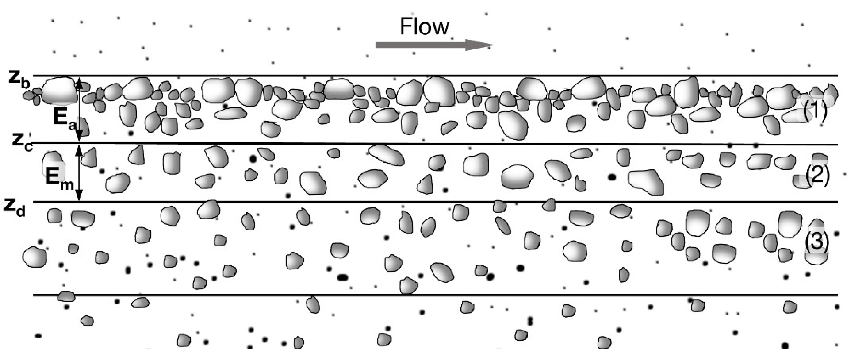
The size-fraction method is applied to divide bed material into some size-fractions. Each fraction is characterized by an average grain size and volume percentage of occurrence in the bed material and presented these components as the probability of different group. Applying the so-called multi-layer concept, we divide the vertical bed structure into different layers. Figure 2 shows a diagram of this structure consisting of one active layer and several substrate layers. Sediment particles are continuously exchanged between the flow and the active layer. Generally, the sediments in this layer can be transported as bed load, suspended load, or infiltration. Furthermore, they can move between the active layer and sublayers, depending mostly on the bed porosity and grain size distribution, as it will be discussed below in Section 2.3. For example, sediments are exchanged between the active layer and substrates when the bed scours or fills, as well as when filtration occurs. As erosion occurs, the entrainment of sediment particles from the active layer and its ensuing downward displacement causes particles from substrate layers to be mixed with those in the active layer. On the contrary, the deposition of sediment particles on the bed leads to an upward displacement of the active layer and the initiation of new substrate layers. At high flow discharges, fine sediments in the top substrate (2) may also be attracted to the surface layer and entrained flow.
Furthermore, the riverbed morphology in nature can be related to all three types of sediment transport that are mentioned above (bed load, suspended load, and infiltration of fine sediment). As mentioned above, when turbulent flow is week or the settling velocity of sediment particle is more significant than critical shear stress velocity, sediment particle only moves in the forms of bed load or infiltration. For the sake of simplicity of this paper, we assume that
- The horizontal surface is unchanged zd = 0, so sediment sorting occurs only in the active layer (1) and the upmost sublayer (2); i.e., the bed consists of only two layers.
- The bed sediment is moving under two forms: infiltration or bed load.
- The flow and sediment transport are one-dimensional.
The change in the bed elevation is calculated using the law of continuity of bed sediment in the active layer:
Where x = The coordinate axis along the flow direction; z = The coordinate axis along the vertical direction; t = time; p = p(x,z,t) = bed porosity; qb = qb(x,t) = total specific volumetric bed load discharge. Its fraction qb,j is determined by experiment or semi-experiment when considering non-equilibrium bed load [21]. In this study, the fractional bed load rate is calculated while using the bed-load equation proposed by Wilcock and Crowe [22]. Further, Equation (1) can also be rewritten as:
Applying the theorem of mean values and Leibniz integral rule for two finite integrals in the left-hand side of Equation (2) yields:
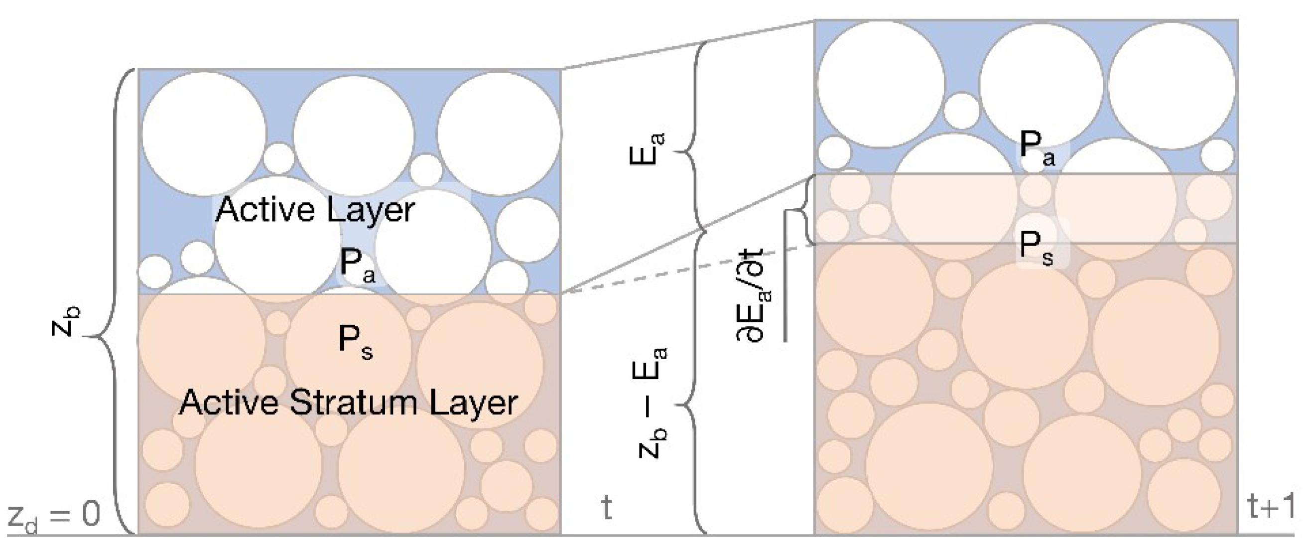
In which pa = pa(x,t) = the average porosity of active layer; ps = ps(x,t) = the average porosity of sublayer layer (Figure 3). If the porosity of layers is constant, the porosity source term Sp = 0 and Equation (3) becomes the Exner equation. Therefore, Equation (3) can be considered as the expansion of the Exner equation, when considering the variation of porosity in space and time.
Assuming that the grain sorting in an active layer only occurs under the flow interaction and exchange process between the active layer and the active stratum layer and while applying the mass conservation law in the active layer, we obtain the equation for the change of size fraction, as below:
Equation (4) can be rewritten in the following form:
which βa,j = the size fraction of active layer; and, βb,j = the size fraction j of sediment transport in the form of bed load. The function SF,j expresses the exchange process of the active layer and sublayers of the size fraction j. Determining the SF,j value can be considered as the quantification of the bottom infiltration process and Section 2.2 provides a detailed description of this function.
Based on the mass conservation and assuming that the grain sorting of the active stratum layer is caused by the exchange process between the surface layer and subsurface one, we get the following equation for the size fraction change in the subsurface layer:
In which βs,j is the size fraction j of sediment in the subsurface layer. As can be seen in Equations (3)–(6), the bed porosity variation and the sediment exchange between two neighbor bed layers are considered. Furthermore, the experimental studies show that the bed porosity depends on two main parameters: grain size distribution and compaction degree of bed material. Section 2.3 describes details regarding the determination of porosity.
2.2. Infiltration Process
The infiltration process is the movement of fine sediment, such as sand and silt, into void space in gravel-bed due to gravity. The infiltration process will stop when the sizes of these voids are small enough. Typically, bed sediments are divided into two different sizes: Fine sediment includes particles with a size less than 2 mm and coarse sediment with a particle size larger than 2 mm. The relative mean size of coarse sediment Dm and fine sediment dm can be used to evaluate the depth of the infiltration process. For example, according to [23], if the ratio (Dm/dm) of river bed less than 10, then fine sediment is almost impossible to infill through the void space of the gravel bed. If this ratio is between 10 and 30, then fine sediments will be deposited in the void space of the top gravel-bed layer and create a sand seal. If 30 < Dm/dm < 70, some fine sediments will be clogged at the void of the upper layer, but they will not clearly create a sand seal. When the ratio Dm/dm greater than 70, all of the fine sediment will settle down to the bottom of the gravel bed. These critical values may be changed when the bed material consists of almost uniform spherical particles for fine and coarse sediments. In other words, the infiltration process depends on the characteristic parameters of the bottom (including the size distribution as well as the shape of the sediment particles). Additionally, this process depends on the near bottom hydraulic conditions, i.e., near-bed flow water and flow through the void space of the gravel bed. Cui et al. [3] proposed a theoretical model, in which the fraction of fine sediment decreases exponentially along with the depth of the gravel bed. Wooster et al. [24] and Gibson et al. [25] also used this hypothesis with laboratory observation data to develop their models, in which the fine reduction sediment is determined as a function of gravel depth.
Based on the empirical equation of Toro-Escobar et al. [14], the following equation can be proposed to quantify the exchange between the active layer and active stratum layer for the fine fraction of size class j [26]:
where coefficient c can be considered as a parameter of the model. As can be seen in Equation (7), the function SF,j depends on sediment discharge of size class j, the time variation of bed porosity and active layer thickness. However, effects of sediments in the stratum layer was not yet considered in this equation.
Cundall and Strack initially proposed the Discrete Element Method (DEM) [27] to model the mechanical behavior of granular flows and to simulate the forces acting on each particle and its motion. Typically, a particle can be classified into two types of motion in DEM: translation and rotation. The momentum and energy of particles are exchanged during collisions with their neighbors or a boundary wall (contact forces), and particle-fluid interactions, as well as gravity. While applying Newton’s second law of motion, we can determine the trajectory of each i-particle (including its acceleration, velocity, and position) from the following equations:
where mi = the mass of a particle i; = the velocity of a particle; = gravity acceleration; = interaction force between particle i and particle k (contact force); = interaction force between the particle i and the fluid; I = moment of inertia; = angular velocity; di = diameter of the grain i; = directional contact = vector connecting the center of grains i and k.
We use a contact force model that is based on the principle of spring-dashpot, as well as the suggestions of Hertz–Mindlin [28]. The contact force is obtained from the force analysis method; the stiffness and damping factors are analyzed in two directions: orthogonal and tangent of the contact surface between the two grains:
(n) and (τ) are known as two components of contact force in a normal direction and tangential direction; ki = stiffness of grain i; δi,k = The characteristic of the contact and displacement (also called the length of the springs in the two directions above); αi = damping coefficient; and, Δui = relative velocity of grain at the moment of collision. Additionally, following Coulomb, the product of the coefficient of friction μ and the orthogonal force component determines the value of tangential friction. In the nonlinear contact force, the Hertz–Mindlin model, which is the tangential force component, will increase until the ratio (f(τ)/f(n)) reaching a value of μ, and it keeps the maximum value until the particles are no longer in contact with each other. A detail of the force models, as well as the method for determining the relevant coefficients, can be found in [28].
After calculating all of the forces acting on the sediment particles, as well as the velocity and the position of the particle at a previous time step, we can determine the velocity and position of grain at present step based on solving Equations (8) and (9). The grain size distribution, as well as the bed porosity for whole the domain, can be defined afterwards. As a result, we can also estimate the exchange rate of the fine fraction between different bed layers.
2.3. Porosity Estimation
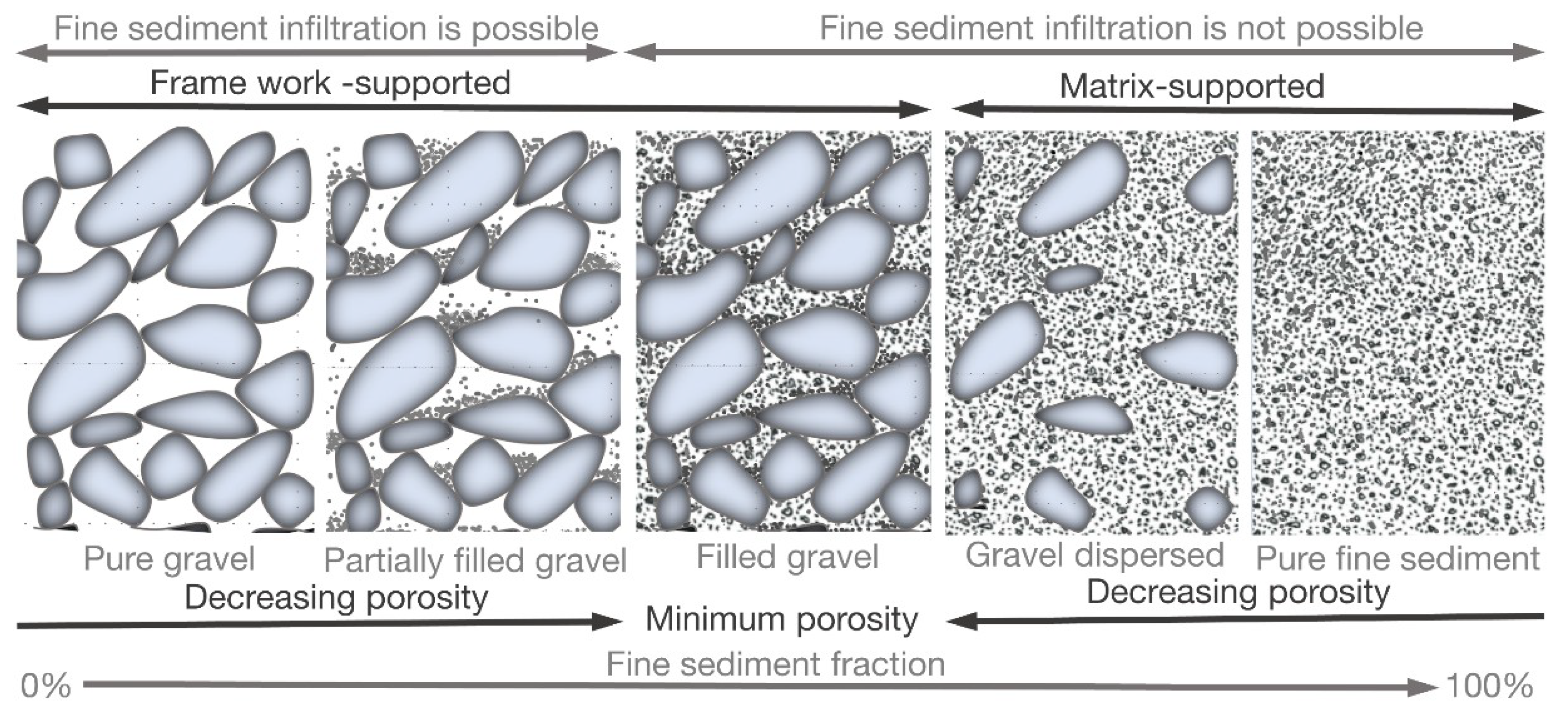
Figure 4 shows a qualitative dependency between the bed porosity and fine size fraction, as well as their influence on the infiltration process (based on Church [29]). Additionally, the porosity of the gravel-bed is smallest when it is filled by fine sediment.
Similarly to Bui et al. [30], we consider the volume of a unit bed sediment with a porosity p consisting of two types of sediment: coarse and fine, then the absolute volume (without porosity) of the bed sediment is (1 − p). We assume that the ratio of fine particle size to coarse sediment is smaller than 0.154 (called as critical ratio) and fine particles do not affect the arrangement of coarse particles during the infiltration process.
Further, if the bed does not contain fine sediments, then the total volume of coarse sediment is (1 − p(D)), where p(D) is porosity of coarse sediment. Correspondingly, the relative ratio of coarse sediment volume to the total volume of bed sediment is determined as:
While applying the same definition and similar symbols p(d) and f(d) for fine sediment, we have f(d) = (1 − f(D)) and obtained the correlation between porosity of bed and porosity of coarse sediment and the relative proportions of fine sediment, as follows:
The minimum of bed porosity is (p(D) × p(d)). Substituting this value into Equation (13), we obtain the relationship between the bottom porosity and the characteristics of fine sediment for this case, as follows:
Following Nunez-Gonzalez et al. [31], Equation (14) can be applied to calculate the porosity of the bed, with a predominance of the sand matrix (e.g., see right panel of Figure 4). Since Equations (13) and (14) have been obtained for the ideal gravel beds, their modifications that are based on measured data can be more suitable for different bed conditions. For example, Koltermann and Gorelick [32] proposed the following expression for calculating the bed porosity:
The bed porosity reaches the minimum value pmin when the fraction of fine sediment is approximately equal to the porosity of the coarse sediment. Kamann et al. [33] has improved Equation (15) and then proposed the same expression to calculate the bed porosity:
where f(d)min is a fine size fraction when the bed porosity reaches the minimum value.
Yu and Standish [34,35] developed a semi-analytical model for different grain sizes, which can be one of the best models in predicting the porosity of sand gravel mixtures [9]. The model is based on the assumptions that the grains are spherical sharp, no deformable, and uniform density, and random packing. Although these assumptions are not always valid for natural sediments, the model can be applied for natural sediments with angular grains [34].
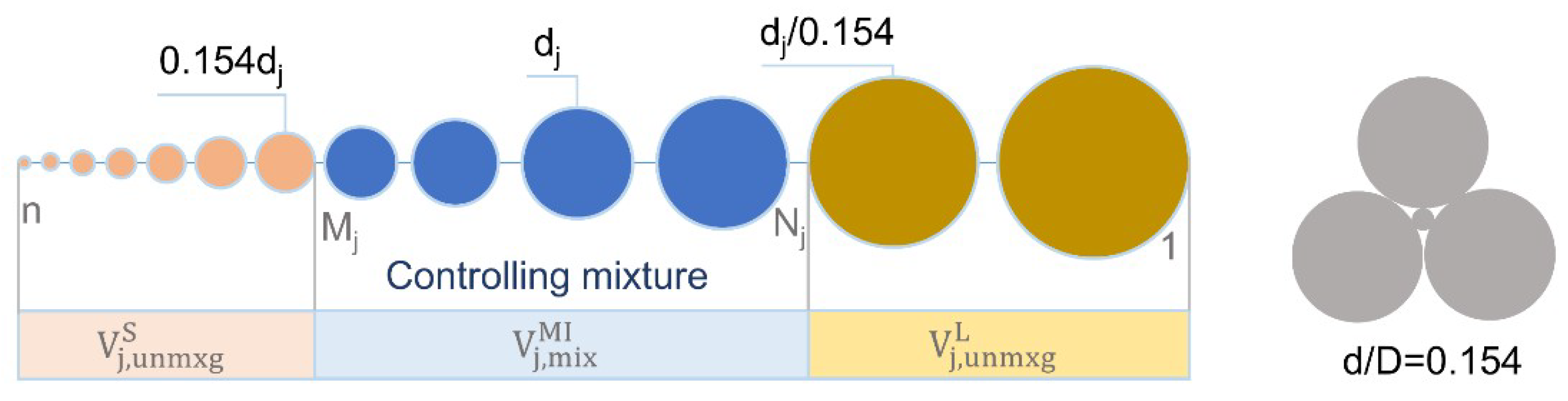
We consider the mixture of n component with diameter d1 > d2 > ... > dj > … > dn, initial specific volume V1, V2, …, Vj, …, Vn, and size fraction β1, β2, …, βj, …, βn.
For each component j, the parameters Mj and Nj are calculated using the critical size ratio (d/D = 0.154) and comparing with the other diameters.
The grain mixture is divided into partial specific volumes for each (dj) grain based on Mj, Nj (see Figure 5). The middle zone is the controlling mixture of grain size jth (occupation), the first zone, and the last zone is presented filling mechanism. Particles in the first zone can fill in the structure component with diameter jth without disturbing in structure, and diameter jth is also filled in last zone structure.
where: is the specific volume of component jth with porosity pj, which consists of three parts (Figure 5).
presents the occupation mechanism (unmixing effect): change the skeleton of the controlling component. Because the partial specific of controlling mixture is the same as the specific volume when only these controlling components themselves form a packing mixture.
where is the initial specific volume; are the empirical coefficients, which express the joint action of the mixture. present the filling mechanism (Mixing effect). The semi empirical interaction functions f(j,i) and g(j,i) depend on the diameter and density of controlling mixture, which Yu and Standish modified [34]. The equations are slightly different from that by the previous equations. This is particularly true for spherical particles where the initial porosity is relatively low.
The overall specific volume of mixture (V) is obtained by the optimization and porosity of mixture (p) gained by simple equation
3. Results and Discussions
3.1. Infiltration of Fine Sediments into Gravel-Bed
The infiltration processes of fine sediment into gravel-bed are numerically tested with different sizes of particles. The tests are based on Gibson’s experiment [25]. Numerical simulations are carried out for a flume with a width of 0.15 m and a length of 0.5 m. The flume is filled with a granular bed of spherical gravels having different diameters with the same specific weight (2700 kg/m3). We refer to fine sediment as sand. The simulations are carried out for a bed with uniform sand and gravel (Case 1) and a graded sand-gravel-bed (Case 2). The sediment bed layer is 0.1 m thick with the following characteristics (Table 1):
- Case-1: uniform gravel size D = 10 mm and uniform sand with a size d defined from the following size ratios:Critical ratio for tetrahedral packing d/D = 0.154;One and halftime of the critical ratio for tetrahedral packing d/D = 0.231; and,Critical ratio for cubical packing d/D = 0.414.
- Case-2: Multi size fractions of sand and gravel bed:Sand with a mean diameter of dm = 0.26 mm and standard deviation of σ(d) = 1.94; and,Gravel with a mean diameter of Dm = 7.1 mm and a standard deviation of σ(D) = 1.35.
Case 2 is similar to the experiment No.2 conducted by Gibson [25] with very slow water flow. Hence, the effects of water flow on infiltration and packing processes can be neglected in the numerical model.
A DEM model is implemented to test the influence of the size ratio of the fine to coarse sediment on the vertical distribution of the bed materials. We develop the DEM model that is based on the open source package LIGGGHTS [36]. In the model, we neglect the interaction between the flows and the particles, because of low flow velocity. For that, non-slip boundary flow condition is applied for the simulations. The force acting on the particle consists of the gravity, Archimedes, and contact forces.
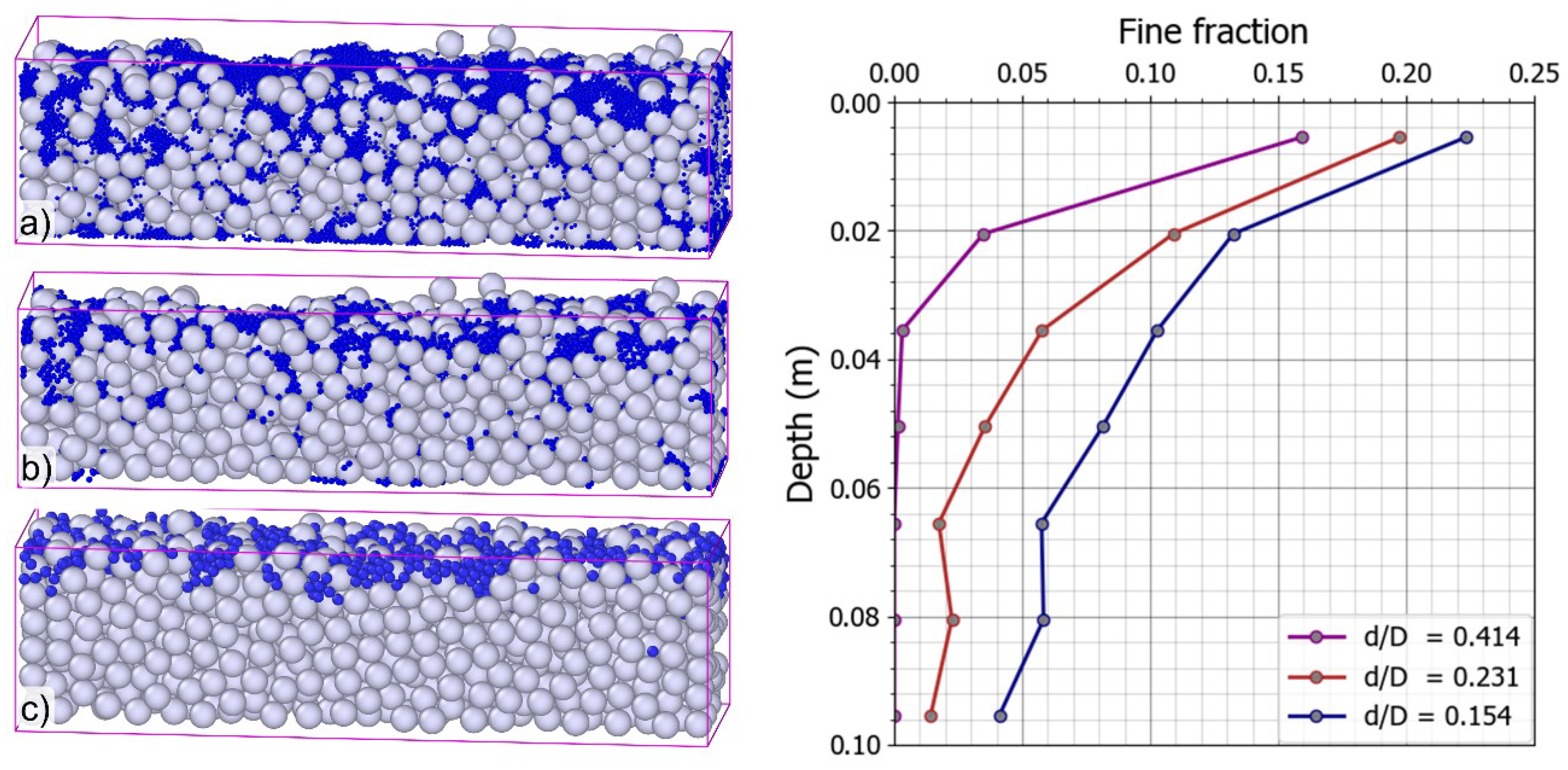
In Case 1, during the first 20,000 time steps, the gravel-bed was generated by random packing with porosity p(D) = 0.454. The fine sediment was fed over the bed surface from the 20,000th step. The simulation process was stopped when the void space in the bed surface has been clogged or the bed has been fulfilled with fine sediments. Figure 6 presents the structure of the gravel-bed, as well as the vertical distribution of fine sediments with three different sizes at the end of simulation time. The simulated results are qualitatively comparable to the experimental results that were conducted by [37,38] for the idealized packing of the purely bimodal bed sediments. For the case d/D = 0.154 (Figure 6a), it can be observed that the fine sediments mostly filled into the void space and were then trapped there. However, while increasing the size ratio to d/D = 0.231, the fine sediment infiltrated into only a part of the void space (Figure 6b). Figure 6c shows the results for the case d/D = 0.414, where the initial void space was smaller than the diameters of fine sediment. The fine sediment was trapped in the bed surface and could not move down into the gravel bed. As expected, the calculated results confirm that the size ratio has a significant effect on the infiltration process, as well as the vertical distribution of the fine sediments.
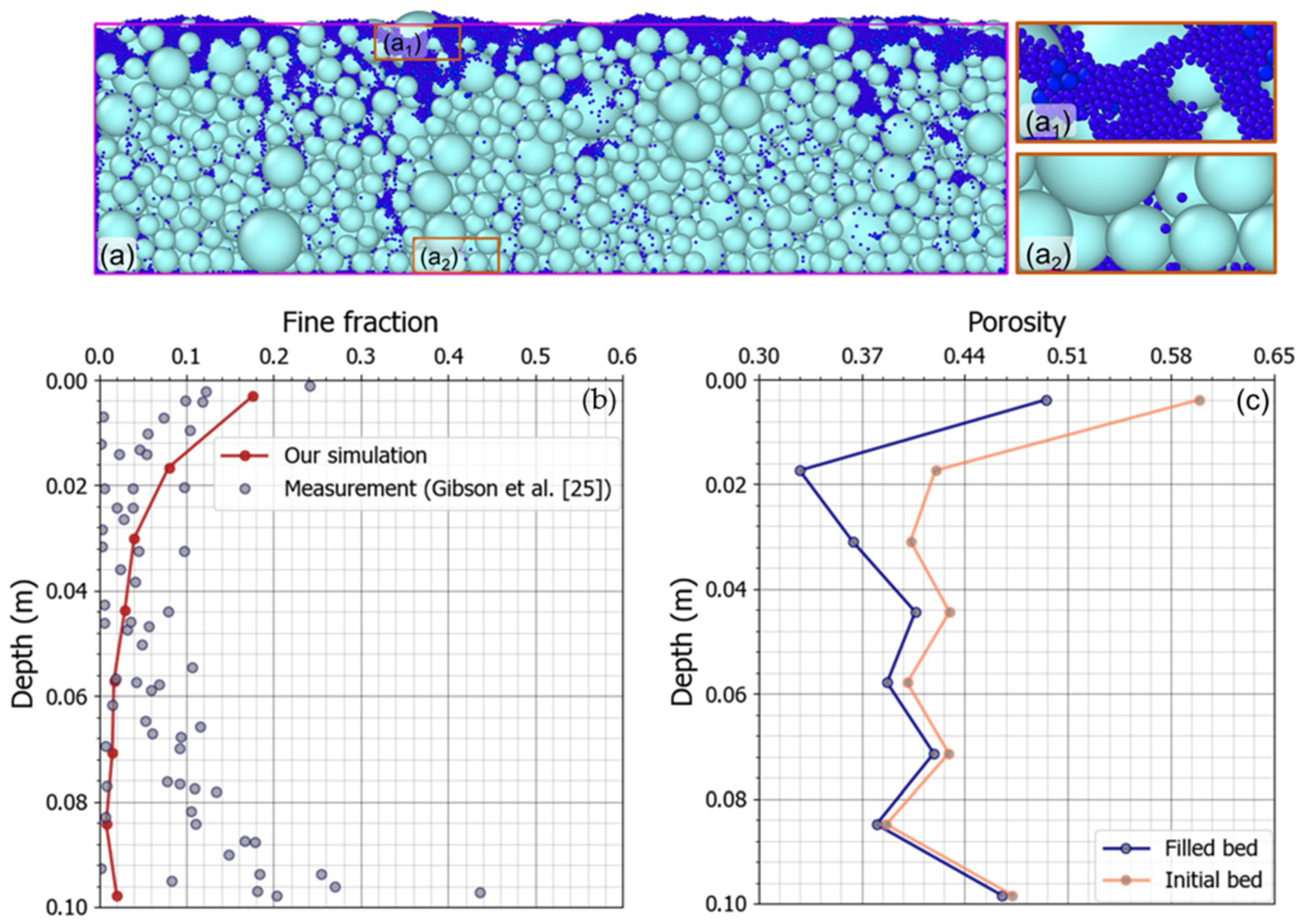
Further simulations were carried out for Case 2, with a median grain size of the non-uniform fine sediments dm = 0.26 mm and standard deviation σ(d) = 1.94. The gravel mixture has a median grain size of Dm = 7.1 mm and the end of simulation time σ(D) =1.35. Random packing during the first 41,000 time steps with porosity p(D) = 0.407 generated the gravel-bed. The infiltration process was stopped when the top gravel layer has been filled. Figure 7a shows the bed materials along the flume centerline at the end of the simulation, where the gradation of saturated gravels with percolated fines can be seen. Furthermore, as the pores on the surface layer were filled with fine sediment, fine particles could not infiltrate through this layer and saturate the subsurface pore space. Figure 7b compares the mean values of the simulated fine fractions along the depth, with the observations that were conducted by Gibson et al. [25].
In the model, we used about 1150 coarse sediment particles for Case 1 and 3550 for Case 2. Depending on the grain size, three values of the number of the fine sediment particles (770, 6000, and 36,740) were implemented for Case 1. For Case 2, we used 113,770 fine particles. The computational time that is required for Case 2 is about 4 h on a PC −3.9 GHz. The computational effort of study on large scale could be enormous and only completed successfully with extensive use of computer.
It needs to be emphasized that Gibson et al. [25] conducted the experiments in a large flume with a very low water velocity (no bed sediment transport), while due to high computational requirements, our DEM model only considered a small window (0.15 m wide and 0.5 m long) with quiescent water. It could be a reason of the differences between our results and measured data. However, it can be said that we obtained a qualitative good agreement with the experimental results. Figure 7c shows a variation of the calculated porosity along the depth at the beginning and the end of simulation time, which is correlated to the grain-size distribution.
3.2. Bed Form Movement and Porosity Variation
The simulation was conducted in a 500 m long straight channel with a rectangular cross section, a uniform specific water discharge of 23 m3/s/m, a constant water elevation of 10 m long the channel, and the initial bed level defined, as follows:
The bed mixture was sorted into two fractions (d1 = 1 mm; d2 = 7 mm), which was then used to compose a desired size gradation. The initial size fractions are (βa,1 = 0.75 and βa,2 = 0.25) in the active layer and (βS,1 = 0.65 and βS,2 = 0.35) in the stratum layer.
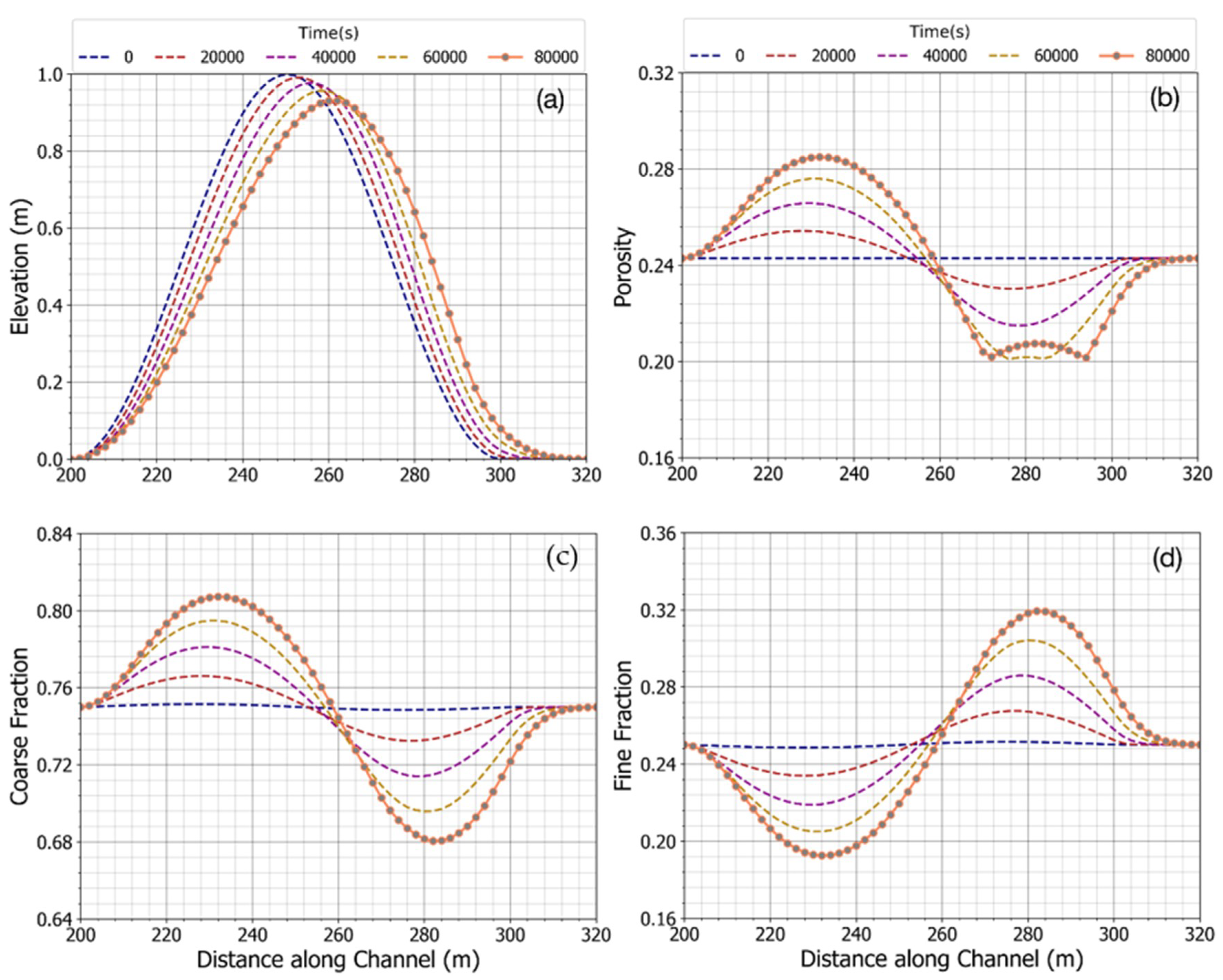
Figure 8 presents changes in bed characteristics over time. Figure 8a shows the bed elevation at different time steps, the dune moved forward with the water flow, and reduced its height. Especially, in the front of the dune, the gradient of sediment discharge is positive due to the increase in flow velocity, and this caused bed erosion. Inversely, sediment is deposited on the back of the dune, where the gradient of sediment discharge is negative. Figure 8c,d depict the size fraction of coarse and fine sediments along the channel. Since the fine sediment on the left side of the dune was eroded, transported by the increased water velocity, and deposited on the right side of dune due to the reduced water velocity. It led to an increasing in the coarse fraction on the left side of the dune and decreasing of the coarse fraction on the right side. An opposite picture was obtained for distibution of the fine fraction. Variation of the size fractions resulted in changing the bed porosity (Figure 8b). Porosity gets a minimal value of 0.2 on the right side of the dune at time 80,000 (s), where the coarse fraction is approximately 0.69 and the fine fraction about 0.31. Increasing the fine fraction from this value the bed porosity becomes larger. For the left side of the dune (coarse fraction > 0.73), growing the coarse fraction increases the bed porosity.
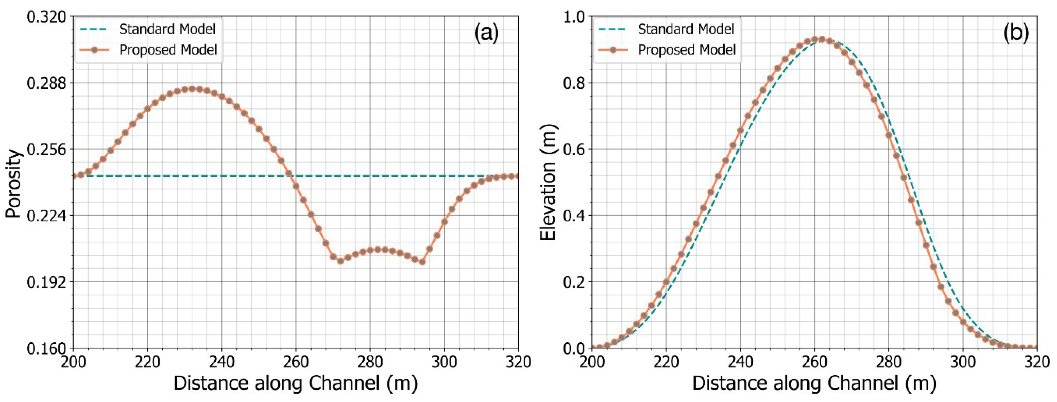
Figure 9 compares the new model with a conventional model (with a constant porosity). In the conventional model, a constant value of 0.25 for bed porosity was selected, while in the new model, it varied in a range from 0.21 to 0.28 due to size fraction change at the end of the calculation time. It can be seen that, due to the larger values of the calculated bed porosity on the left side of the dune, the predicted bed elevations were slightly higher than those that were obtained from the conventional model. An opposite picture can be seen on the right side of the dune. The new model provided a qualitatively good picture about the bed form movement and porosity variation in the channel.
3.3. Sulaiman’s Experiment
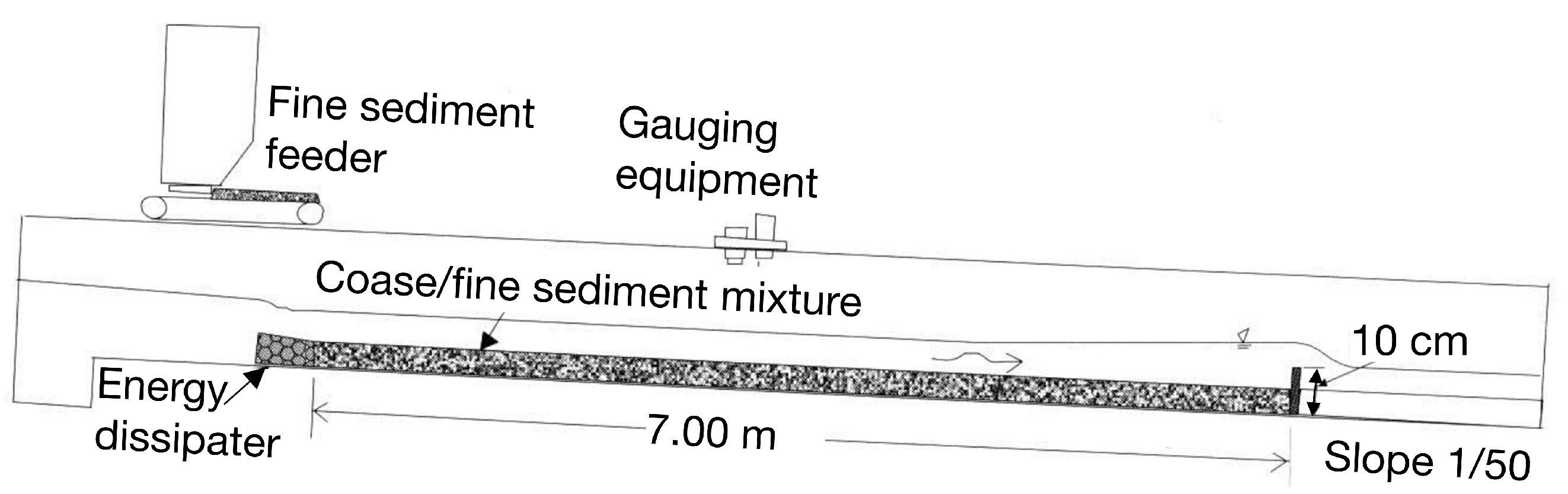
To identify the transformation processes of void structure in gravel bed, Sulaiman et al. [16] conducted experiments in a flume with a width of 0.40 m, a depth of 0.40 m, and a working length of 7.0 m (Figure 10). The slope of the flume was adjusted to 1/50. Water discharge was kept nearly constant for all of the runs and circulated. A sediment mixture was initially placed in the working section and then scraped flat. The thickness of the sediment layer was 5.3 cm. A weir with a height of 10 cm was placed at the end of the working section. The bed consisted of a coarse and fine fraction of sediments. The coarse fraction ranges from 4.75 mm to 26.5 mm in size with d50 = 15 mm, and the fine fraction ranges from 0.5 mm to 4.75 mm with d0 = 2 mm. The sediments were mixed and then thoroughly homogenized. Experiments have been carried out for two situations. In Run-1, no sediment was supplied at the inlet; coarse sediment did not move actively, and only fine sediment was removed from the bed. In Run-2, an amount of the fine sediment fraction was continuously fed from the upstream of the flume, and these fine sediments could be deposited into the coarse bed or transported downstream. The condition of the riverbed at the end of Run-1 was used as an initial condition of Run-2. Cumulative time steps for Run-1 are 20, 65, 130, and 250 min and for Run-2 were 30, 50, 66, and 82 min. The total duration of Run-1 and Run-2 was 332 min. Table 2 summarizes the experimental conditions. Water depth h and velocity v are the initial average water depth and velocity in the uniform region. More details of the experiments description can be seen in [16].
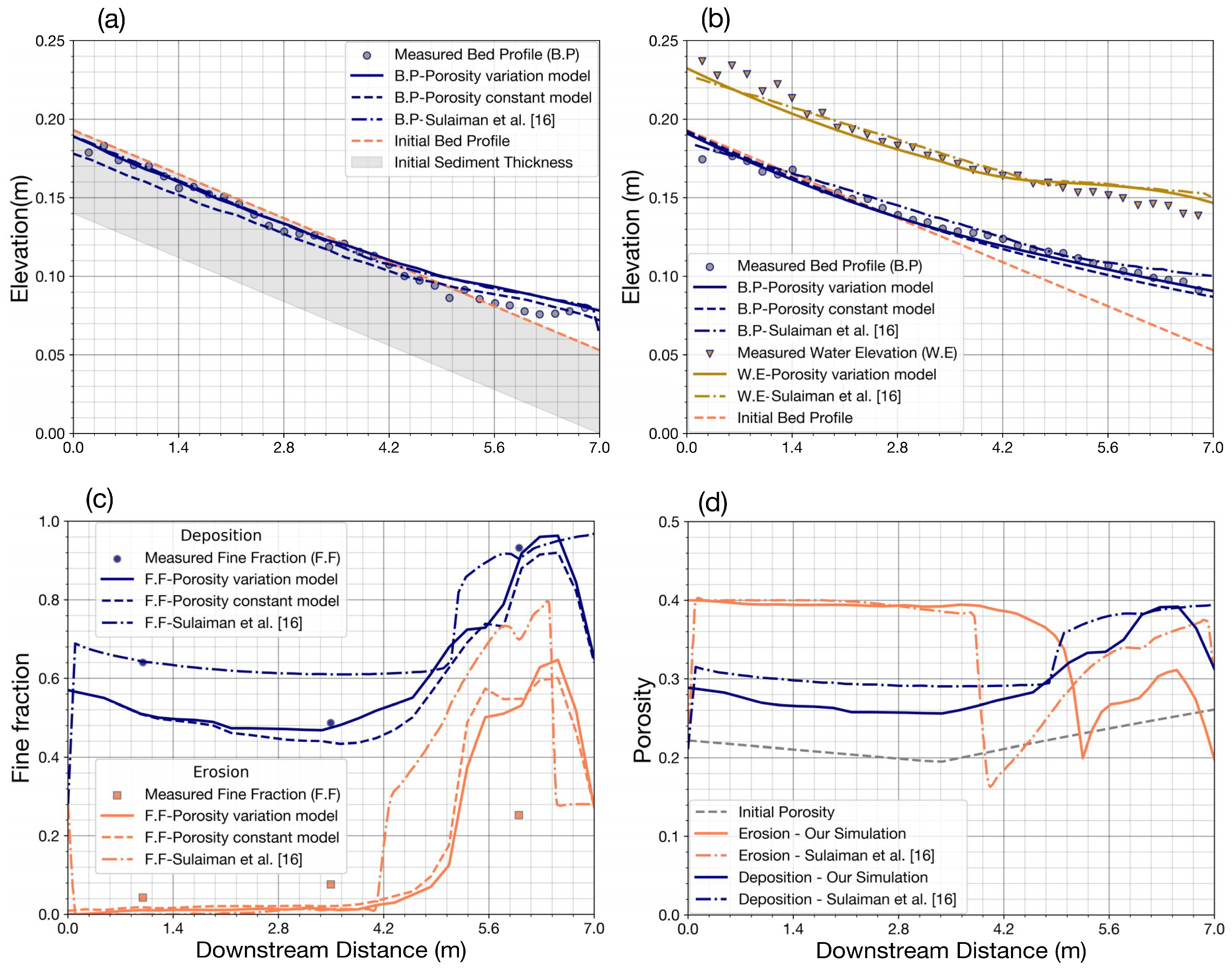
Figure 11 shows the comparison of our results and Sulaiman’s results for the erosion case (Run-1) and deposition case (Run-2) with regard to bed elevation, fine fraction, and porosity between, respectively. In Figure 11a, the results of our bed elevation with porosity variation are better than those in the constant models, because of the incorporation of porosity changes in our model. The erosion of the upstream part in our model is a good fit with the experimental result, while larger erosion of the upstream part of the constant model can be seen. The stored fine sediment in the pores of gravel-bed leaved the coarse layer increased the void space, but they did not contribute to lowering of the bed level. This result is consistent with the findings of [10]. Moreover, the storage capacity of the gravel-bed reached 30%, while fine sediment fraction was greater than the range of 31–37%. As a result, the bed elevation at the final step is lower than the initial elevation because of the erosion of fine sediment on the surface. Downstream, due to the bed load formula, the bed profile of our and Sulaiman’s simulation are not good, which has not been developed for a mixture of two particle groups with very different grain sizes [39].
Figure 11b present bed elevation, fine fraction, and porosity to compare our results and Sulaiman’s results for the deposition case (Run 2). The results of our bed elevation fit well when compared to the results that were derived from Sulaiman and constant models. However, the bed level differences in all models are small due to a hidden function in the bed load equation for fine sediment on the upper gravel-bed surface, and because bed shear stress is larger than the critical shear stress of most fine sediment. More detail about the comparison between the models can be seen in Table 3.
Grain size distribution (size fractions) due to sediment exchange in the bed surface layer was investigated for two cases, one for erosion and other for deposition. The calculated results were compared with the Sulaiman’s and constant porosity models, as well as the observed data.
Figure 11c shows the fine fraction along the flume in these two cases. In the erosion case, fine sediment is removed from the bed material on the upstream part and it is deposited on the downstream part. The fine sediment fraction upstream is nearly zero and equal to 0.6 downstream (Figure 11c—coral color line). In the deposition case (navy color line), the supplied fine sediment completely filled the pore of the bed material increasing fine fraction to 0.6 upstream and 0.96 downstream. The results show that our model with variable porosity is slightly better than the constant porosity model, because the fine fraction in our model tends to fluctuate widely when compared with those in the constant model. The results can be partly explained by considering the fine sediment that is stored in void spaces exchanged with sediment transport may lead to porosity changes. In Figure 11c—fine fraction for the deposition case—the results of Sulaiman are better than our results (navy color line), inversely our model performs better in the erosion case (coral color line). The slight difference in the fine fraction results between our porosity variation model and the Sulaiman porosity variation model and the minor variation in comparison with the porosity variation model and the constant model can also be seen in Table 3.
Figure 11d depicts the porosity due to sediment exchange on the surface layer in the cases of sediment erosion (coral color lines) and deposition (navy color lines). At the initial condition, the fine fraction upstream and downstream is from 37% to 22%, respectively, and the diameter ratio is dcoarse/dfine = 7.5, the minimum porosity is equal to 0.195. At the end of the simulation, the fine sediment wholly filled in the void structure of gravel in the middle of the flume. In the erosion case, most of the fine particles are removed from gravel upstream (x = 4.2 m) and the porosity is reached the maximum value of 0.4. Afterward, the porosity decreased to a minimum value of 0.195 when the fine fraction increased from 0.22 to 0.30. In the deposition case, in contrast to the erosion case, the fine fraction is greater than 0.30, and the porosity is proportional to a fine fraction. The increase in porosity in the deposition case is less than that in the erosion case.
3.4. SAFL’s Experiment
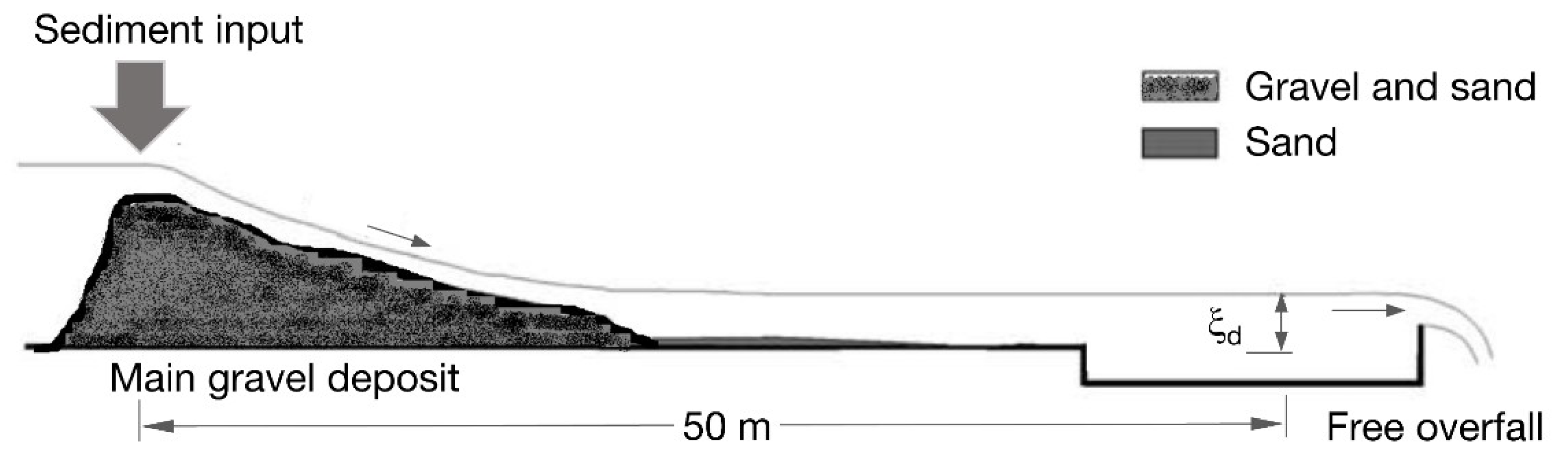
The SAFL (St. Anthony Falls Laboratory) downstream fining experiment is known as the most comprehensive set of experiments to date on gravel transport that have been performed at the St. Anthony Falls Laboratory in Minnesota by Parker and his co-workers [40,41,42]. The experiment was conducted in a 0.305-m wide and 50-m long flume with an initial concrete-bottom slope of 0.002 (Figure 12), a constant water discharge, and a constant sediment feed rate. The flume is ponded at its downstream reach by setting a constant water surface elevation at the downstream end, which drives channel aggradation and downstream fining. The relevant parameters for the run are given in Table 4. Seal et al. provide a full description of the experimental data [43].
We simulated bed elevation, grain size distribution, and porosity in the surface layer and subsurface layer while considering the sediment exchange between these layers. A bed load equation that was developed by Wilcock & Crowe [22] was used to calculate sediment discharge for each size fraction. The thickness of the active layer is changing over time and space based on the multiplication of D90 and the coefficient of active layer thickness nactive = 2. The roughness height also varies over time and space, as defined by the product of D90 and roughness coefficient of nk = 1.8.
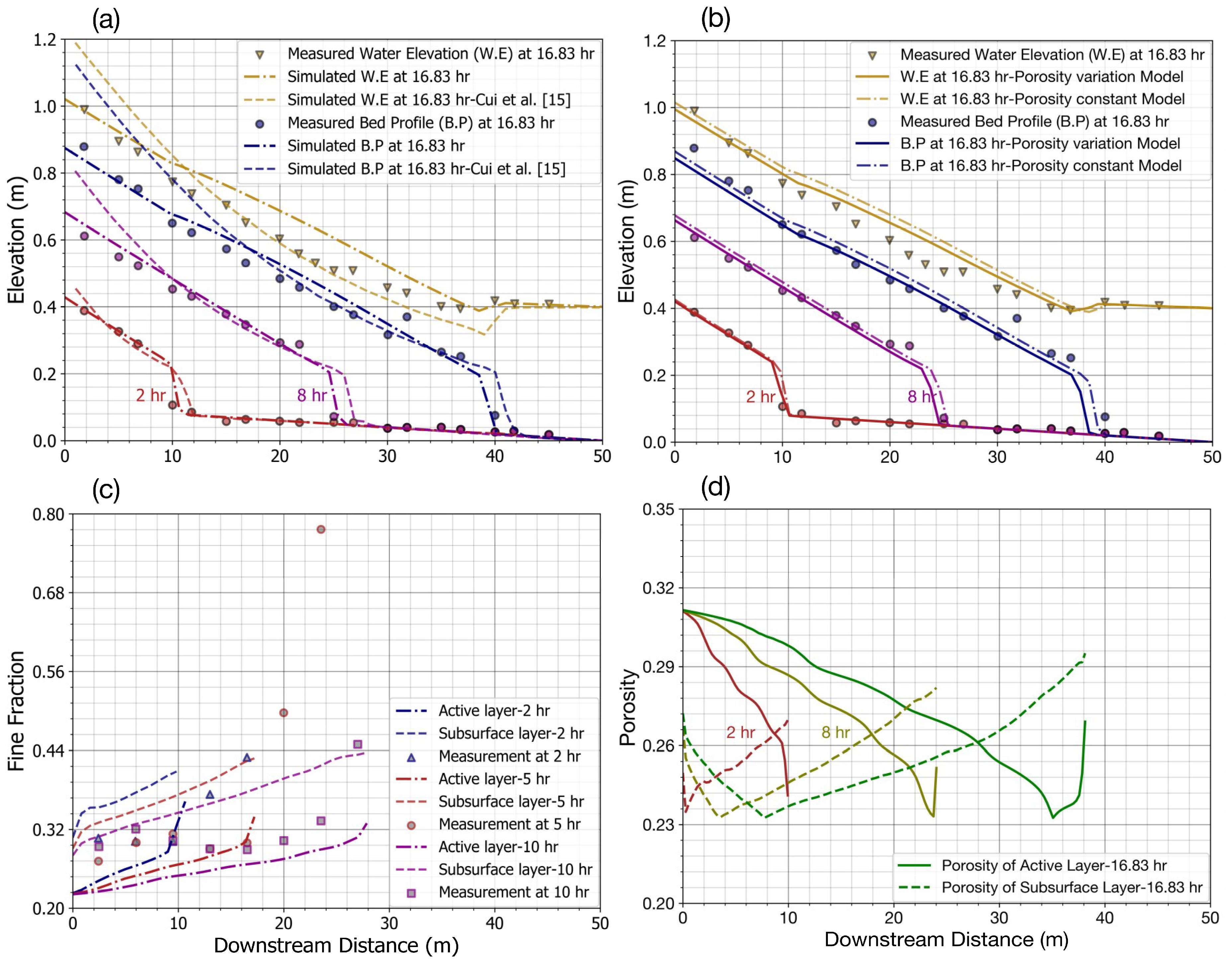
Bed profile due to sediment transport and sediment exchange between the surface layer and subsurface layer is presented in Figure 13 for comparing with the experimental and simulation results of Cui et al. [15] (Figure 13a). The variable porosity model was also compared with our constant model (Figure 13b). It can be seen in Figure 13a,b that our results of bed profile that were obtained from both models agree well with the observations at 2 h (red line), 8 h (pink line), and 16.83 h (blue line) simulations. Since, in Cui’s model, porosity was assumed as a constant of 0.3, we used this value for the initial condition in our simulations. The results in Figure 13a shows that our calculated bed profile has a higher correlation with the observations than Cui’s bed profile, especially on the upstream part. The good agreement between our results and experiments suggests that the developed model with a constant porosity could be adequately satisfied for applying in this study case with low water discharge and week turbulent flow. Further, it can be seen in Figure 13b and Table 5 that the variable porosity model provides slightly better results than those in the constant porosity models. Generally, the bed profile that was obtained from the variable porosity model provides a slightly better agreement with the observation and lower values than those in the constant porosity model. This can be explained that porosity in the active layer and sub-layer tend to change in inverse directions. As a result, the total effect of porosity unsubstantially contributes to bed elevation. Figure 13c,d present the calculated fine fractions and bed porosities in the active and subsurface layers.
Figure 13c shows the result of constant porosity model for the variation of the sand fraction in the surface layer and subsurface layer. The predicted results are compared with the results of the experiment and Cui simulations [15]. The simulated results of two layers for sand fraction variation are unable to be clearly compared with the result of one layer (total bed) of the Cui simulation and experiment. However, from the obtained results, we can realize that the trend of sand fraction variation in two-layer results is suitable with the variation of experimental results. The results of sand fraction variation that were obtained from the constant and variable porosity models will be compared with each other.
Figure 13c shows the fine fraction in the active layer and sublayer at 2 h, 5 h, and 10 h. Fine fraction, as calculated by the variable porosity model at different time experiments, is increased along with space (flume) and time. These results are suitable for the tendency of experiments with a lower value upstream and gradually increasing downstream. For example, the fine fraction is varied from 0.20 to 0.40 along the flume in the active layer and 0.30 to 0.44 in sublayer. The predicted results are also in line with the conclusions of previous studies [15,41]
Figure 13d shows the porosity change at different times of 2 h, 8 h, and 16.83 h for the active layer (solid line) and sub-layer (dash line). Porosity upstream on the surface layer is higher than those downstream, while porosity in the sub-layer tends to increase after reaching the minimum value of 0.24, which is correlated with the gravel fraction and fine fraction, is 0.69 and 0.31, respectively. The variation in porosity gravel-bed is significant, porosity in the active layer varies in range 0.24 to 0.31 and from 0.24 to 0.30 for sublayer.
The porosity of the active layer upstream is reaching its maximum value due to high velocity and gradually reducing because flow velocity decreased along the flume. However, a sudden reduction of velocity on the last part of downstream leads to a rapid increase in fine sediment. When a fine fraction is over the value of 0.31, then the porosity also rises from 0.24 to 0.27 in the active layer. In contrast to the active layer, porosity in sub-layer is not affected by flow velocity—high values of porosity on the upstream and downstream and reaching minimum value of 0.23, as described by the dash lines in Figure 13d.
4. Conclusions
A profound understanding of the phenomenon of natural sediment transport in the gravel-bed river is critical to river management and eco-hydraulics. Due to the complexity of the structure of the river bed and the mechanism of particles movements, most of conventional models simulate sediment transport and bed variation, but they are still limited by various assumptions. The proposed model in this study comes with bed porosity variability and takes the vertical fine sediment transport between multiple layers to assess bed elevation variations, disturbance, and grain sorting into account. In addition, we developed a new model for gravel-bed variation not only by adding a porosity to the Exner’s equation but also by calculating size fraction on the surface layer and subsurface layer by taking into account the exchange rate of fine sediment, porosity variation in the multi-layer. Furthermore, the Discrete Element Method (DEM) was successfully applied to simulate infiltration processes of sediment particles into gravel-bed and effectively investigated the exchange of sediment between the surface layer and sub-layers, including grain size distribution and porosity changes. As a next step, the results that were obtained from the DEM model for different hydro-morphological conditions will be used with data-driven techniques (e.g., Artificial Neural Network) to improve the exchange rate function. Our new bed variation model was verified by testing with the data from three cases, one numerical simulation, and two previous experiments. The results indicated that our model can be applied for simulating bed variations of both constant and variable porosity in gravel-bed rivers. The mode concept is testing and validated for other complicated flow conditions (2D and 3D) with bed-load and suspended-load transport. For this purpose, the new developed model is integrated into the TELEMAC-MASCARET system. Finally, the application of this model system will help stakeholders and managers to effectively maintain fine sediment that is stored in the river bed and to assess the effect of void spaces in gravel on living aquatic insects for eco-hydraulic management.
Author Contributions
V.H.B. designed the study, processed and analyzed the data, developed the models, interpreted the results and wrote the paper. The study has been carried out under the supervision of M.D.B. and P.R., who contributed to the model development stage with theoretical considerations and practical guidance, assisted in the interpretations and integration of the results and helped in preparation of this paper with proof reading and corrections.
Funding
This research was funded by the Vietnam International Education Development (VIED) Scholarship.
Acknowledgments
The contents of this paper are solely the liability of the authors and under no circumstances may be considered as a reflection of the position of the VIED Scholarship. The German Research Foundation (DFG) and the Technical University of Munich (TUM) supported this work in the framework of the Open Access Publishing Program. We much appreciate their help. Special thanks to TUM English Coaching Program for valuable supports and comments to improve this paper. We thank the editor and four anonymous reviewers for their constructive comments, which helped us to improve the manuscript.
Conflicts of Interest
The authors declare no potential conflict of interest.
References
- Dietrich, W.E.; Kirchner, J.W.; Ikeda, H.; Iseya, F. Sediment supply and the development of the coarse surface layer in gravel-bedded rivers. Nature 1989, 340, 215. [Google Scholar] [CrossRef]
- Wilcock, P.R.; DeTemple, B.T. Persistence of armor layers in gravel-bed streams. Geophys. Res. Lett. 2005, 32. [Google Scholar] [CrossRef] [Green Version]
- Cui, Y.; Wooster, J.K.; Baker, P.F.; Dusterhoff, S.R.; Sklar, L.S.; Dietrich, W.E. Theory of fine sediment infiltration into immobile gravel bed. J. Hydraul. Eng.-ASCE 2008, 134, 1421–1429. [Google Scholar] [CrossRef]
- Gibson, S.; Abraham, D.; Heath, R.; Schoellhamer, D. Bridging Process Threshold for Sediment Infiltrating into a Coarse Substrate. J. Geotech. Geoenviron. Eng. 2010, 136, 402–406. [Google Scholar] [CrossRef]
- Schälchli, U. The clogging of coarse gravel river beds by fine sediment. Hydrobiologia 1992, 235, 189–197. [Google Scholar] [CrossRef]
- Wu, F.-C.; Huang, H.-T. Hydraulic resistance induced by deposition of sediment in porous medium. J. Hydraul. Eng. 2000, 126, 547–551. [Google Scholar] [CrossRef]
- Domenico, P.A.; Schwartz, F.W. Physical and Chemical Hydrogeology; Wiley: New York, NY, USA, 1998; Volume 506. [Google Scholar]
- Selby, M.J.; Hodder, A.P.W. Hillslope Materials and Processes; Oxford University Press: Oxford, UK, 1993. [Google Scholar]
- Frings, R.M.; Schuttrumpf, H.; Vollmer, S. Verification of porosity predictors for fluvial sand-gravel deposits. Water Resour Res. 2011, 47. [Google Scholar] [CrossRef]
- Frings, R.M.; Kleinhans, M.G.; Vollmer, S. Discriminating between pore-filling load and bed-structure load: A new porosity-based method, exemplified for the river Rhine. Sedimentology 2008, 55, 1571–1593. [Google Scholar] [CrossRef]
- Verstraeten, G.; Poesen, J. Variability of dry sediment bulk density between and within retention ponds and its impact on the calculation of sediment yields. Earth Surf. Process. Landf. 2001, 26, 375–394. [Google Scholar] [CrossRef]
- Wilcock, P.R. Two-fraction model of initial sediment motion in gravel-bed rivers. Sciences 1998, 280, 410–412. [Google Scholar] [CrossRef]
- Gayraud, S.; Philippe, M. Influence of Bed-Sediment Features on the Interstitial Habitat Available for Macroinvertebrates in 15 French Streams. Int. Rev. Hydrobiol. 2003, 88, 77–93. [Google Scholar] [CrossRef]
- Toro-Escobar, C.M.; Parker, G.; Paola, C. Transfer function for the deposition of poorly sorted gravel in response to streambed aggradation. J. Hydraul. Res. 1996, 34, 35–53. [Google Scholar] [CrossRef]
- Cui, Y. The Unified Gravel-Sand (TUGS) Model: Simulating Sediment Transport and Gravel/Sand Grain Size Distributions in Gravel-Bedded Rivers. Water Resour Res. 2007, 43. [Google Scholar] [CrossRef]
- Sulaiman, M.; Tsutsumi, D.; Fujita, M. Bed variation model considering porosity change in riverbed material. J. Jpn. Soc. Eros. Control Eng. 2007, 60, 11–18. [Google Scholar]
- Parker, G. 1D Sediment Transport Morphodynamics with Applications to Rivers and Turbidity Currents. 2004. Available online: http://hydrolab.illinois.edu/people/parkerg/morphodynamics_e-book.htm (accessed on 14 January 2019).
- Cui, Y.; Parker, G. A quasi-normal simulation of aggradation and downstream fining with shock fitting. Int. J. Sediment Res. 1997, 12, 68–82. [Google Scholar]
- Chiu, Y.-J.; Lee, H.-Y.; Wang, T.-L.; Yu, J.; Lin, Y.-T.; Yuan, Y.J.W. Modeling Sediment Yields and Stream Stability Due to Sediment-Related Disaster in Shihmen Reservoir Watershed in Taiwan. Water 2019, 11, 332. [Google Scholar] [CrossRef]
- Petti, M.; Bosa, S.; Pascolo, S.J.W. Lagoon sediment dynamics: A coupled model to study a medium-term silting of tidal channels. Water 2018, 10, 569. [Google Scholar] [CrossRef]
- Bui, M.D.; Rutschmann, P. Numerical investigation of hydro-morphological changes due to training works in the Salzach River. In River Flow 2012; Taylor and Francis Group: London, UK, 2012; Volumes 1–2, pp. 589–594. [Google Scholar]
- Wilcock, P.R.; Crowe, J.C. Surface-based transport model for mixed-size sediment. J. Hydraul. Eng. 2003, 129, 120–128. [Google Scholar] [CrossRef]
- Leonardson, R. Exchange of Fine Sediments with Gravel Riverbeds. Ph.D. Thesis, University of California, Berkeley, CA, USA, 2010. [Google Scholar]
- Wooster, J.K.; Dusterhoff, S.R.; Cui, Y.T.; Sklar, L.S.; Dietrich, W.E.; Malko, M. Sediment supply and relative size distribution effects on fine sediment infiltration into immobile gravels. Water Resour. Res. 2008, 44. [Google Scholar] [CrossRef] [Green Version]
- Gibson, S.; Abraham, D.; Heath, R.; Schoellhamer, D. Vertical gradational variability of fines deposited in a gravel framework. Sedimentology 2009, 56, 661–676. [Google Scholar] [CrossRef]
- Bui, M.D.; Rutschmann, P. Numerical modelling of non-equilibrium graded sediment transport in a curved open channel. Comput. Geosci. 2010, 36, 792–800. [Google Scholar] [CrossRef]
- Cundall, P.A.; Strack, O.D. A discrete numerical model for granular assemblies. Geotechnique 1979, 29, 47–65. [Google Scholar] [CrossRef]
- Johnson, K.L. Contact Mechanics; Cambridge University Press: Cambridge, UK, 1985. [Google Scholar]
- Church, M. River bed gravels: Sampling and analysis. In Sediment Transport in Gravel-Bed Rivers; Wiley: Hoboken, NJ, USA, 1987; pp. 43–78. [Google Scholar]
- Bui, M.D.; Bui, V.H.; Rutschmann, P. A new concept for modelling sediment transport in gravel bed rivers. In Proceedings of the 21st Vietnam Fluid Mechanics, Quynhon, Vietnam, 10–13 December 2018. (In Vietnamese). [Google Scholar]
- Nunez-Gonzalez, F.; Martin-Vide, J.P.; Kleinhans, M.G. Porosity and size gradation of saturated gravel with percolated fines. Sedimentology 2016, 63, 1209–1232. [Google Scholar] [CrossRef] [Green Version]
- Koltermann, C.E.; Gorelick, S.M. Fractional packing model for hydraulic conductivity derived from sediment mixtures. Water Resour Res. 1995, 31, 3283–3297. [Google Scholar] [CrossRef]
- Kamann, P.J.; Ritzi, R.W.; Dominic, D.F.; Conrad, C.M. Porosity and permeability in sediment mixtures. Groundwater 2007, 45, 429–438. [Google Scholar] [CrossRef]
- Yu, A.B.; Standish, N. Limitation of Proposed Mathematical-Models for the Porosity Estimation of Nonspherical Particle Mixtures. Ind. Eng. Chem. Res. 1993, 32, 2179–2182. [Google Scholar] [CrossRef]
- Yu, A.B.; Standish, N. Estimation of the Porosity of Particle Mixtures by a Linear-Mixture Packing Model. Ind. Eng. Chem. Res. 1991, 30, 1372–1385. [Google Scholar] [CrossRef]
- Zhang, H.; Makse, H. Jamming transition in emulsions and granular materials. Phys. Rev. E. 2005, 72, 011301. [Google Scholar] [CrossRef]
- Kenney, T.; Chahal, R.; Chiu, E.; Ofoegbu, G.; Omange, G.; Ume, C. Controlling constriction sizes of granular filters. Can. Geotech. J. 1985, 22, 32–43. [Google Scholar] [CrossRef]
- Indraratna, B.; Locke, M. Design methods for granular filters—Critical review. Proc. Inst. Civ. Eng. -Geotech. Eng. 1999, 137, 137–147. [Google Scholar] [CrossRef]
- Sulaiman, M.; Tsutsumi, D.; Fujita, M. Porosity of sediment mixtures with different type of grain size distribution. Annu. J. Hydraul. Eng. 2007, 51, 133–138. [Google Scholar] [CrossRef]
- Paola, C.; Parker, G.; Seal, R.; Sinha, S.K.; Southard, J.B.; Wilcock, P.R. Downstream fining by selective deposition in a laboratory flume. Science 1992, 258, 1757–1760. [Google Scholar] [CrossRef]
- Toro-Escobar, C.M.; Paola, C.; Parker, G.; Wilcock, P.R.; Southard, J.B. Experiments on downstream fining of gravel. II: Wide and sandy runs. J. Hydraul. Eng. 2000, 126, 198–208. [Google Scholar] [CrossRef]
- Seal, R.; Paola, C.; Parker, G.; Southard, J.B.; Wilcock, P.R. Experiments on downstream fining of gravel: I. Narrow-channel runs. J. Hydraul. Eng. 1997, 123, 874–884. [Google Scholar] [CrossRef]
- Seal, R.; Parker, G.; Paola, C.; Mullenbach, B. Laboratory Experiments on Downstream Fining of Gravel, Narrow Channel Runs 1 through 3: Supplemental Methods and Data; External Memorandum M-239; St. Anthony Fall Anthony Falls Hydraulic Laboratory, University of Minnesota: Minneapolis, MN, USA, 1995. [Google Scholar]
Figure 1.
Porosity variation of grain system due to fine grain exchange.

Figure 2.
The structure diagram of the vertical cross-section is based on the multi-layers model. (1) = active layer; (2) and (3) = substrate layers; Ea and Em = Active layer thickness and active-stratum layer thickness; zb = bed elevation; zc and zd = substrate elevations.
Figure 2.
The structure diagram of the vertical cross-section is based on the multi-layers model. (1) = active layer; (2) and (3) = substrate layers; Ea and Em = Active layer thickness and active-stratum layer thickness; zb = bed elevation; zc and zd = substrate elevations.

Figure 3.
Bed level change due to porosity variation in different time steps.

Figure 4.
Schematic structure of bottom sediments as a function dependent on the magnitude of the fine component sediment.
Figure 4.
Schematic structure of bottom sediments as a function dependent on the magnitude of the fine component sediment.

Figure 5.
Classifying the mixture to partial specific volumes for diameter dj.

Figure 6.
The structure of bed gravel and fine sediment distribution depends on the size ratio (d/D). Left: Fine sediments distribution at a cross-section along the channel at the final computational step with d/D = 0.154 (a), d/D = 0.231(b), and d/D = 0.414 (c); Right: Fine fraction variation in gravel depth with different size ratio.

Figure 7.
(a)—Structure of bed sediments at a cross-section along the channel at the final computational step (b)—Fine fraction distribution at the end of simulation; and, (c)—Bed porosity distribution along the depth at the beginning and the end of the computation time.
Figure 7.
(a)—Structure of bed sediments at a cross-section along the channel at the final computational step (b)—Fine fraction distribution at the end of simulation; and, (c)—Bed porosity distribution along the depth at the beginning and the end of the computation time.

Figure 8.
The performance of bed-porosity variation model in different times (a)—Bed elevation; (b)—Porosity of active-layer; (c)—Coarse size fraction of active-layer; and, (d)—Fine size fraction of active-layer.
Figure 8.
The performance of bed-porosity variation model in different times (a)—Bed elevation; (b)—Porosity of active-layer; (c)—Coarse size fraction of active-layer; and, (d)—Fine size fraction of active-layer.

Figure 9.
Comparison between the conventional model and the new model at the final time step (a)—Porosity of the active-layer; and, (b)—Bed elevation.
Figure 9.
Comparison between the conventional model and the new model at the final time step (a)—Porosity of the active-layer; and, (b)—Bed elevation.

Figure 10.
Schematic drawing of experimental channel and apparatus [16].
Figure 10.
Schematic drawing of experimental channel and apparatus [16].

Figure 11.
Bed variation for surface layer in comparison with observations from flume measurements [16]: (a) bed elevation—erosion case; (b) bed elevation—deposition case (c) Fine fraction variation in erosion and deposition cases; and, (d) Porosity variation in erosion and deposition cases.
Figure 11.
Bed variation for surface layer in comparison with observations from flume measurements [16]: (a) bed elevation—erosion case; (b) bed elevation—deposition case (c) Fine fraction variation in erosion and deposition cases; and, (d) Porosity variation in erosion and deposition cases.

Figure 12.
Flume set up for St. Anthony Falls Laboratory (SAFL) downstream fining experiments [15].
Figure 12.
Flume set up for St. Anthony Falls Laboratory (SAFL) downstream fining experiments [15].

Figure 13.
Simulated results in comparison with possible observations and Cui’s study [15]: (a) bed and water elevations obtained from constant porosity model; (b) bed and water elevations obtained from both constant and variable porosity models; (c) Sand fraction obtained from variable porosity model; and, (d) Calculated porosity variation.


Table 1.
Parameters for numerical simulation.
| Density of Sphere (kg/m3) | Density of Water (kg/m3) | Young’s Modulus (Pa) | Poisson Ratio | Friction Between Grains | Coefficient of Restitution |
|---|---|---|---|---|---|
| 2700 | 1000 | 5.0 × 10⁶ | 0.45 | 0.5 | 0.4 |
Table 2.
Experimental conditions for two runs, where: qw—water discharge; qs—sediment discharge; Fr—Froude number; τ—non-dimensional bed shear stress [16].
Table 2.
Experimental conditions for two runs, where: qw—water discharge; qs—sediment discharge; Fr—Froude number; τ—non-dimensional bed shear stress [16].
| Exp. | qw (m2/s) | qs × 10−6 (m2/s) | h (m) | v (m/s) | Fr | τ (Fine) | τ (Coarse) |
|---|---|---|---|---|---|---|---|
| Run-1 Run-2 | 0.034 0.034 | 0 31.8 | 0.039 0.045 | 0.879 0.754 | 1.428 1.133 | 0.178 0.203 | 0.026 0.030 |
Table 3.
Statistical performances of bed variation model within surface layer.
| Erosion | Deposition | |||||
|---|---|---|---|---|---|---|
| Variation | Constant | Sulaiman | Variation | Constant | Sulaiman | |
| Bed Elevation | ||||||
| R | 0.99510 | 0.99442 | 0.99412 | 0.99451 | 0.99538 | 0.99465 |
| RMSE | 0.00585 | 0.00631 | 0.00560 | 0.00347 | 0.00490 | 0.00414 |
| MAE | 0.00451 | 0.00546 | 0.00442 | 0.00275 | 0.00424 | 0.00343 |
| Fine Fraction | ||||||
| R | 0.98936 | 0.98953 | 0.99124 | 0.96269 | 0.98205 | 0.96953 |
| RMSE | 0.16423 | 0.17410 | 0.26149 | 0.07897 | 0.09265 | 0.07297 |
| MAE | 0.12371 | 0.12518 | 0.18397 | 0.05929 | 0.08579 | 0.05088 |
Table 4.
Parameters for SAFL Downstream Fining Experiments; where: qw—water discharge, qs—sediment discharge, ξd—downstream water depth, S0—flume slope, fs—sand fraction [15].
Table 4.
Parameters for SAFL Downstream Fining Experiments; where: qw—water discharge, qs—sediment discharge, ξd—downstream water depth, S0—flume slope, fs—sand fraction [15].
| Exp. | qw (m2/s) | qs (m2/s) | ξd (m) | S0 (%) | fs % | Time (h) |
|---|---|---|---|---|---|---|
| Run 1 | 0.163 | 2.37 × 10⁻⁴ | 0.4 | 0.20 | 33 | 2, 8, 16.83 |
Table 5.
Statistical performances of bed variation model in two layers.
| 2 h | 8 h | 16 h | |||||||
|---|---|---|---|---|---|---|---|---|---|
| R | RMSE | MAE | R | RMSE | MAE | R | RMSE | MAE | |
| Variation | 0.987 | 0.019 | 0.010 | 0.998 | 0.016 | 0.013 | 0.989 | 0.033 | 0.027 |
| Constant | 0.980 | 0.023 | 0.011 | 0.996 | 0.024 | 0.018 | 0.988 | 0.034 | 0.032 |
© 2019 by the authors. Licensee MDPI, Basel, Switzerland. This article is an open access article distributed under the terms and conditions of the Creative Commons Attribution (CC BY) license (http://creativecommons.org/licenses/by/4.0/).
Share and Cite
MDPI and ACS Style
Bui, V.H.; Bui, M.D.; Rutschmann, P. Advanced Numerical Modeling of Sediment Transport in Gravel-Bed Rivers. Water 2019, 11, 550. https://doi.org/10.3390/w11030550
AMA Style
Bui VH, Bui MD, Rutschmann P. Advanced Numerical Modeling of Sediment Transport in Gravel-Bed Rivers. Water. 2019; 11(3):550. https://doi.org/10.3390/w11030550
Chicago/Turabian StyleBui, Van Hieu, Minh Duc Bui, and Peter Rutschmann. 2019. "Advanced Numerical Modeling of Sediment Transport in Gravel-Bed Rivers" Water 11, no. 3: 550. https://doi.org/10.3390/w11030550
Note that from the first issue of 2016, this journal uses article numbers instead of page numbers. See further details here.