A Performance Comparison of Machine Learning Algorithms for Arced Labyrinth Spillways


1
International Centre for Numerical Methods in Engineering (CIMNE), Universitat Politècnica de Catalunya, 08034 Barcelona, Spain
2
Department of Civil and Environmental Engineering, Utah Water Research Laboratory, Utah State University, Logan, UT 84321, USA
*
Author to whom correspondence should be addressed.
Water 2019, 11(3), 544; https://doi.org/10.3390/w11030544
Submission received: 29 January 2019
/
Revised: 8 March 2019
/
Accepted: 13 March 2019
/
Published: 16 March 2019
(This article belongs to the Special Issue Machine Learning Applied to Hydraulic and Hydrological Modelling)
Abstract
:Labyrinth weirs provide an economic option for flow control structures in a variety of applications, including as spillways at dams. The cycles of labyrinth weirs are typically placed in a linear configuration. However, numerous projects place labyrinth cycles along an arc to take advantage of reservoir conditions and dam alignment, and to reduce construction costs such as narrowing the spillway chute. Practitioners must optimize more than 10 geometric variables when developing a head–discharge relationship. This is typically done using the following tools: empirical relationships, numerical modeling, and physical modeling. This study applied a new tool, machine learning, to the analysis of the geometrically complex arced labyrinth weirs. In this work, both neural networks (NN) and random forests (RF) were employed to estimate the discharge coefficient for this specific type of weir with the results of physical modeling experiments used for training. Machine learning results are critiqued in terms of accuracy, robustness, interpolation, applicability, and new insights into the hydraulic performance of arced labyrinth weirs. Results demonstrate that NN and RF algorithms can be used as a unique expression for curve fitting, although neural networks outperformed random forest when interpolating among the tested geometries.
1. Introduction
1.1. Problem Statement
Water is an unevenly distributed global resource. Many communities rely heavily on water distribution systems and key elements in that system—hydraulic structures—for water supply and flood control. These communities range in size and demand, from small agrarian pueblos (e.g., areas in northern Peru, southern Africa, eastern Asia) to large metropolises (e.g., Las Vegas would not exist without Hoover Dam) [1]. Water sources may be within a short walk, or as far as many kilometers away with mountains in between. Furthermore, communities require infrastructure such as dams and levees to store precipitation in dry periods and to provide flood protection in periods of excess [2]. These water systems often include flow control structures such as weirs and spillways that may be located in canals, channels, rivers, and reservoirs.
The primary performance metric for many of these control structures is the relationship between energy head (i.e., an elevation or depth) and discharge. Significant funds are expended every year analyzing hydrologic and hydraulic risks. These efforts frequently include updating head–discharge relationships of existing flow-control structures or designing new structures that meet specified head–discharge performance criteria. Therefore, it is vital to leverage appropriate technologies to meet water infrastructure demands by supporting these analyses and efforts.
1.2. Labyrinth Weirs
A labyrinth weir is a free-overfall control structure that is folded in plan to create a repeating triangular, trapezoidal, rectangular, or even circular pattern (i.e., cycle), although the commonly constructed type is the trapezoidal labyrinth weir. Labyrinth weirs offer several performance advantages compared to other types of hydraulic structures; they typically require no operation, little maintenance, and can be less expensive to construct compared to other dam rehabilitation options [3]. Furthermore, the geometry may be tailored to a specific site. Also, these types of weirs may pass more flow for a given head and channel width relative to other linear weirs due to the additional crest length.
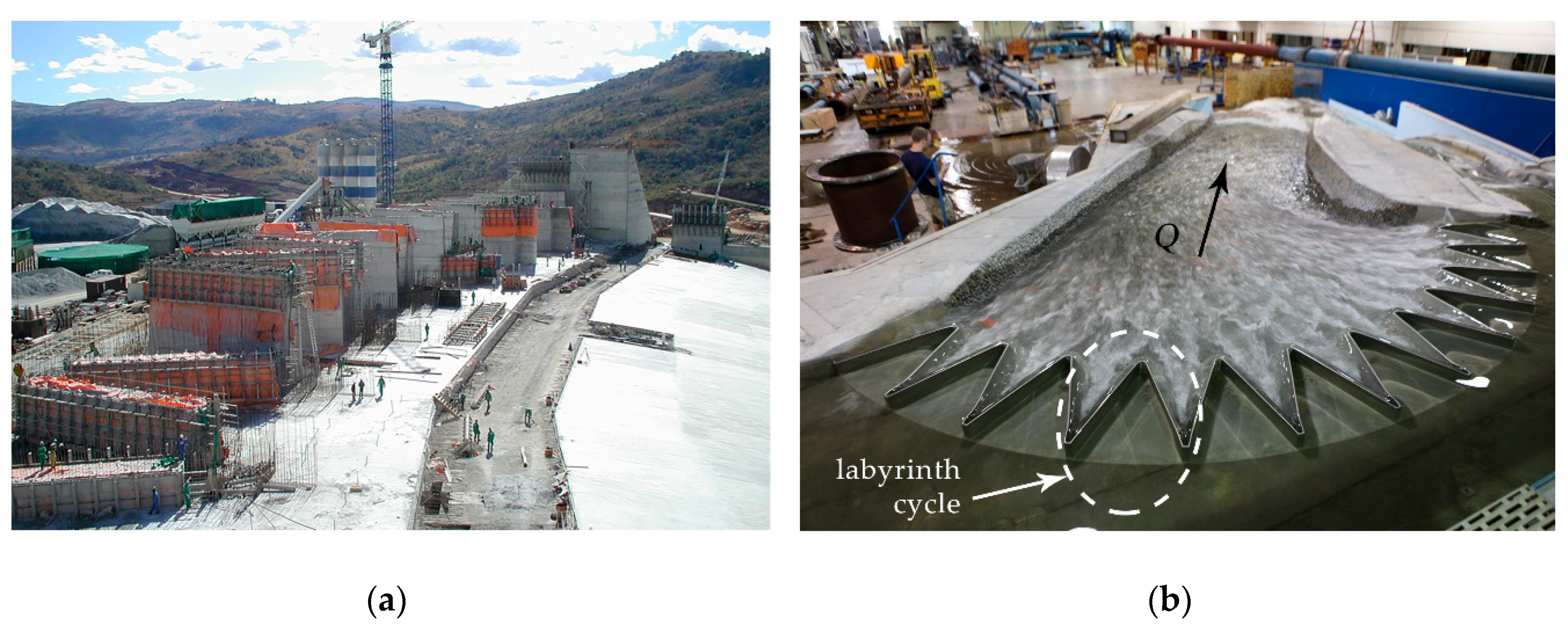
Various aspects of labyrinth weirs were studied during the past 60 years, including the head–discharge performance of many geometries (e.g., References [4,5,6,7,8,9,10,11]), scale effects [12,13], energy dissipation [14,15], and effects of floating debris [16,17]. The cycles of labyrinth weirs are typically placed in a linear configuration. However, some projects place labyrinth cycles along an arc to take advantage of reservoir conditions and dam alignment, and to reduce construction costs such as by narrowing the spillway chute (e.g., Isabella Dam (model shown in Figure 1b), Maria Cristina Dam, Kizilcapinar Dam, and Maguga Dam (see Figure 1a)). These efforts corresponded to several studies conducted in laboratories on arced labyrinth weirs [6,18,19,20,21,22,23,24]. A challenge with arced labyrinth weirs is the large number of geometric parameters and hydraulic factors that influence discharge capacity. The geometric layout and experimental data by Reference [8] provide a basis for additional analyses of the hydraulic performance of arced labyrinth weirs using various numerical approaches such as empirical relationships, computational fluid dynamics, and machine learning (ML).
1.3. Machine Learning
The development of sensors and communications made available enormous volumes of data of civil engineering systems that could be useful for their improvement [25]. The analysis of these data requires specific tools that were developed in recent years in the field of computer science, since a potential significant challenge is analyzing the data to identify dominant relationships and make accurate predictions. In parallel, ML algorithms capable of addressing different types of problems were proposed and applied to a variety of tasks, which can be grouped fundamentally in regression and classification. These tools have a great potential of application to solve other engineering problems for which physical or statistical models were traditionally used.
The main feature of these models is that they are not based on physics but only rely on available data. Therefore, they can be very useful in systems where there is uncertainty in the processes involved or it is difficult to apply physics-based mathematical expressions, provided that enough information (i.e., sufficient data of the system) for various scenarios is available. Thus, neural networks (NNs) were used for years in hydrology to model rainfall–runoff processes and predict flooding (e.g., References [26,27,28]). In dam safety, there is also a growing community of researchers that employ various algorithms to estimate the structural response of a dam based on the acting loads and to detect anomalies [29,30,31,32,33]. Other fields of application in hydraulic engineering include the management of water supply networks [34] and velocity estimation in air–water flows [35]. In hydraulic engineering, these techniques are also used in problems analogous to that proposed in this paper. For example, Reference [36] used NNs to obtain an expression to estimate the discharge capacity of Piano Key Weirs, a special type of labyrinth weir that has rectangular cycles, overhangs, and ramps in each cycle. Emiroglu and Kisi published a comparison between NNs and adaptive neuro fuzzy inference systems (ANFIS) for an analogous case in labyrinth side weirs [37]. Several ML techniques were compared by Azamathulla et al. [38] to predict the discharge coefficient of linear side weirs, and NNs were also used to analyze the discharge capacity of radial-gated spillways [39].
NNs are the most commonly used machine learning technique in hydraulic engineering. As illustrated, there are numerous publications with examples of applications and methodological considerations on the training process, which, in this case, include the training algorithm and parameters, as well as the network architecture (number of layers and neurons per layer). In some instances, NN-based models were found to be more accurate than conventional statistical approaches to estimate system response, while providing additional benefits such as their capability to model non-linear relationships in a straightforward way (e.g., Reference [40]).
Nonetheless, NNs also feature certain drawbacks such as the lack of a unified criterion to determine network architecture, the dependence on the initialization of the weights, and the need for normalizing inputs [41].
Ensemble models based on decision trees such as random forests (RFs) and boosted regression trees (BRTs) were also applied in similar settings, and offer some interesting features [41,42] such as the following:
- They are robust against the presence of uninformative or highly correlated inputs, which are automatically neglected during model training.
- They can handle numerical and categorical predictors with little pre-processing.
- They are less prone to overfitting than other ML algorithms.
- They account for input interaction.
In this work, both NNs and RFs were employed to estimate the discharge coefficient of arced labyrinth weirs, based on the results of experiments [8]. The main objectives of this study were as follows:
- Obtaining a unique function for estimating the discharge coefficient in terms of the geometric features and the headwater ratio (H/P);
- Comparing the results obtained with both ML algorithms in terms of the following:
- ○
- Accuracy;
- ○
- Robustness;
- ○
- Interpolation;
- ○
- Possibilities to draw conclusions on the system performance from model interpretation;
- ○
- Applicability.
2. Experimental Approach
2.1. Physical Modeling
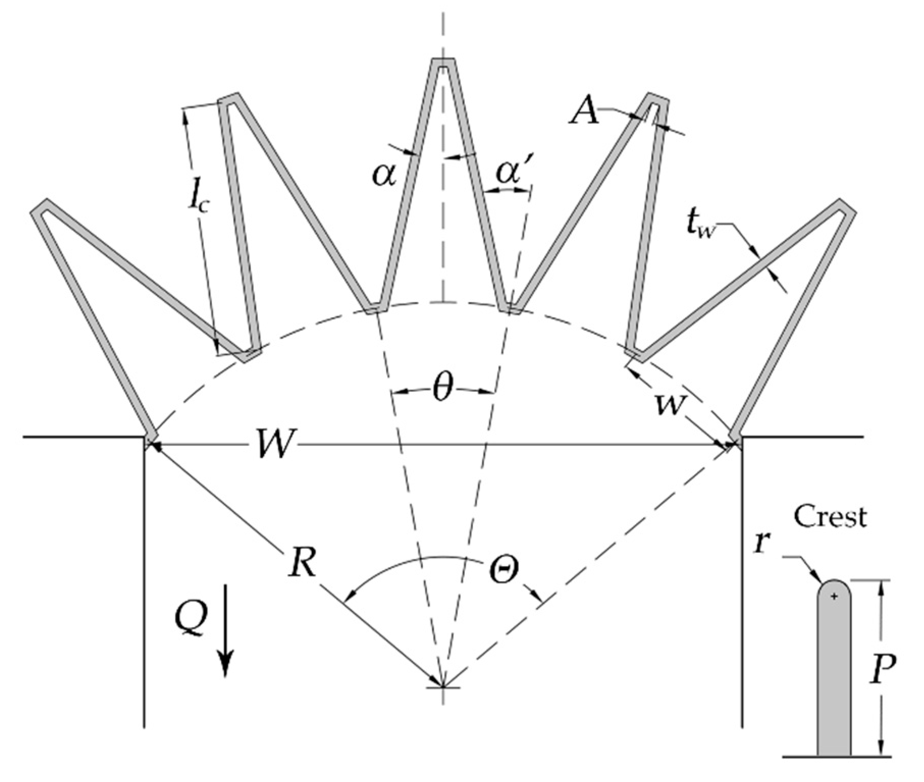
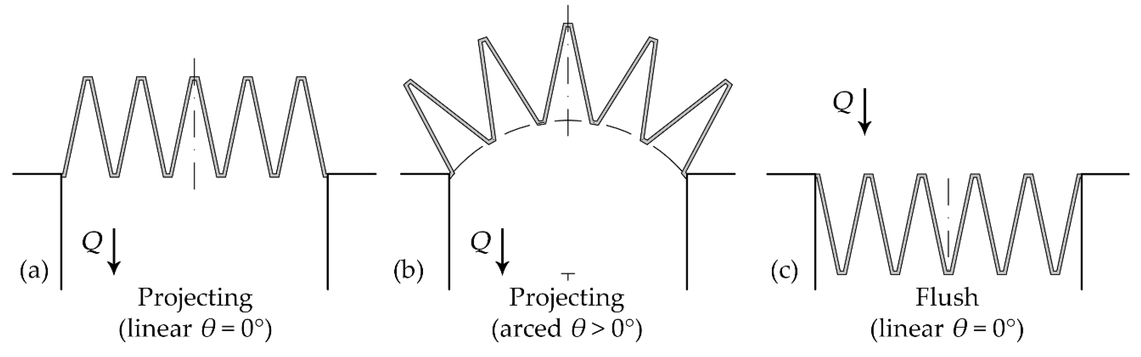
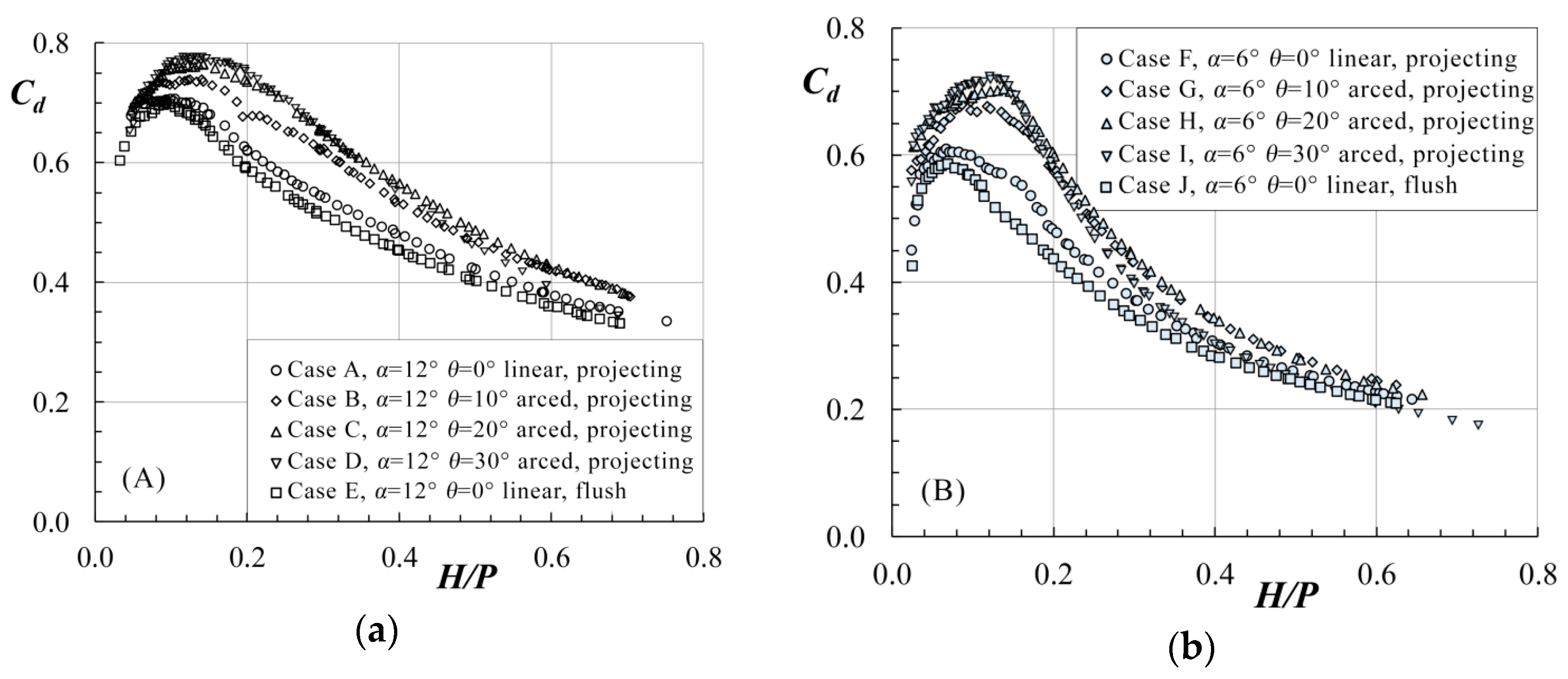
Physical modeling of labyrinth spillways was conducted at the Utah Water Research Laboratory (UWRL) in Utah, USA. An overview of arced labyrinth weir parameters is presented in Figure 2 and tested reservoir configurations are presented in Figure 3. The experimental test matrix is summarized in Table 1. Experiments were conducted in a 7.3 m by 6.7 m rectangular headbox with a depth of 1.5 m to simulate reservoir conditions. Flow was introduced into the reservoir via a diffuser pipe along three walls and a baffle system. A free overfall was placed downstream of the arced labyrinth weirs. For details of the experimental facilities and set-up including schematics, please see Reference [8]. The labyrinth weirs were 203.2 mm in height (P), with a cycle width (w) of 408 mm, and a wall thickness (tw) of 25.4 mm with a half-round crest shape with radius (r) equivalent to half the weir wall thickness (r = tw/2). All tested weirs were machined from high-density polyethylene without artificial venting or aeration. Flow measurements were performed under steady-state conditions using calibrated orifice plates accurate to ±0.25% and using a datalogger (22-Hz sampling rate). Piezometric head h measurements were performed using point gage instrumentation and a stilling well accurate to ±0.15 mm. A repeatability component was also included in data collection where a minimum of 10% of experiments were repeated. Composite experimental uncertainties varied slightly between each model; for H/P ≈ 0.15, uncertainties were less than 2% and decreased with increasing H/P. As expected, uncertainties increased with decreasing flow depth and were about 5% or less for H/P = 0.05 (h ≈ 10 mm). An additional component of this study was to quantify the approaching flow field in the reservoir to the weirs. This was performed using an acoustic Doppler two-dimensional (2D) velocity probe which confirmed excellent approach conditions and flow symmetry—for additional details, please see Reference [8]. Differences in head–discharge predictions between these models and prototypes (scale effects for Cd) are dependent upon the size of the prototype (specifically the scaling ratio) and H/P with prediction errors anticipated to be −5% or less for H/P > 0.05 [43]. The experimental results are included in Figure 4.
2.2. Estimation of Cd
The head–discharge relationship for an arced labyrinth weir can be described as follows [8,21]:
where Q is the discharge over weir and is dependent on hydraulic and geometric inputs, Cd is a discharge coefficient determined experimentally, Lc-cycle is the centerline length for a single labyrinth weir cycle that includes lc (the centerline length of weir sidewall), N is the number of labyrinth weir cycles, g is the acceleration constant of gravity, H is the unsubmerged total upstream head on the weir, estimated as h + V2/2g, h is the piezometric head relative to the weir crest, V is the average cross-sectional flow velocity upstream of the weir, α is the cycle sidewall angle, α’ is the upstream labyrinth weir sidewall angle, where α’ = α + θ/2, θ is the cycle arc angle, P is the weir height, A is the inside apex width, w the cycle width, W is the width of the channel, R is the arc radius, tw is the thickness of weir wall at the crest, and Θ is the arced labyrinth weir angle.
2.3. Model Fitting
In order to obtain a unique model based on ML to compute the discharge coefficient Cd, the features of the model tests were codified as input variables as described in Table 2:
The experimental data were used in two ways. Firstly, all configurations were considered to build the models that provide a single expression for the estimation of Cd. The prediction accuracy was computed on a validation set including a random 30% of the available data. These models were later used to analyze the interpolation capacity, i.e., the results of the discharge coefficient for intermediate configurations between two of those tested in laboratory.
Subsequently, separate models were fitted considering only Cases A, B, D, E, F, G, I, and J, and leaving C and H for external validation. With this approach it is possible to calculate the real accuracy of the model for these two configurations using experimental data from the laboratory. This case allows estimating the application potential of the ML models to reduce the number of cases to be considered in experimental campaigns. Cases C and H were selected for this purpose because they represent intermediate cases between others tested, with only one parameter modified (α).
All ML models were fitted using the language/programming environment R [44].
2.3.1. Random Forests
A random forest (RF) model is a group of regression (or classification) trees, each of which is trained on modified versions of the training set [42,45]. The overall output is computed as the average of the prediction of each individual tree. The training process of an RF model includes two random components with the aim of capturing as many patterns in the training set as possible while preventing overfitting.
The parameters that govern the training process are (a) the number of trees (ntree) and (b) the number of inputs to consider at each split (mtry). The library randomForestSRC [46] was used with the default number of trees (1000) and mtry = 3. Although both parameters were reported to have little influence on the results [47], preliminary tests showed that mtry > 2 was necessary to achieve stable accuracy. This ensures that at least one of the most influential variables (H/P, α, and θ) is considered at each split. Figure S1 (Supplementary Materials) shows the effect of mtry on prediction accuracy.
The model fit with all cases was subsequently analyzed to identify input effects in the system response. This could be accomplished via two approaches. Firstly, the importance of each input on the response can be estimated by the variable importance measure, which is based on the assumption that the importance of each input is proportional to the increase in error that is registered when the corresponding input is randomly altered. More precisely, the prediction error for the model is computed and stored. Then, the values of one input are randomly shifted; the resulting dataset is supplied to the model, and predictions and accuracy are again computed. If the input is strongly associated with the response, the accuracy will decrease, and vice versa. The same process is repeated for each input, obtaining a quantification of the strength of their importance in the process, as learned by the model. The results are normalized so that they can be compared across inputs.
Secondly, partial dependence plots can be generated. For each variable, equally spaced values are taken along its range; average model prediction is computed for each value while keeping the remaining inputs at their true values. The resulting curve depicts the average effect of each input on system output.
2.3.2. Neural Networks
The nnet library [48] was used for the NN-based model. The categorical variables (i.e., approach configurations) were transformed into numerical values for each categorical variable in the original training set. A numeric value (1–0) was assigned to each according to the corresponding geometry (Table 3). The numeric inputs were centered and scaled before model fitting.
In this relatively simple setting, with a well-known physical process and a reduced number of input variables, good agreement is expected using an NN model with one hidden layer [49] (p. 132). Thus, the architecture of the final model is determined by the number of neurons in that hidden layer. The coefficients and the prediction accuracy depend also on the regularization parameter (weight decay; wd). The best combination of (# neurons, wd) in terms of prediction accuracy was tested. In particular, testing included the following values: 10, 15, 20, 25, and 30 neurons, and 10−3, 10−4, and 10−5 for wd. Default values were used for other options, except for the output units, which were set to use linear functions (linout = TRUE) [48]. The prediction accuracy for each combination was assessed through (three times) repeated fourfold cross-validation, for which the caret library [50] was employed. The effect of both parameters on the prediction accuracy is shown in Figure S2 (Supplementary Materials).
Variable importance in NN models was estimated with the Olden index [51], as implemented in the NeuralNetTools library [52]. It is based on the product of the connection weights between neurons, including their sign, as learned by the model. Therefore, it can be used to assess the overall influence of each input variable in the response of the system. However, it does not allow a direct comparison with the results of the RF model because the calculation procedure and the nature of the models are different and also because of the transformation of the categorical variables performed for the NN model.
The importance of variables generated from categorical inputs (ArcP, Lin, NonLin, Flu, Proj) cannot be interpreted directly. These variables, although technically numerical, indeed take values of 0 or 1, depending on the configuration feature. The effect of each feature on Cd can consequently be analyzed by comparing the importance of the inputs within each group, i.e., those derived from each categorical variable. Thus, to see the effect of the approach (linear/non-linear), the importance of the variables “Lin” and “NonLin” must be compared. The same reasoning can be followed for the variable “App”, which in the NN model is expanded into ArcP, Proj, and Flu (Table 3).
To compare the relative importance of the variables, the following operations were performed on the results of the Olden index:
- For the numerical variables (H/P, α and θ), the absolute values were taken.
- For Lin/NonLin, the difference between Olden importance was considered.
- For ArcP/Proj/Flu, the standard deviation was used.
- The results were scaled to sum to 100.
The pdp library [53] was used to consider partial dependence, where the same procedure (as described previously) was implemented for NN models.
3. Results
3.1. Unique Expression
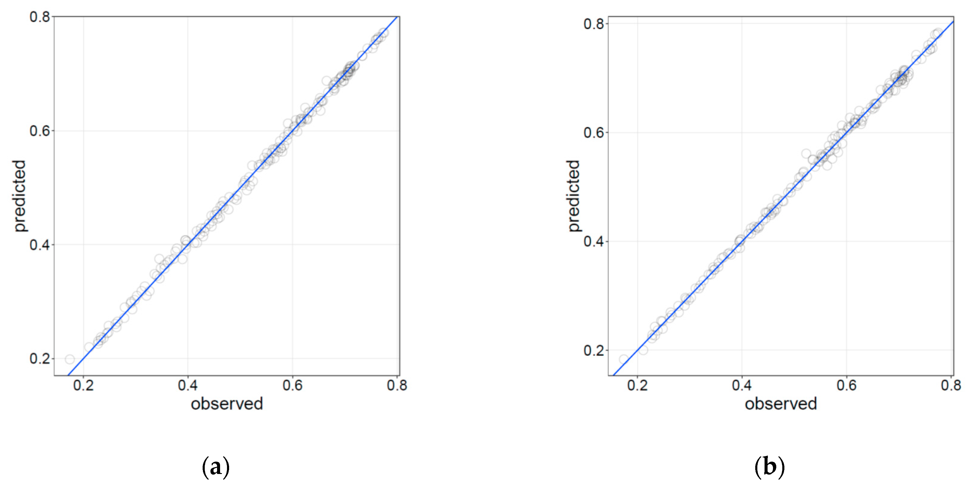
The results for RF- and NN-based models are shown in Figure 5. All available configurations (Table 1) were used to fit these two models. As mentioned above, 30% of the data were randomly taken from the training set to compute the validation accuracy. The plots show the predictions on the abscissa and the observations on the ordinate. Perfect agreement is represented by a straight line starting at (0,0) with slope = 1. Prediction accuracy was quantified by means of some conventional error indexes (Table 4).
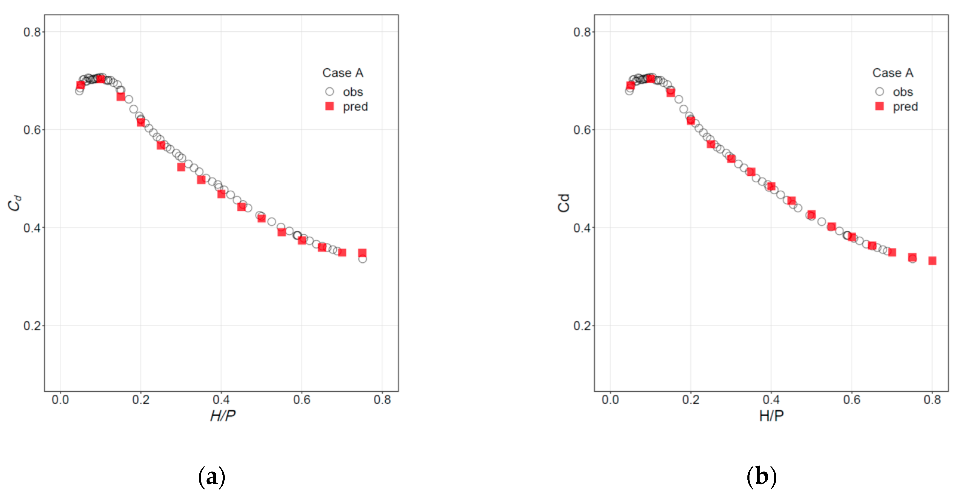
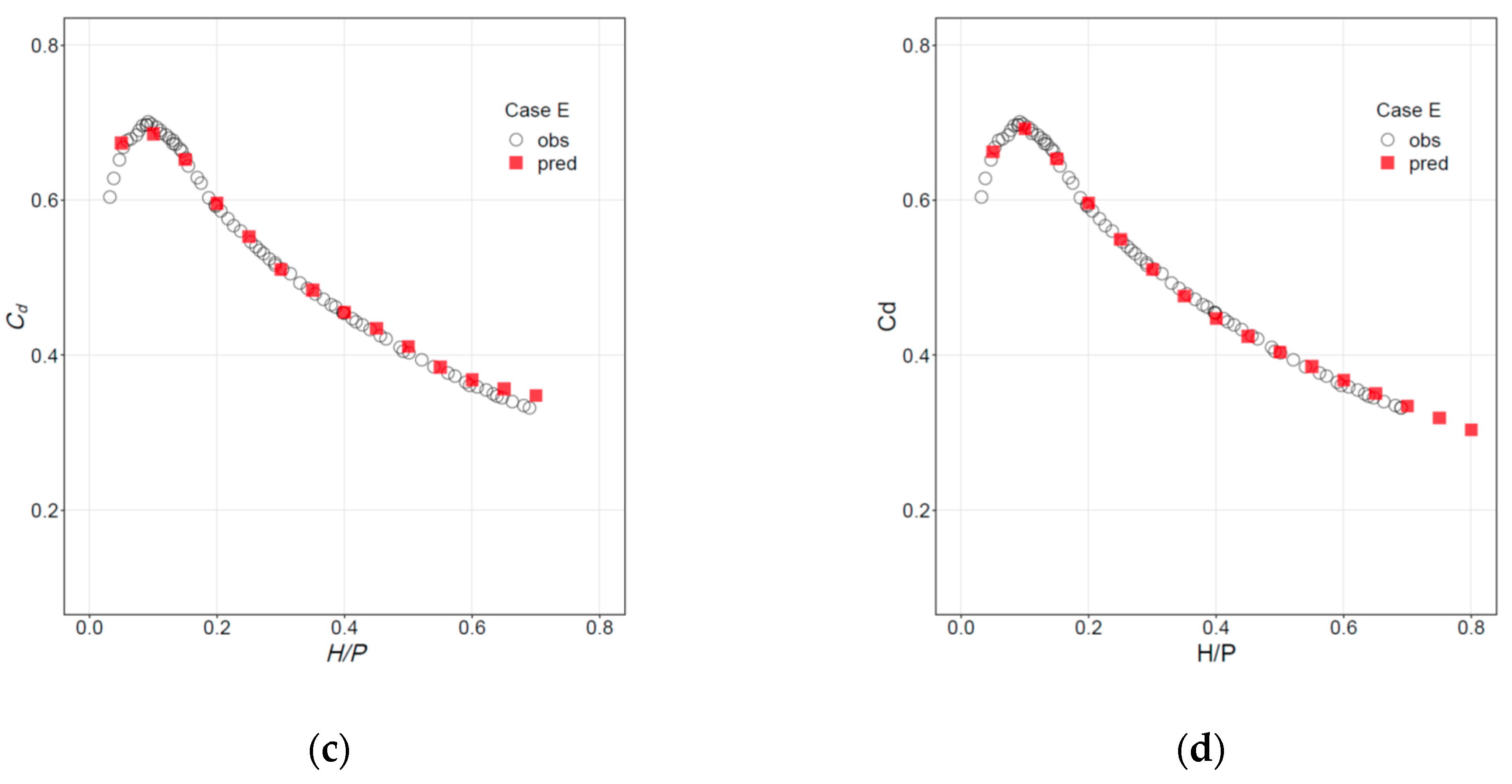
The same results can be presented in the form of discharge curves, with Cd as a function of H/P, as shown in Figure 6 for Cases A and E. Similar plots for the remaining cases are included in Figures S3 and S4 (Supplementary Materials).
3.2. Interpolation
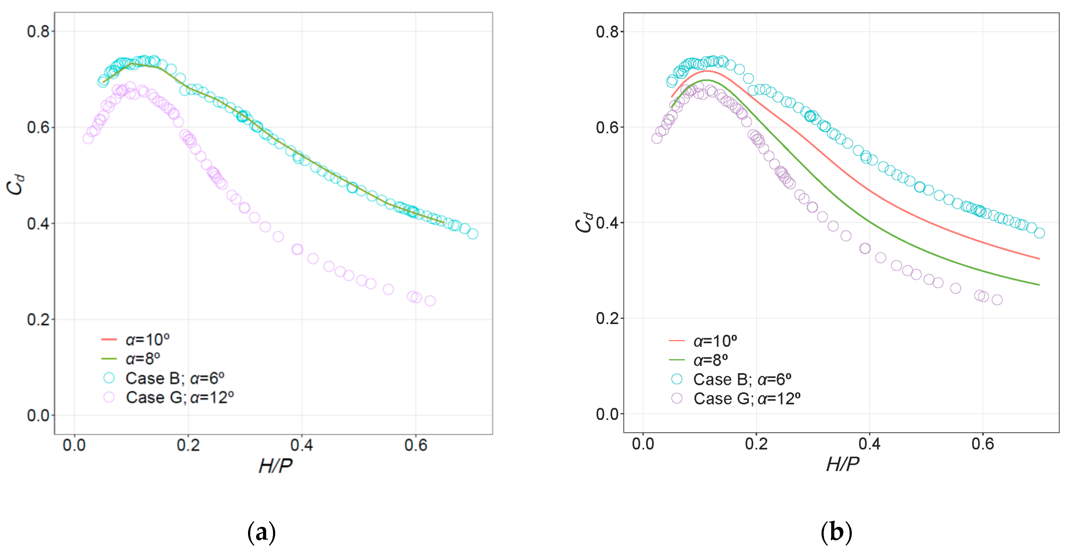
The previous models A–J were used to estimate the values of Cd for intermediate configurations between those analyzed in the laboratory. The intermediate cases are identical geometrically except for the new α values of 8° and 10°. Without experimental Cd values for these intermediate configurations, a direct evaluation is not possible. However, the data are well behaved and interpolated results can be critiqued based on observed trends and neighboring data. Figure 7 shows the results obtained with the NN and RF models when Cases B and G were taken as reference. As in the previous case, similar graphs for other intermediate cases are included in Figures S5 and S6 (Supplementary Materials).
3.3. Model Interpretation
3.3.1. Variable Importance
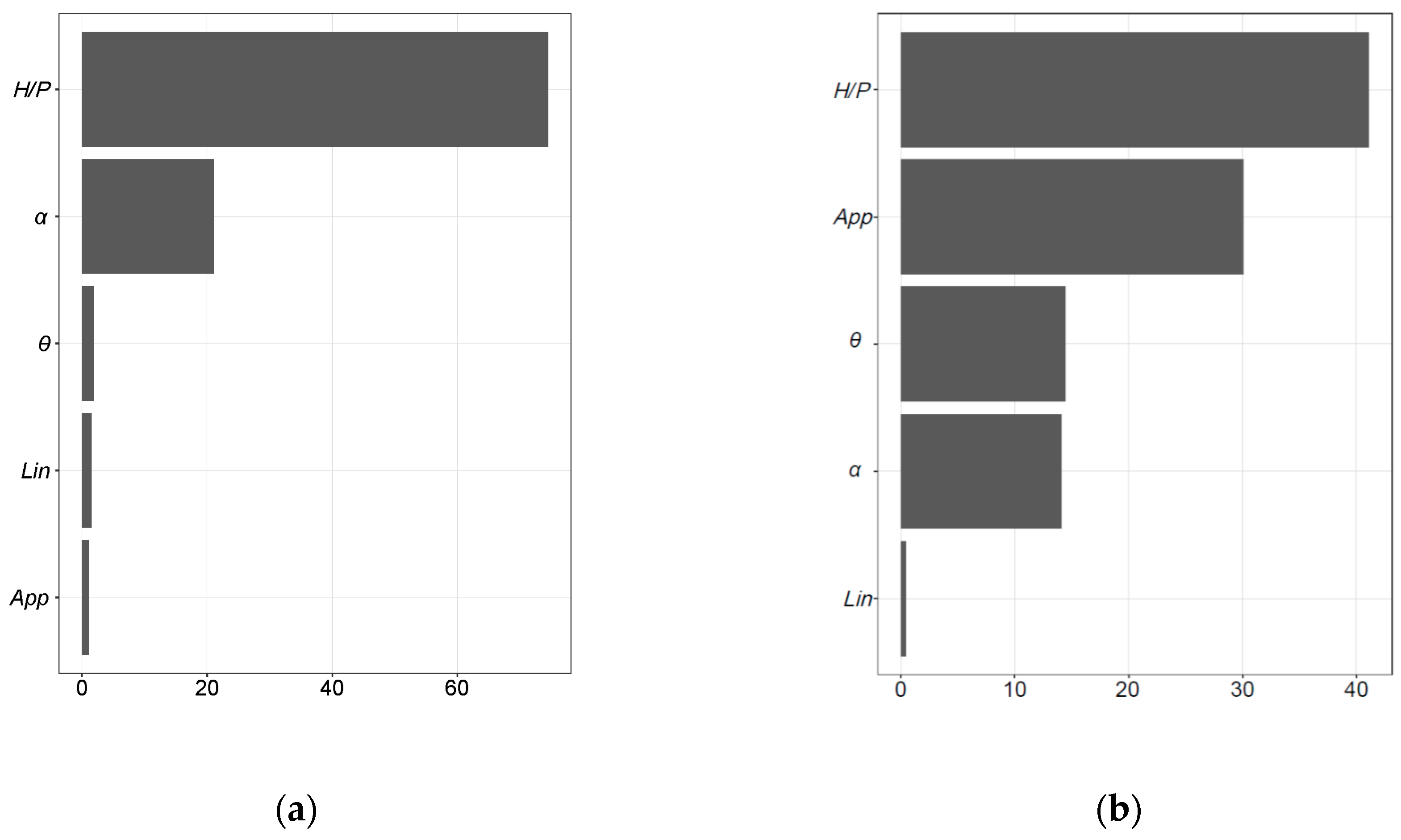
One valuable aspect of ML algorithms is the potential identification of dominant or most influential parameters and parameter relationships. This insight typically complements experimental or field observations; therefore, this study used the RF and NN algorithms to estimate geometric variables’ level of influence when estimating discharge. As illustrated in Figure 8, the dominant parameter for the RF algorithm was H/P, followed by α. This confirms experimental observations and is also in part a function of the experimental dataset used herein. With regard to NN, H/P was also influential but additional importance was also placed on the weir configuration (approach).
3.3.2. Partial Dependence Plots
The average effect of the two most influential variables for RF and NN models is plotted in Figure 9. Both models capture the main effect of H/P on Cd, with small differences. The partial dependence on α is almost identical between both models.
3.4. Non-Tested Geometries
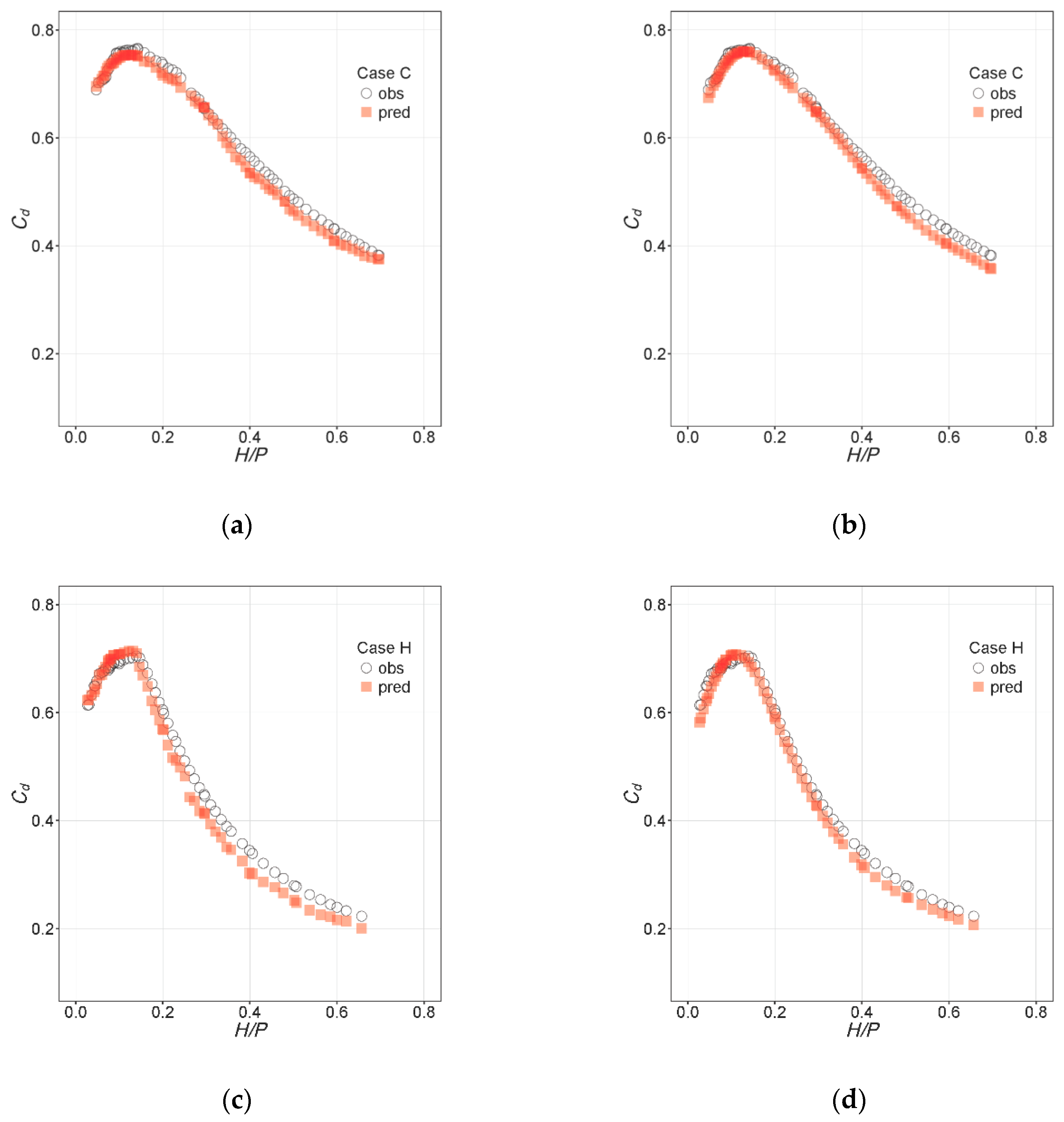
The same training procedure was followed to fit two separate models after removing Cases C and H from the training set. The Cd values for these configurations were then computed and results were compared to experimental Cd values. The results are shown in Figure 10 with accuracy indexes provided in Table 5.
4. Discussion
4.1. Unique Expression
A unique function for the estimation of Cd was possible for both algorithms based on the geometric information and H/P. Due to the nature of the algorithms, this function does not have a simple expression. It does represent a univocal mapping between the input variables (geometric and hydraulic load) and the discharge coefficient. In both cases, the accuracy of the estimation for the configurations tested in the laboratory is of the same order of magnitude as that of the Cd measurements. Therefore, they can be used to obtain the response of the system under these conditions with a simple process of parameter tuning. This is an advantage over other conventional curve-fitting methods such as polynomials, for which the terms of the interpolating polynomial need to be defined a priori; the final expression is typically the result of a trial-and-error process and often involves complex terms (e.g., Reference [54]). Additional verifications are also unnecessary when using a well-trained algorithm, such as using separated expressions for different values of H/P (e.g., Reference [21]).
4.2. Interpolation
When the models were applied to estimate Cd for untested geometric configurations, it was observed that the RF models are incapable of interpolating between two configurations that differ in one critical geometric parameter such as α. In Figure 7, it can be observed that the predictions of the RF model for intermediate α (i.e., 8° and 10°) between Cases B and G are equal to those obtained for case G, with α = 12°. This outcome is rooted in the nature of the algorithm. It is based on trees, which in turn generate a prediction by dividing the space of inputs in disjoint regions and assigning a prediction equal to the mean value of the observations in that region. When dealing with α, the algorithm identifies a point of division of the range in α = 6°. Since α only takes values of 6° and 12° in the training set, the resulting model applies the same learned effect of α for all values greater than 6. It was verified that, indeed, the prediction is the same for other values of α > 6°.
These results are due to the small number of predictor variables and with a somewhat limited dataset of only two α values within the training cases. In fact, α could be considered categorical (α = 6° yes/no), although, in such a case, the algorithm would not allow making predictions for α other than 6° or 12°. This behavior of RF models does not prevent them from being useful for interpolation in other cases, when training data are richer and there is no such difference between the most influential variable (H/P, numerical with values throughout its range) and the rest (categorical or numerical with few values, such as α and θ).
The NN model offers a reasonable estimate of Cd in the intermediate cases. The nature of the algorithm results in a smooth response surface in these conditions and, therefore, the estimates are between the reference cases (Figure 7b). This is a clear advantage of NN over RF in this case of application (i.e., data limitations).
4.3. Model Interpretation
The results for model interpretation are similar for both algorithms in terms of the partial dependence plots. The average effect of H/P on Cd was correctly captured, as well as the increment in Cd for α = 12°, as compared to the homologous cases with α = 6°.
Regarding the variable importance, relevant differences are presented in Figure 8. Although H/P was identified as the most influential or important variable for both models, the order and magnitude of the importance for the remaining variables are clearly different. The following considerations are presented when analyzing these results:
- The nature of each model and the respective procedures for calculating the importance of the variable set are different.
- Some variables were strongly correlated. For example, all cases with Lin = 1 also have θ = 0.
- The random component of each algorithm influences the results.
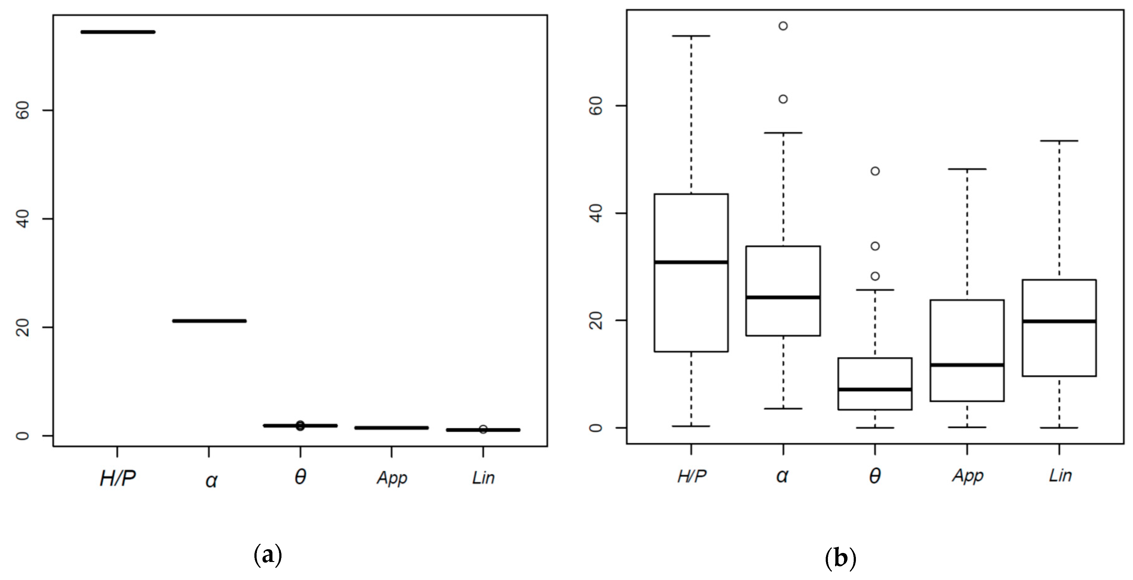
The first two premises imply that the conclusions drawn should be taken with caution. Regarding point 3, to analyze the effect of randomness on predicted results, an additional test was carried out where 100 models were generated from each of the algorithms analyzed, maintaining the training parameters and data, such that the effect of randomness was isolated. The results regarding the importance of the variables are shown in Figure 11 in the form of boxplots. While the importance of the variables in the RF model is practically constant, the NN shows great variation and, thus, results are dependent on the random component of the algorithm. Based on the median of the values obtained, the two most important variables (H/P and α) are in agreement. However, the remaining three variables are relevant for the NN model, which contrasts with the results of the RF model, for which they are almost negligible.
The results of variable importance obtained for the NN model fits better with intuition based on engineering knowledge. In addition, the NN model featured a lower prediction error and the best interpolation, which adds reliability to the results of its interpretation [45]. Nonetheless, the variance of the results needs to be considered in the analysis.
4.4. External Validation
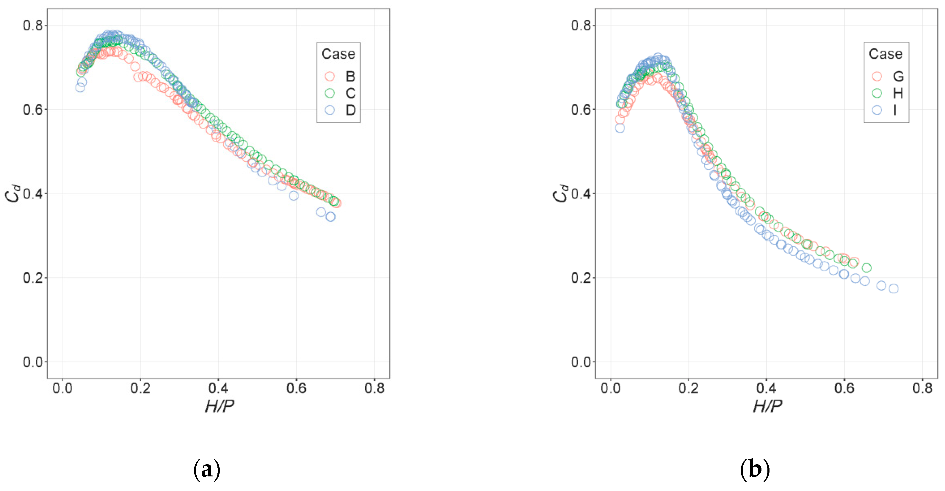
The results obtained when using Cases C and H as external validation are satisfactory in principle, since the resulting accuracy is also similar to that of the Cd measurements. However, these results cannot be extrapolated to the general case, since the Cd values for Cases C and H are similar to the corresponding reference ones: B and D for C and G and I for H. This can be seen in Figure 12.
This is the reason why the predictions of RFs have low error, despite difficulties with interpolation; they are mostly based on those for similar cases.
The metamodels based on NNs can be used to estimate the response for similar configurations to those tested in laboratory, provided appropriate data are available. With the tests used in this work, external validation can only be done for cases with θ = 20°, since the results for θ = 10° and θ = 30° were obtained and available. At least another value of α would be required to perform a similar analysis for that input.
In this sense, the results for interpolation are considered useful to show the possibilities of NN models to enrich a database of experimental results.
5. Summary and Conclusions
Models were presented to estimate the discharge of arced labyrinth spillways based on two machine learning algorithms (random forest and neural network) and experimental data for 10 different geometric configurations. The following conclusions can be drawn regarding this approach from an analysis of the results:
- Both algorithms may obtain a unique mapping that relates discharge to hydraulic head and the geometry of the tested configurations. This is an alternative to other commonly used methods such as curve-fitting experimental data (e.g., polynomials), as it avoids the iterative process of selecting terms and the need to handle complex expressions.
- Although the analysis of these models is more complex, some tools are available to obtain an estimate of the effect of each input variable in the system response, which can be useful for the design of laboratory test campaigns. This is particularly applicable for arced labyrinth spillways where there are many parameters and limited published information.
- The NN models offered reasonable predictions of the discharge curves for intermediate configurations between those tested in the laboratory. Although their precision cannot be quantified because experimental results are not available for intermediate configurations, the results suggest that they can be used to reduce the number of configurations to be tested experimentally in certain settings. These results also follow similar observed trends for linear labyrinth weirs located in a channel [8].
- For those same intermediate cases, the RF model estimation was incorrect; variation along numeric variables for which little training data are available (e.g., α in the case study) occurs in steps. A more diverse dataset would be required to obtain a good interpolation with an RF model in this instance.
- The results of the NN models can vary significantly due to the random component of the initialization of the weights at the beginning of the training. Thus, an appropriate training is critical to obtain valid results.
In the analysis of the discharge capacity of hydraulic structures such as arced labyrinth weirs, ML techniques can provide insights regarding input parameters and can be an effective alternative to curve fitting to obtain a continuous function that approximates the experimental results. This can be achieved with the RF and NN algorithms considered herein and with little preparation effort.
In addition, both algorithms can also be used to obtain an estimate of the weir discharge coefficient for configurations not tested in the laboratory. In this case, however, the goodness of the estimates will depend on the variety of data available, i.e., the diversity of the configurations tested.
If a diverse set of experimental results is available, the analysis of the ML models enables evaluation of the effect of geometric and hydraulic properties (e.g., arc configuration, total head) on discharge capacity, which in turn can be a useful element in design optimization processes.
Supplementary Materials
The following are available online at https://www.mdpi.com/2073-4441/11/3/544/s1: Table S1: Conversion of categorical variables into numeric for the NN model; Figure S1: Effect of mtry on prediction accuracy for RF models. Results for 5 repetitions of each mtry value; Figure S2: Parameter tuning for NN models based on repeated cross-validation; Figure S3: Estimated discharge curves with RF model. Observations (gray) vs. predictions (red) for Cases B, C, D, F, G, H, I, and J; Figure S4: Estimated discharge curves with NN model. Observations (gray) vs. predictions (red) for Cases B, C, D, F, G, H, I, and J; Figure S5: Estimated discharge curves with RF model for intermediate cases. Reference cases (gray) and predictions for α = 8° and α = 10°: (a) between Case A and Case F; (b) between Case C and Case H; (c) between Case D and Case I; (d) between Case E and Case J. Note that the predictions are identical for α = 8°, 10°, and 12°; Figure S6: Estimated discharge curves with NN model for intermediate cases. Reference cases (gray) and predictions for α = 8° and α = 10°: (a) between Case A and Case F; (b) between Case C and Case H; (c) between Case D and Case I; (d) between Case E and Case J.
Author Contributions
Conceptualization, Data curation, formal analysis, funding acquisition, investigation, methodology, project administration, and resources, F.S. and B.M.C.; software, F.S.; supervision, F.S. and B.M.C.; validation, B.M.C.; visualization, writing—original draft, writing—review and editing, F.S. and B.M.C.
Funding
This research was partially funded by the State of Utah through the Utah Water Research Laboratory, as well as by the Generalitat de Catalunya through the CERCA Program and by the Spanish Ministry of Science, Innovation, and Universities through the project COFRE (RTC-2017-6417-5).
Conflicts of Interest
The authors declare no conflict of interest.
References
- Purvis, K. Where Are the World’s Most Water-Stressed Cities? The Guardian. 2016. Available online: https://www.theguardian.com/cities/2016/jul/29/where-world-most-water-stressed-cities-drought (accessed on 15 March 2019).
- Conner, R. The United Nations World Water Development Report 2015: Water for a Sustainable World; United Nations Educational, Scientific and Cultural Organization: Paris, France, 2015. [Google Scholar]
- Crookston, B.M.; Paxson, G.S.; Campbell, D.B. Effective spillways: Harmonizing labyrinth weir hydraulic efficiency and project requirements. In Labyrinth and Piano Key Weirs II—PKW 2013; Erpicum, S., Laugier, F., Pfister, M., Pirotton, M., Cicéro, G.-M., Schleiss, A., Eds.; CRC Press: London, UK, 2013. [Google Scholar]
- Gentilini, B. Stramazzi con cresta a planta obliqua e a zig-zag. In Memorie e Studi dell Instituto di Idraulica e Construzioni Idrauliche del Regil Politecnico di Milano, No. 48; Politecnico di Milano: Milano, Italy, 1941. (In Italian) [Google Scholar]
- Taylor, G. The Performance of Labyrinth Weirs. Ph.D. Thesis, University of Nottingham, Nottingham, UK, 1968. [Google Scholar]
- Magalhães, A.; Lorena, M. Hydraulic Design of Labyrinth Weirs; Report No. 736; National Laboratory of Civil Engineering: Lisbon, Portugal, 1989. [Google Scholar]
- Tullis, P.; Amanian, N.; Waldron, D. Design of labyrinth weir spillways. J. Hydraul. Eng. 1995, 121, 247–255. [Google Scholar] [CrossRef]
- Crookston, B.M. Labyrinth Weirs. Ph.D. Thesis, Utah State University, Logan, UT, USA, 2010. [Google Scholar]
- Labyrinth and Piano Key Weirs; Erpicum, S.; Laugier, F.; Boillat, J.-L.; Pirotton, M.; Reverchon, B.; Schleiss, A.J. (Eds.) CRC Press: Boca Raton, FL, USA, 2011. [Google Scholar]
- Labyrinth and Piano Key Weirs II—PKW 2013; Erpicum, S.; Laugier, F.; Pfister, M.; Pirotton, M.; Cicero, G.-M.; Schleiss, A. (Eds.) CRC Press: London, UK, 2013. [Google Scholar]
- San Mauro, J.; Salazar, F.; Toledo, M.A.; Caballero, F.J.; Ponce-Farfan, C.; Ramos, T. Physical and numerical modeling of labyrinth weirs with polyhedral bottom. Ing. Agua 2016, 20, 127–138. [Google Scholar] [CrossRef]
- Erpicum, S.; Tullis, B.P.; Lodomez, M.; Archambeau, P.; Dwals, B.; Pirotton, M. Scale effects in physical piano key weir models. J. Hydraul. Res. 2016, 54, 692–698. [Google Scholar] [CrossRef]
- Pfister, M.; Battisacco, E.; De Cesare, G.; Schleiss, A.J. Scale effects related to the rate curve of cylindrically crested Piano Key weirs. In Labyrinth and Piano Key Weirs II—PKW 2013; CRC Press/Balkema: Leiden, The Netherlands, 2013. [Google Scholar]
- Lopes, R.; Matos, J.; Melo, J. Discharge capacity and residual energy of labyrinth weirs. In International Junior Researcher and Engineer Workshop on Hydraulic Structures (IJREWHS ‘06); Montemor-o-Novo, Hydraulic Model Report No. CH61/06; Div. of Civil Engineering, The University of Queensland: Brisbane, Australia, 2006; pp. 47–55. [Google Scholar]
- Lopes, R.; Matos, J.; Melo, J. Characteristic depths and energy dissipation downstream of a labyrinth weir. In International Junior Researcher and Engineer Workshop on Hydraulic Structures (IJREWHS ‘08); PLUS-Pisa University Press: Pisa, Italy, 2018. [Google Scholar]
- Pfister, M.; Capobianco, D.; Tullis, B.; Schleiss, A. Debris-blocking sensitivity of piano key weirs under reservoir-type approach flow. J. Hydraul. Eng. 2013, 139, 1134–1141. [Google Scholar] [CrossRef]
- Crookston, B.M.; Mortensen, D.; Stanard, T.; Tullis, B.P.; Vasquez, V. Debris and maintenance of labyrinth spillways. In Proceedings of the 35th Annual USSD Conference, Louisville, KY, USA, 13–17 April 2015; [CD-ROM]. USSD: Westminster, CO, USA, 2015. [Google Scholar]
- Darvas, L. Discussion of performance and design of labyrinth weirs, by Hay and Taylor. J. Hydraul. Eng. 1971, 97, 1246–1251. [Google Scholar]
- Yildiz, D.; Uzecek, E. Modeling the performance of labyrinth spillways. Hydropower 1996, 3, 71–76. [Google Scholar]
- Page, D.; García, V.; Ninot, C. Aliviaderos en laberinto. presa de María Cristina. Ing. Civil 2007, 146, 5–20. (In Spanish) [Google Scholar]
- Crookston, B.M.; Tullis, B.P. Arced labyrinth weirs. J. Hydraul. Eng. 2012, 138, 555–562. [Google Scholar] [CrossRef]
- Crookston, B.M.; Tullis, B.P. Discharge efficiency of reservoir-application-specific labyrinth weirs. J. Irrig. Drain. Eng. 2012, 138, 564–568. [Google Scholar] [CrossRef]
- Christensen, N.A. Flow Characteristics of Arced Labyrinth Weirs. Master’s Thesis, Utah State University, Logan, UT, USA, 2012. [Google Scholar]
- Thompson, E.; Cox, N.; Ebner, L.; Tullis, B. The hydraulic design of an arced labyrinth weir at Isabella Dam. In Hydraulic Structures and Water System Management, Proceedings of the 6th IAHR International Symposium on Hydraulic Structures, Portland, OR, USA, 27–30 June 2016; Crookston, B., Tullis, B., Eds.; Utah State University: Logan, UT, USA, 2016; pp. 230–239. ISBN 978-1-884575-75-4. [Google Scholar] [CrossRef]
- Cremona, C.; Santos, J. Structural health monitoring as a big-data problem. Struct. Eng. Int. 2018, 28, 243–254. [Google Scholar] [CrossRef]
- Dawson, C.W.; Wilby, R.L. Hydrological modelling using artificial neural networks. Prog. Phys. Geogr. 2001, 25, 80–108. [Google Scholar] [CrossRef]
- ASCE Task Committee on Application of Artificial Neural Networks in Hydrology. Artificial neural networks in hydrology. I: Preliminary concepts. J. Hydrol. Eng. 2000, 5, 115–123. [Google Scholar] [CrossRef]
- ASCE Task Committee on Application of Artificial Neural Networks in Hydrology. Artificial neural networks in hydrology. II: Hydrologic applications. J. Hydrol. Eng. 2000, 5, 124–137. [Google Scholar] [CrossRef]
- de Granrut, M.; Simon, A.; Dias, D. Artificial neural networks for the interpretation of piezometric levels at the rock-concrete interface of arch dams. Eng. Struct. 2019, 178, 616–634. [Google Scholar] [CrossRef]
- Mata, J.; Leitão, N.S.; De Castro, A.T.; Da Costa, J.S. Construction of decision rules for early detection of a developing concrete arch dam failure scenario. A discriminant approach. Comput. Struct. 2014, 142, 45–53. [Google Scholar] [CrossRef]
- Salazar, F.; Toledo, M.A.; Oñate, E.; Morán, R. An empirical comparison of machine learning techniques for dam behaviour modelling. Struct. Saf. 2015, 56, 9–17. [Google Scholar] [CrossRef] [Green Version]
- Salazar, F.; Toledo, M.Á.; Oñate, E.; Suárez, B. Interpretation of dam deformation and leakage with boosted regression trees. Eng. Struct. 2016, 119, 230–251. [Google Scholar] [CrossRef]
- Salazar, F.; Toledo, M.Á.; González, J.M.; Oñate, E. Early detection of anomalies in dam performance: A methodology based on boosted regression trees. Struct. Control Health Monit. 2017, 24. [Google Scholar] [CrossRef]
- Herrera, M.; Torgo, L.; Izquierdo, J.; Pérez-García, R. Predictive models for forecasting hourly urban water demand. J. Hydrol. 2010, 387, 141–150. [Google Scholar] [CrossRef]
- Valero, D.; Bung, D.B. Artificial Neural Networks and pattern recognition for air-water flow velocity estimation using a single-tip optical fibre probe. J. Hydro-Environ. Res. 2018, 19, 150–159. [Google Scholar] [CrossRef]
- Bashiri Atrabi, H.; Dewals, B.; Pirotton, M.; Archambeau, P.; Erpicum, S. Towards a new design equation for piano key weirs discharge capacity. In Proceedings of the 6th International Symposium on Hydraulic Structures, Portland, OR, USA, 27–30 June 2016. [Google Scholar]
- Emiroglu, M.E.; Kisi, O. Prediction of discharge coefficient for trapezoidal labyrinth side weir using a neuro-fuzzy approach. Water Resour. Manag. 2013, 27, 1473–1488. [Google Scholar] [CrossRef]
- Azamathulla, H.M.; Haghiabi, A.H.; Parsaie, A. Prediction of side weir discharge coefficient by support vector machine technique. Water Sci. Technol. Water Supply 2016, 16, 1002–1016. [Google Scholar] [CrossRef]
- Salazar, F.; Morán, R.; Rossi, R.; Oñate, E. Analysis of the discharge capacity of ra-dial-gated spillways using CFD and ANN—Oliana Dam case study. J. Hydraul. Res. 2013, 51, 244–252. [Google Scholar] [CrossRef]
- Mata, J. Interpretation of concrete dam behaviour with artificial neural network and multiple linear regression models. Eng. Struct. 2011, 33, 903–910. [Google Scholar] [CrossRef]
- Salazar, F.; Morán, R.; Toledo, M.Á.; Oñate, E. Data-based models for the prediction of dam behaviour: A review and some methodological considerations. Arch. Comput. Methods Eng. 2017, 24, 1–21. [Google Scholar] [CrossRef]
- Díaz-Uriarte, R.; De Andres, S.A. Gene selection and classification of microarray data using random forest. BMC Bioinform. 2006, 7. [Google Scholar] [CrossRef] [PubMed]
- Tullis, B.; Young, N.; Crookston, B. Size-scale effects of labyrinth weir hydraulics. In Proceedings of the 7th IAHR International Symposium on Hydraulic Structures, Aachen, Germany, 15–18 May 2018. [Google Scholar] [CrossRef]
- R Core Team. R: A Language and Environment for Statistical Computing; R Foundation for Statistical Computing: Vienna, Austria; Available online: https://www.R-project.org/ (accessed on 15 March 2019).
- Breiman, L. Statistical modeling: The two cultures (with comments and a rejoinder by the author). Stat. Sci. 2001, 16, 199–231. [Google Scholar] [CrossRef]
- Ishwaran, H.; Kogalur, U.B. Random survival forests for R. R News 2008, 7, 25–31. [Google Scholar] [CrossRef]
- Liaw, A.; Wiener, M. Classification and regression by randomForest. R News 2002, 2, 18–22. [Google Scholar]
- Venables, W.N.; Ripley, B.D. Modern Applied Statistics with S, 4th ed.; Springer: New York, NY, USA, 2002; ISBN 0-387-95457-0. [Google Scholar]
- Bishop, C.M. Neural Networks for Pattern Recognition; Oxford University Press: New York, NY, USA, 1995. [Google Scholar]
- Kuhn, M. Caret package. J. Stat. Softw. 2008, 28, 1–26. [Google Scholar]
- Olden, J.D.; Jackson, D.A. Illuminating the “black box”: A randomization approach for understanding variable contributions in artificial neural networks. Ecol. Model. 2002, 154, 135–150. [Google Scholar] [CrossRef]
- Beck, M. NeuralNetTools: Visualization and analysis tools for neural networks. J. Stat. Softw. 2018, 85, 1–20. [Google Scholar] [CrossRef] [PubMed]
- Greenwell, B.M. pdp: An R package for constructing partial dependence plots. R J. 2017, 9, 421–436. [Google Scholar] [CrossRef]
- Machiels, O.; Pirotton, M.; Pierre, A.; Dewals, B.; Erpicum, S. Experimental parametric study and design of Piano Key Weirs. J. Hydraul. Res. 2014, 52, 326–335. [Google Scholar] [CrossRef]
Figure 1.
Examples of arced labyrinth weirs: (a) Maguga Spillway in Swaziland during construction, and (b) the physical model of Isabella Spillway to be built in California, United States of America (USA). Photos courtesy of D. van Wyk (a) and B. Tullis (b).
Figure 1.
Examples of arced labyrinth weirs: (a) Maguga Spillway in Swaziland during construction, and (b) the physical model of Isabella Spillway to be built in California, United States of America (USA). Photos courtesy of D. van Wyk (a) and B. Tullis (b).

Figure 2.
Arced labyrinth spillway as proposed by Crookston [8].
Figure 2.
Arced labyrinth spillway as proposed by Crookston [8].

Figure 3.
Tested labyrinth spillway orientation in a reservoir: (a) linear projecting, (b) arced projecting, and (c) linear flush.
Figure 3.
Tested labyrinth spillway orientation in a reservoir: (a) linear projecting, (b) arced projecting, and (c) linear flush.

Figure 4.
Experimental data recorded by Crookston [8] for (a) α = 12° and (b) α = 6° labyrinth weir configurations.
Figure 4.
Experimental data recorded by Crookston [8] for (a) α = 12° and (b) α = 6° labyrinth weir configurations.

Figure 5.
Cd observations vs. predictions of the (a) random forest (RF) model, and (b) neural network (NN) model using the validation set.
Figure 5.
Cd observations vs. predictions of the (a) random forest (RF) model, and (b) neural network (NN) model using the validation set.

Figure 6.
Discharge curves. Observations (circles) vs. predictions (squares) for (a) Case A, RF; (b) Case A, NN; (c) Case E, RF; and (d) Case E, NN.
Figure 6.
Discharge curves. Observations (circles) vs. predictions (squares) for (a) Case A, RF; (b) Case A, NN; (c) Case E, RF; and (d) Case E, NN.


Figure 7.
Discharge curves for intermediate cases between B and G. Reference cases (hollow circles) and predictions for α = 8° and α = 10°: (a) RF; (b) NN. Note that the predictions from RF are identical for α = 8°, 10°, and 12°.
Figure 7.
Discharge curves for intermediate cases between B and G. Reference cases (hollow circles) and predictions for α = 8° and α = 10°: (a) RF; (b) NN. Note that the predictions from RF are identical for α = 8°, 10°, and 12°.

Figure 8.
Input variable importance for (a) RF model, and (b) NN model.

Figure 9.
Partial dependence of Cd on (a) H/P, and on (b) α, as learned by the models.

Figure 10.
Predictions vs. observations for Cases C and H with new models trained using Cases A, B, D–G, I, and J: (a) Case C, RF; (b) Case C, NN; (c) Case H, RF; (d) Case H, NN.
Figure 10.
Predictions vs. observations for Cases C and H with new models trained using Cases A, B, D–G, I, and J: (a) Case C, RF; (b) Case C, NN; (c) Case H, RF; (d) Case H, NN.

Figure 11.
Normalized variable importance for 100 replications of (a) the RF model, and (b) the NN model.
Figure 11.
Normalized variable importance for 100 replications of (a) the RF model, and (b) the NN model.

Figure 12.
Experimental values for Cd in the cases used as external validation: (a) Case C and (b) Case H, as compared to those with similar values of α.
Figure 12.
Experimental values for Cd in the cases used as external validation: (a) Case C and (b) Case H, as compared to those with similar values of α.


Table 1.
Physical model test matrix.
| Case | α (°) | θ (°) | Number of Cycles | Reservoir Orientation |
|---|---|---|---|---|
| A | 12 | 0 | 5 | Linear, projecting |
| B | 12 | 10 | 5 | Arced, projecting |
| C | 12 | 20 | 5 | Arced, projecting |
| D | 12 | 30 | 5 | Arced, projecting |
| E | 12 | 0 | 5 | Linear, flush |
| F | 6 | 0 | 5 | Linear, projecting |
| G | 6 | 10 | 5 | Arced, projecting |
| H | 6 | 20 | 5 | Arced, projecting |
| I | 6 | 30 | 5 | Arced, projecting |
| J | 6 | 0 | 5 | Linear, flush |
Table 2.
Input variables considered.
| Variable | Code | Values | Units |
|---|---|---|---|
| Head over crest | H/P | 0–0.75 | - |
| Cycle sidewall angle | α | 6°, 12° | (°) |
| Cycle arc angle | θ | 0°, 10°, 20°, 30° | (°) |
| Linearity | Lin | Linear, non-linear | - |
| Approach configuration | App | Flush, projecting, arc projecting | - |
Table 3.
Example of conversion of categorical variables into numerical values. Table S1 (Supplementary Materials) includes the complete list of configurations and new variables added.
Table 3.
Example of conversion of categorical variables into numerical values. Table S1 (Supplementary Materials) includes the complete list of configurations and new variables added.
| Case | Original Variable | New Variables | ||
|---|---|---|---|---|
| Configuration | Arc Projecting | Flushed | Projecting | |
| E | Flushed | 0 | 1 | 0 |
| F | Projecting | 0 | 0 | 1 |
| G | Arc Projecting | 1 | 0 | 0 |
Table 4.
Prediction accuracy of both models for the training set.
| Algorithm | Dataset | ME 1 | RMSE 2 | MAE 3 | MAPE 4 |
|---|---|---|---|---|---|
| Random forest | Training | 0.001 | 0.008 | 0.006 | 1.258 |
| Validation | 0.000 | 0.008 | 0.006 | 1.382 | |
| Neural networks | Training | 0.000 | 0.008 | 0.006 | 1.147 |
| Validation | 0.000 | 0.008 | 0.006 | 1.255 |
1 ME = mean error; 2 RMSE = root-mean-squared error; 3 MAE = mean absolute error; 4 MAPE = mean absolute percentage error.
Table 5.
Prediction accuracy of random forest (RF) and neural networks (NN) for Cases C and H, once removed from the training set.
Table 5.
Prediction accuracy of random forest (RF) and neural networks (NN) for Cases C and H, once removed from the training set.
| Algorithm | Case | RMSE | MAPE |
|---|---|---|---|
| Random forest | C | 0.016 | 2.500 |
| H | 0.027 | 5.625 | |
| Neural networks | C | 0.018 | 2.947 |
| H | 0.018 | 3.883 |
© 2019 by the authors. Licensee MDPI, Basel, Switzerland. This article is an open access article distributed under the terms and conditions of the Creative Commons Attribution (CC BY) license (http://creativecommons.org/licenses/by/4.0/).
Share and Cite
MDPI and ACS Style
Salazar, F.; Crookston, B.M. A Performance Comparison of Machine Learning Algorithms for Arced Labyrinth Spillways. Water 2019, 11, 544. https://doi.org/10.3390/w11030544
AMA Style
Salazar F, Crookston BM. A Performance Comparison of Machine Learning Algorithms for Arced Labyrinth Spillways. Water. 2019; 11(3):544. https://doi.org/10.3390/w11030544
Chicago/Turabian StyleSalazar, Fernando, and Brian M. Crookston. 2019. "A Performance Comparison of Machine Learning Algorithms for Arced Labyrinth Spillways" Water 11, no. 3: 544. https://doi.org/10.3390/w11030544
Note that from the first issue of 2016, this journal uses article numbers instead of page numbers. See further details here.