Article

Comparative Analysis of High-Resolution Soil Moisture Simulations from the Soil, Vegetation, and Snow (SVS) Land Surface Model Using SAR Imagery Over Bare Soil

1
Science and Technology Branch, Environment and Climate Change Canada, Dorval, QC H9P 1J3, Canada
2
Science and Technology Branch, Agriculture and Agri-Food Canada, Winnipeg, MB R3C 3G7, Canada
3
Science and Technology Branch, Agriculture and Agri-Food Canada, Ottawa, ON K1A 0C6, Canada
*
Author to whom correspondence should be addressed.
Water 2019, 11(3), 542; https://doi.org/10.3390/w11030542
Submission received: 28 December 2018 / Revised: 27 February 2019 / Accepted: 12 March 2019 / Published: 15 March 2019
(This article belongs to the Section Hydrology)

Abstract

:
Soil moisture is a key variable in Earth systems, controlling the exchange of water and energy between land and atmosphere. Thus, understanding its spatiotemporal distribution and variability is important. Environment and Climate Change Canada (ECCC) has developed a new land surface parameterization, named the Soil, Vegetation, and Snow (SVS) scheme. The SVS land surface scheme features sophisticated parameterizations of hydrological processes, including water transport through the soil. It has been shown to provide more accurate simulations of the temporal and spatial distribution of soil moisture compared to the current operational land surface scheme. Simulation of high resolution soil moisture at the field scale remains a challenge. In this study, we simulate soil moisture maps at a spatial resolution of 100 m using the SVS land surface scheme over an experimental site located in Manitoba, Canada. Hourly high resolution soil moisture maps were produced between May and November 2015. Simulated soil moisture values were compared with estimated soil moisture values using a hybrid retrieval algorithm developed at Agriculture and Agri-Food Canada (AAFC) for soil moisture estimation using RADARSAT-2 Synthetic Aperture Radar (SAR) imagery. Statistical analysis of the results showed an overall promising performance of the SVS land surface scheme in simulating soil moisture values at high resolution scale. Investigation of the SVS output was conducted both independently of the soil texture, and as a function of the soil texture. The SVS model tends to perform slightly better over coarser textured soils (sandy loam, fine sand) than finer textured soils (clays). Correlation values of the simulated SVS soil moisture and the retrieved SAR soil moisture lie between 0.753–0.860 over sand and 0.676-0.865 over clay, with goodness of fit values between 0.567–0.739 and 0.457–0.748, respectively. The Root Mean Square Difference (RMSD) values range between 0.058–0.062 over sand and 0.055–0.113 over clay, with a maximum absolute bias of 0.049 and 0.094 over sand and clay, respectively. The unbiased RMSD values lie between 0.038–0.057 over sand and 0.039–0.064 over clay. Furthermore, results show an Index of Agreement (IA) between the simulated and the derived soil moisture always higher than 0.90.

1. Introduction

Soil moisture is a key state variable in earth system dynamics. Its spatial distribution and temporal variation play an important role in hydrologic, ecologic, and climatic models in both regional and global scales [1]. At the earth surface, soil moisture is a major component of the water balance, influencing the energy balance in terms of sensible and latent heat fluxes, which act to modify the local boundary level and storm development [2,3,4,5,6,7]. Also, soil moisture influences agricultural productivity, lateral water movement on or below the surface owing to runoff generation, and flood or drought development [7,8,9,10,11,12]. Furthermore, soil moisture is an important parameter for producing accurate meteorological and environmental forecasts, given its interaction with atmospheric variables [13]. The accurate estimation of soil moisture using remotely sensed data [14] or simulations using land surface models [13,15] is necessary at both high and low spatial resolutions.
Volumetric soil moisture can be simulated at the regional and global scale using land surface models driven with atmospheric forcing fields. Weather and climate prediction systems depend on land surface models to provide their surface conditions [16]. Furthermore, land surface models are integral components of environmental prediction and data assimilation systems. In such systems, simulated soil moisture data using land surface models and estimated soil moisture data using remote sensing observations are combined in an assimilation procedure. The Canadian Land Data Assimilation System (CaLDAS) is an environmental prediction and assimilation system developed at Environment and Climate Change Canada (ECCC). CaLDAS provides an accurate estimate of the current state of the land surface and provides initial conditions for the High Resolution Deterministic Prediction System (HRDPS) at ECCC [17,18]. The operational version of CaLDAS is based on a land surface scheme named the Interactions between Soil, Biosphere, and Atmosphere (ISBA) [19,20]. The ISBA land surface model has been used operationally at ECCC since 2001 [21,22].
Recently, an advanced land surface model named the Soil, Vegetation, and Snow (SVS) scheme has been developed at ECCC and is expected to replace ISBA for operational predictions in the near future. SVS is an improved version of the ISBA land surface scheme [15,23]. It is characterized by sophisticated parameterization of the hydrological processes and representation of the water transport through the soil, allowing more accurate simulation of temporal and spatial distribution of soil moisture. The hydrology scheme in SVS introduces increased vertical resolution within the soil column with multiple soil layers, along with vertical water diffusion in the soil based on the Richards equation [24]. It also includes improved parameterizations for surface runoff, lateral flow, and drainage using the information on sub-grid-scale slope and drainage density [15].
A first evaluation of the performance of the SVS model in simulating soil moisture at high resolution was presented in [25]. In that study, soil moisture was simulated over an experimental site in Manitoba, Canada, using the SVS model for the entire summer of 2014 and the simulation results were compared with in situ soil moisture observations. A good agreement between the simulated and observed soil moisture was reported. However, a visual interpretation of the results showed that the modeled soil moisture spatial variability was much weaker than the observed [25]. In another study [13], the performance of an updated version of the SVS model using in situ soil moisture observations was evaluated in a study area which was located within our current experimental site. In that study, the effect of the assumption of homogeneous soil texture versus spatially varying soil texture on the performance of the SVS model was assessed. Results showed that spatially varying soil texture is necessary for improved soil moisture simulation results. The performance of the SVS model for the simulation of soil moisture was also verified in [26] against a set of ground in situ observations of soil moisture over a period of 5 years. Comparison of soil moisture simulations using the SVS model with retrieved soil moisture products from satellite remote sensing imagery has not been done yet, though such a comparison would present the level of agreement between modeled and remotely sensed data, as shown in [27,28].
The innovative aspect of the present study lies in the fact that it provides the first comparison analysis between simulated soil moisture values from the SVS land surface model at high spatial resolution and soil moisture estimated from Synthetic Aperture Radar (SAR) imagery. In this comparative analysis, we investigate the level of agreement between the simulated and estimated soil moisture with respect to the evolution and the variability in time and space of soil moisture. Thus, the present study is complementary to and expands upon the study by Garnaud et al. [25], though it focuses on the capability of the SVS model to capture the spatial variability of the soil moisture, in contrary to the study by Garnaud et al. [25] which mainly focused on the feasibility of the SVS model to capture the soil moisture evolution over time. An experimental site located southwest of Winnipeg, Manitoba, Canada, was selected for the purpose of our study. The soil moisture was simulated using the SVS model, driven by short-range atmospheric forecasts and making use of high-resolution geophysical fields such as crop type and soil texture information. Over the experimental site, twenty four fully polarimetric RADARSAT-2 SAR images were acquired for four different dates (six images for each date) and these were used to estimate soil moisture based on a physical scattering model [14]. Simulated soil moisture obtained from the SVS model was statistically analyzed against the soil moisture estimated from the SAR imagery.

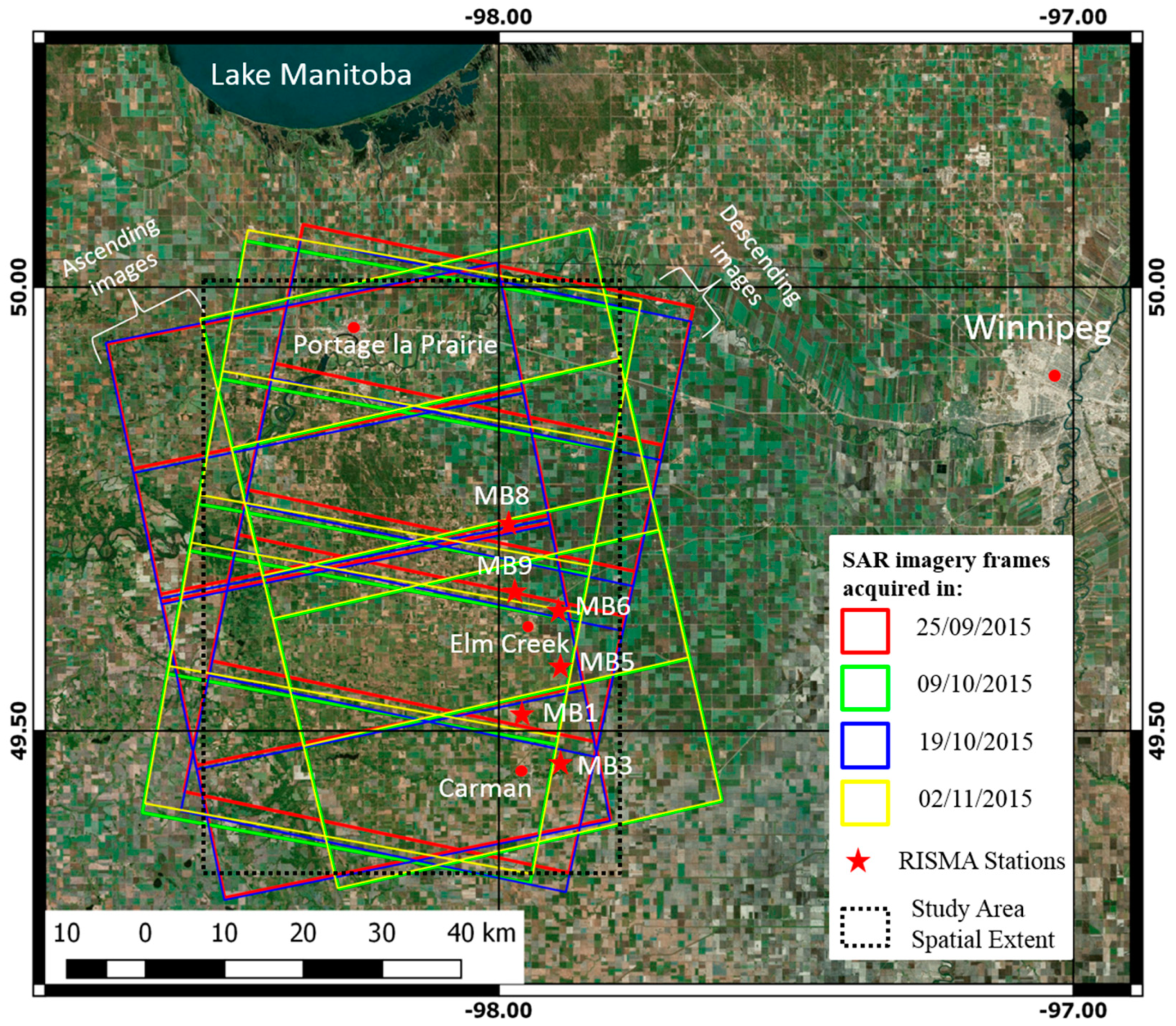
2. Experimental Site and SAR Imagery

A topographically flat experimental site located in southern Manitoba, Canada, close to the city of Winnipeg was selected (Figure 1). The site is a region of intensive agriculture dominated by annual crops which include wheats, soybeans, canola, and corn [29]. In this region of Canada, the growing season takes place between April and September [29]. A map of the land uses for the year of 2015 created by Agriculture and Agri-Food Canada (AAFC) for the experimental site is shown in Figure 2.
Soils in the region have been mapped at a detailed 1:20,000 scale and are available from the Canadian Soil Information Service (CanSIS) website at AAFC (http://sis.agr.gc.ca/cansis/publications/surveys/mb/index.html). Soils in this area were formed from lacustrine depositions from glacial Lake Agassiz [30]. Figure 3 shows soil polygons representing the textural fractions of sand (Figure 3a) and clay (Figure 3b) for the study area. Soil polygons have different sizes depending on the textural fraction in each region. Each polygon has one textural fraction value of sand and clay. Coarser textured sediments (sands) are dominant in the central and western regions of the experimental site while finer textured clay soils occur in the east. The experimental site includes an area of forest cover in the northwest and wetlands in the north and south (Figure 1 and Figure 2), both of which were excluded from our study.
Twenty four Fine Quad Wide (FQW) RADARSAT-2 polarimetric SAR images were acquired in 2015 between September and November during a period of bare soil and sparse vegetation (Figure 1). A summary of the SAR acquisitions is presented in Table 1. Four sets of images were acquired in the September to November period. Each set contains six SAR images; three images in the satellite’s ascending orbit and three images in its descending orbit (Figure 1). SAR incidence angle varies between ascending and descending orbits (Table 1). Ascending (approximately 7 PM local time) and descending (approximately 8 AM local time) image pairs are acquired within 12 h of each other. Rain gauges installed on-site confirmed that no significant precipitation occurred between ascending-descending pairs of acquisitions. Although our study is limited to four dates, the sample size is adequate enough to provide a sufficient assessment of the simulated soil moisture using the SVS model, especially since the experimental site was sufficiently large (75 km × 50 km). It is also worth mentioning that the acquisition of additional SAR imagery was not possible because the period of interest was selected for bare soil in the middle to late fall prior to the arrival of snow. Inspection of the archived weather information confirmed that there was no snowfall during the study period (25 September to 2 November) over the experimental site. In situ soil moisture observations from six Real-time In-situ Soil Monitoring for Agriculture (RISMA) stations were available for the study period (Figure 1).

3. Methodology

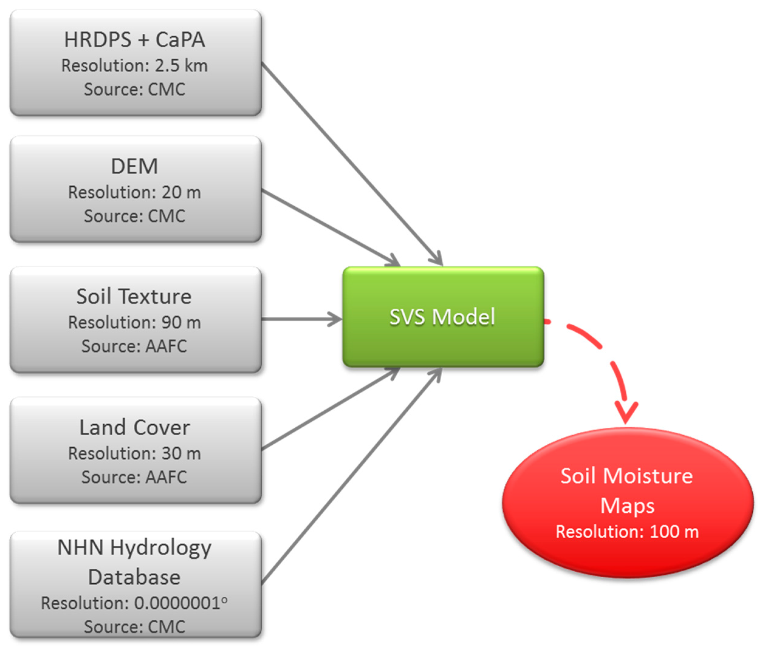
3.1. SVS Experimental Setup

SVS calculates the energy and water budgets for bare ground and vegetation, and two snow packs (over bare ground and low vegetation and under high vegetation), with a new tiling approach [15]. The new tiling approach (Figure 4) divides the land tile for each grid cell into fraction of low vegetation (υl), fraction of high vegetation (υh), and fraction of bare ground (1 − υlυh). The scheme also has improved parameterization of the vegetation thermal coefficient with a new snowpack under vegetation. Furthermore, the SVS model calculates root density functions depending on the vegetation type and multilayer water vertical transport in the soil for each soil layer. New formulas for land surface albedo and emissivity are also included. In SVS, the soil moisture is represented in the soil layers based on vertical transportation, evapotranspiration, and surface and lateral flows [13,15,23]. The evolution of the volumetric water content w within these soil layers (Figure 4) is given by the following differential equation [15]:
w t = F z + S
where F is the water flux between soil layers, z is the soil depth, t is the time, and S is the sink-source terms, including surface evaporation, precipitation, runoff from vegetation, evapotranspiration, surface runoff, lateral flow, snow runoff, base flow, melting, and freezing [15].
The volumetric soil water content for bare ground in the top soil layer w1 can be expressed as:
Δ w 1 Δ t = 1 d 1   [ ( 1 υ l υ h ) ( R r E g ) + ( υ l + υ h ) ( R U υ f 1 , r o o t E t r ) F 2 R U s u r f L f l 1 ]
where d1 is the depth of the top soil layer, Rr is the rainfall rate, Eg is bare soil evaporation, RUυ is the water throughfall from vegetation, Etr is the transpiration scaled based on the root fraction f1,root of the first layer, RUsurf is the surface runoff, Lfl1 is the lateral flow in the first layer, and F2 is the diffusive water flux from the first soil layer to the second. Within the soil column, the vertical discretization consists of N number of soil layers. However, at ECCC 7 soil layers are usually considered when running the SVS with a depth of 5, 10, 20, 40, 100, 200, and 300 cm, respectively. In SVS, the soil surface temperature is calculated with a prognostic equation based on the Force-Restore method [31]. More detailed description of the SVS model physical processes and modeling setup can be found in [15,24]. No further SVS modeling details are provided here for brevity.
A flowchart summarizing the configuration of the SVS model necessary for the soil moisture simulations is shown in Figure 5. In our study, we consider the superficial soil moisture, the top 5 cm, as simulated by SVS. The atmospheric forcing variables needed to drive SVS at 100 m grid spacing are provided by a lower resolution atmospheric model, the High-Resolution Deterministic Prediction System (HRDPS) at 2.5 km grid spacing. The forecast skill of the HRDPS model has been evaluated extensively for both summer and winter in a recent publication [18]. Since the accuracy of the meteorological forcing variables could contribute to differences between soil moisture simulated by the SVS model and soil moisture derived from SAR imagery, we limited the atmospheric forcing variables to short-range (0–6 h) HRDPS forecasts, ensuring that no forcing variables are from forecast ranges beyond 6 h. In [18], it was shown that the HRDPS forecast skill is greater for the shorter forecast ranges which should lead to more accurate simulations of the land-surface, including soil moisture. Eight atmospheric forcing variables are needed to drive SVS, which include precipitation, incident longwave and shortwave radiation, zonal and meridional winds, specific humidity, air temperature and surface pressure. For precipitation, the Canadian Precipitation Analysis (CaPA) [32] methodology is used, which combines a 6 h first-guess precipitation from the HRDPS with precipitation gauge observations from the SYNOP and METAR networks in an optimum interpolation assimilation. The CaPA methodology ensures a high accuracy of precipitation forcing. Owing to the relatively flat experimental site, elevation differences between the low resolution of 2.5 km and the 100 m integration grid were very small and no terrain adaptation of the atmospheric forcing was done.
In addition to the atmospheric forcing provided by HRDPS, additional geophysical field information for the experimental site is necessary to perform the SVS simulations. This includes a Digital Elevation Model (DEM) available at a spatial resolution of 20 m. Furthermore, soil texture information of the test site was obtained from AAFC at a spatial resolution of 90 m along with land cover information at a spatial resolution of 30 m. This product maps general land cover but with the agricultural class further segmented into individual crop types. Running the SVS model also requires hydrological data information provided by the Canadian National Hydrology Network (NHN) database (https://open.canada.ca/data/en/dataset/a4b190fe-e090-4e6d-881e-b87956c07977). This geospatial hydrology database contains geometric information and basic attributes describing Canada’s inland surface waters at a spatial resolution of 0.0000001°.
In our study, the SVS model was run in an open-loop configuration initialized with a “cold start” mode in which the initial conditions were directly derived from the HRDPS output with a resolution of 2.5 km. The model was initialized on 31 May 2015, allowing at least three months before the acquisition of the first RADARSAT-2 image (which was on 25 September) in order to minimize the effects of coarser resolution initial conditions. Also, this ensures that the SVS simulated soil moisture in the top layer has reached the equilibrium condition. Consequently, the simulation of the soil moisture maps started on 31 May 2015 and continued until 2 November 2015 (acquisition date of the last RADARSAT-2 SAR images), with a model time step of 30 min.

3.2. Soil Moisture Retrieval Using SAR Imagery

SAR satellites propagate pulses of microwave energy and the intensity of energy scattered and returned to the satellite is partially dependent upon the amount of water held in the target being illuminated. AAFC has implemented a physical scattering model to estimate surface soil moisture from C-band SAR satellites, including RADARSAT-2, with high accuracy [14]. The algorithm used is the Integral Equation Model (IEM), which is appropriate for random dielectric rough surfaces [33]. AAFC uniquely implemented the IEM in a hybrid inversion approach using dual incidence angles and dual polarizations (HH and VV) acquired by pairing ascending and descending satellite orbits [14]. The hybrid inversion approach utilizes the backscatter (σ0) at HH and VV polarizations ( σ HH 0 and σ VV 0 ) from both orbits, as well as the local incidence angle (θ) of each image (θ1 and θ2). The inversion of the IEM is based on Look Up Tables (LUTs) of backscatter values associated with the Real Dielectric Constant (RDC), roughness root mean square (s), roughness autocorrelation length (l), and incidence angle (θ). These LUTs were created using forward runs of the IEM [14]. Thus, the inversion scheme involves three unknowns (s, l, and θ) and four measurements, the backscatter of the first SAR image ( σ HH 1 0 and σ VV 1 0 ) and the backscatter of the second SAR image ( σ HH 2 0 and σ VV 2 0 ). For inversion, a search of the LUTs is implemented to retrieve a global minimum using the following cost function (Δ) representing the least square difference between measured (m) and simulated (s) backscatter intensities:
Δ = ( σ HH 1 , m 0 σ HH 1 ,   s 0 ) 2 + ( σ VV 1 , m 0 σ VV 1 ,   s 0 ) 2 + ( σ HH 2 , m 0 σ HH 2 ,   s 0 ) 2 + ( σ VV 2 , m 0 σ VV 2 ,   s 0 ) 2
The RDC, which minimizes the cost function, is selected from the LUT. Conversion from RDC to volumetric soil moisture is accomplished using the dielectric mixing model developed by [34]. Additional detailed information about the soil moisture retrieval algorithm from SAR imagery used in our study can be found in [14]. The main factors contributing to the uncertainty in the soil moisture retrieval are associated with the models used in the retrieval algorithm (IEM for the backscattering from rough surface and the dielectric mixing model for the conversion of the RDC to soil moisture) and the SAR sensor (e.g., the calibration error, the speckle noise, etc.). The accuracy of the soil moisture retrieval algorithm from SAR imagery was validated in [14] and confirmed as high with a mean absolute error of approximately 0.04 m3m−3.
In our study, four soil moisture mosaic maps were created in 2015 on September 25, October 9, October 19, and November 2 using the 24 SAR images in Table 1. Ascending and descending orbits do not have an exact geographical overlap and as such, each soil moisture mosaic map represents the overlap between the ascending and descending SAR images acquired on the same day but separated by 12 h. We use the derived soil moisture maps from the retrieval algorithm as the basis for the evaluation of the simulated soil moisture using the SVS land surface model.

4. Results and Discussion

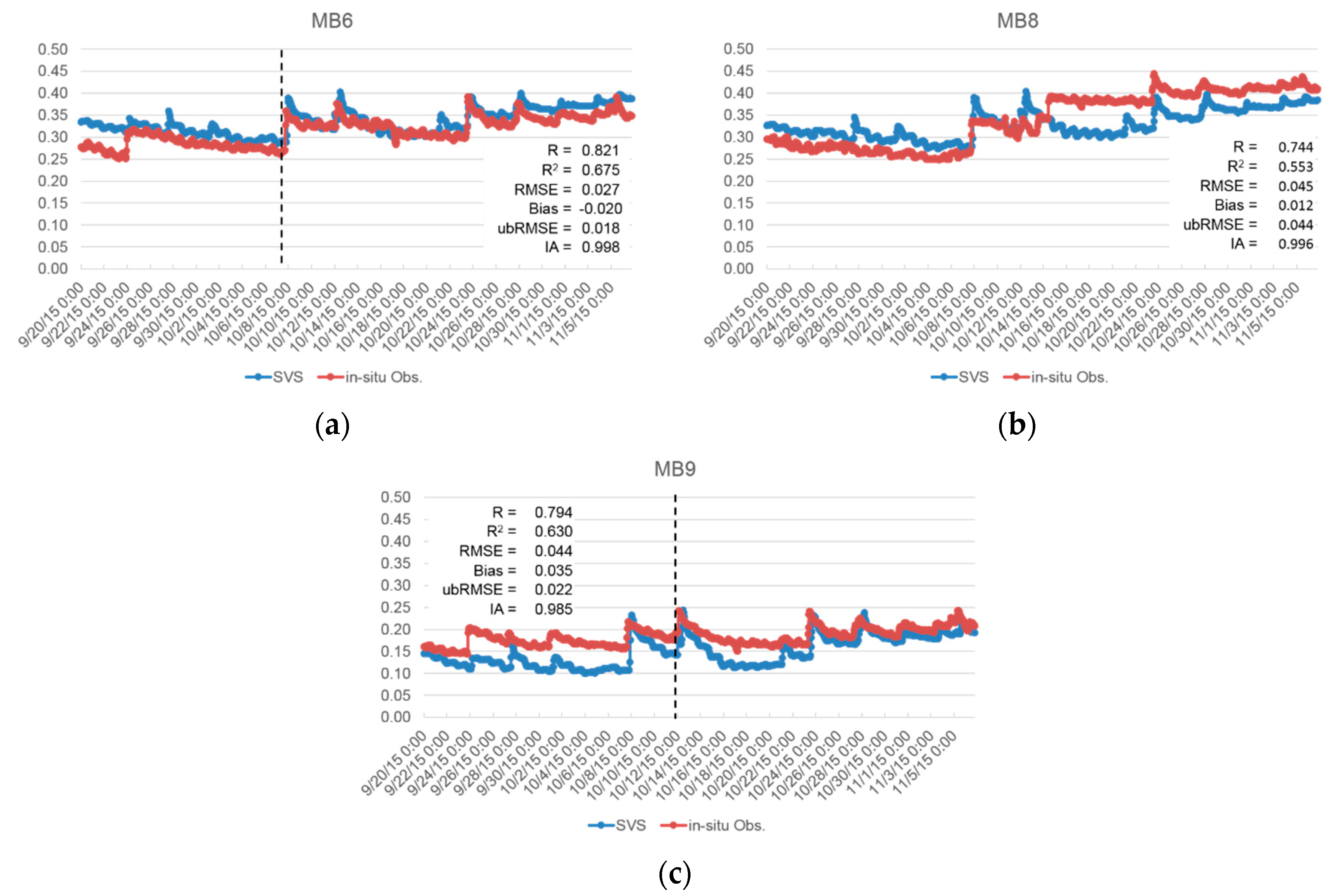
4.1. Verification against In Situ Observations

Soil moisture observations from Real-time In-situ Soil Monitoring for Agriculture (RISMA) stations located in the east and southeast part of the experimental site were available (Figure 1). Herein, the simulated soil moisture by the SVS model is compared with respect to the observed evolution of soil moisture as recorded by the stations during the study period (20 September 2015 to 6 November 2015). Herein, the correlation (R), goodness of fit (R2), Root Mean Square Error (RMSE), mean bias, unbiased RMSE (ubRMSE) [35,36] and the Index of Agreement (IA) [14] are used as statistical indices for the verification of the SVS model performance over the experimental site. Since the performance of the SVS model in soil moisture simulation has extensively been verified against in situ observations in [15,17,25,26], we indicatively selected three out of the six RISMA stations to additionally verify the performance of the SVS model in our experimental site. The selected stations are the MB6, MB8 and MB9 (Figure 1). The MB6 and MB8 stations are located over clay, while the MB9 station is located over sand. The MB6 and MB8 stations were selected intentionally because the highest and lowest performance of the SVS model was obtained over these stations, respectively. Figure 6 shows the soil moisture evolution in time as simulated by the SVS model and observed by the three RISMA stations. Soil moisture observation from the RISMA stations is vertically measured for the top 5 cm soil layer. As shown in Figure 6, soil moisture simulation results from the SVS model exhibit high R with the in situ observations, varying between 0.744 (MB8) to 0.821 (MB6). The lowest RMSE and ubRMSE are obtained in the MB6 station (0.027 m3m−3 and 0.018 m3m−3, respectively) and reach the maximum of 0.045 m3m−3 and 0.044 m3m−3, respectively, in the MB8 station. Small bias values are shown in the three RISMA stations with the highest to be equal to 0.022 m3m−3 in the MB9 station. The IA is >0.9 in all three stations. These results confirm the high performance of the SVS model in simulating the time evolution of the surface soil moisture.
The soil moisture retrievals from SAR imagery are also verified against the in situ observations recorded at the six RISMA stations. Table 2 presents the observed and retrieved soil moisture.
Observed soil moisture values in Table 2 on each date correspond to the average recorded soil moisture values in the locations of the RISMA stations at the time of ascending and descending passes of the satellite. Table 2 also presents the mean difference between the observed and retrieved soil moisture for each date. As shown in Table 2, the mean difference between the observed and retrieved soil moisture using SAR imagery varies between 0.013 m3m−3 on 2 November to 0.067 m3m−3 on 19 October. The overall mean difference between the observed and retrieved soil moisture over the four dates is equal to 0.047 m3m−3. This value agrees with the obtained mean absolute error (0.04 m3m−3) reported in an extensive verification study of the soil moisture retrieval algorithm presented in [14].

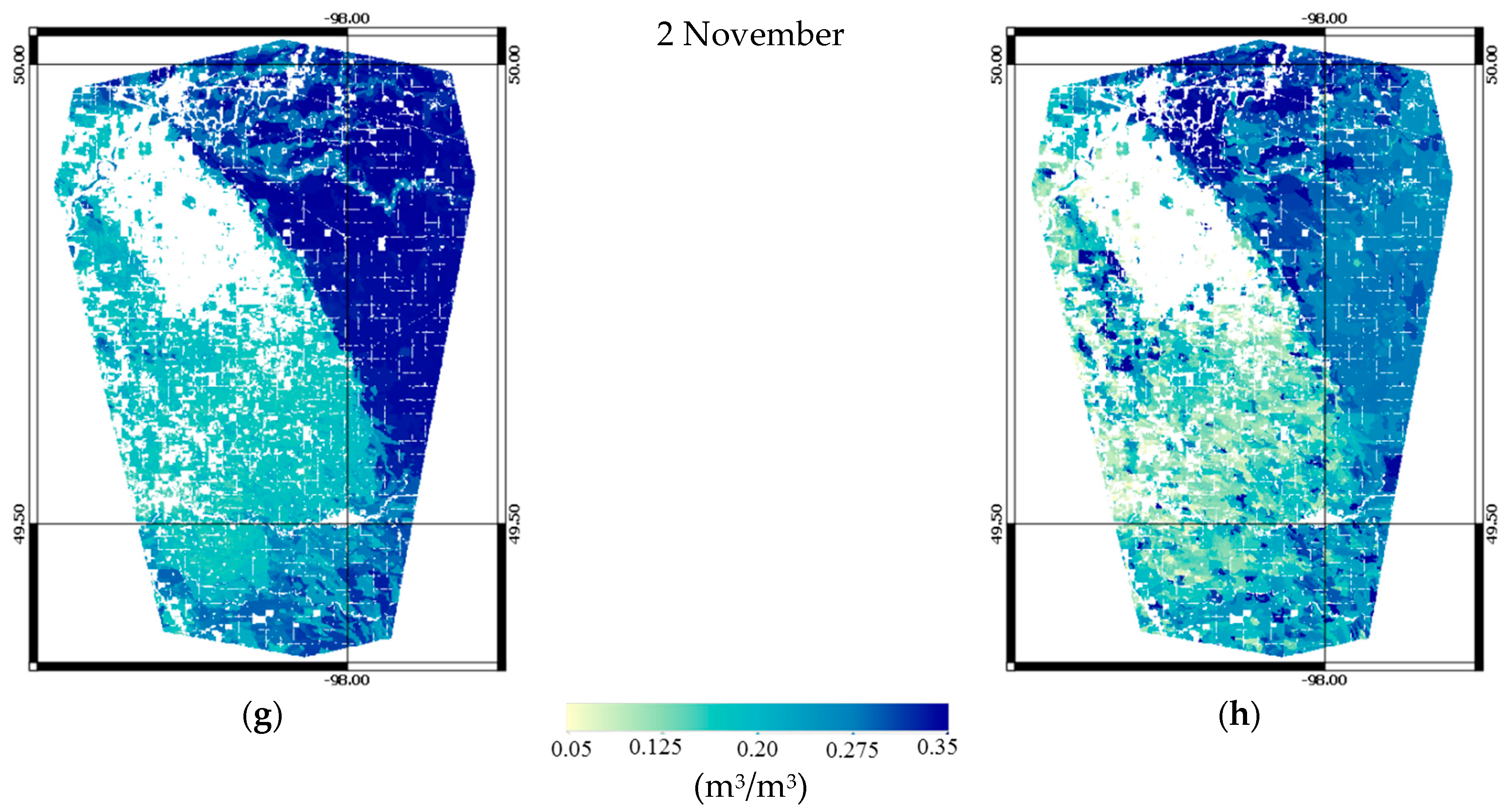
4.2. Qualitative Analysis

For the evaluation of soil moisture to be of similar spatial and temporal scale: (1) we average the SAR soil moisture maps obtained by the AAFC retrieval algorithm and the SVS simulated soil moisture using the soil texture polygons (Figure 3), hence one soil moisture value is obtained within each polygon, and (2) we compare the resulting SAR soil moisture maps averaged by the soil texture polygons with the average of the two SVS soil moisture maps simulated at the ascending and descending times of the satellite pass. Figure 7 shows the SVS simulated soil moisture and the estimated soil moisture using SAR imagery for the aforementioned four dates, after the averaging. In Figure 7, gaps (white) indicate regions excluded from our study, such as wetlands, roads, and the forest area in the northwestern part of the experimental site.
Blue areas in Figure 7 indicate soils with higher moisture content, while red areas indicate drier soils. As shown in Figure 7, detailed spatial variations of soil moisture are captured using the SVS model (Figure 7a,c,e,g), which in many cases qualitatively match the spatial variations of the SAR-derived soil moisture (Figure 7b,d,f,h). However, we note that the retrieved soil moisture maps from the SAR data still show some small-scale soil moisture variations not captured in the SVS model output. This is likely due to the higher spatial resolution associated with the SAR images (Table 1). Figure 7 shows the capability of the SVS model to differentiate the drier soils associated with sandier textures (central and western areas) from wetter clay soils (eastern and northeastern areas).
Qualitatively, the simulated soil moisture using the SVS model on 25 September (Figure 7a) is fairly comparable to the SAR estimated soil moisture (Figure 7b). The archived weather information showed that a significant precipitation event took place on 23 September and reached the 10.6 mm. Temperatures were high and reached daily maximum of 21.3 °C on 23 September and 19.5 °C on 24 September. Thus, the comparable results on 25 September indicate that soil layers sensed by SAR and by the SVS were relatively dry with fairly similar soil moisture contents. The SVS model tends to considerably overestimate the soil moisture, especially over clay (east and northeast of the experimental site) on 9 October (Figure 7c) in comparison to the SAR product (Figure 7d). This overestimation could be an effect of the sensing depth of the two soil moisture approaches, where in the case of SVS the soil moisture simulation is for the top soil layer with depth of 5 cm, while in the case of SAR the soil moisture is estimated for the top soil surface with a sensing depth which should be less than 5 cm for C-band SAR, depending on the soil type and moisture content [37,38]. We examined the archived weather information for the experimental site and noted that on 7 October (two days before SAR imagery acquisition) a significant precipitation event took place in the area with accumulation as high as 11.8 mm. The air temperature on 7 and 8 October was moderate and reached a maximum of 12.1 °C on 7 October. Thus, it appears that the overestimation of soil moisture by the SVS, in comparison to SAR output, on 9 October might be the results of the top soil layer sensed by SAR (<5 cm) drying faster than the top 5 cm soil simulated by the SVS model. This is also confirmed in Figure 6a, where we note that following the precipitation event on 7 October (dashed vertical line) the simulated SVS soil moisture values between 7 October and 9 October are very close to the observed soil moisture values recorded at the MB6 RISMA station for the top 5 cm soil layer. It is worth mentioning that the MB6 RISMA station is located over clay soil.
On 19 October, SVS appears to generally underestimate soil moisture (Figure 7e) in comparison to the SAR product (Figure 7f). Looking at the archived weather information, we found that the experimental site had no precipitation between 13 and 19 October, with the last precipitation event being on 12 October. Also, the air temperature at that period was relatively high and reached a maximum of 20.1 °C on 18 October. Based on this weather information, one would expect the SVS and SAR-based soil moisture results in Figure 7e and 7f, respectively, to be comparable since both the top soil layers sensed by SAR and the top 5 cm sensed by the SVS model should be dry. Thus, the underestimation of the soil moisture provided by the SVS model suggests bias which could be related to the SVS physical model, possibly its representation of evaporation over bare soil. This tendency of the SVS to dry down quickly following a precipitation event (in our case it was on 12 October) has been previously observed in [25]. Looking at Figure 7e,f, it appears that this bias is higher over lighter sandier soils (center and western areas). This tendency of the SVS to dry down quickly following a precipitation event is confirmed in Figure 6c, where it is shown that following the precipitation event on 12 October (dashed vertical line) the SVS underestimated the soil moisture compared to the in situ observations. It is worth mentioning that the MB9 RISMA station (Figure 6c) is located in lighter sandier soil. This tendency of the SVS to dry down quickly following a precipitation event was not observed in the SVS results of 9 October because the time difference between the precipitation event and the simulated SVS soil moisture was very small (less than two days). Thus, time was not enough for the SVS model bias to be observed.
Figure 7g shows that the simulated soil moisture is fairly comparable to the estimated soil moisture using SAR (Figure 7h) on 2 November. Archived weather information showed that on 31 October a precipitation event took place in the area with accumulation of 4.2 mm. Also, on 1 November, a weak precipitation event occurred with accumulation of 0.6 mm. Temperatures were also moderate and reached a maximum of 9.6 °C and 9.8 °C on 31 October and 1 November, respectively. The comparable results of 2 November indicate that both the soil moisture layers sensed by SAR and SVS were wet, especially over clay.
Visually, the highest overall deviation between the simulated soil moisture from SVS and the estimated soil moisture using the SAR imagery is on 9 October, where SVS (Figure 7c) appears to overestimate the soil moisture values in comparison to SAR (Figure 7d). The highest overall agreement between the two soil moisture products (SVS and SAR) is visually observed on 25 September. It is worth mentioning that antecedent soil moisture conditions are a factor contributing to the observed differences between SVS and SAR soil moisture results. However, we focused our analysis of results on the air temperature and precipitation, since these are the most important atmospheric inputs controlling soil moisture, especially in the superficial or surface layer.

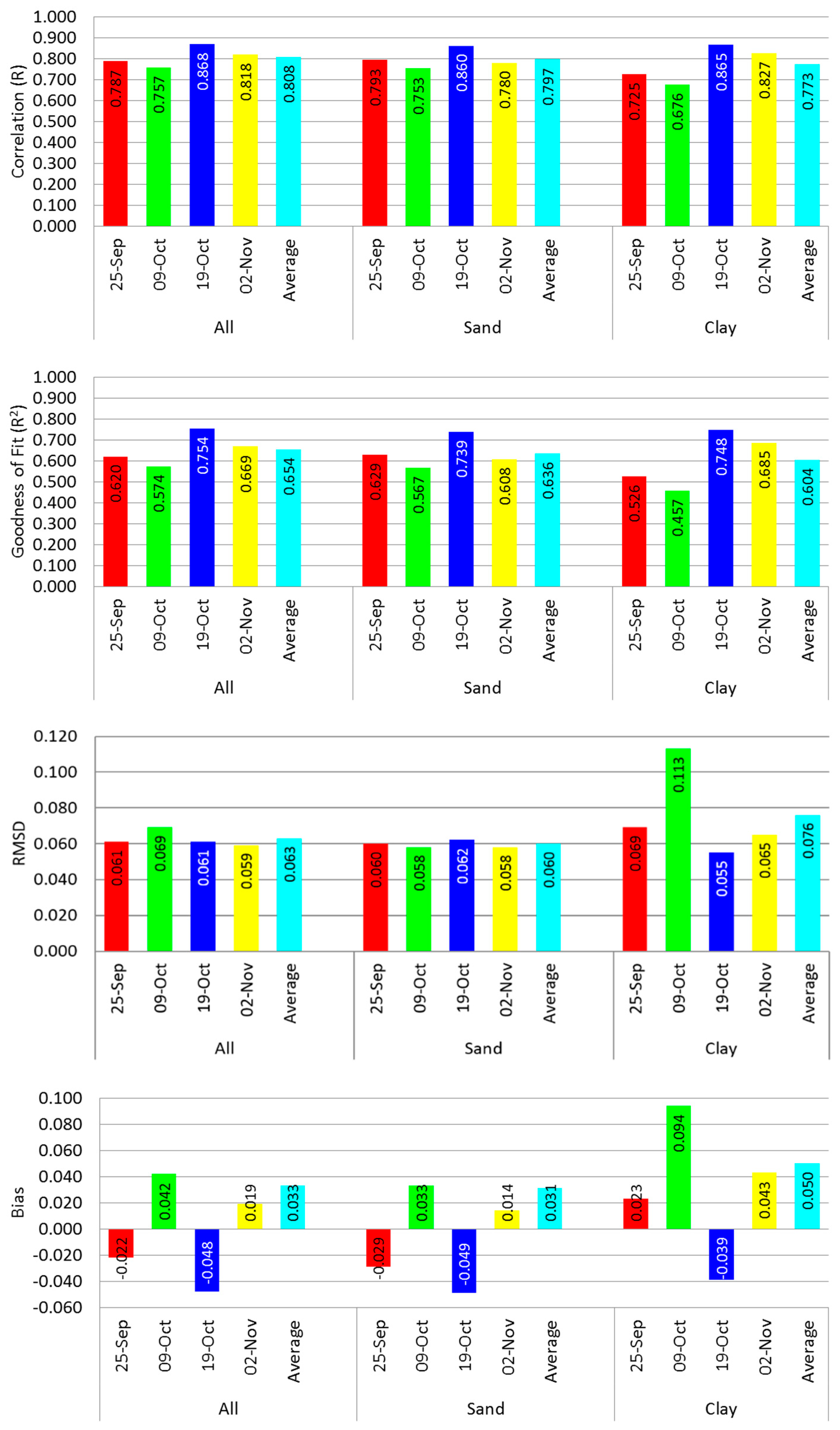
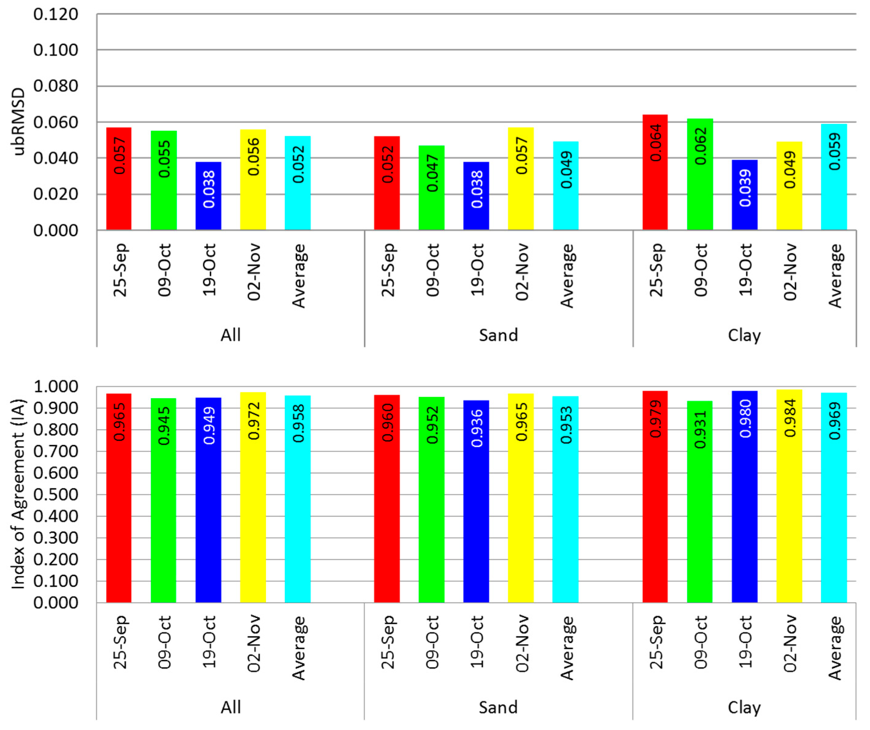
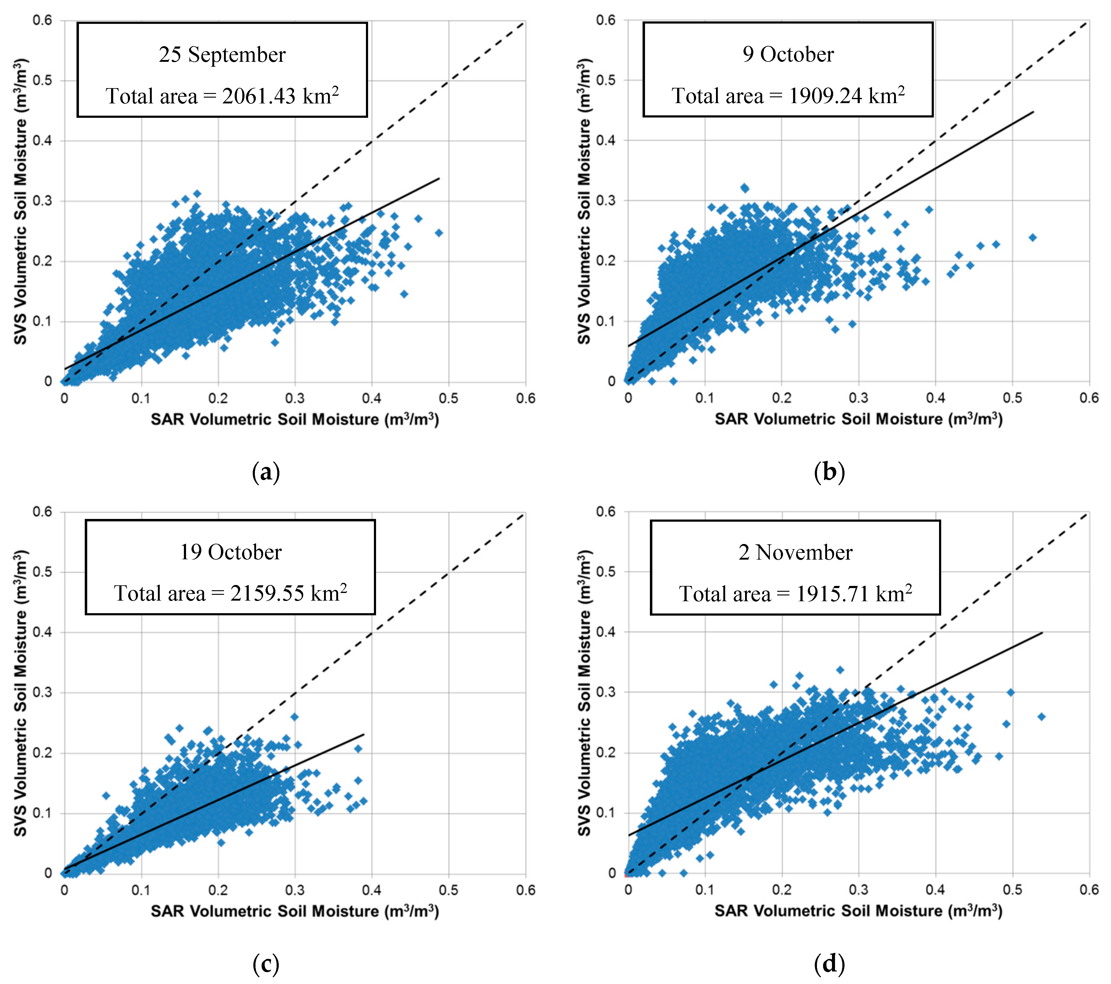
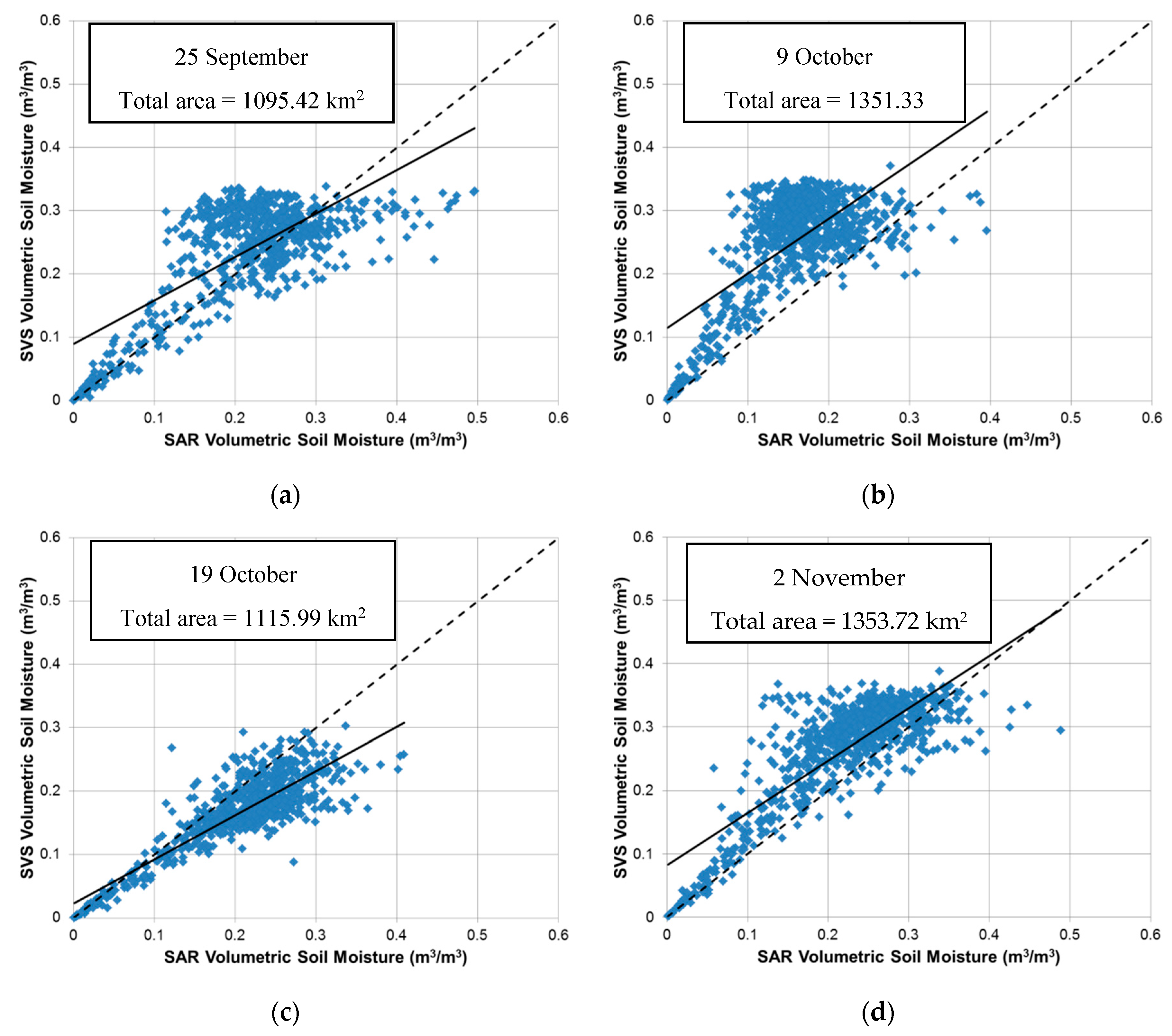
4.3. Quantitative Analysis

A statistical evaluation of the SVS soil moisture results was conducted against the estimated soil moisture content from SAR imagery. The six aforementioned statistical indices were used to quantitatively validate the SVS simulated soil moisture against the SAR estimated soil moisture (Figure 8). Herein, we referred to the RMSE as Root Mean Square Difference (RMSD) to emphasize that both SAR soil moisture retrievals and SVS soil moisture simulations contain errors. In addition to the statistical validation indices, we further investigated the results of the SVS model by creating scatterplots which compare the SVS simulated soil moisture with the estimated soil moisture using SAR imagery. One can see in Figure 9 that the disagreement in the soil moisture between SVS and SAR-based approaches increases as soil moisture increases, especially for higher volumetric soil moisture (>0.35 m3m−3). From the four scatterplots in Figure 9, the SVS model appears to have a peak of soil moisture values ~0.35 m3m−3. As evident in Figure 9c, the SVS model underestimated soil moisture on 19 October. This underestimation is reflected in Figure 8, where the largest absolute mean bias (0.048 m3m−3) is reported for the results associated with this date. The negative mean bias on 19 October indicates that the underestimation of the SVS model resulted in drier soils compared to the estimated soil moisture from SAR. This agrees with our visual interpretation of the SVS results in Figure 7e against the SAR-based results in Figure 7f. The absolute mean bias of 19 October (0.048 m3m−3) is slightly larger than that of 9 October (0.042 m3m−3), which visually (Figure 7c) appeared to have the highest overall deviation from the SAR-based soil moisture product (Figure 7d). Note that the positive mean bias associated with the 9 October results indicates that the soil is modeled to be wetter relative to the SAR-based estimates. The lowest absolute mean bias (0.019 m3m−3) is given by the SVS results of 2 November, as presented in Figure 8.
As provided in Figure 8, while the soil moisture results of 19 October have the largest absolute mean bias (0.048 m3m−3), the simulated soil moisture values have the highest correlation and goodness of fit values (0.868 and 0.754, respectively) with the estimated soil moisture. This is reflected in Figure 9c which shows a tighter distribution of data points with fewer outliers. Removing the bias from the 19 October results achieves the lowest discrepancy between the SVS and SAR results (ubRMSD = 0.038 m3m−3). We note in Figure 8 that the soil moisture results of 9 October give the lowest cross correlation and goodness of fit (0.757 and 0.574, respectively) values. Also, the results on this date have the lowest index of agreement (0.945) and the largest RMSD (0.069 m3m−3), which is reduced to 0.055 m3m−3 after bias removal. This reduced performance agrees with our previous visual comparison between the SVS model (Figure 7c) and SAR imagery results (Figure 7d). The highest index of agreement is achieved for the 2 November output (0.972), which explains the lowest absolute mean bias values (0.019 m3m−3) of all the soil moisture results. These results indicate varying, but good overall performance of the SVS land surface model in soil moisture simulation. We note from Figure 8 that the correlations between the soil moisture simulated using SVS and estimated using SAR are higher than those reported between the simulated and measured soil moisture in [13]. This could be related to the fact that the SVS model was evaluated in [13] during the summer, where crops in the experimental site affect the soil moisture simulation results, while in our case the evaluation of the SVS model is conducted during the fall season over bare soil or sparsely-vegetated areas. Also, in [1], evaluation was conducted against fewer point observations, which should be representatively and statistically less stable compared to our study.

4.4. Soil Moisture as a Function of the Soil Texture

4.4.1. Sand

SVS soil moisture results (Figure 7) are divided based on soil texture into two groups; soils dominated by coarser textured sediments (sands) and finer textured clay (Figure 3). This was achieved by dividing the soil polygons into sand and clay polygons based on the sand and clay fractions within these polygons. Polygons where the fraction of clay in the soils is greater than 40% are categorized as clay polygons, while polygons with clay fractions less than 40% are categorized as sand. The 40% threshold value is defined based on the soil texture triangle [39]. The threshold value of 40% is a reasonable value that was successfully proposed in [40] to define soil with predominance of clay. Although the 40% threshold ensures the dominance of clay in the clay polygons, it does not exclude the possible presence of loam in the sand polygons. The total area in square kilometers of polygons corresponding to sand and clay are reported in Figure 9 and Figure 10, respectively, for each date. Based on the calculated total area of polygons, we find that approximately 60–65% of the experimental site is sand and the rest is clay.
The same process was also applied to the estimated soil moisture using the SAR imagery (Figure 7), leading to texture-based comparisons between the SVS modeled and SAR estimated soil moisture. Scatterplots which compare the simulated soil moisture using the SVS model with the estimated soil moisture using SAR imagery over the sand polygons are shown in Figure 10. In addition, the previous statistical evaluation of soil moisture was reapplied by recalculating the six validation indices over sand (Figure 8). As shown in Figure 10, scatterplots over sand dominated soils are similar to the scatterplots presented in Figure 9 for all polygons regardless of the soil texture. Again, the results of the SVS model on 19 October (Figure 10c) have the highest cross correlation (0.860) and goodness of fit (0.739) in comparison to the estimated soil moisture (Figure 8), yet this date has the highest absolute mean bias (0.049 m3m−3) with underestimation (negative mean bias) of soil moisture by the SVS model (Figure 10c). This underestimation was clearly visible over the drier soil in the center and western areas in Figure 7e. Removing this bias reduces the RMSD from 0.062 m3m−3 on 19 October (highest among the four dates) to 0.038 m3m−3 (lowest ubRMSD). On the other hand, the simulated soil moisture by the SVS model on 9 October has the lowest cross correlation (0.753) and the lowest goodness of fit (0.567) values when compared against the moisture estimated using SAR (Figure 8). We note that Figure 8 shows a relatively consistent RMSD over sand with minor differences in the RMSD values among the four dates. Yet when the bias is removed, differences in the ubRMSD statistics among the four dates are notable. The absolute mean bias is the lowest on 2 November (0.014 m3m−3). This is reflected in the index of agreement value between the SVS and SAR outputs, which was highest on 2 November (0.965). However, removing this bias from the RMSD (0.058 m3m−3) leads to an ubRMSD of 0.057 m3m−3, which is the highest ubRMSD for sand.

4.4.2. Clay

Scatterplots corresponding to the soil moisture over clay are shown in Figure 11. The six statistical validation indices were recalculated for the evaluation of the SVS model performance over clay dominated soils (Figure 8). Similar to the results from the sandier soils, the highest correlation (0.865) and goodness of fit (0.748) between the simulated and estimated soil moisture is for 19 October. In this case, fewer outliers are observed (Figure 11c). The overestimation of the soil moisture by the SVS model is clearly visible in Figure 11b and reflected by the statistical validation indices in Figure 8, where the results of 9 October show the lowest correlation (0.676), goodness of fit (0.457) and index of agreement (0.931) and the largest RMSD (0.113 m3m−3) and absolute mean bias (0.094 m3m−3) among the four dates. This overestimation (positive mean bias) of soil moisture by the SVS model agrees with the previous visual interpretation of the results (Figure 7c). With the exception of 9 October results, we note that in terms of RMSD the SVS model performs better over sand compared to clay (Figure 8). Once the bias is removed, the SVS model has even better agreement with the SAR-based estimates over sandier textured soils, with the exception of 2 November (0.057 m3m−3 on sand and 0.049 m3m−3 on clay). The index of agreement between the modeled soil moisture and the SAR-based estimated soil moisture is high over both sand and clay (IA > 0.9), with clay dominated polygons in slightly better agreement, except for 9 October (Figure 8). Comparing the average values of the statistic indices in Figure 8, it can be noted that the SVS model performs better over sand than clay with the exception of the index of agreement. As for the sand, the lowest ubRMSD for clay is observed on 19 October.

4.5. Limitations

A limitation of our study is the restriction of the study period between late September (after the growing season) and early November (before the onset of snow). Thus, additional comparison studies should be conducted during, e.g., the vegetation growth period in the summer. However, in this case L-band SAR data with higher penetration capabilities would be necessary in order to retrieve the soil moisture under the vegetation canopy. Another limitation of our study is the limited number of days in which the comparison is performed. This is due to the fact that the RADARSAT-2 satellite does not have a standard coverage acquisition plan. This limitation is expected to be resolved with the launch of the Canadian RADARSAT Constellation Mission (RCM) in 2019. The RCM will be a constellation of three SAR satellites which are expected to provide daily complete coverage of Canada’s territory and marine regions. Although the SVS model performance in soil moisture simulation has been verified against in situ observations in [15,17,25,26], additional verification of the SVS soil moisture simulations and the SAR soil moisture retrievals in the selected experimental site would have been useful. However, that would require large number of in situ soil moisture observations homogeneously collected over our large selected experimental site, which might not be easily feasible.

5. Conclusions

Soil moisture values simulated at the field scale by the Soil, Vegetation, and Snow (SVS) land surface model developed at Environment and Climate Change Canada (ECCC) were compared against soil moisture values estimated using Synthetic Aperture Radar (SAR) imagery. Surface soil moisture was estimated from RADARSAT-2 satellite data using a physical scattering model and pairs of ascending and descending image acquisitions. Averaged over homogeneous soil texture polygons, soil moisture maps generated from SAR imagery and simulated using the SVS model were compared. This was the first attempt to evaluate the high resolution (sub-km) soil moisture output of the SVS model against soil moisture estimated over a large geospatial extent. The soil moisture values simulated by the SVS model showed an overall good correlation (consistently >0.70 except for 9 October which was slightly lower than 0.70) and therefore goodness of fit with those estimated using SAR imagery. This is further confirmed with the index of agreement which was consistently above 0.90. The RMSD values were below 0.10 m3m−3, with the exception on 9 October over clay (0.11 m3m−3). The overestimation or underestimation of the soil moisture by the SVS model tends to be more apparent over clay rather than sand. This is confirmed by the absolute mean bias values which are always higher over clay in comparison to sand, with the exception of the results on 25 September, where the absolute mean bias was slightly higher over sand. Although the overall performance of the SVS land surface model is good, the problem with dry-downs which are too rapid in the SVS was noted. This was evident in the underestimation of soil moisture for the SVS results of 19 October. This is a model deficiency which we are currently addressing by modifying the formulation of dry soil evaporation. Future work would explore the potential of assimilation of both retrieved soil moisture from SAR imagery and SAR backscatter using a forward model in the Canadian Land Data Assimilation System (CaLDAS).

Author Contributions

L.S. and M.L.C. simulated the soil moisture using the SVS model and M.F. estimated the soil moisture from the SAR imagery. M.D. conducted the statistical analysis of the results. All authors contributed to the writing of the paper.

Funding

Research funding was provided by the Canadian Space Agency under the Data Utilization Application Plan (DUAP) of the RADARSAT Constellation Mission (RCM).

Acknowledgments

RADARSAT-2 data and products © MacDonald, Dettwiler and Associates Ltd. (2013)—All Rights Reserved. RADARSAT is an official mark of the Canadian Space Agency.

Conflicts of Interest

The authors declare no conflict of interest.

References

  1. National Research Council. Issues in the Integration of Research and Operational Satellite Systems for Climate Research: Part I Science and Design; The National Academies Press: Washington, DC, USA, 2000. [Google Scholar]
  2. Eltahir, E.A.B. A soil moisture-rainfall feedback mechanism, 1. Theory and observations. Water Resour. Res. 1998, 34, 765–776. [Google Scholar] [CrossRef]
  3. Findell, K.L.; Eltahir, E.A.B. Atmospheric controls on soil moisture-boundary layer interactions. Part 1: Framework development. J. Hydrometeorol. 2003, 4, 552–569. [Google Scholar] [CrossRef]
  4. Trier, S.; Chen, F.; Manning, K.W.; LeMone, M.A.; Davis, C.A. Sensitivity of the PBL and precipitation in 12-day simulations of warm-season convection using different land surface models and soil wetness conditions. Mon. Weather Rev. 2008, 136, 2321–2343. [Google Scholar] [CrossRef]
  5. Seneviratne, S.I.; Corti, T.; Davin, E.L.; Hirschi, M.; Jaeger, E.B.; Lehner, I.; Orlowsky, B.; Teuling, A.J. Investigating soil moisture-climate interactions in a changing climate: A review. Earth-Sci. Rev. 2010, 99, 126–161. [Google Scholar] [CrossRef]
  6. Evans, C.; Schumacher, R.S.; Galarneau, T.J., Jr. Sensitivity in the overland reintensification of tropical cyclone Erin (2007) to near-surface soil moisture characteristics. Mon. Weather Rev. 2011, 139, 3848–3870. [Google Scholar] [CrossRef]
  7. Pablos, M.; Martínez-Fernández, J.; Piles, M.; Sánchez, N.; Vall-llossera, M.; Camps, A. Multi-temporal evaluation of soil moisture and land surface temperature dynamics using in Situ and Satellite Observations. Remote Sens. 2016, 8, 587. [Google Scholar] [CrossRef]
  8. Bolten, J.D.; Crow, W.T.; Zhan, X.; Jackson, T.J.; Reynolds, C.A. Evaluating the utility of remotely sensed soil moisture retrievals on operational agricultural drought monitoring. IEEE J. Sel. Top. Appl. Earth Obs. Remote Sens. 2010, 3, 57–66. [Google Scholar] [CrossRef]
  9. Champagne, C.; Davidson, A.; Cherneski, P.; L’Heureux, J.; Hadwen, T. Monitoring agricultural risk in Canada using L-band passive microwave soil moisture from SMOS. J. Hydrometeorol. 2015, 16, 5–18. [Google Scholar] [CrossRef]
  10. Champagne, C.; Rowlandson, T.; Berg, A.; Burns, T.; L’Heureux, J.; Tetlock, E.; Adams, J.; McNairn, H.; Toth, B.; Itensifu, D. Satellite surface soil moisture from SMOS and Aquarius: Assessment for applications in agricultural landscapes. Int. J. Appl. Earth Obs. Geoinf. 2016, 45, 143–154. [Google Scholar] [CrossRef]
  11. Lievens, H.; Tomer, S.K.; Al Bitar, A.; De Lannoy, G.J.M.; Drusch, M.; Dumedah, G.; Hendricks Franssen, H.-J.; Kerr, Y.H.; Martens, B.; Pan, M.; et al. SMOS soil moisture assimilation for improved hydrologic simulation in the Murray Darling Basin, Australia. Remote Sens. Environ. 2015, 168, 146–162. [Google Scholar] [CrossRef]
  12. Crow, W.T.; Chen, F.; Reichle, R.H.; Liu, Q. L band microwave remote sensing and land data assimilation improve the representation of prestorm soil moisture conditions for hydrologic forecasting. Geophys. Res. Lett. 2017, 44, 5495–5503. [Google Scholar] [CrossRef] [PubMed]
  13. Garnaud, C.; Bélair, S.; Carrera, M.; McNairn, H.; Pacheco, A. Field-scale spatial variability of soil moisture and L-Band Brightness Temperature from Land Surface Modeling. J. Hydrometeorol. 2017, 18, 573–589. [Google Scholar] [CrossRef]
  14. Merzouki, M.; McNairn, H. A hybrid (multi-angle and multipolarization) approach to soil moisture retrieval using the integral equation model: Preparing for the RADARSAT constellation mission. Can. J. Remote Sens. 2015, 41, 349–362. [Google Scholar] [CrossRef]
  15. Alavi, N.; Bélair, S.; Fortin, V.; Zhang, S.; Husain, S.Z.; Carrera, M.L.; Abrahamowicz, M. Warm season evaluation of soil moisture prediction in the Soil, Vegetation, and Snow (SVS) scheme. J. Hydrometeorol. 2016, 17, 2315–2332. [Google Scholar] [CrossRef]
  16. Koster, R.D.; Suarez, M.J.; Ducharne, A.; Stieglitz, M.; Kumar, P. A catchment-based approach to modeling land surface processes in a general circulation model: 1. Model structure. J. Geophys. Res. 2000, 105, 24809–24822. [Google Scholar] [CrossRef]
  17. Carrera, M.; Bélair, S.; Bilodeau, B. The Canadian land data assimilation system (CaLDAS): Description and synthetic evaluation study. J. Hydrometeorol. 2015, 16, 1293–1314. [Google Scholar] [CrossRef]
  18. Milbrandt, J.A.; Bélair, S.; Faucher, M.; Vallée, M.; Carrera, M.L.; Glazer, A. The Pan-Canadian High-Resolution (2.5 km) Deterministic Prediction System. Weather Forecast. 2016, 31, 1791–1816. [Google Scholar] [CrossRef]
  19. Noilhan, J.; Planton, S. A simple parameterization of land surface processes for meteorological models. Mon. Weather Rev. 1989, 117, 536–549. [Google Scholar] [CrossRef]
  20. Noilhan, J.; Mahfouf, J.-F. The ISBA land surface parameterization scheme. Glob. Planet. Chang. 1996, 13, 145–159. [Google Scholar] [CrossRef]
  21. Bélair, S.; Crevier, L.-P.; Mailhot, J.; Bilodeau, B.; Delage, Y. Operational implementation of the ISBA land surface scheme in the Canadian regional weather forecast model. Part I: Warm season results. J. Hydrometeorol. 2003, 4, 352–370. [Google Scholar] [CrossRef]
  22. Bélair, S.; Brown, R.; Mailhot, J.; Bilodeau, B.; Crevier, L.-P. Operational implementation of the ISBA land surface scheme in the Canadian regional weather forecast model. Part II: Cold season results. J. Hydrometeorol. 2003, 4, 371–386. [Google Scholar] [CrossRef]
  23. Husain, S.Z.; Alavi, N.; Bélair, S.; Carrera, M.; Zhang, S.; Fortin, V.; Abrahamowicz, M.; Gauthier, N. The multibudget soil, vegetation, and snow (SVS) scheme for land surface parameterization: Offline warm season evaluation. J. Hydrometeorol. 2016, 17, 2293–2313. [Google Scholar] [CrossRef]
  24. Soulis, E.D.; Snelgrove, K.R.; Kouwen, N.; Seglenieks, F.; Verseghy, D.L. Towards closing the vertical water balance in Canadian atmospheric models: Coupling of the land surface scheme class with the distributed hydrological model watflood. Atmos. Ocean 2000, 38, 251–269. [Google Scholar] [CrossRef]
  25. Garnaud, C.; Bélair, S.; Berg, A.; Rowlandson, T. Hyperresolution Land Surface Modeling in the Context of SMAP Cal–Val. J. Hydrometeorol. 2016, 17, 345–352. [Google Scholar] [CrossRef]
  26. Maheu, A.; Anctil, F.; Gaborit, É.; Fortin, V.; Nadeau, D.; Therrien, R. A field evaluation of soil moisture modelling with the Soil, Vegetation, and Snow (SVS) land surface model using evapotranspiration observations as forcing data. J. Hydrol. 2018, 558, 532–545. [Google Scholar] [CrossRef]
  27. Rüdiger, C.; Calvet, J.; Gruhier, C.; Holmes, T.R.; de Jeu, R.A.; Wagner, W. An intercomparison of ERS-Scat and AMSR-E soil moisture observations with model simulations over France. J. Hydrometeorol. 2009, 10, 431–447. [Google Scholar] [CrossRef]
  28. Al-Yaari, A.; Wigneron, J.P.; Ducharne, A.; Kerr, Y.; de Rosnay, P.; de Jeu, R.; Govind, A.; Al Bitar, A.; Albergel, C.; Muñoz-Sabater, J.; et al. Global-scale evaluation of two satellite-based passive microwave soil moisture datasets (SMOS and AMSR-E) with respect to Land Data Assimilation System estimates. Remote Sens. Environ. 2014, 149, 181–195. [Google Scholar] [CrossRef]
  29. McNairn, H.; Jackson, T.J.; Wiseman, G.; Belair, S.; Berg, A.; Bullock, A.; Colliander, A.; Cosh, M.H.; Kim, S.-B.; Magagi, R.; et al. The soil moisture active passive validation experiment 2012 (SMAPVEX12): Prelaunch Calibration and Validation of the SMAP Soil Moisture Algorithms. IEEE Trans. Geosci. Remote Sens. 2015, 53, 2784–2801. [Google Scholar] [CrossRef]
  30. Michalyna, W.; Podolsky, G.; Jacques, S. Soils of the Rural Municipalities of Grey, Dufferin, Roland, Thompson and Part of Stanley; Report D60; Agriculture and Agri-Food Canada, Manitoba Agriculture and the University of Manitoba: Winnipeg, MB, Canada, 1988. [Google Scholar]
  31. Bhumralkar, C.M. Numerical experiments on the computation of ground surface temperature in an atmospheric general circulation model. J. Appl. Meteorol. 1975, 14, 1246–1258. [Google Scholar] [CrossRef]
  32. Mahfouf, J.-F.; Brasnett, B.; Gagnon, S. A Canadian Precipitation Analysis (CaPA) project: Description and preliminary results. Atmos. Ocean 2007, 45, 1–17. [Google Scholar] [CrossRef]
  33. Fung, A.K.; Li, Z.; Chen, K.S. Backscattering from a randomly rough dielectric surface. IEEE Trans. Geosci. Remote Sens. 1992, 30, 356–369. [Google Scholar] [CrossRef]
  34. Hallikainen, M.T.; Ulaby, F.T.; Dobson, M.C.; El-rayes, M.A.; Wu, L. Microwave dielectric behavior of wet soil-part 1: Empirical models and experimental observations. IEEE Trans. Geosci. Remote Sens. 1985, 23, 25–34. [Google Scholar] [CrossRef]
  35. Entekhabi, D.; Reichle, R.H.; Koster, R.D.; Crow, W.T. Performance metrics for soil moisture retrievals and application requirements. J. Hydrometeorol. 2010, 11, 832–840. [Google Scholar] [CrossRef]
  36. Zhang, X.; Zhang, T.; Zhou, P.; Shao, Y.; Gao, S. Validation analysis of SMAP and AMSR2 soil moisture products over the United States using ground-based measurements. Remote Sens. 2017, 9, 104. [Google Scholar] [CrossRef]
  37. Ulaby, F.T.; Moore, R.K.; Fung, A.K. Microwave Remote Sensing: Active and Passive—Volume 2: Radar Remote Sensing and Surface Scattering and Emission Theory; Artech House: Norwood, MA, USA, 1982. [Google Scholar]
  38. Koyama, C.N.; Liu, H.; Takahashi, K.; Shimada, M.; Watanabe, M.; Khuut, T.; Sato, M. In-Situ Measurement of Soil Permittivity at Various Depths for the Calibration and Validation of Low-Frequency SAR Soil Moisture Models by Using GPR. Remote Sens. 2017, 9, 580. [Google Scholar] [CrossRef]
  39. Phogat, V.K.; Tomar, V.S.; Dahiya, R. Soil physical properties. In Soil Science: An Introduction; Rattan, R.K., Katyal, J.C., Dwivedi, B.S., Sarkar, A.K., Bhattachatyya, T., Tarafdar, J.C., Eds.; Indian Society of Soil Science: New Delhi, India, 2015; pp. 135–171. [Google Scholar]
  40. Wood, D.; Kumar, G.V. Experimental observation of behaviour of heterogeneous soils. Mech. Cohesive-Frict. Mater. 2000, 5, 373–398. [Google Scholar] [CrossRef]
Figure 1. An aerial optical image of the location of the study area in Manitoba. The frames of each of the four dates of RADARSAT-2 SAR imagery are illustrated. Red stars indicate the locations of the Real-time In-situ Soil Monitoring for Agriculture (RISMA) stations.
Water 11 00542 g001
Figure 2. A map of the land uses in 2015 for the experimental site created by Agriculture and Agri-Food Canada (AAFC).
Water 11 00542 g002
Figure 3. Percentage of (a) sand and (b) clay in the test site.
Water 11 00542 g003
Figure 4. Representation of the hydrological process in the soil, vegetation, and snow (SVS) model.
Water 11 00542 g004
Figure 5. Flowchart of the soil moisture simulation process in using the SVS land surface model.
Water 11 00542 g005
Figure 6. Time series of hourly averaged surface soil moisture for SVS compared with observations from the (a) MB6, (b) MB8, and (c) MB9 RISMA stations. Vertical dashed lines in (a,c) indicate the simulated and observed soil moisture on 7 October and 12 October, respectively.
Water 11 00542 g006
Figure 7. Resulting averaged soil moisture maps using (a) the SVS land surface model on September 25th, (b) SAR imagery on 25 September, (c) the SVS land surface model on 9 October, (d) SAR imagery on 9 October, (e) the SVS land surface model on 19 October, (f) SAR imagery on 19 October, (g) the SVS land surface model on 2 November, and (h) SAR imagery on 2 November. Averaging was conducted based on the soil texture polygons.
Water 11 00542 g007aWater 11 00542 g007bWater 11 00542 g007c
Figure 8. Statistical validation indices for the analysis of soil moisture obtained by the SVS and the SAR imagery.
Water 11 00542 g008aWater 11 00542 g008b
Figure 9. Scatterplots of the modeled (SVS) and estimated (SAR) soil moisture for (a) 25 September, (b) 9 October, (c) 19 October, and (d) 2 November. The dashed line represents the 1:1 line and the solid line is the regression line between modeled and estimated soil moisture. Each dot represents the average soil moisture modeled (SVS) and estimated (SAR) of each soil polygon.
Water 11 00542 g009
Figure 10. Scatterplots of the modeled (SVS) and estimated (SAR) soil moisture over sand polygons for (a) 25 September, (b) 9 October, (c) 19 October, and (d) 2 November. The dashed line is the 1:1 line and solid line is the regression line. Each dot represents the average soil moisture modeled (SVS) and estimated (SAR) of each soil polygon. The total area of the sand polygons in square kilometers is indicated in each plot.
Water 11 00542 g010
Figure 11. Scatterplots of the modeled (SVS) and estimated (SAR) soil moisture over clay polygons for (a) 25 September, (b) 9 October, (c) 19 October, and (d) 2 November. The dashed line is the 1:1 line and the solid line is the regression line. Each dot represents the average soil moisture modeled (SVS) and estimated (SAR) of each soil polygon. The total area of the clay polygons in square kilometers is indicated in each plot.
Water 11 00542 g011
Table 1. A summary of the SAR imagery acquisitions. Each date consists of three image frames (Figure 1).
RADARSAT-2
Beam Mode
Acquisition
Date and Time (CDT)
Orbit DirectionIncidence AnglePixel Spacing (Range × Azimuth)
FQ8W25/09/2015
07:53:28–07:53:35
Descending27.74°4.7 m × 4.8 m
FQ10W25/09/2015
19:16:07–19:16:14
Ascending29.95°4.7 m × 5.5 m
FQ17W09/10/2015
07:45:09–07:45:17
Descending37.16°4.7 m × 5.6 m
FQ2W09/10/2015
19:07:48–19:07:53
Ascending20.74°4.7 m × 5.3 m
FQ8W19/10/2015
07:53:27–07:53:32
Descending27.73°4.7 m × 4.8 m
FQ10W19/10/2015
19:16:05–19:16:11
Ascending29.94°4.7 m × 5.5 m
FQ17W02/11/2015
07:45:08–07:45:14
Descending37.15°4.7 m × 5.6 m
FQ2W02/11/2015
19:07:46–19:07:52
Ascending20.75°4.7 m × 5.3 m
Table 2. Observed and retrieved soil moisture values at the six RISMA stations in m3m−3.
MB1MB3MB5MB6MB8MB9
Obs.SARObs.SARObs.SARObs.SARObs.SARObs.SARMean
Diff.
25 Sept.0.2060.2280.3180.3920.3490.2670.3120.1920.2750.2420.1870.1930.056
9 Oct.0.1660.1040.3060.3060.2950.2770.3240.2030.3320.2110.1930.1110.067
19 Oct.0.1720.2210.2790.2480.2950.2670.3080.3830.3820.3620.1660.0470.054
2 Nov.0.2060.1800.3220.3260.3380.3470.3430.3200.4110.3980.1970.1930.013

